long-term effects of crop-tree release on the growth and
TRANSCRIPT

University of Kentucky University of Kentucky
UKnowledge UKnowledge
Theses and Dissertations--Forestry and Natural Resources Forestry and Natural Resources
2020
Long-term Effects of Crop-tree Release on the Growth and Quality Long-term Effects of Crop-tree Release on the Growth and Quality
of Upland White Oak Stands of Upland White Oak Stands
Philip Jay Vogel University of Kentucky, [email protected] Digital Object Identifier: https://doi.org/10.13023/etd.2020.144
Right click to open a feedback form in a new tab to let us know how this document benefits you. Right click to open a feedback form in a new tab to let us know how this document benefits you.
Recommended Citation Recommended Citation Vogel, Philip Jay, "Long-term Effects of Crop-tree Release on the Growth and Quality of Upland White Oak Stands" (2020). Theses and Dissertations--Forestry and Natural Resources. 53. https://uknowledge.uky.edu/forestry_etds/53
This Master's Thesis is brought to you for free and open access by the Forestry and Natural Resources at UKnowledge. It has been accepted for inclusion in Theses and Dissertations--Forestry and Natural Resources by an authorized administrator of UKnowledge. For more information, please contact [email protected].

STUDENT AGREEMENT: STUDENT AGREEMENT:
I represent that my thesis or dissertation and abstract are my original work. Proper attribution
has been given to all outside sources. I understand that I am solely responsible for obtaining
any needed copyright permissions. I have obtained needed written permission statement(s)
from the owner(s) of each third-party copyrighted matter to be included in my work, allowing
electronic distribution (if such use is not permitted by the fair use doctrine) which will be
submitted to UKnowledge as Additional File.
I hereby grant to The University of Kentucky and its agents the irrevocable, non-exclusive, and
royalty-free license to archive and make accessible my work in whole or in part in all forms of
media, now or hereafter known. I agree that the document mentioned above may be made
available immediately for worldwide access unless an embargo applies.
I retain all other ownership rights to the copyright of my work. I also retain the right to use in
future works (such as articles or books) all or part of my work. I understand that I am free to
register the copyright to my work.
REVIEW, APPROVAL AND ACCEPTANCE REVIEW, APPROVAL AND ACCEPTANCE
The document mentioned above has been reviewed and accepted by the student’s advisor, on
behalf of the advisory committee, and by the Director of Graduate Studies (DGS), on behalf of
the program; we verify that this is the final, approved version of the student’s thesis including all
changes required by the advisory committee. The undersigned agree to abide by the statements
above.
Philip Jay Vogel, Student
Dr. John M. Lhotka, Major Professor
Dr. Steven J. Price, Director of Graduate Studies

LONG-TERM EFFECTS OF CROP-TREE RELEASE ON THE GROWTH AND QUALITY OF UPLAND WHITE OAK STANDS
THESIS
A thesis submitted in partial fulfillment of the requirements
for the degree of Master of Science in Forest and Natural Resource Sciences
By
Philip Jay Vogel
Lexington, Kentucky
Director: Dr. John M. Lhotka, Professor of Silviculture
Lexington, Kentucky
2020
Copyright© Philip Jay Vogel 2020
in the College of Agriculture, Food and Environment at the University of Kentucky

ABSTRACT OF THESIS
LONG-TERM EFFECTS OF CROP-TREE RELEASE ON THE GROWTH AND QUALITY OF UPLAND WHITE OAK STANDS
The alteration of historical disturbance regimes, forest parcelization, and varying
goals among landowners all present challenges to oak management in the eastern U.S. Foresters and landowners need tools to promote oak sustainability that are applicable on small forestland holdings and within complex management plans. From this perspective, this research evaluates a crop-tree release study installed in southeastern Kentucky in 1983. The experiment includes four, 2-acre replications of three treatment levels: 20 crop-trees per acre, 34 crop-trees per acre, and a control treatment in which crop-trees were selected but not released. Half-acre measurement plots were installed at the outset of the study. Crown class, dbh, and crop-tree grade were measured in year 0, 5, 10, 17, and 35 following treatment. Using these data, two facets of crop-tree release were analyzed: 1) how a crop-tree release affects white oak crop-trees in terms of tree growth rate and stem quality, 2) how a crop-tree release alters stand structure and per acre volume and value. Results indicate that crop-tree release applied to small sawtimber sized stands increases crop-tree diameter growth and the proportion of crop-trees reaching their maximum potential grade while promoting stand-wide growth.
KEYWORDS: Quercus alba, crop-tree release, oak silviculture, eastern U.S.
Philip Jay Vogel
May 11, 2020

LONG-TERM EFFECTS OF CROP-TREE RELEASE ON THE GROWTH AND QUALITY OF UPLAND WHITE OAK STANDS
By
Philip Jay Vogel
Dr. John M. Lhotka
Director of Thesis Dr. Steven J. Price
Director of Graduate Studies
May 8, 2020

To Olivia,
who listened to me talk
about crop-tree release
too much

iii
ACKNOWLEDGMENTS
First and foremost, I want to express my sincere gratitude to my advisor, Dr. John
Lhotka, for consistently providing thorough and helpful guidance concerning the research
presented in this work. I would also like to thank my graduate committee members, Dr.
Jeffrey Stringer, who established, preserved, and continued this study, and Dr. Thomas
Ochuodho, who helped me navigate the confusing world of economics. For funding, I
would like to recognize the University of Kentucky Department of Forestry and Natural
Resources as well as the USDA McIntire-Stennis Cooperative Forestry Research Program. I
am indebted to Zachary Hackworth, who provided counsel in the lab and assistance in the
field throughout this project, saving me countless hours of confusion. In addition, I would
like to thank Joe Frederick, Wendy Leuenberger, David Collett, and Dr. Jeffrey Stringer for
assisting in data collection.
I would also like to thank my family, who have provided love and support
throughout the years. My mother instilled in me an appreciation of nature and my father
spent many hours helping me make graphs for science fair projects. Both of these gifts have
helped me immensely over the last two years. My siblings have listened to me talk about
trees a lot, and they have even cared a little about some of it. My wife, Olivia, has shown
patience and love, and has made certain that I continue to sleep, eat, and maintain
perspective. I would also like to thank Bob Dylan for writing the lyric: “It’s not dark yet, but
it’s getting there,” which has provided me consolation throughout this endeavor. And finally,
I would like to acknowledge the Creator: “He watereth the hills from his chambers: the earth
is satisfied with the fruit of thy works.”

iv
TABLE OF CONTENTS
ACKNOWLEDGMENTS ........................................................................................................... iii
TABLE OF CONTENTS ............................................................................................................ iv
LIST OF TABLES ......................................................................................................................... vi
LIST OF FIGURES .................................................................................................................... viii
CHAPTER ONE: INTRODUCTION ........................................................................................ 1
1.1 White Oak in the Holocene Epoch ............................................................................ 1
1.2 Novel Disturbances Following European Settlement .............................................. 3
1.3 The Woods They Are A-Changin’ .............................................................................. 5
CHAPTER TWO: LITERATURE REVIEW ............................................................................. 9
2.1 Crop-tree Release ......................................................................................................... 9
2.2 Study Objectives ........................................................................................................ 15
CHAPTER THREE: METHODOLOGY ................................................................................ 16
3.1 Project Location ......................................................................................................... 16
3.3 Field Methods: Crop-tree Selection and Release ..................................................... 16
3.4 Field Methods: Half-acre Measurement Plot ........................................................... 17
3.5 Statistical Methods: Crop-tree Variables .................................................................. 20
3.6 Statistical Methods: Stand Level Variables ............................................................... 22
3.7 Statistical Methods: Analyses .................................................................................... 23
CHAPTER FOUR: RESULTS .................................................................................................... 24
4.1 Crop-tree Diameter Growth ..................................................................................... 24
4.2 Crop-tree Quality ....................................................................................................... 27
4.3 Crop-tree Value .......................................................................................................... 31
4.4 Stand NPV .................................................................................................................. 32
4.5 Stand Basal Area Per Acre......................................................................................... 32
4.6 Stand Percent Stocking .............................................................................................. 33
4.7 Ingrowth ..................................................................................................................... 37
CHAPTER FIVE: DISCUSSION .............................................................................................. 39
5.1 The Effects of Crop-tree Release on Crop-tree Growth and Quality ................... 40
5.2 The Effects of Crop-tree Release on Stand Structure and Value .......................... 46
5.3 Closing Remarks ........................................................................................................ 49
APPENDIX A: PRE AND POST TREATMENT TABLES ................................................. 52

v
APPENDIX B: CROP-TREE FIGURES AND SUMMARY STATISTICS ........................ 56
APPENDIX C: STAND FIGURES AND SUMMARY STATISTICS.................................. 69
APPENDIX D: ANOVA TABLES ........................................................................................... 88
APPENDIX E: R CODE ..........................................................................................................101
REFERENCES ...........................................................................................................................130
VITA ............................................................................................................................................138

vi
LIST OF TABLES
Table 1. Average Crop-tree Dbh by Treatment ......................................................................... 26 Table 2. Average Crop-tree Dbh by Year ................................................................................... 26 Table 3. Average Periodic Annual Dbh Increment of Crop-trees by Treatment .................... 27 Table 4. Average Periodic Annual Dbh Increment of Crop-trees by Period ........................... 27 Table 5. Average Proportion of Crop-trees Reaching Their MaxPG by Treatment .............. 30 Table 6. Average Proportion of Crop-Trees Reaching Their MaxPG by Year ....................... 31 Table 7. Average Butt-Log Value Per Crop-tree in 2019 by Treatment ................................... 31 Table 8. Average NPV by Treatment .......................................................................................... 32 Table 9. Average Percent Stocking by Treatment ...................................................................... 34 Table 10. Average Percent Stocking by Year .............................................................................. 34 Table 11. Average Ingrowth by Treatment ................................................................................. 38 Table 1a. Pre-treatment Summaries and Removed Trees Summaries by Plot ......................... 53 Table 2a. Post-treatment Summaries by Plot .............................................................................. 54 Table 3a. Pre-treatment Summaries and Removed Trees Summaries by Treatment .............. 55 Table 1b. Average Crop-tree Dbh (inches) by Treatment Over Time ..................................... 58 Table 2b. Average Crop-Tree Quadratic Mean Diameter (inches) by Treatment Over Time60 Table 3b. Basal Area (ft2) Per Acre of Crop-trees by Treatment Over Time........................... 62 Table 4b. Percent Stocking of Crop-trees by Treatment Over Time ....................................... 64 Table 5b. Butt-log Volume (board feet, Doyle) Per Crop-tree by Treatment Over Time ...... 66 Table 6b. Butt-log Volume (board feet, Doyle) Per Acre of Crop-trees by Treatment over Time ............................................................................................................................................... 68 Table 1c. Trees Per Acre by Treatment over Time .................................................................... 71 Table 2c. Cumulative Ingrowth (TPA) by Treatment Over Time ............................................ 73 Table 3c. Cumulative Mortality (TPA) by Treatment Over Time............................................. 75 Table 4c. Average Dbh (inches) by Treatment Over Time ....................................................... 77 Table 5c. Quadratic Mean Diameter (inches) by Treatment Over Time.................................. 79 Table 6c. Basal Area (ft2) Per Acre by Treatment Over Time ................................................... 81 Table 7c. Percent Stocking by Treatment Over Time................................................................ 83 Table 8c. Butt-log Volume (board feet, Doyle) Per Tree by Treatment Over Time ............... 85 Table 9c. Butt-log Volume (board feet, Doyle) Per Acre by Treatment Over Time............... 87 Table 1d. Type III Anova for Avg. Dbh of Crop-trees ............................................................. 89 Table 2d. Tukey Pairwise Comparisons of Avg. Dbh of Crop-trees among Treatments ....... 89 Table 3d. Tukey Pairwise Comparisons of Avg. Dbh of Crop-trees among Years ................. 90 Table 4d. Type III Anova for PAI Dbh of Crop-trees .............................................................. 90 Table 5d. Tukey Pairwise Comparisons of PAI Dbh of Crop-trees among Treatments ........ 91 Table 6d. Tukey Pairwise Comparisons of PAI Dbh of Crop-trees among Periods .............. 91 Table 7d. Type III Anova for MaxPG of Crop-trees................................................................. 92 Table 8d. Tukey Pairwise Comparisons of MaxPG of Crop-trees among Treatments .......... 92 Table 10d. Type III Anova for Mean Butt-log Value of Crop-trees ........................................ 93 Table 11d. Type III Anova for Stand NPV Per Acre ................................................................ 93 Table 12d. Type III Anova for Stand BA Per Acre ................................................................... 94 Table 13d. Tukey Pairwise Comparisons of Stand BA Per Acre among Treatments in Year 1983 ................................................................................................................................................ 94 Table 14d. Tukey Pairwise Comparisons of Stand BA Per Acre among Treatments in Year 1989 ................................................................................................................................................ 94

vii
Table 15d. Tukey Pairwise Comparisons of Stand BA Per Acre among Treatments in Year 1994 ................................................................................................................................................ 95 Table 16d. Tukey Pairwise Comparisons of Stand BA Per Acre among Treatments in Year 2001 ................................................................................................................................................ 95 Table 17d. Tukey Pairwise Comparisons of Stand BA Per Acre among Treatments in Year 2019 ................................................................................................................................................ 96 Table 18d. Tukey Pairwise Comparisons of Stand BA Per Acre among Years for the 20 CTR Treatment ....................................................................................................................................... 96 Table 19d. Tukey Pairwise Comparisons of Stand BA Per Acre among Years for the 34 CTR Treatment ....................................................................................................................................... 97 Table 20d. Tukey Pairwise Comparisons of Stand BA Per Acre among Years for the Control Treatment ....................................................................................................................................... 98 Table 21d. Type III Anova for Stand Percent Stocking ............................................................ 98 Table 22d. Tukey Pairwise Comparisons of Percent Stocking among Treatments ................. 99 Table 23d. Tukey Pairwise Comparisons of Percent Stocking among Years ........................... 99 Table 24d. Type III Anova for Stand Ingrowth Per Acre .......................................................100

viii
LIST OF FIGURES
Figure 1. Average Crop-tree Diameter Over Time by Treatment ............................................ 25 Figure 2. Crop-tree Grade Distribution in 1983 and 2019 by Treatment ................................ 28 Figure 3. Crop-tree Product Distribution in 2019 by Treatment .............................................. 29 Figure 4. Average Basal Area Per Acre Over Time .................................................................... 33 Figure 5. Average Percent Stocking Over Time by Treatment ................................................. 35 Figure 7. Average Percent Stocking by Crown Class Over Time by Treatment ..................... 37 Figure 8. Average Ingrowth by Species and Treatment ............................................................. 39 Figure 9. Palmer Drought Severity Index for Eastern Kentucky .............................................. 41 Figure 10. Percent of Total Stand Value per Acre Accounted for by Crop-trees.................... 46 Figure 1b. Average Crop-tree Dbh (inches) by Treatment Over Time .................................... 57 Figure 2b. Average Crop-tree Quadratic Mean Diameter (inches) by Treatment Over Time59 Figure 3b. Basal Area (ft2) Per Acre of Crop-trees by Treatment Over Time ......................... 61 Figure 4b. Percent Stocking of Crop-trees by Treatment Over Time ...................................... 63 Figure 5b. Butt-log Volume (board feet, Doyle) Per Crop-tree by Treatment Over Time .... 65 Figure 6b. Butt-log Volume (board feet, Doyle) Per Acre of Crop-trees by Treatment Over Time ............................................................................................................................................... 67 Figure 1c. Trees Per Acre by Treatment over Time ................................................................... 70 Figure 2c. Cumulative Ingrowth (TPA) by Treatment Over Time ........................................... 72 Figure 3c. Cumulative Mortality (TPA) by Treatment Over Time ........................................... 74 Figure 4c. Average Dbh (inches) by Treatment Over Time ...................................................... 76 Figure 5c. Quadratic Mean Diameter (inches) by Treatment Over Time ................................ 78 Figure 6c. Basal Area (ft2) Per Acre by Treatment Over Time ................................................. 80 Figure 7c. Percent Stocking by Treatment Over Time .............................................................. 82 Figure 8c. Butt-log Volume (board feet, Doyle) Per Tree by Treatment Over Time ............. 84 Figure 9c. Butt-log Volume (board feet, Doyle) Per Acre by Treatment Over Time ............. 86

1
CHAPTER ONE: INTRODUCTION
1.1 White Oak in the Holocene Epoch
The fate of the forest across the eastern U.S. has been interwoven throughout
history with human land uses. For as long as mankind has made a life for himself in the
region, he has also been a part of the forces—whether by chance or by choice—that make
the forest. Paleo-ecological studies suggest that oak (Quercus) has been the dominant genus in
forests across the eastern U.S. throughout the Holocene epoch. In the wake of the glacial
retreat, a combination of biotic and abiotic pressures allowed oak—and white oak (Quercus
alba) in particular—to thrive (Abrams 2003).
Early botanists, likely embellishing, claimed that white oak comprised 9/10th of some
forests (Abrams 2003). While it may be an exaggeration, the claim does highlight the spread
and ubiquity of white oak in the eastern U.S. prior to European settlement. Although white
oak saw its peak dominance in oak-hickory and oak-pine forest types, it could be found in
every major deciduous forest in the eastern U.S. The species exhibited a broad range,
occurring in every state east of the Central Plains, and could be found in wet-mesic to sub-
xeric habitats. In nearly all parts of its range, a few species could occupy rockier, drier, more
nutrient-deprived sites. For example, chestnut oak (Quercus montana), northern red oak
(Quercus rubra), and American chestnut (Castanea dentata) exhibited more importance than
white oak on high-elevation, rocky ridges in the Appalachians mountains. In contrast, many
species could better thrive in wetter sites. Regardless, white oak dominated forests in the
southern parts of the Northeastern states, in the Midwest and Central states, and especially
in the Mid-Atlantic states. It also accounted for a significant portion of the forest throughout

2
the Piedmont and the Central and Southern Appalachians, though not the Deep South, and
in the Southern and Central regions of the Lake states (Abrams 2003).
The glacial retreat brought a warmer, drier climate with an associated increase in fire
frequency. Combined with the land-use patterns of Native Americans, which included land
clearing, burning, and agriculture, these environmental changes provided the perfect
conditions for white oak to thrive (Abrams 2003). White oak possesses a suite of traits suited
for persisting through drought and fire, but not dense understory conditions (Abrams 2003).
White oak preferentially allocates carbohydrates to root growth. Their extensive root systems
allow them to combat drought by maintaining a high predawn shoot water potential after
overnight rehydration. Additionally, they have developed tissue-water relationships to allow
for high rates of gas exchange while avoiding desiccation. These include low osmotic
potential, low relative water content at zero turgor, and low water potential threshold for
stomatal closure (Abrams 1990). Their deep roots also contribute to white oak seedlings’
vigorous sprouting ability after dieback caused by fire. More mature white oaks respond well
to fire damage because they produce tyloses, idiosyncratic outgrowths of cell walls that help
compartmentalize wounds (Abrams 2003). While deep and extensive root systems give white
oaks an advantage in the face of drought and fire, their strategy to allocate carbohydrates in
this manner puts them in a vulnerable position in dense understories. Although they produce
large acorns that provide high initial shoot growth, height growth typically slows after the
first year (Cho and Boerner 1991). In forests where white oak seedlings compete in the
understory with abundant shade-tolerant species, a severe bottleneck between white oak
seedlings and white oak saplings is often apparent (Nowacki et al. 1990). However, in forests
with sparse understories, the intermediate shade tolerance of white oak allows it to persist in

3
the understory for up to 100 years until a gap appears in the overstory into which it can grow
(Abrams 2003).
Prior to European settlement, the historical record suggests that forest conditions
were conducive to sustaining white oak. The species tends to persist under a regime of
recurring low-intensity disturbances with periodic fires that maintain favorable understory
conditions (Abrams 2003). Prior to declines in Native American populations in the eastern
U.S. associated with European settlement, the mean fire frequency ranged from 2 years—
sometimes less—in the South to 50-100 years in the Northeast with fire free intervals
ranging from 1-100 years (Dey 2014). This pattern of periodic fire followed by sometimes
extended fire free intervals maintained ideal forest conditions for white oak by keeping the
population of fire-sensitive, late-successional species low. Natural disturbances caused gaps
in the forest overstory into which understory white oaks would recruit. This dynamic
equilibrium continued for hundreds and thousands of years, leading to the sustained
predominance of white oak across the eastern U.S. (Abrams 2003).
1.2 Novel Disturbances Following European Settlement
When European settlers arrived in the eastern U.S., they brought novel land uses that
dramatically altered the forest. Fire became more frequent and ubiquitous as settlers cleared
land and treated forests as open range to be grazed and burned annually. The growing
population of settlers drove land clearing for agriculture and settlements and logging for
building materials. These land-use patterns combined with the chestnut blight and
unregulated hunting created a novel forest across the eastern U.S. In contrast to the
recurring low-intensity disturbances prior to European settlement, the forest disturbances
after European settlement could be described as frequent and widespread with low to

4
moderate intensity. Contemporary oak forests regenerated as a result of this period (Dey
2014).
In some regions, the widespread disturbances following European settlement
favored red oak and chestnut oak over white oak (Abrams 2003). Land clearing
disproportionately affected lower elevation white oak forests versus ridge and mountains
forests dominated by chestnut, red oak, and white oak (Abrams 2003). Lower elevations
provided better land for agriculture and settlements. Timber harvesting occurred at an
unprecedented scale in the eastern U.S. from the 1860s-1920s. The most common harvesting
methods during this time were selective harvesting and commercial clearcutting (Dey 2014).
The former favored the removal of white oak, the most widely used building material at the
time (Abrams 2003); the latter created large-scale clearings in which other fast-growing
species sometimes outcompeted white oak. Additionally, timber harvests reduced the white
oak seed supply (Abrams 2003).
Ultimately, the novel disturbance regime promoted the regeneration of oak
(including white oak) forests across the eastern U.S. While the recurrent, widespread fires
allowed for very little oak recruitment of any kind in some regions from about 1850-1930,
the advent of fire suppression in the 1930s provided oaks their opportunity (Dey 2014). The
novel post-settlement disturbances allowed oaks to persist by creating low-density woodland
structures from land clearing for agriculture and settlements, partial canopies from chestnut
blight, logging, and burning, and favorable understory conditions of oak regeneration from
understory fires that kept densities of less fire-resistant species low. The recurring
disturbances allowed oaks to build extensive root systems. When fire suppression began,
those oaks recruited into the highly-disturbed overstory (Dey 2014). Concomitantly, the
industrial revolution led to the abandonment of marginal agricultural fields (Abrams 2003),

5
and many of the current oak-dominated forests in the eastern U.S. regenerated (Dey and
Guyette 2000).
1.3 The Woods They Are A-Changin’
Oaks remain dominant in the overstory of forests across the eastern U.S. However,
since the 1950s, foresters have sounded increasingly frequent alarms concerning the
sustainability of oak. Since the beginning of the 20th century, the most commonly practiced
methods for harvesting hardwoods have been selective cutting (often high grading) that does
not follow a formal silvicultural system. By the mid 20th century, it became evident that these
methods promoted succession towards shade tolerant species instead of sustaining oak
forests (Dey 2014). On intermediate and high-quality sites, small openings in the overstory
favor the recruitment of shade tolerant species because fire suppression over the last 90
years has created low light conditions at the forest floor that favor the regeneration and
growth of shade tolerant species such as red maple, sugar maple, or birch (Dey and Guyette
2000). Large-scale disturbances and even-aged silviculture, such as clearcutting, favor fast-
growing species such as yellow-poplar (Dey et al. 2010).
The inability of oak reproduction to survive and recruit into the overstory is the
underlying challenge for sustaining oak (Dey and Guyette 2000). Dey (2014) calls
regeneration and recruitment the pillars of oak sustainability. On sites with below-average
productivity that undergo recurring fires or droughts, oak regeneration persists. The forest
structure created by these conditions favors oak (i.e. limited survival and growth of
competing species, and lower overstory density, vertical vegetative structure, and leaf area).
Better sites require active management to promote oak regeneration and recruitment (Dey
and Guyette 2000). Silviculture provides forest managers and landowners with the tools they
need to create repeated disturbances that regulate overstory density, create favorable

6
understory conditions for oak seedlings, and promote the recruitment of oak into the
overstory (Dey and Guyette 2000). For example, shelterwood harvests with and without
other practices such as prescribed burning has yielded promising results for regenerating oak,
and a pre-commercial crop-tree release at the stem exclusion stage can help recruit oak into
the overstory (Dey 2014). Still, while the need to actively manage oak forests is clear,
foresters are still searching for reliable ways to regenerate, recruit, and sustain oak on a
variety of sites across the eastern U.S.
The challenges to oak sustainability extend beyond the widespread increase of late-
successional species in the understory of oak-dominated forests. Diseases such as sudden
oak death and oak decline threaten the oak resource (Dey 2014; Grunwald et al. 2012).
Gypsy moth defoliations can stress oak trees—sometimes leading to mortality (Lovett et al.
2006). The emerald ash borer continues to create small gaps in oak-dominated forests as it
wreaks havoc on ash trees (Fraxinus spp.) across the eastern U.S., speeding up succession to
shade-tolerant species. Up to 300 invasive species have altered the forests in the eastern U.S.
in unknown ways (for example, it is unclear if fire will deter or favor the growth and spread
of certain invasive species). Widespread herbivory reduces the seed and seedling density of
oak (Dey 2014).
In addition to the above biotic impediments, social changes create challenges for the
active management of the oak resource. In particular, forest parcelization and diverse
landowner goals reduce the silvicultural tools available for forest managers and landowners
to effectively promote oak sustainability through active management. Forest parcelization
refers to the tendency for large forest holdings with one owner to be divided into smaller
forest holdings with multiple owners. Mehmood and Zhang (2001) recognize death,
urbanization, income, and regulatory uncertainty as important contributing factor to forest

7
parcelization. The key impact of forest parcelization from an oak management perspective is
smaller forestland holdings, which brings a loss of economies of scale for forest owners
(Hatcher et al. 2013). Depending on local mills and markets, silvicultural treatments and
timber harvests on small forest holdings that promote oak sustainability may not be
economically beneficial for forestry professionals. Butler (2008) reports a positive correlation
between the size of a forest holding and a landowner having a management plan, receiving
management advice, and performing a commercial timber harvest. As parcelization occurs,
fewer landowners actively manage their forests—a necessary practice for sustaining oak as it
is a disturbance-dependent genus.
The variety of management objectives reported by family forest owners in the U.S.
reflect the fact that small forests are rarely actively managed for timber. Across the U.S., 35%
of all forestland belongs to family forest owners, of whom 61% own fewer than 10 acres.
The top five reasons given by family forest owners for owning forestland are beauty or
scenery, leaving to heirs, privacy, protection of nature, and part of home or cabin. Only 10%
of family forest owners cite timber production as a reason for owning forestland. Despite
this, harvesting timber remains common—54% of family forest owners in the U.S. have
performed commercial harvests (Butler 2008). The trends in the eastern U.S. reflect the
national trends. In Kentucky, for example, family forest owners own 78% of the state’s
forestland and give beauty or scenery, leaving to heirs, privacy, nature or biological diversity,
and part of home or vacation home as the primary reasons for owning forestland. But 69%
of Kentucky family forest owners who do not give timber production as a reason for owning
forestland have harvested timber (Kentucky Division of Forestry 2010). Although privately
owned forests are rarely actively managed, harvests remain common. Depending on the
method, harvesting unmanaged forests will speed up the succession to either shade-tolerant

8
species such as red maple (Abrams and Nowacki 1992) or fast-growing species such as
yellow-poplar (Dey and Guyette 2000).
The history of the eastern U.S. forest has been indelibly bound up in human land
uses. Consider how Native Americans burning for agriculture, land clearing, or hunting led
to a dynamic equilibrium that allowed oak to persist for hundreds and thousands of years; or
how European settlers logging, land-clearing, building, and burning led to a major shift in
disturbance regimes that allowed the current oak-dominated forests to grow; or how
modern-day Americans suppressing fire, dividing their forestland, and passively managing
their forests has led to the impending shift from an oak-dominated forest to one dominated
by later-successional species. One reasonable response to the current situation is to simply
let the existing land uses to continue to shape the forest in the eastern U.S. But this response
would reduce the ecologic and economic benefits contributed by oaks—and white oaks, in
particular.
From the time of European settlement, white oak has claimed an important place in
construction, flooring, and cabinetry in the U.S. In the 1900s, it became the primary wood
for the popular mission style furniture (Abrams 2003). Currently in Kentucky, it is the
second most valuable hardwood behind black walnut (Juglans nigra). The recent demand for
white oak barrels, because of the expanding whiskey and wine industries, has driven the
value of a white oak stave log in Kentucky up to $1300 per thousand board feet (West 2019).
In addition to these economic benefits, white oak provides many ecologic benefits. Acorns
provide food for many animals, and a mast year drives ecosystem dynamics. For example,
acorn mast years control the long-term dynamics of rodents and songbirds by increasing
rodent abundance, which in turn decreases dark-eyed junco (Junco hyemalis) abundance
(Clotfelter et al. 2007). Oak canopies and leaf litter provide habitat for songbirds, insects,

9
small mammals, and other fauna, and oak ecosystems typically contain high levels of plant
diversity and endemism (Dey 2014).
As the forest in the eastern U.S. changes, the people, markets, and species that rely
on oak-dominated forests face the possibility of a reduction in the oak resource. Land
managers and landowners need to adopt active management using silvicultural practices that
promote the regeneration and recruitment of oak and can be applied on small forest
holdings and within multifaceted plans. Without this, the reversal of the current trend
towards a late-successional forest will be unlikely. Currently, oak-dominated forests are at
their peak capacity to produce acorns; however, as the overstory oaks age and shade-tolerant
species are recruited into forest canopies, the regeneration potential of oak will continue to
dwindle (Dey 2014).
Crop-tree release shows promise as an intermediate treatment for addressing certain
challenges in sustaining oak forests. It is a flexible treatment that can be applied to small
forestland holdings while promoting the growth and maintenance of overstory oaks through
targeted density reduction. The flexibility of crop-tree release makes it appealing in the
current milieu on one hand and presents a hurdle in narrowing down its potential on the
other hand. The next chapter attempts to overcome this hurdle by synthesizing the current
knowledge about crop-tree release.
CHAPTER TWO: LITERATURE REVIEW
2.1 Crop-tree Release
Crop-tree release (CTR) is an intermediate silvicultural treatment in which crop-trees
are identified in a stand and then released by removing competing stems in the immediate
vicinity. This provides the crop-trees with more favorable conditions—most importantly

10
access to sunlight, but also access to water and soil nutrients. In theory, a crop-tree could be
any species over a wide range of ages; many different numbers of crop-trees per acre could
be selected; and multiple intensities of release (i.e. one-sided to four-sided crown release)
could be employed. CTR studies reflect the wide range of possibilities, but the many
common elements among them allow for a holistic assessment of their results which helps
define the roles for CTR in forest management and highlights the knowledge gaps where
more research would provide clarity.
Trimble (1971) posed six questions crucial to the efficient and effective
implementation of CTR:
1. “At what age—or at what stage of stand development—should a crop-tree release be
made?”
2. “How many crop-trees per acre should be selected?”
3. “What type of trees should be selected—species, crown class, stem form?”
4. “Who is qualified to select crop-trees?; how should these trees be designated?”
5. “What method should we use to release crop-trees?; how heavy should be the
release?”
6. “What can we expect this operation to cost?”
These questions provide an excellent framework for a discussion of CTR, and with the
exception of questions 4 (which focuses on the operational aspects of CTR) they will be
discussed below.
1. “At what age—or at what stage of stand development—should a crop-tree release be made?”
The age at which CTR is effective varies widely. Many studies have used stands
under 25 years in age (Kenefic et al. 2014; Lamson 1989; Lamson and Smith 1978; Lamson
et al. 1990; McNab 2010; Miller 1984, 2000; Sendak 2008; Smith 1983; Sonderman 1987;

11
Trimble 1971, 1974; Ward 2013, 2017), while fewer studies have used stands old enough for
small sawtimber (Demchik et al. 2018; Lamson et al. 1990; Smith et al. 1994; Ward 2002,
2007). Typically, when these studies evaluate the growth of diameter at breast height (breast
height = 4.5’, dbh from now on), the increase of dbh is significantly greater with CTR than
without it. Most studies, with the exception of Sonderman (1987), in which young released
yellow-poplar (Liriodendron tulipifera) crop-trees exhibited a greater height increase than those
unreleased, show that CTR does not significantly increase the height growth of crop-trees.
Some studies have even found height growth to be significantly lower with CTR than
without it (Lamson 1989; Miller 2000). All of the studies that take a particular interest in
changes in height involve stands under 25 years in age. CTR at this stage in stand
development often incorporates both the goal of dbh increase and the goal of maintaining a
competitive height in order to promote crop-tree survival and dominance as well as
influence the species composition of the stand. In studies conducted in stands with small
sawtimber-sized trees, height growth becomes less important as crop-trees benefit most
from increased dbh growth. However, in stands under 25 years in age, CTR effects on height
growth can be important, and studies evaluating the persistence of crop-trees in upper
canopy positions have found varying results. Lamson and Smith (1978) and Trimble (1973)
found CTR in young stands resulted in crown class regression, while Ward (2013) reported
an increase in upper canopy persistence. Taking into consideration the varying goals of CTR
based on stand age, several guidelines regarding when to apply CTR emerge from these
studies. CTR produces positive results for dbh growth and crown class maintenance as early
as 17 to 23 years (Sonderman 1987; Ward 2013) or at a height of 15 to 25 ft (Smith 1983;
Trimble 1973). Ward (2008) offers at least 90 years as an upper limit for CTR.
2. “How many crop-trees per acre should be selected?”

12
The number of crop-trees per acre can vary widely based upon stand age, site
characteristics, management objectives, and species. Stand age often determines the number
of potential crop-trees available to be released, as stem number decreases as stand age
increases. Trimble (1971) released 109 crop-trees per acre in a stand aged 7-9 years old. In
contrast, Smith et al. (1994), using two treatment levels in a 65-year-old stand, released 40
crop-trees per acre and 60 crop-trees per acre. In managed white oak stands, Stringer et al.
(1988) estimated that 22 crop-trees with a 24-inch dbh would occupy 80% of the growing
space in an acre (Stringer et al. 1988). Given this estimation, selecting and releasing 109 crop-
trees per acre could result in shouldering higher treatment costs than necessary. Following
this line of thought, Smith (1983) recommends releasing no more than 50-75 crop-trees per
acre in a 10 to 12-year-old stand in order to reduce treatment cost. On the other hand,
selecting more crop-trees than will survive through the end of the rotation provides for
uncertainties and mortalities while potentially increasing the revenue available at the first
commercial thinning. Additionally, CTR accommodates objectives outside of timber
management, and the considerations above become less important within other objectives
(e.g. promoting seed sources or preserving specific trees). CTR studies and their
recommendations indicate the importance of considering management objectives and stand
development patterns when choosing the number of crop-trees to release.
3. “What type of trees should be selected—species, crown class, stem form?”
A general agreement about the criteria of a crop-tree exists across the majority of
CTR studies, which generally focus on timber management. Other management objectives
might require a different set of criteria. As with stand age and crop-tree number, CTR
studies include a variety of both species and qualifications of crop-trees. Although some
studies (Kenefic et al. 2014) have selected softwood crop-trees, most studies concern

13
hardwood crop-trees. Location and markets drive species selection. For example, while
Sendak (2008) studies paper birch (Betula papyrifera), yellow birch (Betula alleghaniensis), sugar
maple (Acer saccharum), and white ash (Fraxinus americana) in New Hampshire, Smith et al.
(1994) study black cherry (Prunus serotina) and maple (Acer spp.) in West Virginia. A
significant number of studies look at red oak (Quercus spp.) (Demchik et al. 2018; Kenefic et
al. 2014; Lamson and Smith 1978; Lamson et al. 1990; McNab 2010; Miller 2000; Morrissey
et al. 2011; Schuler 2006; Sonderman 1987; Ward 2002, 2007, 2008, 2013). Studies on white
oak are conspicuously absent (except for in the case of a simulation (Morrissey et al. 2011)).
As white oak ranks among the most valuable and abundant oaks in the eastern U.S. (Abrams
2003), it deserves attention. While the diversity among studies in crop-tree criteria matches
the diversity of species selected for CTR, the generally-agreed-upon crop-tree qualifications
for a timber objective include: dominant or codominant crown class, potential USFS tree
grade 1 or 2, and characteristics that indicate vigor. While studies differ in the details they
consider (for example, 17 feet to the first fork (Ward 2002), no evidence of insect or disease
(Lamson 1989), or no broken crown (Miller 2000)), they share the general qualifications
listed above.
5. “What method should we use to release crop-trees?; how heavy should be the release?”
In order to maximize diameter growth and facilitate persistence in the upper canopy,
studies highlight the importance of an adequate crown-touching release. The majority of
CTR studies have focused on four-sided release (Ward 2002, 2008), showing positive results.
In studies that explicitly evaluate the effectiveness of different levels of release (Lamson et al.
1990, Smith et al. 1994, Ward 2007), a three or four-sided crown-touching release provided a
significant growth advantage compared to releasing 1 or 2 sides for the oak species studied.
Lamson et al. (1990) also found a species effect, noting that yellow-poplar maintained a

14
linear response to number of sides released, whereas select oak species did not show an
increase in dbh growth between a 3 and 4 side release. All of these studies point to the
necessity of sufficient release to yield significant growth responses. However, one risk in
CTR is the development of epicormic branching in the butt-log of crop-trees, which could
lead to a reduction in timber value. Epicormic branching refers to branches that arise from
dormant buds, often following exposure to higher light levels. While Smith et al. (1994) does
not observe this, in some cases crop-trees develop a significant number of epicormic
branches (Ward 2002). Sonderman (1987) observes that oak crop-trees, in particular, develop
epicormic branches after release. Crop-trees typically do best in terms of dbh growth with a
significant release, but the potential decrease in butt-log value needs more research.
6. “What can we expect this operation to cost?”
The financial aspect of CTR needs more research. In a simulation of the long-term
financial benefits of CTR, Demchik et al. (2018) report that the Internal Rate of Return
(IRR), the rate of return at which the net present value (NPV) equals 0 (Laws 2018),
decreases as crop-trees increase in size, but that the IRR increases as more sides of a crop-
tree are released. Based on the assumption that crop-trees have grade 1 or veneer logs, the
IRR dropped below 4% (the acceptable rate of return in the study) when crop-trees reached
the 18-inch dbh class. If crop-trees are sold as grade 2, bolt, or pulpwood, the IRR dropped
to 4% at the 14-inch dbh class (Demchik et al. 2018). This highlights the role of product in
the economics of CTR. In another simulation, CTR increased NPV of 20-30-year-old stands
by $245-492, while also increasing the proportion of hard-mast species in the stand—an
indirect use value (Morrisey et al. 2011). In contrast, Sendak (2008) finds that 45 years after a
CTR application in a 24-year-old stand, no significant financial improvement occurs. Once
again, stand age can alter the effectiveness of CTR. As Trimble (1973) notes, when interest

15
rates are considered, cultural work done in a young stand becomes expensive. In contrast, a
commercial release, depending on local markets, could provide financial benefits now and in
the future. The role stand age, product, and indirect use value play in the cost of CTR
remains unclear, and the financial benefits of CTR needs more thorough evaluation in
general.
2.2 Study Objectives
Multiple studies evaluate the response of red oak to CTR, but the number of studies
that explore the effectiveness of CTR for white oak are sparse in comparison. Bearing in
mind its slower growth relative to red oak (Gingrich 1967) and its predisposition for
epicormic branching following thinning (Dale 1968), we should not assume that white oak
responds to CTR exactly like red oak. The CTR literature recommends a three to four-sided
release, but warns that too much light might promote epicormic branching that reduces the
butt-log value of the crop-tree. Some studies have noted an increase in defects per square
foot after CTR (Sonderman 1987), but we do not know if these defects contribute to a
significant loss of quality that results in a less valuable crop-tree. The first objective of this
study addresses these questions by examining the effects of CTR on the growth and quality
of small sawtimber-sized white oak crop-trees over 35 years. Many studies have addressed
the effects of CTR on crop-trees, but Ward (2009) also reports that accidental release from
CTR promotes growth for non-crop-trees. The second objective of this study expands the
tree-focused perspective of CTR to a stand-level perspective by evaluating how CTR alters
stand structure as well as per-acre value.

16
CHAPTER THREE: METHODOLOGY
3.1 Project Location
Robinson Forest is a 14,800-acre research forest covering parts of Breathitt, Perry,
and Knott counties in Southeastern Kentucky. In 1923, after logging its virgin timber, E.O.
Robinson conveyed the forest in trust to the University of Kentucky for the purposes of
research, teaching, and reforestation (Robinson Forest). Robinson Forest is within the
Northern Cumberland Plateau ecological section of the United States (Cleland et al., 2007).
The climate of the region is humid subtropical having an average daily temperature of 1.6–
9.1°C in November through March and 14.1–24.1°C in April through October. Annual
precipitation averages 122.8 cm.
3.2 Field Methods: Stand Selection and Description
In 1983, twelve 2-acre white oak dominated stands were selected for study. The
stands occurred on Southern aspects towards the bottoms of slopes and stretching 200-300
feet upslope (Stringer et al. 1988). At the time of selection, they were 70-80 years old with an
average site index of 73.5 and an average basal area of 111 square feet, of which white oak
comprised 58%.
3.3 Field Methods: Crop-tree Selection and Release
A tree needed to meet five criteria in order to be selected as a crop-tree:
1. Dominant or codominant crown class;
2. White oak species;
3. Potential USFS tree grade 1 or 2;
4. Even spacing with other crop-trees in the stand;
5. All things equal, trees with larger dbh (diameter at breast height).

17
Each crop-tree received a four-sided crown-touching release, in which any tree in the same
canopy class as the crop-tree that touched the crop-tree’s canopy as well as any intermediate
crown class tree that would directly compete with the crop-tree after release were removed
using a chainsaw. In cases where crop-trees neighbored one another, each crop-tree received
a three-sided release (Stringer et al. 1988).
Three treatment levels were applied to the twelve stands. The treatment levels were
developed according to three assumptions: first, a crop-tree can grow up to 0.3” dbh per
year; second, the initial average crop-tree size is 13” dbh; and finally, the average crop-tree
size at the end of the rotation will be 24-26” dbh. Given these assumptions, in thirty-five
years, 34 crop-trees averaging 24” dbh in size would occupy 80% of the available growing
space in an acre. More than 34 crop-trees per acre would not promote the growth of the
crop-trees through the end of the rotation. For these reasons, in addition to a Control level
in which crop-trees were selected but not released, 34 crop-trees per acre and— arbitrarily—
20 crop-trees per acre were selected as the treatment levels. The twelve plots were grouped
according to site index, which differed significantly among plots, and randomly assigned a
treatment, resulting in four replications of the three treatments levels (Stringer et al. 1988).
While grouping by site index allowed treatments with similar site qualities, the treatments
varied in age. By chance, the Control treatment, which was 82.75±6.02 years, was older on
average. The 20 CTR and 34 CTR treatments were more similar in age (70.75±3.57 years
and 67±6.45 years, respectively).
3.4 Field Methods: Half-acre Measurement Plot
A 0.5-acre measurement plot was established within each 2-acre stand, giving the
measurement plot an approximately 75 ft. treatment buffer from the surrounding untreated
forest. The four corners of each 0.5-acre measurement plot were delineated with rebar and

18
within this boundary all trees ≥1” dbh were measured and tagged with a unique ID number.
The method used to tag each tree involved installing a length of #9 galvanized wire into the
base of a tree 1 meter below dbh and then affixing a brass tag stamped with a unique
identifying number to the wire. In 1983, 1989, 1993, 2001, and 2019 all tagged trees were
measured. New (in-growth) trees recruited into the ≥1” dbh size class were tagged and
measured in 1989, 1993 and 2001. In 2019, all trees recruited into the ≥1” dbh size class
were measured but not tagged. Instead, each tree was assigned a unique ID during analysis
according to the order in which it appeared in the field datasheets. Measurements in all years
included species, dbh, crown class (dominant, co-dominant, intermediate, or overtopped),
number of stems, and mortality, and for crop-trees, USFS tree grade.
The measurements taken in 2019 included the following additions: USFS tree grade
for a subsample of non-crop-trees and a more detailed timber quality evaluation of all graded
trees. To determine representative subsamples of non-crop-trees, the qualifying trees in each
plot (i.e. non-crop-trees ≥9.6” dbh) were sorted into three diameter classes and six market-
derived species groups: white oak, red oak, hickory, beech, magnolia, and other. The
diameter classes reflect the USFS tree grading criteria: 9.6-12.6” dbh, >12.6-15.6” dbh, and
>15.6” dbh. After sorting the qualifying trees, a frequency value, which represents the
frequency with which a type of tree appears in the ½-acre measurement plot, was calculated
by plot for each specific type of tree (e.g. a hickory in the >12.6-15.6” dbh diameter class in
Plot 8 has a frequency value of 0.08). This frequency value was then multiplied by 15, the
desired subsample size, and rounded to a whole number to find the number of trees of a
specific type needed for a representative subsample. The desired subsample size was based
on the goal of sampling ~50% of the qualifying trees in a plot. Plots 1 and 12 contained 30
and 32 qualifying trees, respectfully; all other plots contain fewer qualifying trees. A

19
subsample of 15 trees allows for nearly half or more of the qualifying trees in any given plot
to be graded. Finally, using the R programming language (R Core Team 2020), tree ID
numbers of qualifying trees were randomly selected within a diameter class and species
group for all plots. Exceptions to the method described above include: if only 1
representative of a diameter class and species group existed, it was included in the
subsample; if a plot contained fewer than 15 qualifying trees, all qualifying trees were
included in its subsample; and, because the process of determining a subsample suggested 17
trees in Plot 5, which only contained 18 qualifying trees, all qualifying trees were included in
the subsample for Plot 5.
Both the crop-trees and the subsample of non-crop-trees were graded using the
USFS hardwood tree grading standards Hanks (1976). USFS tree grade is based on dbh, the
diameter inside top, defect indicator free area, and cull deduction of a 12, 14, or 16-foot
section (grading section) of the second worse face (grading face) of the 16-foot butt-log. In
addition to the USFS tree grade, crop-trees and the subsample of non-crop-trees were
assigned a product type aligning with higher valued log products. This product type provides
a more nuanced evaluation of tree quality and value than possible from the USFS tree grade
alone. Because the USFS tree grading system is designed for factory lumber logs, it does not
differentiate trees that can be used for products such as veneer, or in the case of white oak,
stave logs. These products are valued at a much higher value than lumber logs, making the
product type an important distinction to make.
Because no detailed standards exist for grading veneer and stave logs, we developed
a measure that reflects the range of quality typically encompassed by veneer and stave logs.
In order to develop this measure, we evaluated procurement standards obtained from four
cooperages, which purchase over 70 percent of the stave logs regionally, and three major

20
veneer producers. The measure encompasses the standards necessary for these high-value
products, is repeatable, and represents a conservative approach to product classification. The
product type classifications include:
• Veneer: a USFS tree grade 1 tree having at a minimum four faces that were
defect indicator free over a 12-foot section,
• Stave 1: a USFS tree grade 1 or 2 tree having three 12-foot defect indicator
free faces,
• Stave 2: a USFS tree grade 1 or 2 tree having two defect indicator free 12 ft
faces.
The classification titles generally reflected the product potential of the 16-foot butt-log.
3.5 Statistical Methods: Crop-tree Variables
We analyzed two dbh variables to examine the treatment effects on crop-tree
growth: average crop-tree diameter (avg. dbh) and periodic annual diameter increment (PAI
dbh), both expressed in inches. We calculated the avg. dbh at the plot level by finding the
mean dbh at each measurement for crop-trees which survived over the duration of the study.
We first calculated the PAI dbh at the crop-tree level and then expressed it at the plot level
as a mean. The PAI dbh refers to an annualized growth metric determined by taking the
difference between the dbh of a crop-tree at two consecutive measurements and dividing it
by the number of years between measurements (ex. 13.85 inches dbh in 1983 (year 0) and
14.82 inches dbh in 1989 (year 5) yielding a difference of 0.97 inches was divided by 5 (the
number of growing years between 1983 and 1989) to determine a PAI dbh of 0.19 inches).
To determine the effect of treatment on crop-tree quality, we tested the proportion
of crop-trees reaching their maximum potential grade (MaxPG). The MaxPG of a crop-tree
denotes the tree grade for which a specific crop-tree qualifies based on its dbh. For example,

21
a crop-tree over 15.6 inches in dbh has a MaxPG of grade 1. We determined the proportion
of crop-trees reaching their MaxPG by creating a binary variable in which 1 indicated the
crop-tree reached its MaxPG and 0 indicated it failed to reach its MaxPG. We then counted
this binary variable to create plot-level summaries at each measurement year with a success
variable, the number of 1’s in a plot, and a failure variable, the number of 0’s in a plot. We
used these the success and failure variables in the binomial test described below in section
3.7 “Statistical Methods: Analyses.”
This method of evaluating crop-tree quality reduces the confusion caused by varying
dbh measurements among crop-trees. The proportion of MaxPG allows a crop-tree in the
dbh class 9.6-12.6 to be compared to a crop-tree in the dbh class >15.6 as either crop-tree
could fail to achieve their MaxPG but only one meets the minimum qualification to be a
grade 1 tree. For this reason, the proportion of the MaxPG became the crux of the quality
analysis; nevertheless, we calculated grade distributions, expressed as the average percentage
of crop-trees in each grade at the treatment level, and product distributions, also expressed
by treatment as the average percentage of crop-trees in a product category. Due to the
inherent limitations in interpreting statistical tests of the grade and product distributions as
described above, they were not tested.
We computed the crop-tree butt-log value in 2019 using the stumpage price for the
product category for which the crop-tree qualified and the board foot volume of the 16-foot
butt-log of the crop-tree in 2019. The stumpage price for each product category was derived
from the statewide delivered log prices from the 3rd and 4th quarters in 2019, collected from
mills throughout Kentucky and reported by West (2019). This report includes high and low
values for each product type. The Stave 1 value was the average high value for reported stave
log prices, and the Stave 2 value was the average of the high and low values for reported

22
stave log prices. Veneer value was the average high value for reported veneer white oak log
prices for two reasons: the low veneer value overlapped with stave prices, and lower valued
veneer logs were being purchased for higher valued stave logs in 2019. Grade 1, 2, and 3
values were taken from the high, medium, and low, values for delivered log prices. Stumpage
values were 50 percent of delivered log values, a statewide representative pricing differential.
Stumpage price refers to the value of the product prior to harvesting, based on the delivered
mill value minus the harvesting and transportation costs as well as the harvesting profits.
Typically, stumpage prices are 40-60% of the delivered log prices (Dr. Jeffrey Stringer,
personal communication).
After determining the stumpage price for each product category, we calculated the
board-foot volume of each crop-tree butt-log following Wiant (1986) and using appropriate
coefficients for the Doyle log rule. Next, we estimated the mean crop-tree butt-log value by
multiplying the butt-log volume by the stumpage price and dividing by 1,000 to convert the
stumpage price from $/MBF to $/board feet. These values were averaged by plot to
determine the mean per-crop-tree butt-log value in 2019 by plot.
3.6 Statistical Methods: Stand Level Variables
In order to determine the stand-level response to CTR, we calculated the total basal
area (BA) per acre and percent stocking. BA was calculated by multiplying the constant
0.005454 by the dbh of a tree, and then multiplying the result by the plot size expansion
factor (i.e. 2 trees per acre) to express the BA of a tree in ft2/acre. Next, the BA of all the
trees in a plot were summed to find the BA ft2/acre by plot. Percent stocking was
determined at the plot level using dbh and trees per acre, following Gingrich (1967). In
addition to total percent stocking, we calculated the percent stocking by tree classification
(crop-tree, non-crop-tree, ingrowth) and crown position (upper, intermediate, understory).

23
Finally, we calculated the average total ingrowth in trees per acre in each treatment as well as
the percentage of ingrowth by species in each treatment. Ingrowth refers to all trees
persisting through 2019 that grew into the ≥1-inch dbh class after 1983.
We calculated the net present value (NPV) per acre at the stand level using the 2019
butt-log value of the crop-trees, non-crop-trees, and removed trees. We calculated the 2019
butt-log value of a tree by multiplying 2019 stumpage prices ($/MBF) by the board-foot
volume (Doyle log rule) of the tree and dividing by 1,000 to express it in $/board feet. For
the crop-trees, the butt-log value of each tree was multiplied by 2 in order to express it on a
per-acre basis and summed by plot. For the non-crop-trees, we calculated the average butt-
log value of the subsample non-crop-trees in a particular diameter class and species group
(see “Field Methods: Half-acre Measurement Plot”), determined the total number of non-
crop-trees per acre by species group and diameter class in each plot, multiplied the average
butt-log value by the non-crop-trees per acre within each species group and diameter, and
summed them by plot. Based on the assumption that the value of a removed tree in a certain
species group and diameter class in 1983 would be the similar to the average value of a tree
in the same species group and diameter class in 2019, we estimated the per-acre butt-log
value of removed trees in the same manner as non-crop-trees. By using 2019 stumpage
prices, we expressed the value of the removed trees in 2019 terms. Finally, we found the
plot-level NPV per acre by summing the three values.
3.7 Statistical Methods: Analyses
For the crop-tree variables avg. dbh and PAI dbh as well as the stand-level variables
BA and percent stocking, we performed a repeated-measures analysis of variance (ANOVA).
We created the linear model for each variable with the “lm” function from the “stats”
package in R (R Core Team 2020). The model included the main effects of treatment and

24
year (or period for the PAI variables) as well as the interaction effect between treatment and
year (or period). Effects were tested for using the “Anova” function from the “car” package
with “type” specified as a Type III ANOVA (Fox and Weisberg 2011). Pairwise
comparisons using Tukey’s HSD were performed using the “emmeans” and “contrast”
functions from the “emmeans” package (Lenth 2018). For the crop-tree butt-log value and
stand butt-log value in 2019, we performed a one-way ANOVA following the same method
we applied for the repeated measures ANOVA. The linear model for the one-way ANOVA
excluded the year variable.
We tested for treatment effects on the proportion of crop-trees reaching their
MaxPG with a binomial model to represent the nature of this dependent variable. Using the
“glm” function from the “stats” package in R and specifying “family” as “binomial”, we
created a generalized linear model which uses the failure variable and success variable as the
response and the main effects of treatment and year as well as the interaction effect between
treatment and year (R Core Team 2020). The effects were tested with a Type III ANOVA
with the “Anova” function from the “car” package (Fox and Weisberg 2011). Pairwise
comparisons were performed using Tukey’s HSD post-hoc test and the “emmeans” and
“contrast” functions in the “emmeans” package (Lenth 2018). Results were evaluated at a
0.05 significance level.
CHAPTER FOUR: RESULTS
4.1 Crop-tree Diameter Growth
At the outset of the study, the crop-trees in the 34 CTR treatment and the 20 CTR
treatment averaged 11.59 ± 2.79 inches and 13.11 ± 1.5 inches in dbh, respectively. By
chance, crop-trees in the Control treatment were larger in 1983 averaging 14.14 ± 0.67

25
inches in dbh. By 2019, the average crop-tree in the 20 CTR treatment grew to 19.61 ± 2.48
inches dbh, a 6.5 inches change, while the average crop-tree in the Control treatment only
grew 4.51 inches to 18.61 ± 0.77 inches dbh, and the average crop-tree in the 34 CTR
treatment grew 5.63 inches to 17.22 ± 2.73 inches dbh (Figure 1).
Figure 1. Average Crop-tree Diameter Over Time by Treatment
(Figure 1: The average dbh (inches) of crop-trees over time (year) by treatment.)
The ANOVA test for the avg. dbh of the crop-trees showed no interaction effect,
but both main effects of treatment [F(2, 45) = 7.10, P < 0.01] and year [F(4, 45) = 14.04,
P < 0.001] were significant. When compared to the 20 CTR treatment and the Control
treatment, the 34 CTR treatment contained crop-trees with a smaller average dbh (Table 1).
The avg. dbh of crop-trees across treatments was not significantly larger between

26
consecutive measurements. Intervals of 17 or more years led to crop-trees with significantly
larger avg. dbh (Table 2).
Table 1. Average Crop-tree Dbh by Treatment
Treatment Mean dbh Standard Error
……………………………(in)……………………………
20 CTR 15.87a 0.66
34 CTR 13.75b 0.70
Control 15.77a 0.39
(Table 1: The average dbh (inches) of crop-trees by treatment. Shared subscripts (a, b) denote no significant
difference, while differing subscripts indicate a statistical difference.)
Table 2. Average Crop-tree Dbh by Year
Year Mean dbh Standard Error
……………………………(in)……………………………
1983 12.99a 0.59
1989 13.66ab 0.59
1994 14.66ab 0.60
2001 15.85b 0.60
2019 18.50c 0.65
(Table 2: The average dbh (inches) of crop-trees by year. Shared subscripts (a, b, c) denote no significant
difference, while differing subscripts indicate a statistical difference.)
The PAI dbh of crop-trees differed significantly by treatment [F(2, 36) = 14.40, P <
0.001] and period [F(3, 36) = 14.79, P < 0.001]. Crop-trees in the 20 CTR treatment and 34
CTR treatment grew at similar rates, both significantly greater than unreleased crop-trees

27
(Table 3). Across treatments, the crop-trees grew at a lower rate from 1983-1989 than from
1989-1994 and 1994-2001. The rate of diameter growth in 1989-1994 was also higher than in
1994-2001 (Table 4). The interaction effect was not significant for PAI dbh.
Table 3. Average Periodic Annual Dbh Increment of Crop-trees by Treatment
Treatment Mean PAI dbh Standard Error
……………………………(in)……………………………
20 CTR 0.19a 0.010
34 CTR 0.17a 0.007
Control 0.14b 0.009
(Table 3: The average PAI dbh (inches) of crop-trees by treatment. Shared subscripts (a, b) denote no
significant difference, while differing subscripts indicate a statistical difference.)
Table 4. Average Periodic Annual Dbh Increment of Crop-trees by Period
Period Mean PAI dbh Standard Error
……………………………(in)……………………………
1983 to 1989 0.13a 0.008
1989 to 1994 0.20b 0.012
1994 to 2001 0.17c 0.007
2001 to 2019 0.15ac 0.008
(Table 4: The average PAI dbh (inches) of crop-trees by period. Shared subscripts (a, b, c) denote no
statistical difference; differing subscripts denote statistical difference.)
4.2 Crop-tree Quality
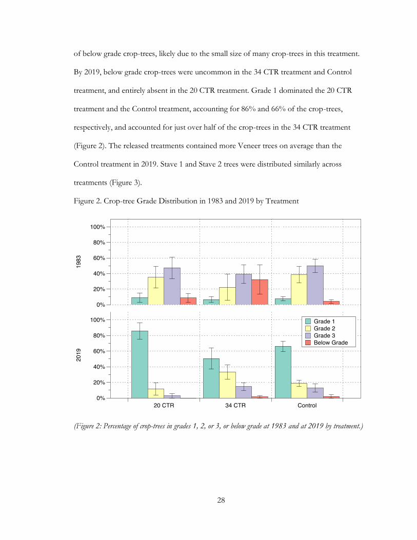
In 1983, grade 1 crop-trees were uncommon and grade 3 crop-trees were most
common across all treatments. The 34 CTR treatment contained a relatively large percentage
28
of below grade crop-trees, likely due to the small size of many crop-trees in this treatment.
By 2019, below grade crop-trees were uncommon in the 34 CTR treatment and Control
treatment, and entirely absent in the 20 CTR treatment. Grade 1 dominated the 20 CTR
treatment and the Control treatment, accounting for 86% and 66% of the crop-trees,
respectively, and accounted for just over half of the crop-trees in the 34 CTR treatment
(Figure 2). The released treatments contained more Veneer trees on average than the
Control treatment in 2019. Stave 1 and Stave 2 trees were distributed similarly across
treatments (Figure 3).
Figure 2. Crop-tree Grade Distribution in 1983 and 2019 by Treatment
(Figure 2: Percentage of crop-trees in grades 1, 2, or 3, or below grade at 1983 and at 2019 by treatment.)

29
Figure 3. Crop-tree Product Distribution in 2019 by Treatment
(Figure 3: Percentage of crop-trees in each grade and product category in 2019 by treatment. Grade 1 trees
could be assigned a Veneer, Stave 1, or Stave 2 product type, and grade 2 trees could be assigned a Stave 2
product type. The legend denotes the colors that correspond with each grade, and the labels denote the slices
that represent the product type within each grade. Slices without labels include trees within a grade that did
not qualify for a distinct product type.)

30
The proportion of crop-trees which reached their MaxPG differed by treatment
(χ2 = 34.07, P < 0.001) and by year (χ2 = 25.39, P < 0.001); however, no interaction effect
was indicated by the ANOVA. The likelihood that crop-trees in the 20 and 34 CTR
treatments would reach their maximum grade was similar, and released crop-trees were more
likely to achieve their MaxPG than unreleased crop-trees (Table 5). Across treatments, the
proportion of crop-trees reaching their MaxPG was greater in 2019 than in 1994 and 1989
(Table 6).
Table 5. Average Proportion of Crop-trees Reaching Their MaxPG by Treatment
Treatment Mean Standard Error
……………………………(%)……………………………
20 CTR 76.53a 4.29
34 CTR 78.09a 2.25
Control 55.17b 3.26
(Table 5: Average proportion expressed as a percentage (%) of crop-trees reaching their maximum potential
grade (MaxPG) by treatment. Shared subscripts (a, b) indicate no statistically significant difference; differing
subscripts indicate statistically significant difference.)

31
Table 6. Average Proportion of Crop-Trees Reaching Their MaxPG by Year
Year Mean Standard Error
……………………………(%)……………………………
1983 73.73abc 5.01
1989 59.02bc 4.23
1994 61.99bc 5.46
2001 73.36abc 4.64
2019 81.54a 4.72
(Table 6: Average proportion of crop-trees reaching their maximum potential grade (MaxPG) by year.
Shared subscripts (a, b, c) denote lack of statistical significance; differing subscripts indicate statistically
significant differences.)
4.3 Crop-tree Value
In 2019, the average butt-log value per crop-tree in the 20 CTR treatment trended
higher at $154.63, while values in the Control and 34 CTR treatments were $89.32 and
$84.32, respectively (Table 7). However, average butt-log value per crop-tree was not
statistically different among treatments [F(2, 9) = 1.38, P = 0.3].
Table 7. Average Butt-Log Value Per Crop-tree in 2019 by Treatment
Treatment Mean Value Standard Error
……………………………(USD)……………………………
20 CTR 154.63 47.28
34 CTR 84.12 28.95
Control 89.32 6.37
(Table 7: Average value (USD) per crop-tree in 2019 by treatment. Mean value refers to value calculated
using total predicted height. Mean Butt-log Value is the value calculated using the 16-foot butt-log.)

32
4.4 Stand NPV
The NPV did not vary significantly among treatments. The 20 CTR treatment
generated a marginally higher NPV at $3817.22, followed by the 34 CTR treatment at
$3570.23, and finally the Control treatment at $3499.74 (Table 8).
Table 8. Average NPV by Treatment
Treatment Mean NPV Standard Error
……………………………(USD)……………………………
20 CTR 3817.22 976.25
34 CTR 3570.23 661.17
Control 3499.74 475.98
(Table 8: Average NPV (USD) at the stand level in 2019 by treatment.)
4.5 Stand Basal Area Per Acre
An interaction effect between treatment and year showed statistical significance for
BA per acre [F(8, 45) = 2.85, P = 0.01]. Pairwise comparisons revealed that the 20 and 34
CTR treatments contained a significantly lower average BA per acre than the Control
treatment in every measurement year until 2019 (Figure 4). For the 20 CTR treatment, the
average BA per acre increased significantly among measurements separated by intervals of
10 or more years. The 34 CT treatment had identical results, except that the average BA per
acre in 1994 was not significantly larger than in 1983. The BA per acre was only larger than
previous measurements in 2019 for the Control treatment (Figure 4).

33
Figure 4. Average Basal Area Per Acre Over Time
(Figure 4: Average Basal Area (BA) per acre over time (year) by treatment; lowercase letters indicate
differences between treatments by year and uppercase letters indicate differences between years by treatment.
The letters corresponding to the 20 CTR treatment appear immediately to the right of the triangle, and those
corresponding to the 34 CTR treatment appear immediately to left of the square.)
4.6 Stand Percent Stocking
Percent stocking differed across treatments [F(2, 45) = 26.04, P < 0.001] and across
years [F(4, 45) = 41.19, P < 0.001]; however, no interaction effect occurred. The 20 and 34
CTR treatments did not differ significantly from each other in average percent stocking;
both contained lower stocking levels than the Control treatment (Table 9). In general, across
all treatments, the percent stocking became higher as time progressed, although no

34
statistically significant increase occurred between 1983-1989 or 1994-2001 (Table 10; Figure
5).
Table 9. Average Percent Stocking by Treatment
Treatment Mean Standard Error
……………………………(%)……………………………
20 CTR 92.74a 3.79
34 CTR 92.13a 4.27
Control 108.94b 2.89
(Table 9: Average percent stocking (%) by treatment. Shared subscripts (a, b) indicate no statistical
difference, while differing subscripts indicate a statistical difference.)
Table 10. Average Percent Stocking by Year
Year Mean Standard Error
……………………………(%)……………………………
1983 85.06a 3.94
1989 85.70a 4.19
1994 95.40b 2.92
2001 100.47b 3.14
2019 123.04c 2.62
(Table 10: Average percent stocking (%) by year. Shared subscript (a, b, c) denote no statistical difference;
differing subscripts denote a statistical difference exists.)

35
Figure 5. Average Percent Stocking Over Time by Treatment
(Figure 5: Average percent stocking by treatment over time)
Growth by crop-trees and ingrowth accounted for the majority of the increase in the
average percent stocking in the 34 CTR treatment from 1983 to 2019, contributing 19% and
20%, respectively (Figure 6). The contribution of non-crop-trees increased only slightly over
time for a total change of 6%. Increases in all three tree classifications contributed to the
overall percent stocking increase in the 20 CTR treatment, with crop-trees contributing 11%,
non-crop-trees 21%, and ingrowth 13%. In contrast, at 5%, the change in percent stocking
contributed by crop-trees was minimal in the Control treatment. The percent stocking of
ingrowth increased by 20% in the Control treatment from 1983 to 2019 and accounted for
nearly all of the overall percent stocking increases in this treatment (Figure 6).

36
Figure 6. Average Percent Stocking by Tree Classification Over Time by Treatment
(Figure 6: Average percent stocking by tree classification (crop-trees, non-crop-trees, ingrowth) over time by
treatment.)
For stand stocking in 1983, trees in the upper canopy (dominant and co-dominant
crown classes) contributed 29% in the 20 CTR treatment, 31% in the 34 CTR treatment, and
52% in the Control treatment of the average percent stocking. By 2019, percent stocking of
upper canopy trees was similar across treatments, increasing by 41% and 32 % in the 20
CTR and 34 CTR treatments, respectively, and by 20% in the Control treatment. The 20
CTR and 34 CTR treatments shared similar stocking levels of intermediate crown class trees,
both about 15% in 1983 and increasing to about 22% in 2019. In contrast, intermediate trees
in the Control treatment contributed 24% of the total percent stocking in 1983 and 18% in
2019. Between 1983 and 2019, the percent stocking contributed by understory (overtopped

37
crown class) trees decreased by 4% in the 20 CTR treatment, and increased by 5% and 11%
in the 34 CTR and Control treatments, respectively (Figure 7).
Figure 7. Average Percent Stocking by Crown Position Over Time by Treatment
(Figure 7: Average percent stocking by crown position including upper (dominant and co-dominant crown
classes), intermediate (intermediate crown class), and understory (overtopped crown class) over time by
treatment.)
4.7 Ingrowth
From 1983 to 2019, ingrowth contributed an average of 287.5 trees per acre in the 20
CTR treatment, 291 trees per acre in the 34 CTR treatment, and 362.5 trees per acre in the
Control treatment (Table 11). However, ingrowth density was not statistically different
among the among treatments.

38
Table 11. Average Ingrowth by Treatment
Treatment Mean Standard Error
……………………………(tpa)……………………………
20 CT 287.5 47.40
34 CT 291.0 28.41
Control 362.5 69.09
(Table 11: Average ingrowth (tpa) by treatment.)
In general, maple (Acer rubrum and Acer saccharum) dominated the ingrowth, representing on
average 42% and 35% of the ingrowth in the 20 and 34 CTR treatments respectively, and
30% in the Control treatment. Beech (Fagus grandifolia) was the second most common species
among the ingrowth, making up 35% and 22% of the ingrowth in the 20 and 34 CTR
treatments respectively, and 29% in the Control treatment. The maple and beech species
groups combined accounted for more than half of the ingrowth regardless of the treatment
(77% and 57% for the 20 and 34 CTR treatments, and 59% for the Control treatment). The
ingrowth in the Control and 34 CTR treatments also contained a substantial amount of
eastern hemlock (Tsuga canadensis), which accounted for 19% and 17% of all ingrowth,
respectively. No other species accounted for more than 10% of the total ingrowth in any
treatment (Figure 8).

39
Figure 8. Average Ingrowth by Species and Treatment
(Figure 8: Average ingrowth (%) from 1983-2019 by species and treatment.)
CHAPTER FIVE: DISCUSSION
The results of this study contribute to the body of knowledge about CTR, clarifying
aspects of the six questions offered by Trimble (1971). The study also contributes to the
information available to forest managers and landowners about promoting oak sustainability.
Despite encountering some difficulties in examining the effects of CTR on value at both the
crop-tree level and the stand level, this study suggests that CTR promotes the growth and
quality of white oak crop-trees in upland stands while stimulating growth on a stand level.
CTR also shows promise as a tool to help sustain oak-dominated forests, even on small
forestland holdings within complex management plans.

40
5.1 The Effects of Crop-tree Release on Crop-tree Growth and Quality
Fundamentally, CTR is an individual tree-focused treatment designed to increase the
diameter growth of specific trees selected to meet management objectives. Its primary
effects should be expected to be seen at the crop-tree level. The results of this study endorse
this expectation. Regardless of the number of crop-trees released per acre, the average PAI
dbh of released crop-trees was significantly greater than that of the unreleased crop-trees.
Beyond the difference in the number of crop-trees selected, the 34 CTR treatment had
smaller crop-trees on average than the 20 CTR and Control treatments. This highlights the
tree-focused nature of CTR, indicating that crop-tree density as well as crop-tree size do not
significantly alter the effects of CTR on the growth crop-trees.
Several studies note a delayed growth response following release for sawtimber red
oaks (Graney 1998; Meadows 1998; Ward 2002); however, Beck (1987) observed immediate
diameter growth of 85-year-old oaks following release. We found that the PAI dbh of white
oak crop-trees was significantly lower in the first five years (1983-1989) following release
than in the next two periods (1989-1994 and 1994-2001). While this could potentially be due
to a lag in treatment response (as observed by others), the delay likely occurred in part as a
result of a significant drought in the late 1980s. Chronic drought can reduce wood
production in deciduous forests (Brzostek et al. 2014), and in non-limiting light conditions
(such as those created by CTR), water stress has been shown to be a primary driver of
decreased relative diameter growth in white oaks (Gauthier and Jacobs 2018). From April
1987 to May 1989, the Palmer Drought Severity Index, which uses precipitation and
temperature data to estimate relative dryness, remained negative and dropped below -3
(threshold for severe drought) for the last 12 months of this period (Dai 2019) (Figure 9). A

41
drought of this length and severity offers a plausible explanation for the lag in treatment
response.
Figure 9. Palmer Drought Severity Index for Eastern Kentucky
(Figure 9: Palmer Drought Severity Index (PDSI) for Eastern Kentucky from May 1983 to September
2019. PDSI uses temperature and precipitation data to estimate relative dryness. Negative values indicate
dryness and positive values wetness. https://www7.ncdc.noaa.gov/CDO/cdo. Accessed April 2020.)
The mean crop-tree growth results provide several insights into the application of
CTR. Regarding Trimble’s first question— “At what age—or at what stage of stand development—
should a crop-tree release be made?”—the results of this study reveal that CTR can be applied to
70-80-year-old white oak dominated stands containing small sawtimber with positive growth
outcomes. Ward (2008) suggests at least 90 years as an upper limit for applying CTR,

42
reporting positive rates of growth after 12 years. Our results indicate that an upper limit of
90 years is within the realm of possibility and could potentially be exceeded. After 35 years,
PAI dbh of crop-trees slowed, likely due to decreasing space for canopy spread, and the
stand-wide percent stocking of the released treatments converged with that of the Control
treatment. This indicates that CTR applied in a small sawtimber-sized white oak dominated
stand promotes growth late into its rotation (over 100 years), highlighting the importance of
biological life span of a species and the desired product in determining whether to release a
stand. As a long-lived species associated with high value products such as veneer and stave
logs, white oak makes a good candidate for CTR late in stand development.
The per-crop-tree growth results also clarify Trimble’s second and third questions—
“How many crop-trees per acre should be selected?” and “What type of trees should be selected?”. Although
the number of crop-trees per acre that should be selected continues to depend on stand age
and development, up to 34 crop-trees per acre can be selected in small sawtimber-sized
stands. Smith et al. (1994) selected 40 and 60 black cherry or maple crop-trees per acre in a
65-year-old stand. They found that the dbh growth of crop-trees did not differ significantly
among released and unreleased crop-trees until they compared only the 40 largest crop-trees
for each plot. Considered together, these results indicate that no more than 30-40 crop-trees
per acre should be released in small sawtimber-sized stands.
Multiple studies have demonstrated that CTR significantly increases the dbh growth
of red oaks (Lamson and Smith 1978; Miller 2000; Schuler 2006; Ward 2002, 2008, 2013),
but fewer studies have examined the effects of CTR on white oak (Morrissey et al. 2011;
Sonderman 1987). Despite white oak growing slower than red oak in general (Gingrich
1967), our study demonstrates that it also responds well to CTR. Additionally, released white
oak crop-trees as small as 8.3” and as large as 18.9” in dbh grew in diameter significantly

43
more than unreleased white oak crop-trees (Miller and Stringer 2004). As to the question—
“What type of tree should be selected?”—our results support the evidence that CTR promotes dbh
growth for the white oak species and for crop-trees as small as 8” inches dbh.
One embedded uncertainty within the questions “What method should we use to release
crop-trees?; how heavy should be the release?” is how CTR affects crop-tree quality. Although crop-
trees typically respond best in terms of dbh growth to either a three- or four-sided release,
the increased light levels can cause butt-log defects such as epicormic branching. For oaks in
particular, epicormic branching can occur in CTR (Sonderman 1987), potentially reducing
butt-log quality. Dale (1968) similarly notes that epicormic branching can be severe in heavily
thinned young white oak stands, and white oak is in general prone to epicormic branching
(Miller 1996). Given these concerns, we evaluated the effect of CTR on crop-tree quality in
addition to crop-tree growth. In stark contrast to the idea that CTR might cause a loss of
quality, our results indicate that CTR improves crop-tree quality. At year 17, the number of
epicormic branches on crop-trees did not increase due to CTR (Miller and Stringer 2004).
After 35 years, regardless of the number of crop-trees released, a significantly larger
proportion of released crop-trees reached their MaxPG compared to unreleased crop-trees.
Once again, these results highlight the tree-focused nature of CTR as crop-tree density did
not alter the likelihood that a released crop-tree would reach its MaxPG.
The financial aspects of CTR are not well-documented, and we encountered several
hurdles in our financial analysis that inhibit reliable interpretation of the implications for
forest management. No difference existed among the treatments in 2019 for average per-
crop-tree value. Nevertheless, these results do not necessarily mean CTR does not increase
the dollar-value of a crop-tree. Because CTR increases the PAI dbh of a crop-tree as well as
the likelihood that a crop-tree will reach its MaxPG, the more likely financial outcome for

44
CTR is that a released crop-tree will be more valuable than if it is not released. Larger size
and better quality should translate to a more valuable crop-tree.
The size discrepancy among the treatments (the 34 CTR treatment had a significantly
smaller average dbh than the 20 CTR and Control treatments) did not mask the treatment
effects on crop-tree growth in quality, but it did undermine our ability to parse out the
management implications of the per-crop-tree value results. Size affects the value of a crop-
tree in two ways. First, it determines the volume of a crop-tree. As the volume of a crop-tree
increases, its value increases (assuming its stem quality is not reduced). Second, it determines
the grade for which a crop-tree qualifies. Whereas volume change affects crop-tree value in a
steady manner, a grade change causes a significant spike in crop-tree value. A small released
crop-tree might substantially increase in size and never cross the diameter threshold for
grade 2, while an unreleased crop-tree right at the diameter threshold for grade 2 might grow
only a little and increase substantially in value. This dynamic does not preclude the possibility
that CTR increases or maximizes the value of the small crop-tree, but it does create enough
variability in the per-crop-tree value estimates to potentially mask the treatment effect. The
discrepancy in the average stand age among treatments and the variability of site quality only
confounded the uncertainty caused by size discrepancy. Ultimately, the hurdles we
encountered reinforced the fact that the value of a tree varies with site and with the local
market. Even if we were able to assign a reliable dollar amount to a released crop-tree, this
information would be of limited use to a forester or landowner managing a different stand in
a different market.
The effect of the size discrepancy on per-crop-tree value raises a warning flag for
selecting too many crop-trees. Although site quality and stand age likely contributed to the
size discrepancy, the primary reason that the 34 CTR treatment had a smaller average crop-

45
tree diameter than the other treatments is that crop-trees that met the requirements became
increasingly difficult to find when the number increased from 20 crop-trees per acre to 34
crop-trees per acre. A compromise had to be made, and small crop-trees, some so small that
they never reached the grade 3 diameter class despite exhibiting substantial growth, had to be
released. This likely contributed to the divergence seen in crop-tree butt-log value between
the released treatments. The 20 CTR treatment had an average crop-tree butt-log value
nearly double that of the 34 CTR treatment; however, the two treatments did not
significantly differ in PAI dbh or the proportion of crop-trees reaching their MaxPG,
indicating that the divergence comes from a factor other than dbh growth or quality. The
smaller size of crop-trees in the 34 CTR treatment likely appreciably reduced the average
crop-tree value in those stands. Consistent with this theory, the 20 most valuable crop-trees
in either released treatment represent on average 70% of the total stand value per acre in
2019. The remaining 14 crop-trees per acre only increase the contribution another 7%
(Figure 10).

46
Figure 10. Percent of Total Stand Value per Acre Accounted for by Crop-trees
(Figure 10: Percent of total stand value per acre accounted for by the most valuable 6, 12, and 20 crop-trees
per acre as well as all crop-trees per acre by treatment.)
Additionally, smaller white oak crop-trees exhibited a greater proclivity for epicormic
branching than larger white oak crop-trees 17 years after release (Miller and Stringer 2004).
Although up to 34 crop-trees per acre can be released with positive outcomes for diameter
growth, selecting fewer crop-trees avoids the compromise of selecting crop-trees that might
not be worth releasing.
5.2 The Effects of Crop-tree Release on Stand Structure and Value
Although CTR is a tree-focused treatment, applying it has stand-wide implications.
For example, Ward (2017) found CTR resulted in increased upper canopy persistence and
increased diameter growth for partially released non-crop-trees. The stand-level effects of

47
CTR matter for a couple of reasons. When it comes time to harvest, the entire stand takes
precedence. Crop-trees contribute significantly to the stand, but they cease to be the sole
focus for foresters or landowners. Additionally, the widespread shift from oak-dominated
forests to late-successional forests is occurring at the stand-level not at a tree-level. When
considering any oak-focused silvicultural treatment at this point in the history of the forest
of the eastern U.S., the possibilities of the treatment to contribute to the regeneration and
recruitment of oak needs to examined.
At the outset of this study—congruent with the tree-focused nature of CTR—the
questions asked concentrated entirely on crop-trees. Concerns around oak regeneration and
recruitment were in their infancy thirty-five years ago, and questions about the effectiveness
of CTR for white oak crop-trees took precedence over questions about the ability of CTR to
preserve oak sustainability. Since then, issues concerning the regeneration and recruitment of
oak have increasingly preoccupied the world of oak silviculture. Fortunately, we were able to
ask some stand-level questions within the confines of this study.
The stand NPV per acre analysis encountered similar hurdles to the per-crop-tree
value analysis. By chance, the Control treatment tended to be older with larger diameters in
1983 than the trees in the release treatments. The variability of age and size among plots
affected the grades assigned to the non-crop-trees. A younger tree with a smaller diameter
might not qualify for a grade even if CTR positively affected the growth and quality of the
tree. The NPV per acre combines volume and grade—both of which contain underlying
issues due to tree size. Add to this the variability in site quality and age among stands, and
the NPV per acre results become difficult to interpret regarding their management
implications.

48
The basal area per acre and percent stocking provides a better picture of the
influence of CTR at a stand level. Post-treatment, both the 20 CTR and 34 CTR treatments
were significantly smaller in average BA per acre than the Control treatment. This difference
continued across time until the fifth measurement in 2019, when no significant difference
existed among treatments. These results suggest that the stands undergoing CTR grew at an
increased rate over the 35 years between the release and the end of the rotation. The average
percent stocking supports this interpretation. In 1983, after treatment, the 20 CTR and 34
CTR treatments averaged approximately 76% stocking. Prior to treatment, both treatments
were overstocked on average. The change in percent stocking due to the application of CTR
resembles the change created by a light area-wide thinning. Although CTR did not reduce
the percent stocking to the recommended 60-70% (Roach and Gingrich 1968), the
immediate environment around the crop-trees was characteristic of a lower stand density
than indicated by the percent stocking (Miller and Stringer 2004). In 2019, the released
treatments reached the upper limits of stand stocking and converged with the Control
treatment. Ingrowth contributed the majority of the total change in percent stocking for the
Control treatment. In contrast, crop-trees and non-crop-trees contributed the majority of the
total change in percent stocking in the released treatments, indicating that CTR not only
provides growing space for crop-trees but also promotes stand-wide growth.
Dey (2014) has called regeneration and recruitment the pillars of oak sustainability.
Even though CTR is not designed to address the growth and persistence of regeneration, it
has shown promise as a tool to foster oak recruitment in stands at the stem exclusion stage
(Ward 2013). In the older, small sawtimber-sized stands in this study, CTR focuses on crop-
tree growth and improvement over directly addressing oak regeneration and recruitment.
Ingrowth was strikingly similar among treatments. CTR did not cause a significant increase

49
of ingrowth, and the species composition of the ingrowth appeared similar across
treatments. Maple and beech comprise nearly half of the ingrowth in every treatment. The
one incongruence in these results is the abundance of eastern hemlock in the Control and 34
CTR treatments. Likely, site anomalies or the increased shade from more intact canopies
versus the 20 CTR treatment contributed to this.
The similarities among treatments with regards to ingrowth indicates that CTR by
itself neither promotes or diminishes oak regeneration and recruitment. Nevertheless, CTR
can contribute to oak sustainability, even in older stands. Because CTR reduces the density
of the forest canopy, it may feasibly create better light conditions for oak regeneration and
recruitment. After 15 years, the 20 CTR treatment developed twice the amount of white oak
advanced regeneration as the other treatments, and both released treatments produced
significantly taller white oak advanced regeneration than the Control treatment; however,
without addressing competition from shade-tolerant species in the understory, a harvest
would likely not regenerate white oak (Stringer 1999). Additionally, it preserves and nurtures
oak seed sources by removing competing tree species from the canopy, allowing oak
canopies to expand and thicken (Brooke et al. 2018). Rate of diameter growth has been
linked to the longevity of white oaks, and if annual dbh growth drops below 0.02 inches,
mortality rates can significantly increase (Shifley et al. 2006). Because of this, Lhotka et al.
(2016) suggest CTR as a tool to enhance the longevity of oaks in the upper canopy. As oak-
dominated forests continue to age, silvicultural treatments that reduce mortality, maintain
oak seed supply, and control stand densities will be vital to oak sustainability.
5.3 Closing Remarks
Crop-tree release applied to small sawtimber-sized upland white oak stands increases
crop-tree diameter growth as well as the likelihood that a crop-tree will reach its maximum

50
potential grade. It also stimulates stand-wide growth without altering the patterns of
ingrowth. Schuler (2006) maintains that CTR might imitate past disturbance regimes, marked
by oaks experiencing periods of suppression and release, that led to old-growth oak forests.
Research looking at CTR applied at mid- to late-rotation combined with silvicultural
treatments that focus on understory conditions (e.g. prescribed fire) would help elucidate the
potential of CTR to create canopy densities that promote oak regeneration and recruitment
given favorable understory conditions for oak. As oak-dominated forests are being replaced
by late-successional forests across the eastern U.S., landowners and foresters need
silvicultural tools that focus on active oak management.
As forestland holdings become increasingly small and forest family owners adopt a
variety of management goals, forest managers face new social complexities. CTR shows
promise in promoting active oak management within these complexities. It is scalable across
forestland sizes and across varying markets. Small-scale forestry lacks the economies of scale
and market power which large-scale forestry enjoys (Herbohn 2006). Managers and
landowners practicing forestry in small forestland holdings need silvicultural treatments that
maximize production while minimizing production costs. A commercial CTR in small-
sawtimber sized stands could achieve this, depending on local markets and stand
development. CTR also fits well within management plans with multiple objectives outside
of timber. Ward (2008) observes the aesthetic appeal of stands post-CTR and argues that
CTR is a suitable management practice for landowners who value non-commodity aspects of
their forest. Additionally, CTR meets the increased public desire for partial cutting, making it
desirable for landowners who value high forest cover (Ward 2002, 2008). Ward (2008) also
argues that CTR makes a good introduction to forest management for landowners,
highlighting another benefit of CTR—it is accessible. While traditional area-wide thinning

51
requires knowledge of stand density concepts (such as percent stocking and basal area) as
well as thinning methods (such as “thinning from below” or “crown thinning”),
understanding CTR only requires a landowner to be able to recognize a high-quality tree.
The treatment itself is also fairly straightforward: remove the trees that touch the crop-tree’s
canopy. Oak sustainability requires active-management, and the accessibility of forest
management for landowners matters. Widespread separation from the natural world
undermines the ethical and empirical foundation for stewardship (Nadkarni et al. 2017).
Perhaps the first step in sustaining oak is simply connecting landowners with their forest.

52
APPENDIX A: PRE AND POST TREATMENT TABLES

53
Table 1a. Pre-treatment Summaries and Removed Trees Summaries by Plot
Pre-treatment Removed
Plot Treatment SI Age dbh qmd tpa BA Percent
stocking Volume dbh qmd tpa BA Volume
(yr) (in) (in) (ft2) (bf) (in) (in) (ft2) (bf)
1 20 CTR 75 81 3.27 4.93 796 105.31 101.42 3329.64 12.25 12.65 38 33.17 1365.51
4 20 CTR 83 67 3.57 5.34 692 107.63 101.02 3549.90 12.36 12.93 36 32.85 1415.41
7 20 CTR 68 70 3.42 4.82 780 99.00 98.85 2239.70 8.83 9.25 36 16.80 374.14
8 20 CTR 69 65 3.81 5.18 660 96.45 95.40 2292.62 10.88 11.57 34 24.81 946.99
2 34 CTR 76 72 3.55 5.40 732 116.34 108.03 3865.97 11.64 12.27 66 54.17 2181.28
3 34 CTR 65 62 3.64 4.83 784 99.71 102.46 2057.33 9.03 9.82 54 28.42 856.78
5 34 CTR 74 52 4.20 5.06 758 105.76 111.71 1065.41 7.95 8.25 66 24.51 352.39
10 34 CTR 77 82 2.98 4.87 820 105.88 98.93 4083.22 13.00 13.33 28 27.13 1223.39
6 Control 69 70 4.13 5.77 634 115.18 108.16 3513.23 - - - - -
9 Control 69 80 3.36 5.15 738 106.85 100.50 3589.55 - - - - -
11 Control 75 99 3.18 5.07 776 108.95 101.32 4156.33 - - - - -
12 Control 77 82 4.83 6.85 422 108.07 95.26 4026.92 - - - - -
Table 12: Summaries of plots pre-treatment in 1983 and summaries of trees removed in 1983 in released plots. Variables include site index (SI, age = 50), age in years, dbh in inches, quadratic mean diameter (qmd) in inches, trees per acre (tpa), basal area (BA) per acre in square feet, percent stocking, and butt-log volume per acre in Doyle log rule board feet (bf)

54
Table 2a. Post-treatment Summaries by Plot
Post-treatment
Plot Treatment SI Age dbh qmd tpa BA Percent
stocking Volume
(yr) (in) (in) (ft2) (bf)
1 20 CTR 75 81 2.82 4.18 758 72.14 74.43 1964.12
4 20 CTR 83 67 3.09 4.57 656 74.77 74.55 2134.49
7 20 CTR 68 70 3.16 4.50 744 82.20 83.86 1865.57
8 20 CTR 69 65 3.43 4.58 626 71.64 74.87 1345.63
2 34 CTR 76 72 2.75 4.14 666 62.17 63.84 1684.69
3 34 CTR 65 62 3.24 4.23 730 71.30 77.94 1200.55
5 34 CTR 74 52 3.84 4.64 692 81.25 88.88 713.01
10 34 CTR 77 82 2.63 4.27 792 78.75 77.12 2859.83
6 Control 69 70 4.13 5.77 634 115.18 108.16 3513.23
9 Control 69 80 3.36 5.15 738 106.85 100.50 3589.55
11 Control 75 99 3.18 5.07 776 108.95 101.32 4156.33
12 Control 77 82 4.83 6.85 422 108.07 95.26 4026.92
Table 13: Summaries of plots prost-treatment in 1983. Variables include site index (SI, age = 50), age in years, dbh in inches, quadratic mean diameter (qmd) in inches, trees per acre (tpa), basal area (BA) per acre in square feet, percent stocking, and butt-log volume per acre in Doyle log rule board feet (bf)

55
Table 3a. Pre-treatment Summaries and Removed Trees Summaries by Treatment
Pre-treatment Removed
Treatment SI Age dbh qmd tpa BA Percent
stocking Volume dbh qmd tpa BA Volume
(yr) (in) (in) (ft2) (bf) (in) (in) (ft2) (bf)
20 CTR 73.75 70.75 3.52 5.07 732 102.10 99.17 2852.96 11.08 11.60 36 26.91 1025.51
34 CTR 73 67 3.59 5.04 773.5 106.92 105.28 2767.981 10.41 10.92 53.5 33.55 1153.46
Control 72.5 82.75 3.87 5.71 642.5 109.76 101.31 3821.51 - - - - -
Table 14: Pre-treatment summaries and summaries of removed trees in release treatments by treatment in 1983. Variables include site index (SI, age = 50), age in years, dbh in inches, quadratic mean diameter (qmd) in inches, trees per acre (tpa), basal area (BA) per acre in square feet, percent stocking, and butt-log volume per acre in Doyle log rule board feet (bf)
Table 4a. Post-treatment Summaries by Treatment
Post-treatment
Treatment SI Age dbh qmd tpa BA Percent
stocking Volume
(yr) (in) (in) (ft2) (bf)
20 CTR 73.75 70.75 3.12 4.46 696 75.19 76.93 1827.45
34 CTR 73 67 3.12 4.32 720 73.37 76.94 1614.52
Control 72.5 82.75 3.87 5.71 642.5 109.76 101.31 3821.51
Table 15: Post-treatment summaries by treatment in 1983. Variables include site index (SI, age = 50), age in years, dbh in inches, quadratic mean diameter (qmd) in inches, trees per acre (tpa), basal area (BA) per acre in square feet, percent stocking, and butt-log volume per acre in Doyle log rule board feet (bf)

56
APPENDIX B: CROP-TREE FIGURES AND SUMMARY STATISTICS

57
Figure 1b. Average Crop-tree Dbh (inches) by Treatment Over Time

58
Table 1b. Average Crop-tree Dbh (inches) by Treatment Over Time
Treatment Year Min 1st Quartile Median 3rd Quartile Max Mean SD
20 CTR
1983 11.37 12.05 13.37 14.74 15.56 13.42 1.93
1989 12.02 12.81 14.23 15.64 16.38 14.21 2.02
1994 12.96 13.89 15.54 17.02 17.44 15.37 2.14
2001 14.19 15.19 16.99 18.48 18.56 16.68 2.18
2019 16.59 18.07 20.17 21.78 21.80 19.68 2.56
34 CTR
1983 9.04 9.51 11.29 13.34 14.65 11.57 2.66
1989 9.67 10.24 12.00 14.01 15.32 12.25 2.66
1994 10.62 11.28 13.03 15.00 16.33 13.25 2.66
2001 12.00 12.45 14.14 16.16 17.62 14.47 2.64
2019 14.33 15.26 17.18 19.15 20.19 17.22 2.73
Control
1983 13.43 13.75 14.08 14.31 14.31 13.97 0.42
1989 14.10 14.29 14.55 14.78 14.86 14.52 0.35
1994 14.99 15.12 15.37 15.60 15.70 15.35 0.33
2001 15.88 16.29 16.52 16.63 16.74 16.41 0.38
2019 17.61 18.21 18.75 19.15 19.31 18.61 0.77

59
Figure 2b. Average Crop-tree Quadratic Mean Diameter (inches) by Treatment Over Time

60
Table 2b. Average Crop-Tree Quadratic Mean Diameter (inches) by Treatment Over Time
Treatment Year Min 1st Quartile Median 3rd Quartile Max Mean SD
20 CTR
1983 11.50 12.16 13.55 15.03 15.97 13.64 2.06
1989 12.15 12.91 14.38 15.88 16.75 14.41 2.13
1994 13.09 13.98 15.66 17.22 17.77 15.54 2.22
2001 14.32 15.28 17.08 18.64 18.87 16.84 2.23
2019 16.74 18.18 20.27 21.91 21.98 19.82 2.57
34 CTR
1983 9.15 9.76 11.52 13.49 14.75 11.73 2.63
1989 9.76 10.45 12.22 14.17 15.42 12.40 2.63
1994 10.72 11.47 13.23 15.17 16.44 13.41 2.65
2001 12.11 12.65 14.34 16.33 17.74 14.64 2.63
2019 14.47 15.47 17.40 19.33 20.33 17.40 2.72
Control
1983 13.79 14.01 14.24 14.41 14.44 14.18 0.30
1989 14.46 14.56 14.74 14.90 14.94 14.72 0.23
1994 15.24 15.46 15.61 15.70 15.77 15.56 0.24
2001 16.13 16.56 16.74 16.79 16.81 16.61 0.32
2019 17.90 18.35 18.84 19.30 19.65 18.81 0.77

61
Figure 3b. Basal Area (ft2) Per Acre of Crop-trees by Treatment Over Time

62
Table 3b. Basal Area (ft2) Per Acre of Crop-trees by Treatment Over Time
Treatment Year Min 1st Quartile Median 3rd Quartile Max Mean SD
20 CTR
1983 12.99 13.28 17.32 21.52 22.27 17.48 4.97
1989 14.48 14.97 19.50 24.02 24.50 19.49 5.42
1994 16.81 17.55 22.68 27.79 28.48 22.66 6.21
2001 20.13 20.97 26.16 31.75 33.82 26.57 6.89
2019 27.51 29.65 36.27 43.38 47.03 36.77 9.33
34 CTR
1983 14.60 15.82 23.96 32.08 33.22 23.94 9.88
1989 16.64 18.17 26.87 35.37 36.30 26.67 10.45
1994 20.07 21.89 31.39 40.54 41.28 31.03 11.31
2001 25.61 26.58 36.79 47.02 48.05 36.81 12.21
2019 36.54 39.81 52.02 64.08 66.87 51.86 15.36
Control
1983 18.08 23.18 24.94 25.25 25.98 23.49 3.64
1989 19.47 24.82 26.99 27.50 27.86 25.33 3.94
1994 21.71 27.56 29.95 30.69 31.58 28.30 4.47
2001 24.67 31.26 33.76 34.78 36.89 32.27 5.28
2019 32.11 38.83 41.52 44.11 50.55 41.42 7.54

63
Figure 4b. Percent Stocking of Crop-trees by Treatment Over Time

64
Table 4b. Percent Stocking of Crop-trees by Treatment Over Time
Treatment Year Min 1st Quartile Median 3rd Quartile Max Mean SD
20 CTR
1983 10.93 11.01 13.86 16.79 17.09 13.94 3.42
1989 12.00 12.20 15.37 18.51 18.61 15.34 3.70
1994 13.64 14.00 17.40 20.91 21.62 17.51 4.22
2001 15.95 16.35 19.75 23.56 25.21 20.16 4.65
2019 20.97 22.20 26.48 31.23 33.90 26.96 6.18
34 CTR
1983 13.24 13.96 19.95 25.81 26.13 19.82 7.06
1989 14.76 15.70 22.03 28.09 28.24 21.76 7.38
1994 17.27 18.40 25.20 31.62 31.65 24.83 7.88
2001 21.24 21.74 28.95 36.04 36.16 28.83 8.38
2019 28.86 30.88 38.85 47.01 49.55 39.03 10.34
Control
1983 14.32 18.40 19.79 20.01 20.62 18.63 2.90
1989 15.27 19.46 21.20 21.63 21.92 19.90 3.12
1994 16.80 21.34 23.25 23.84 24.41 21.93 3.48
2001 18.81 23.85 25.84 26.62 28.02 24.63 4.02
2019 23.77 28.92 31.04 32.86 37.13 30.74 5.47

65
Figure 5b. Butt-log Volume (board feet, Doyle) Per Crop-tree by Treatment Over Time

66
Table 5b. Butt-log Volume (board feet, Doyle) Per Crop-tree by Treatment Over Time
Treatment Year Min 1st Quartile Median 3rd Quartile Max Mean SD
20 CTR
1983 30.67 32.50 46.00 63.17 76.04 49.68 21.72
1989 33.78 38.97 55.16 73.93 86.86 57.74 24.86
1994 40.02 49.55 71.15 92.70 102.09 71.10 29.47
2001 53.46 65.16 91.33 115.20 120.04 89.04 32.81
2019 85.26 107.67 145.75 177.04 179.10 138.97 46.41
34 CTR
1983 18.55 27.28 35.17 44.68 58.30 36.80 16.83
1989 19.04 26.74 38.28 52.12 66.73 40.58 20.97
1994 24.93 31.16 45.97 64.21 80.70 49.39 25.34
2001 33.90 40.13 57.70 79.97 100.28 62.40 30.40
2019 55.25 68.41 97.13 127.53 145.72 98.81 41.98
Control
1983 52.72 53.71 54.42 55.00 55.59 54.29 1.22
1989 60.25 60.45 60.68 61.09 61.86 60.87 0.71
1994 69.83 70.19 70.43 70.73 71.28 70.49 0.61
2001 83.44 84.11 85.12 86.23 87.19 85.22 1.66
2019 103.98 110.41 118.38 126.69 134.16 118.72 13.21

67
Figure 6b. Butt-log Volume (board feet, Doyle) Per Acre of Crop-trees by Treatment Over
Time

68
Table 6b. Butt-log Volume (board feet, Doyle) Per Acre of Crop-trees by Treatment over
Time
Treatment Year Min 1st Quartile Median 3rd Quartile Max Mean SD
20 CTR
1983 429.32 504.70 794.88 1099.11 1216.63 808.93 387.83
1989 540.49 623.51 952.13 1287.24 1389.73 958.62 425.01
1994 720.32 812.86 1228.03 1617.63 1633.46 1202.46 488.17
2001 962.24 1069.36 1512.83 1951.60 2044.62 1508.13 553.29
2019 1534.62 1765.41 2354.00 2942.85 3174.43 2354.26 789.11
34 CTR
1983 185.48 318.12 863.55 1431.67 1632.37 886.24 719.09
1989 342.68 481.27 1066.95 1671.93 1868.45 1086.26 763.23
1994 548.41 735.34 1396.89 2061.97 2259.48 1400.42 852.86
2001 949.21 1060.30 1793.11 2568.66 2807.95 1835.85 949.21
2019 1768.01 2079.81 3131.91 4092.56 4129.99 3040.46 1241.10
Control
1983 864.65 1086.08 1182.74 1209.93 1222.95 1113.27 167.87
1989 968.26 1236.18 1331.97 1344.08 1360.95 1248.29 187.26
1994 1140.47 1445.21 1549.48 1583.09 1675.85 1478.82 233.31
2001 1374.46 1720.36 1845.50 1914.65 2092.58 1789.51 300.32
2019 1987.16 2354.02 2485.89 2676.56 3219.82 2544.69 507.85

69
APPENDIX C: STAND FIGURES AND SUMMARY STATISTICS

70
Figure 1c. Trees Per Acre by Treatment over Time

71
Table 1c. Trees Per Acre by Treatment over Time
Treatment Year Min 1st Quartile Median 3rd Quartile Max Mean SD
20 CTR
1983 626 648.5 700 747.5 758 696 64.93
1989 530 591.5 644 679 688 626.5 72.47
1994 622 703 763 805.5 834 745.5 92.87
2001 604 604 641 689.5 724 652.5 59.07
2019 482 564.5 612 641 668 593.5 80.55
34 CTR
1983 666 685.5 711 745.5 792 720 54.72
1989 572 590 643 696 714 643 69.52
1994 644 824 888 909 960 845 138.27
2001 636 726 766 782 800 742 72.92
2019 476 536 589 639.5 692 586.5 92.25
Control
1983 422 581 686 747.5 776 642.5 158.78
1989 418 526 651 752 788 627 169.90
1994 468 549 672 803.5 910 680.5 196.98
2001 448 557.5 599 644.5 766 603 129.97
2019 446 563 620 677 794 620 142.83

72
Figure 2c. Cumulative Ingrowth (TPA) by Treatment Over Time

73
Table 2c. Cumulative Ingrowth (TPA) by Treatment Over Time
Treatment Year Min 1st Quartile Median 3rd Quartile Max Mean SD
20 CTR
1983 0 0 0 0 0 0 0
1989 12 36 47 55 70 44 24
1994 150 150 204 269 300 215 76
2001 212 242 281 330 390 291 77
2019 338 467 516 533 564 484 100
34 CTR
1983 0 0 0 0 0 0 0
1989 12 36 53 64 68 47 25
1994 156 281 345 375 394 310 107
2001 238 366 429 455 468 391 105
2019 480 483 522 576 624 537 69
Control
1983 0 0 0 0 0 0 0
1989 14 23 31 54 106 46 41
1994 128 155 171 207 294 191 72
2001 166 202 320 429 438 311 141
2019 332 415 565 701 738 550 195

74
Figure 3c. Cumulative Mortality (TPA) by Treatment Over Time

75
Table 3c. Cumulative Mortality (TPA) by Treatment Over Time
Treatment Year Min 1st Quartile Median 3rd Quartile Max Mean SD
20 CTR
1983 0.00 0.00 0.00 0.00 0.00 0.00 0.00
1989 92.00 101.00 105.00 108.00 114.00 104.00 9.09
1994 138.00 144.00 150.00 157.00 166.00 151.00 11.94
2001 202.00 217.00 238.00 260.50 280.00 239.50 34.46
2019 292.00 319.00 342.00 364.50 390.00 341.50 41.61
34 CTR
1983 0.00 0.00 0.00 0.00 0.00 0.00 0.00
1989 82.00 109.00 123.00 129.00 132.00 115.00 22.77
1994 150.00 160.50 171.00 182.00 194.00 171.50 18.86
2001 228.00 240.00 264.00 293.00 320.00 269.00 41.36
2019 318.00 325.50 367.00 417.00 450.00 375.50 63.36
Control
1983 0.00 0.00 0.00 0.00 0.00 0.00 0.00
1989 40.00 49.00 53.00 60.50 80.00 56.50 16.84
1994 106.00 118.00 138.00 160.50 180.00 140.50 33.04
2001 198.00 241.50 258.00 274.50 318.00 258.00 49.02
2019 256.00 313.00 361.00 404.50 448.00 356.50 82.05

76
Figure 4c. Average Dbh (inches) by Treatment Over Time

77
Table 4c. Average Dbh (inches) by Treatment Over Time
Treatment Year Min 1st Quartile Median 3rd Quartile Max Mean SD
20 CTR
1983 2.82 3.02 3.12 3.22 3.43 3.12 0.25
1989 3.26 3.33 3.35 3.49 3.92 3.47 0.30
1994 3.26 3.33 3.42 3.54 3.73 3.46 0.20
2001 3.75 3.80 3.85 3.90 3.96 3.85 0.09
2019 4.11 4.39 4.52 4.75 5.35 4.62 0.52
34 CTR
1983 2.63 2.72 3.00 3.39 3.84 3.12 0.55
1989 2.79 2.93 3.25 3.70 4.26 3.39 0.66
1994 2.81 2.82 3.08 3.52 4.06 3.26 0.59
2001 3.38 3.50 3.63 3.88 4.37 3.75 0.44
2019 4.29 4.58 4.82 5.04 5.25 4.80 0.41
Control
1983 3.18 3.32 3.74 4.30 4.83 3.87 0.76
1989 3.33 3.37 3.89 4.52 4.91 4.00 0.77
1994 3.32 3.39 3.80 4.29 4.56 3.87 0.60
2001 3.75 3.91 4.10 4.36 4.70 4.17 0.41
2019 4.22 4.23 4.26 4.55 5.31 4.51 0.53

78
Figure 5c. Quadratic Mean Diameter (inches) by Treatment Over Time

79
Table 5c. Quadratic Mean Diameter (inches) by Treatment Over Time
Treatment Year Min 1st Quartile Median 3rd Quartile Max Mean SD
20 CTR
1983 4.18 4.42 4.54 4.57 4.58 4.46 0.19
1989 4.66 4.70 4.74 4.86 5.12 4.82 0.21
1994 4.59 4.73 4.86 4.96 5.03 4.83 0.19
2001 5.15 5.27 5.33 5.40 5.53 5.34 0.15
2019 5.78 6.12 6.44 6.83 7.39 6.51 0.68
34 CTR
1983 4.14 4.21 4.25 4.36 4.64 4.32 0.22
1989 4.23 4.32 4.46 4.70 5.12 4.57 0.39
1994 4.05 4.10 4.29 4.62 5.12 4.44 0.49
2001 4.76 4.93 5.00 5.16 5.58 5.09 0.35
2019 5.78 6.27 6.60 6.79 6.88 6.46 0.50
Control
1983 5.07 5.13 5.46 6.04 6.85 5.71 0.82
1989 5.14 5.28 5.71 6.32 7.00 5.89 0.85
1994 5.08 5.27 5.64 6.14 6.74 5.77 0.74
2001 5.84 5.84 6.11 6.44 6.62 6.17 0.39
2019 6.08 6.22 6.35 6.72 7.55 6.58 0.66

80
Figure 6c. Basal Area (ft2) Per Acre by Treatment Over Time

81
Table 6c. Basal Area (ft2) Per Acre by Treatment Over Time
Treatment Year Min 1st Quartile Median 3rd Quartile Max Mean SD
20 CTR
1983 71.64 72.01 73.46 76.63 82.20 75.19 4.87
1989 75.81 76.04 78.87 81.71 81.96 78.88 3.37
1994 85.79 93.39 96.41 97.44 99.10 94.43 5.91
2001 94.55 97.28 99.42 103.31 111.30 101.17 7.20
2019 121.65 130.73 138.22 142.86 143.43 135.38 10.15
34 CTR
1983 62.17 69.02 75.02 79.37 81.25 73.37 8.58
1989 61.50 67.65 74.09 79.31 81.78 72.87 9.13
1994 79.97 86.45 90.32 92.99 95.82 89.11 6.77
2001 93.47 103.25 107.28 108.12 108.28 104.08 7.12
2019 122.99 125.19 132.26 139.09 140.55 132.02 8.85
Control
1983 106.85 107.76 108.51 110.51 115.18 109.76 3.72
1989 111.83 113.16 113.79 114.05 114.26 113.42 1.09
1994 110.77 114.60 117.51 121.42 128.24 118.51 7.35
2001 107.23 111.13 122.25 134.70 142.61 123.58 16.59
2019 136.10 136.55 137.76 144.11 159.97 142.90 11.44

82
Figure 7c. Percent Stocking by Treatment Over Time

83
Table 7c. Percent Stocking by Treatment Over Time
Treatment Year Min 1st Quartile Median 3rd Quartile Max Mean SD
20 CTR
1983 74.43 74.52 74.71 77.12 83.86 76.93 4.63
1989 75.95 76.44 79.35 82.23 82.61 79.32 3.53
1994 86.13 93.35 96.75 98.05 98.96 94.65 5.83
2001 92.45 94.56 96.38 99.90 107.13 98.09 6.37
2019 113.91 120.49 123.68 124.91 125.63 121.72 5.35
34 CTR
1983 63.84 73.80 77.53 80.67 88.88 76.95 10.25
1989 62.82 68.76 77.05 84.01 85.96 75.72 10.87
1994 84.45 90.56 93.61 96.31 101.37 93.26 6.97
2001 93.88 101.88 105.69 107.46 109.37 103.66 6.81
2019 109.35 117.43 123.71 127.47 127.99 121.19 8.66
Control
1983 95.26 99.19 100.91 103.03 108.16 101.31 5.30
1989 97.70 103.35 105.25 105.61 106.64 103.71 4.06
1994 101.22 102.19 106.16 112.68 121.26 108.70 9.19
2001 95.81 99.53 108.68 120.07 130.52 110.92 15.79
2019 118.61 119.64 120.98 127.96 145.94 126.63 12.95
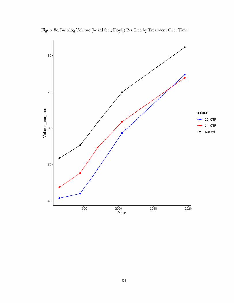
84
Figure 8c. Butt-log Volume (board feet, Doyle) Per Tree by Treatment Over Time

85
Table 8c. Butt-log Volume (board feet, Doyle) Per Tree by Treatment Over Time
Treatment Year Min 1st Quartile Median 3rd Quartile Max Mean SD
20 CTR
1983 33.31 33.56 39.05 46.27 51.69 40.78 8.93
1989 35.93 36.10 41.88 47.84 48.54 42.06 6.96
1994 39.79 40.69 48.88 56.91 57.30 48.71 9.63
2001 43.73 48.83 60.32 70.15 70.29 58.66 13.60
2019 55.71 68.98 76.92 82.66 89.35 74.72 14.26
34 CTR
1983 32.41 34.43 44.03 53.36 54.57 43.76 11.62
1989 29.85 39.16 47.71 56.26 65.58 47.71 15.25
1994 33.90 47.74 53.31 60.27 78.26 54.70 18.20
2001 39.08 51.96 58.12 67.95 91.82 61.79 21.99
2019 47.01 55.33 73.87 92.42 100.74 73.87 25.44
Control
1983 47.23 47.41 50.23 54.58 59.38 51.77 5.73
1989 51.38 51.67 54.67 58.33 60.58 55.33 4.51
1994 54.76 56.76 61.50 66.34 68.59 61.59 6.56
2001 63.97 67.55 69.20 71.57 77.33 69.92 5.53
2019 69.78 79.74 83.07 85.58 93.08 82.25 9.56

86
Figure 9c. Butt-log Volume (board feet, Doyle) Per Acre by Treatment Over Time

87
Table 9c. Butt-log Volume (board feet, Doyle) Per Acre by Treatment Over Time
Treatment Year Min 1st Quartile Median 3rd
Quartile Max Mean SD
20 CTR
1983 1345.63 1735.58 1914.85 2006.72 2134.49 1827.45 339.88
1989 1591.02 1906.99 2122.65 2293.66 2475.64 2077.99 375.77
1994 1989.72 2341.75 2762.49 3072.97 3094.20 2652.23 529.99
2001 2536.48 2604.75 3141.29 3687.68 3785.54 3151.15 660.40
2019 3899.81 4498.18 5386.75 6085.09 6112.78 5196.52 1086.76
34 CTR
1983 713.02 1078.67 1442.62 1978.47 2859.83 1614.52 920.11
1989 1014.85 1370.02 1673.92 2017.61 2492.13 1713.71 623.52
1994 1423.89 1821.21 2128.63 2471.15 2973.77 2163.73 649.93
2001 2188.50 2572.41 2789.94 3077.78 3672.66 2860.26 615.68
2019 3290.52 4134.35 4628.31 4890.02 5037.07 4396.05 781.34
Control
1983 3513.23 3570.47 3808.24 4059.27 4156.33 3821.51 317.88
1989 3699.64 3953.30 4207.01 4433.15 4604.10 4179.44 395.51
1994 3833.31 4489.68 4715.28 4776.25 4938.72 4550.65 489.72
2001 4124.87 4478.77 5113.01 5691.21 5877.01 5056.97 832.79
2019 5582.44 5863.50 6051.70 6188.17 6314.03 5999.97 314.21

88
APPENDIX D: ANOVA TABLES

89
Table 1d. Type III Anova for Avg. Dbh of Crop-trees
Parameter Df Sum Sq F value P value
Treatment 2 57.300 7.097 0.002
Year 4 226.600 14.038 <0.001
Treatment:Year 8 3.200 0.100 0.999
Residuals 45 181.600
Table 2d. Tukey Pairwise Comparisons of Avg. Dbh of Crop-trees among Treatments
Contrast Estimate SE Df T ratio P value
20CTR – 34
CTR
2.120 0.635 45 3.338 0.005
20 CTR –
Control
0.100 0.635 45 0.157 0.987
34 CTR -
Control
-2.021 0.635 45 -3.182 0.007

90
Table 3d. Tukey Pairwise Comparisons of Avg. Dbh of Crop-trees among Years
Contrast Estimate SE Df T ratio P value
1983 – 1989 -0.673 0.82 45 -0.821 0.923
1983 – 1994 -1.672 0.82 45 -2.039 0.265
1983 – 2001 -2.869 0.82 45 -3.499 0.009
1983 – 2019 -5.516 0.82 45 -6.727 <0.001
1989 – 1994 -0.999 0.82 45 -1.218 0.741
1989 – 2001 -2.196 0.82 45 -2.678 0.073
1989 – 2019 -4.843 0.82 45 -5.906 <0.001
1994 – 2001 -1.197 0.82 45 -1.460 0.593
1994 – 2019 -3.844 0.82 45 -4.688 <0.001
2001 – 2019 -2.647 0.82 45 -3.228 0.019
Table 4d. Type III Anova for PAI Dbh of Crop-trees
Parameter Df Sum Sq F value P value
Treatment 2 0.019 14.399 <0.001
Period 3 0.030 14.788 <0.001
Treatment:Period 6 0.001 0.211 0.971
Residuals 36 0.024

91
Table 5d. Tukey Pairwise Comparisons of PAI Dbh of Crop-trees among Treatments
Contrast Estimate SE Df T ratio P value
20CTR – 34
CTR
0.020 0.009 36 2.204 0.084
20 CTR –
Control
0.049 0.009 36 5.399 <0.001
34 CTR -
Control
0.029 0.009 36 3.135 0.009
Table 6d. Tukey Pairwise Comparisons of PAI Dbh of Crop-trees among Periods
Contrast Estimate SE Df T ratio P value
1983 to 1989 – 1989 to
1994
-0.065 0.011 36 -6.166 <0.001
1983 to 1989 – 1994 to
2001
-0.036 0.011 36 -3.442 0.008
1983 to 1989 – 2001 to
2019
-0.012 0.011 36 -1.174 0.647
1994 to 2001 – 1989 to
1994
-0.029 0.011 36 -2.724 0.047
1994 to 2001 – 2001 to
2019
0.024 0.011 36 2.268 0.125
2001 to 2019 – 1989 to
1994
-0.053 0.011 36 -4.992 <0.001

92
Table 7d. Type III Anova for MaxPG of Crop-trees
Parameter Df Chi square P value
Treatment 2 34.073 <0.001
Year 4 25.393 <0.001
Treatment:Year 8 13.342 0.101
Table 8d. Tukey Pairwise Comparisons of MaxPG of Crop-trees among Treatments
Estimates are given on the logs odds ratio scale.
Contrast Estimate SE Z ratio P value
20CTR – 34 CTR 0.184 0.293 0.626 0.806
20 CTR – Control 1.209 0.294 4.114 <0.001
34 CTR - Control 1.026 0.198 5.173 <0.001

93
Table 9d. Tukey Pairwise Comparisons of MaxPG of Crop-trees among Years.
Estimates are given on the logs odds ratio scale.
Contrast Estimate SE Z ratio P value
1983 – 1989 0.761 0.281 2.704 0.053
1983 – 1994 0.585 0.285 2.054 0.241
1983 – 2001 0.074 0.297 0.250 0.999
1983 – 2019 -0.741 0.429 -1.727 0.417
1989 – 1994 -0.176 0.261 -0.673 0.962
1989 – 2001 -0.687 0.274 -2.510 0.088
1989 – 2019 -1.502 0.413 -3.635 0.003
1994 – 2001 -0.511 0.277 -1.843 0.349
1994 – 2019 -1.326 0.416 -3.191 0.012
2001 – 2019 -0.815 0.424 -1.923 0.305
Table 10d. Type III Anova for Mean Butt-log Value of Crop-trees
Parameter Df Sum Sq F value P value
Treatment 2 6854 0.723 0.511
Residuals 9 42652
Table 11d. Type III Anova for Stand NPV Per Acre
Parameter Df Sum Sq F value P value
Treatment 2 222352 0.052 0.950
Residuals 9 19401220

94
Table 12d. Type III Anova for Stand BA Per Acre
Parameter Df Sum Sq F value P value
Treatment 2 9154 69.317 <0.001
Year 4 20090 76.064 <0.001
Treatment:Year 8 1505 2.850 0.012
Residuals 45 2971
Table 13d. Tukey Pairwise Comparisons of Stand BA Per Acre among Treatments in Year
1983
Contrast Estimate SE Df T ratio P value
20 CTR – 34
CTR
1.82 5.75 45 0.317 0.946
20 CTR -
Control
-34.58 5.75 45 -6.017 <0.001
34 CTR -
Control
-36.40 5.75 45 -6.334 <0.001
Table 14d. Tukey Pairwise Comparisons of Stand BA Per Acre among Treatments in Year
1989
Contrast Estimate SE Df T ratio P value
20 CTR – 34
CTR
6.14 5.75 45 1.069 0.538
20 CTR -
Control
-34.55 5.75 45 -6.013 <0.001

95
34 CTR -
Control
-40.69 5.75 45 -7.082 <0.001
Table 15d. Tukey Pairwise Comparisons of Stand BA Per Acre among Treatments in Year
1994
Contrast Estimate SE Df T ratio P value
20 CTR – 34
CTR
6.19 5.75 45 1.077 0.533
20 CTR -
Control
-23.85 5.75 45 -4.150 <0.001
34 CTR -
Control
-30.03 5.75 45 -5.227 <0.001
Table 16d. Tukey Pairwise Comparisons of Stand BA Per Acre among Treatments in Year
2001
Contrast Estimate SE Df T ratio P value
20 CTR – 34
CTR
-2.23 5.75 45 -0.287 0.921
20 CTR -
Control
-22.03 5.75 45 -3.834 0.001
34 CTR -
Control
-19.80 5.75 45 -3.446 0.004

96
Table 17d. Tukey Pairwise Comparisons of Stand BA Per Acre among Treatments in Year
2019
Contrast Estimate SE Df T ratio P value
20 CTR – 34
CTR
3.34 5.75 45 0.581 0.831
20 CTR -
Control
-7.71 5.75 45 -1.342 0.380
34 CTR -
Control
-11.05 5.75 45 -1.923 0.144
Table 18d. Tukey Pairwise Comparisons of Stand BA Per Acre among Years for the 20 CTR
Treatment
Contrast Estimate SE Df T ratio P value
1983 – 1989 -3.488 5.75 45 -0.626 0.973
1983 – 1994 -17.820 5.75 45 -3.101 0.026
1983 – 2001 -24.238 5.75 45 -4.218 0.001
1983 – 2019 -59.997 5.75 45 -10.442 <0.001
1989 – 1994 -14.332 5.75 45 -2.494 0.110
1989 – 2001 -20.750 5.75 45 -3.611 0.007
1989 – 2019 -56.510 5.75 45 -9.835 <0.001
1994 – 2001 -6.418 5.75 45 -1.117 0.797
1994 – 2019 -42.177 5.75 45 -7.340 <0.001
2001 – 2019 -35.759 5.75 45 -6.223 <0.001

97
Table 19d. Tukey Pairwise Comparisons of Stand BA Per Acre among Years for the 34 CTR
Treatment
Contrast Estimate SE Df T ratio P value
1983 – 1989 0.834 5.75 45 0.145 1.000
1983 – 1994 -13.453 5.75 45 -2.341 0.151
1983 – 2001 -28.284 5.75 45 -4.922 <0.001
1983 – 2019 -58.483 5.75 45 -10.178 <0.001
1989 – 1994 -14.287 5.75 45 -2.487 0.111
1989 – 2001 -29.118 5.75 45 -5.068 <0.001
1989 – 2019 -59.316 5.75 45 -10.323 <0.001
1994 – 2001 -14.831 5.75 45 -2.581 0.091
1994 – 2019 -45.029 5.75 45 -7.837 <0.001
2001 – 2019 -30.199 5.75 45 -5.256 <0.001

98
Table 20d. Tukey Pairwise Comparisons of Stand BA Per Acre among Years for the Control
Treatment
Contrast Estimate SE Df T ratio P value
1983 – 1989 -3.462 5.75 45 -0.602 0.974
1983 – 1994 -7.091 5.75 45 -1.234 0.732
1983 – 2001 -11.691 5.75 45 -2.035 0.267
1983 – 2019 -33.136 5.75 45 -5.767 <0.001
1989 – 1994 -3.630 5.75 45 -0.632 0.969
1989 – 2001 -8.229 5.75 45 -1.432 0.611
1989 – 2019 -29.674 5.75 45 -5.164 <0.001
1994 – 2001 -4.600 5.75 45 -0.800 0.929
1994 – 2019 -26.045 5.75 45 -4.533 <0.001
2001 – 2019 -21.445 5.75 45 -3.732 0.005
Table 21d. Type III Anova for Stand Percent Stocking
Parameter Df Sum Sq F value P value
Treatment 2 3636 26.040 <0.001
Year 4 11503 41.195 <0.001
Treatment:Year 8 921 1.649 0.138
Residuals 45 3141

99
Table 22d. Tukey Pairwise Comparisons of Percent Stocking among Treatments
Contrast Estimate SE Df T ratio P value
20CTR – 34
CTR
0.61 2.64 45 0.231 0.971
20 CTR –
Control
-16.20 2.64 45 -6.131 <0.001
34 CTR -
Control
-16.81 2.64 45 -6.362 <0.001
Table 23d. Tukey Pairwise Comparisons of Percent Stocking among Years
Contrast Estimate SE Df T ratio P value
1983 – 1989 -0.644 3.41 45 -0.189 1.000
1983 – 1994 -10.345 3.41 45 -3.033 0.031
1983 – 2001 -15.412 3.41 45 -4.518 <0.001
1983 – 2019 -37.982 3.41 45 -11.135 <0.001
1989 – 1994 -9.701 3.41 45 -2.844 0.050
1989 – 2001 -14.768 3.41 45 -4.330 <0.001
1989 – 2019 -37.339 3.41 45 -10.947 <0.001
1994 – 2001 -5.067 3.41 45 -1.486 0.577
1994 – 2019 -27.638 3.41 45 -8.103 <0.001
2001 – 2019 -22.570 3.41 45 -6.617 <0.001

100
Table 24d. Type III Anova for Stand Ingrowth Per Acre
Parameter Df Sum Sq F value P value
Treatment 2 14333 0.687 0.528
Residuals 9 93922

101
APPENDIX E: R CODE

102
## Title: CTR Master Code
# Author: Philip Vogel
# Created: April 22, 2020
pkgs <- c("nlme", "car", "lme4", "emmeans", "ggplot2", "tidyverse")
for(i in 1:length(pkgs)) {
if(pkgs[i] %in% installed.packages()) {
require(pkgs[i], character.only = T)
} else {
install.packages(pkgs[i])
require(pkgs[i], character.only = T)
}
}
# Import CSV ----------------------------------------------------------
----
#import ctr_full csv
ctr <- read_csv("ctr_full.csv",
col_types = cols(
Order=col_double(),
Plot=col_factor(),
Treatment=col_factor(),
ID=col_double(),
Species.Name=col_character(),
Cropcut=col_factor(),
Classification=col_character(),
Damage=col_factor(),
Severity=col_factor(),
CC0=col_double(),
CC5=col_double(),
CC10=col_double(),
CC17=col_double(),
CC35=col_double(),
PREDBH=col_double(),
DBH0=col_double(),
DBH5=col_double(),
DBH10=col_double(),
DBH17=col_double(),
DBH35=col_double(),
G0=col_double(),
G5=col_double(),
G10=col_double(),
G17=col_double(),
G35=col_double(),
MORT0=col_double(),
MORT5=col_double(),
MORT10=col_double(),
MORT17=col_double(),
MORT35=col_double(),
STEMS0=col_double(),
STEMS5=col_double(),
STEMS10=col_double(),
STEMS17=col_double(),
STEMS35=col_double(),
REMARKS0=col_character(),

103
REMARKS5=col_character(),
REMARKS10=col_character(),
REMARKS17=col_character(),
REMARKS35=col_character()
))
#rename treatment factors
ctr$Treatment <- ifelse(ctr$Treatment==1, "20_CTR",
ifelse(ctr$Treatment==2, "34_CTR",
"Control"))
#import si.age csv
SI.AGE <- read_csv("si_age.csv",
col_types=cols(
Plot=col_factor()
))
# Load CTR Functions ####
mesavage = function( dbh, mht, volumetype="Int1/4", girard=78)
{
# Function to calcalate the Mesavage and Girard 1946 volume.
# using the equations by H.V. Wiant, Jr., 1986, Formula's for
# Mesavage and Girard's Volume Tables, Northern Journal of Applied
Forestry 3:124.
# Coded by David R. Larsen, June 20, 2015
L = mht / 16.0
cor = (1.0+ ((girard - 78.0) * 0.03))
a = vector()
b = vector()
c = vector()
treevolume=numeric()
if (volumetype == "Int1/4"){
a = c(-13.35212, 9.58615, 1.52968)
b = c(1.79620, -2.59995, -0.27465)
c = c(0.04482, 0.45997, -0.00961)
}else if (volumetype == "Scribner"){
a = c(-22.50365, 17.53508, -0.59242)
b = c(3.02888, -4.34381, -0.02302)
c = c(-0.01969, 0.51593, -0.02035)
}else if (volumetype == "Doyle"){
a = c(-29.37337, 41.51275, 0.55743)
b = c(2.78043, -8.77272, -0.04516)
c = c(0.04177, 0.59042, -0.01578)
}else{
cat("volumetype not found!")
}
v1 = (a[1] + a[2] * L + a[3] * L**2)
v2 = (b[1] + b[2] * L + b[3] * L**2) * dbh
v3 = (c[1] + c[2] * L + c[3] * L**2) * dbh**2
volume = (v1 + v2 + v3) * cor
volume
}

104
#function for basal area per acre using dbh
#the total sum of the constant k multiplied by the square of the dbh of
one tree divided by 1/2 (acreage)
ba = function( dia, weight)
{
ba=0.005454154*dia^2*weight
batot=sum(ba, na.rm=TRUE)
batot
}
#function for trees per acre using number of trees
#the number of trees multiplied by the expansion factor (2)
#while it is possible to simply create a TPA column (which I do in
section: Calculate % Stocking),
#a function for calculating TPA is convenient for creating summaries
#Additionally, it avoids extraneous columns (e.g. a column of 2's and
NA's)
tpa<-function(n, weight, na.rm)
{
if (na.rm) n<-na.omit(n)
tpa=length(n)*weight
tpa
}
percent.stocking = function(tpa, dbh, b = c(-0.00507, 0.01698,
0.00317), adj=1 )
{
percent <- ((b[1]*tpa+b[2]*(tpa*dbh)+b[3]*(tpa*(dbh^2))))
percenttot=sum(percent, na.rm=TRUE)
percenttot
}
qmd = function( ba, tpa, unittype="imperial" )
{
# Function to calculate the quadratic mean diameter from basal area
and tree per acre
# by David R. Larsen, Copyright October 9, 2012
# Creative Commons http://creativecommons.org/licenses/by-nc/3.0/us/
if (unittype == "imperial"){
qmd = sqrt((ba / tpa) / 0.005454154)
}else if (unitype == "metric"){
qmd = sqrt((ba / tpa) / 0.00007854)
}else{
qmd = 0
}
qmd
}
#function for standard error
stderr <- function(x, na.rm=FALSE)
{
if (na.rm) x <- na.omit(x)
(sd(x))/(sqrt(length(x)))
}

105
bal <- function(dia, weight)
{
ba=0.005454154*dia^2*weight
batot=sum(ba, na.rm=TRUE)
basmaller <- 0
pix <- 0
bal <- 0
for (i in 1 : length(ba)) {
bax<-ba[i]
basmaller <- sum(ba[ba<=bax], na.rm=TRUE)
pix <- basmaller/batot
bal[i] <- batot*(1-pix)
}
return(bal)
}
# Create recruitment column ####
ctr <- ctr%>%
mutate(
REC0 = NA,
REC5 = ifelse(is.na(DBH0) & !is.na(DBH5), 1, 0),
REC10 = ifelse(is.na(DBH0) & is.na(DBH5) & !is.na(DBH10), 1, 0),
REC17 = ifelse(is.na(DBH0) & is.na(DBH5) & is.na(DBH10) &
!is.na(DBH17), 1, 0),
REC35 = ifelse(is.na(DBH0) & is.na(DBH5) & is.na(DBH10) &
is.na(DBH17) & !is.na(DBH35), 1, 0)
)
# Create ingrowth category ####
ctr <- ctr%>%
mutate(
Classification = ifelse(REC5 == 1 |
REC10 == 1 |
REC17 == 1 |
REC35 == 1, "ingrowth", Classification),
Classification = ifelse(Classification == "ingrowth" &
is.na(PREDBH) & DBH35 > 12, "non-crop-tree", Classification)
)
# Calculate Butt-log Volume (VOL) using mesavage function ####
ctr <- ctr%>%
mutate(
VOL0 = ifelse(DBH0 >= 9.6,
mesavage(DBH0, 16, "Doyle", 78), NA),
VOL5 = ifelse(DBH5 >= 9.6,
mesavage(DBH5, 16, "Doyle", 78), NA),
VOL10 = ifelse(DBH10 >= 9.6,
mesavage(DBH10, 16, "Doyle", 78), NA),
VOL17 = ifelse(DBH17 >= 9.6,
mesavage(DBH17, 16, "Doyle", 78), NA),
VOL35 = ifelse(DBH35 >= 9.6,
mesavage(DBH35, 16, "Doyle", 78), NA))
# Calculate quality variables -----------------------------------------
----

106
#Calculate the grade change "GDELTA35", $ value of tree "VALUE35",
maximum potential grade "GMAX",
#and the difference between maximum potential grade and realized grade
"GDIFF"
#Also, create a factor column "GFACT" where 1 indicates that a tree has
realized its maximum potential grade
#and 0 indicated that a tree has not reached its max potential grade
ctr <- ctr%>%
mutate(
STUMPAGE0 = ifelse(G0 == 1, 507,
ifelse(G0 == 2, 276.625,
ifelse(G0 == 3, 159.625,
ifelse(G0 == 4, 0, NA)))),
STUMPAGE5 = ifelse(G5 == 1, 507,
ifelse(G5 == 2, 276.625,
ifelse(G5 == 3, 159.625,
ifelse(G5 == 4, 0, NA)))),
STUMPAGE10 = ifelse(G10 == 1, 507,
ifelse(G10 == 2, 276.625,
ifelse(G10 == 3, 159.625,
ifelse(G10 == 4, 0, NA)))),
STUMPAGE17 = ifelse(G17 == 1, 507,
ifelse(G17 == 2, 276.625,
ifelse(G17 == 3, 159.625,
ifelse(G17 == 4, 0, NA)))),
STUMPAGE35.2 = ifelse(G35 == 1, 507,
ifelse(G35 == 2, 276.625,
ifelse(G35 == 3, 159.625,
ifelse(G35 == 4, 0, NA)))),
VALUE0 = ((VOL0)*(STUMPAGE0/1000)),
VALUE5 = ((VOL5)*(STUMPAGE5/1000)),
VALUE10 = ((VOL10)*(STUMPAGE10/1000)),
VALUE17 = ((VOL17)*(STUMPAGE17/1000)),
VALUE35.2 = ((VOL35)*(STUMPAGE35.2/1000)),
VALUE35 = ((VOL35)*(STUMPAGE35/1000)), #Stumpage values reflect
1000 bdft #using butt-log bdft
GMAX0 = ifelse(DBH0 >= 9.6 & DBH0 < 12.6, 3,
ifelse(DBH0 >= 12.6 & DBH0 <15.6, 2,
ifelse(DBH0 >=15.6, 1, 4))),
GMAX5 = ifelse(DBH5 >= 9.6 & DBH5 < 12.6, 3,
ifelse(DBH5 >= 12.6 & DBH5 <15.6, 2,
ifelse(DBH5 >=15.6, 1, 4))),
GMAX10 = ifelse(DBH10 >= 9.6 & DBH10 < 12.6, 3,
ifelse(DBH10 >= 12.6 & DBH10 <15.6, 2,
ifelse(DBH10 >=15.6, 1, 4))),
GMAX17 = ifelse(DBH17 >= 9.6 & DBH17 < 12.6, 3,
ifelse(DBH17 >= 12.6 & DBH17 <15.6, 2,
ifelse(DBH17 >=15.6, 1, 4))),
GMAX35 = ifelse(DBH35 >= 9.6 & DBH35 < 12.6, 3,
ifelse(DBH35 >= 12.6 & DBH35 <15.6, 2,
ifelse(DBH35 >=15.6, 1, 4))),
GDIFF0 = G0-GMAX0,
GDIFF5 = G5-GMAX5,
GDIFF10 = G10-GMAX10,
GDIFF17 = G17-GMAX17,
GDIFF35 = G35-GMAX35,

107
GFACT0 = ifelse(GDIFF0 == 0, 1, 0),
GFACT5 = ifelse(GDIFF5 == 0, 1, 0),
GFACT10 = ifelse(GDIFF10 == 0, 1, 0),
GFACT17 = ifelse(GDIFF17 == 0, 1, 0),
GFACT35 = ifelse(GDIFF35 == 0, 1, 0)
)
ctr <- ctr%>%
select(
Order, Plot, Treatment, ID, Classification, Species.Name,
Damage, Severity,
REC0, REC5, REC10, REC17, REC35,
CC0, CC5, CC10, CC17, CC35,
PREDBH, DBH0, DBH5, DBH10, DBH17, DBH35,
VOL0, VOL5, VOL10, VOL17, VOL35,
G0, G5, G10, G17, G35,
PRODUCT,
STUMPAGE0, STUMPAGE5, STUMPAGE10, STUMPAGE17, STUMPAGE35.2,
STUMPAGE35,
VALUE0, VALUE5, VALUE10, VALUE17, VALUE35.2,VALUE35,
GMAX0, GMAX5, GMAX10, GMAX17, GMAX35,
GFACT0, GFACT5, GFACT10, GFACT17, GFACT35,
MORT0, MORT5, MORT10, MORT17, MORT35,
STEMS0, STEMS5, STEMS10, STEMS17, STEMS35,
REMARKS0, REMARKS5, REMARKS10, REMARKS17, REMARKS35)
#write csv
write_csv(ctr, "ctr_full+vol.csv")
# "Gather" Tidy Dataset -----------------------------------------------
------
#Create independent tbl_df for each variable using gather(),
#which takes multiple columns and collapses them into key/value pairs
#for example,
#CC0 CC5 CC10
# 4 4 4
# 3 3 2
#becomes…
#Key Value
#CC0 4
#CC0 3
#CC5 4
#CC5 3
#CC10 4
#CC10 2
#I also rename each column as the Year of re-measurement, using Year as
the Key
#Crown Class
crown.class <- ctr%>%
select(1:6,"CC0","CC5","CC10","CC17","CC35") %>%
rename('1983'=CC0, '1989'=CC5, '1994'=CC10, '2001'=CC17, '2019'=CC35)
%>%
gather('1983','1989','1994','2001','2019',
key = "Year", value="Crown.Class")

108
#DBH
dbh <- ctr%>%
select(1:6, "DBH0", "DBH5", "DBH10", "DBH17", "DBH35") %>%
rename('1983'=DBH0, '1989'=DBH5, '1994'=DBH10, '2001'=DBH17,
'2019'=DBH35) %>%
gather('1983','1989','1994','2001','2019',
key = "Year", value="Dbh")%>%
select(8)
#Recruitment (ingrowth)
ingrowth <- ctr%>%
select(1:6, "REC0", "REC5", "REC10", "REC17", "REC35") %>%
rename('1983'=REC0, '1989'=REC5, '1994'=REC10, '2001'=REC17,
'2019'=REC35) %>%
gather('1983','1989','1994','2001','2019',
key = "Year", value="Ingrowth")%>%
select(8)
#DBH from previous measurement
predbh <- ctr %>%
select(1:6,"PREDBH", "DBH0", "DBH5", "DBH10", "DBH17") %>%
rename('1983'=PREDBH, '1989'=DBH0, '1994'=DBH5, '2001'=DBH10,
'2019'=DBH17) %>%
gather('1983','1989','1994','2001', '2019',
key = "Year", value="Previous.Dbh")%>%
select(8)
#Crop-tree Grade
grade <- ctr%>%
select(1:6, "G0", "G5", "G10", "G17", "G35") %>%
rename('1983'=G0, '1989'=G5, '1994'=G10, '2001'=G17, '2019'=G35) %>%
gather('1983','1989','1994','2001','2019',
key = "Year", value="Grade")%>%
select(8)
#Crop-tree maximum potential grade
gmax <- ctr%>%
select(1:6, "GMAX0", "GMAX5", "GMAX10", "GMAX17", "GMAX35") %>%
rename('1983'=GMAX0, '1989'=GMAX5, '1994'=GMAX10, '2001'=GMAX17,
'2019'=GMAX35) %>%
gather('1983','1989','1994','2001','2019',
key = "Year", value="Max.Grade")%>%
select(8)
#Factor of difference betwen actual and potential grade (where 1 = no
difference; maximized grade)
gfact <- ctr%>%
select(1:6, "GFACT0", "GFACT5", "GFACT10", "GFACT17", "GFACT35") %>%
rename('1983'=GFACT0, '1989'=GFACT5, '1994'=GFACT10, '2001'=GFACT17,
'2019'=GFACT35) %>%
gather('1983','1989','1994','2001','2019',
key = "Year", value="Grade.Factor")%>%
select(8)
#Product
product <- ctr%>%
select(1:6, "PRODUCT")%>%
mutate(
"1983" = NA,
"1989" = NA,
"1994" = NA,
"2001" = NA
)%>%

109
rename("2019" = PRODUCT)%>%
gather( "1983", "1989", "1994", "2001", "2019",
key = "Year", value = "Product")%>%
select(8)
#Stumpage+Product
stumpage.product <- ctr%>%
select(1:6, "STUMPAGE35")%>%
mutate(
"1983" = NA,
"1989" = NA,
"1994" = NA,
"2001" = NA
)%>%
rename("2019" = STUMPAGE35)%>%
gather( "1983", "1989", "1994", "2001", "2019",
key = "Year", value = "Stumpage.Product")%>%
select(8)
#Stumpage
stumpage <- ctr%>%
select(1:6, "STUMPAGE0", "STUMPAGE5", "STUMPAGE10", "STUMPAGE17",
"STUMPAGE35.2")%>%
rename("1983" = STUMPAGE0, "1989" = STUMPAGE5, "1994" = STUMPAGE10,
"2001" = STUMPAGE17, "2019" = STUMPAGE35.2)%>%
gather( "1983", "1989", "1994", "2001", "2019",
key = "Year", value = "Stumpage")%>%
select(8)
#Value+Product
value.product <- ctr%>%
select(1:6, "VALUE35")%>%
mutate(
"1983" = NA,
"1989" = NA,
"1994" = NA,
"2001" = NA
)%>%
rename("2019" = VALUE35)%>%
gather( "1983", "1989", "1994", "2001", "2019",
key = "Year", value = "Value.Product")%>%
select(8)
#Value
value <- ctr%>%
select(1:6, "VALUE0", "VALUE5", "VALUE10", "VALUE17", "VALUE35.2")%>%
rename("1983" = VALUE0, "1989" = VALUE5, "1994" = VALUE10, "2001" =
VALUE17, "2019" = VALUE35.2)%>%
gather( "1983", "1989", "1994", "2001", "2019",
key = "Year", value = "Value")%>%
select(8)
#Mortality
mortality <- ctr%>%
select(1:6, "MORT0", "MORT5", "MORT10", "MORT17", "MORT35") %>%
rename('1983'=MORT0, '1989'=MORT5, '1994'=MORT10, '2001'=MORT17,
'2019'=MORT35) %>%
gather('1983','1989','1994','2001','2019',
key = "Year", value="Mortality")%>%
select(8)
#Number of Stems
stems <- ctr%>%

110
select(1:6, "STEMS0", "STEMS5", "STEMS10", "STEMS17", "STEMS35") %>%
rename('1983'=STEMS0, '1989'=STEMS5, '1994'=STEMS10, '2001'=STEMS17,
'2019'=STEMS35) %>%
gather('1983','1989','1994','2001','2019',
key = "Year", value="Stems")%>%
select(8)
#Remarks
remarks <- ctr%>%
select(1:6, "REMARKS0", "REMARKS5", "REMARKS10", "REMARKS17",
"REMARKS35") %>%
rename('1983'=REMARKS0, '1989'=REMARKS5, '1994'=REMARKS10,
'2001'=REMARKS17, '2019'=REMARKS35) %>%
gather('1983','1989','1994','2001','2019',
key = "Year", value="Remarks")%>%
select(8)
#Butt-log Volume
volume <- ctr%>%
select(1:6, "VOL0", "VOL5", "VOL10", "VOL17", "VOL35")%>%
rename("1983" = VOL0, "1989" = VOL5, "1994" = VOL10, "2001" = VOL17,
"2019" = VOL35)%>%
gather("1983", "1989", "1994", "2001", "2019",
key = "Year", value = "Volume")%>%
select(8)
#Combine independent datasets into one “tidy” dataset using cbind()
ctr.tidy<-
cbind(crown.class,predbh,ingrowth,dbh,volume,grade,gmax,gfact,product,s
tumpage,stumpage.product,value,value.product,stems,mortality,remarks)
# Export Tidy CSV -----------------------------------------------------
---------
#Write .csv
write_csv(ctr.tidy, "ctr_tidy.csv")
# Create Plot-Level Variables/Summaries for Statistic Analyses ####
# Crop-trees ####
#pai dbh
pai.dbh <- ctr %>%
filter(Classification == "crop-tree" & !is.na(DBH35))%>%
mutate(
"0to5" = (DBH5-DBH0)/5,
"5to10" = (DBH10-DBH5)/5,
"10to17" = (DBH17-DBH10)/7,
"17to35" = (DBH35-DBH17)/18
)%>%
select(
Plot, Treatment,
"0to5","5to10","10to17","17to35"
)%>%
pivot_longer(
c(3:6), names_to = "Period", values_to = "PAI.dbh"
)%>%

111
group_by(
Plot,
Treatment,
Period
)%>%
summarize(
PAI.dbh=mean(PAI.dbh)
)%>%
ungroup()
#avg dbh
avg.dbh <- ctr%>%
filter(Classification == "crop-tree" & !is.na(DBH35))%>%
group_by(
Plot, Treatment
)%>%
summarize(
"1983" = mean(DBH0, na.rm=T),
"1989" = mean(DBH5, na.rm=T),
"1993" = mean(DBH10, na.rm=T),
"2001" = mean(DBH17, na.rm=T),
"2019" = mean(DBH35, na.rm=T)
)%>%
pivot_longer(
c(3:7), names_to = "Year", values_to = "dbh"
)
#MaxPG
maxpg <- ctr%>%
filter(Classification == "crop-tree" & !is.na(G35))%>%
select(
Plot, Treatment, ID,
GFACT0, GFACT5, GFACT10, GFACT17, GFACT35
)%>%
rename(
"1983" = GFACT0,
"1989" = GFACT5,
"1993" = GFACT10,
"2001" = GFACT17,
"2019" = GFACT35
)%>%
pivot_longer(
c(4:8), names_to = "Year", values_to = "Potential.Grade"
)%>%
group_by(Plot,
Treatment,
Year)%>%
summarize(
Success = length(Potential.Grade[which(Potential.Grade==1)]),
Failure = length(Potential.Grade[which(Potential.Grade==0)])
)
#Per-crop-tree value and volume in 2019
ct.value <- ctr %>%
filter(Classification == "crop-tree" & !is.na(G35))%>%
group_by(Plot)%>%
top_n(10, VALUE35)%>%

112
group_by(Plot, Treatment)%>%
summarize(
volume = mean(VOL35, na.rm=T), #butt-log
value = mean(VALUE35, na.rm=T) #butt-log
)
treat.ct.value <- ct.value%>%
group_by(Treatment)%>%
summarize(
Mean.Value = mean(value),
SE.Value = stderr(value)
)
# Stand-level ####
#Value per acre (NPV)
# Calculate value of non-crop-trees
value<-ctr%>%
filter(Classification != "crop-tree" & Classification != "removed" &
DBH35 >= 9.6 & !is.na(DBH35) & Species.Name != "eastern_hemlock")%>%
mutate(
Species.Group =
ifelse(Species.Name == "basswood"
| Species.Name == "black_walnut"
| Species.Name == "blackgum"
| Species.Name == "butternut"
| Species.Name == "white_ash",
"Other",
ifelse(Species.Name == "yellow-poplar"
| Species.Name == "cucumbertree",
"Magnolia",
ifelse(Species.Name == "white_oak",
"White_Oak",
ifelse(Species.Name == "black_oak"
| Species.Name == "northern_red_oak"
| Species.Name == "scarlet_oak",
"Red_Oak",
ifelse(Species.Name ==
"chestnut_oak",
"Chestnut_Oak",
ifelse(Species.Name ==
"red_maple",
"Red_Maple",
ifelse(Species.Name ==
"American_beech",
"Beech",
ifelse(Species.Name == "mockernut_hickory"
|
Species.Name == "pignut_hickory"
|
Species.Name == "shagbark_hickory",
"Hickory", NA)))))))), #create species groups
Diameter.Class = ifelse(DBH35 >=9.6 & DBH35 < 12.6, 3,

113
ifelse(DBH35 >= 12.6 & DBH35 < 15.6, 2,
ifelse(DBH35 >= 15.6, 1, NA)))
#create diameter classes
)%>%
group_by(
Plot,
Treatment,
Diameter.Class,
Species.Group
)%>%
summarize(
TPA = tpa(DBH35, 2, na.rm=T), #calculate number of trees per acre
in each category
Value.Per.Tree = mean(VALUE35, na.rm=T), #calculate value subsample
tree represents
Value.Per.Acre = TPA*Value.Per.Tree #calculate value per acre for
species group and diameter class
)%>%
group_by(
Plot,
Treatment
)%>%
summarize(
value.noncroptrees = sum(Value.Per.Acre) #sum values to find total
value per acre of non-crop-trees
)
#Calculate crop-tree value per acre
value.croptrees <- ctr%>%
filter(Classification == "crop-tree" & !is.na(VALUE35))%>%
group_by(Plot, Treatment)%>%
summarize(
value.croptrees = sum(VALUE35*2)
)
#Calculate removed trees value per acre
value.pertree <- ctr%>% #calculate average stumpage price per tree in
each diameter class by plot
filter(Classification == "non-crop-tree" | Classification ==
"ingrowth")%>%
mutate(Diameter.Class = ifelse(DBH35 >=9.6 & DBH35 < 12.6, 3,
ifelse(DBH35 >= 12.6 & DBH35 < 15.6,
2,
ifelse(DBH35 >= 15.6, 1, NA)))
)%>%
group_by(Plot, Treatment, Diameter.Class)%>%
summarize(
TPA = tpa(VALUE35, 1, na.rm=T),
Stumpage = sum(STUMPAGE35, na.rm=T),
Pertree.Stumpage = Stumpage/TPA
)%>%
filter(!is.na(Diameter.Class) & Treatment != "Control")%>%
select(
Plot, Treatment, Diameter.Class, Pertree.Stumpage
)

114
value.removed <- ctr%>% #multiply average stumpage price by per acre
butt-log volume to find value (2019 terms) of removed trees in 1983
filter(DBH0 >= 9.6 & Classification == "removed")%>%
mutate(Diameter.Class = ifelse(DBH0 >=9.6 & DBH0 < 12.6, 3,
ifelse(DBH0 >= 12.6 & DBH0 < 15.6, 2,
ifelse(DBH0 >= 15.6, 1, NA)))
)%>%
group_by(Plot, Treatment, Diameter.Class)%>%
summarize(
Volume = sum(VOL0, na.rm=T)*2
)%>%
left_join(value.pertree)%>%
mutate(
value.removed = (Volume*Pertree.Stumpage)/1000
)%>%
group_by(Plot,Treatment)%>%
summarize(
value.removed = sum(value.removed)
)
#Add crop-tree and removed value to calculate net present value (NPV)
value <- value%>%
left_join(value.croptrees)%>%
left_join(value.removed)
value$value.removed[which(is.na(value$value.removed))] <- 0 #set
removed value to 0 for control
value$NPV <-
value$value.noncroptrees+value$value.croptrees+value$value.removed
#calculate NPV by adding all three value variables
treat.npv <- value%>%
group_by(Treatment)%>%
summarize(
Mean.NPV = mean(NPV),
SE.NPV = stderr(NPV)
)
#Basal area per acre & percent stocking
standlevel <- ctr.tidy%>%
filter(Classification != "removed")%>%
group_by(Plot, Treatment, Year)%>%
summarize(
TPA = tpa(Dbh, 2, na.rm=T),
BA = ba(Dbh, 2), #per acre in square feet
Percent.Stocking = percent.stocking(2, Dbh)
)
percent.stocking.stand <- standlevel %>%
group_by(Treatment, Year)%>%
summarize(

115
mean.PS = mean(Percent.Stocking),
SE.PS = stderr(Percent.Stocking)
)
treat.percent.stocking <- ctr.tidy%>%
filter(Classification != "removed")%>%
group_by(Plot,Treatment,Year)%>%
summarize(
TPA = tpa(Dbh, 2, na.rm=T),
BA = ba(Dbh, 2), #per acre in square feet
Percent.Stocking = percent.stocking(2, Dbh)
)%>%
group_by(Treatment)%>%
summarize(
Mean.Percent.Stocking = mean(Percent.Stocking),
SE.Percent.Stocking = stderr(Percent.Stocking)
)
year.percent.stocking <- ctr.tidy%>%
filter(Classification != "removed")%>%
group_by(Plot,Treatment,Year)%>%
summarize(
TPA = tpa(Dbh, 2, na.rm=T),
BA = ba(Dbh, 2), #per acre in square feet
Percent.Stocking = percent.stocking(2, Dbh)
)%>%
group_by(Year)%>%
summarize(
Mean.Percent.Stocking = mean(Percent.Stocking),
SE.Percent.Stocking = stderr(Percent.Stocking)
)
#Ingrowth
ingrowth <- ctr%>%
filter(Classification == "ingrowth")%>%
mutate(
Species = ifelse(
Species.Name == "scarlet_oak"
| Species.Name == "northern_red_oak"
| Species.Name == "black_oak"
| Species.Name == "chestnut_oak",
"red_oak",
ifelse(
Species.Name == "white_oak",
"white_oak",
ifelse(
Species.Name == "shagbark_hickory"
| Species.Name == "hickory_spp"
| Species.Name == "mockernut_hickory"
| Species.Name == "pignut_hickory",
"hickory",
ifelse(
Species.Name == "bigleaf_magnolia"
| Species.Name == "cucumbertree"
| Species.Name == "mountain_magnolia"
| Species.Name == "yellow-poplar",

116
"magnolia",
ifelse(Species.Name == "red_maple"
|Species.Name == "sugar_maple",
"maple",
ifelse(Species.Name == "American_beech",
"beech",
ifelse(Species.Name == "blackgum",
"blackgum",
ifelse(Species.Name ==
"eastern_hemlock",
"eastern_hemlock",
ifelse(Species.Name ==
"eastern_redbud"
|Species.Name ==
"flowering_dogwood"
|Species.Name ==
"serviceberry"
|Species.Name ==
"rhododendron",
"flowering_shrubs","other")))))))))
)%>%
group_by(Plot,Treatment,Species)%>%
summarize(
Ingrowth = tpa(DBH35, 2, na.rm = T)
)
total.ingrowth <- ingrowth%>%
group_by(Plot, Treatment)%>%
summarize(
Total.Ingrowth = sum(Ingrowth)
)
ingrowth <- ingrowth%>%
left_join(total.ingrowth)%>%
mutate(
percent.ingrowth = (Ingrowth/Total.Ingrowth)*100
)
treat.ingrowth.species <- ingrowth%>%
group_by(Treatment, Species)%>%
summarize(
Percent.Ingrowth = mean(percent.ingrowth)
)
write_csv(treat.ingrowth.species, "ingrowth.csv")
# Statistical Analyses ####
# Crop-trees ANOVAs ####
#avg.dbh
avg.dbh.lm <- lm(dbh~Treatment*Year,
contrasts=list(Treatment=contr.sum,
Year=contr.sum),
data=avg.dbh)
Anova(avg.dbh.lm, type=3) #main effects significant

117
#post-hoc tests avg.dbh
treatmeans.avg.dbh <- emmeans(avg.dbh.lm, "Treatment")
contrast(treatmeans.avg.dbh, "pairwise")
yearmeans.avg.dbh <- emmeans(avg.dbh.lm, "Year")
contrast(yearmeans.avg.dbh, "pairwise")
#pai.dbh
pai.dbh.lm <- lm(PAI.dbh~Treatment*Period,
contrasts=list(Treatment=contr.sum,
Period=contr.sum),
data=pai.dbh)
Anova(pai.dbh.lm, type=3)
#post-hoc tests pai.dbh
treatmeans.pai.dbh <- emmeans(pai.dbh.lm, "Treatment")
contrast(treatmeans.pai.dbh, "pairwise")
periodmeans.pai.dbh <- emmeans(pai.dbh.lm, "Period")
contrast(periodmeans.pai.dbh, "pairwise")
#binomial test MaxPG
maxpg.glm <- glm(cbind(Success, Failure)~Treatment*Year,
family = "binomial",
contrasts = list(Treatment=contr.sum,
Year=contr.sum),
data=maxpg)
summary(maxpg.glm)
Anova(maxpg.glm, type=3)
#post-hoc tests MaxPG
treatmeans.maxpg.glm <- emmeans(maxpg.glm, "Treatment")
contrast(treatmeans.maxpg.glm, "pairwise")
yearmeans.maxpg.glm <- emmeans(maxpg.glm, "Year")
contrast(yearmeans.maxpg.glm, "pairwise")
#per-crop-tree value in 2019
ct.value.lm <- lm(value~Treatment,
contrasts=list(Treatment=contr.sum),
data=ct.value)
Anova(ct.value.lm, type=3) #no significance
# Stand-level ANOVAs ####
#NPV (2019)
npv.lm <- lm(NPV~Treatment,
contrasts=list(Treatment=contr.sum),
data=value)
Anova(npv.lm, type=3) #no significance
#BA per acre
ba.lm <- lm(BA~Treatment*Year,
contrasts=list(Treatment=contr.sum,
Year=contr.sum),
data=standlevel)

118
Anova(ba.lm, type=3) #interaction effect significant
#post-hoc tests BA per acre
treatmeans.ba.lm <- emmeans(ba.lm, "Treatment", by="Year")
contrast(treatmeans.ba.lm, "pairwise")
yearmeans.ba.lm <- emmeans(ba.lm, "Year", by="Treatment")
contrast(yearmeans.ba.lm, "pairwise")
#Percent stocking
ps.lm <- lm(Percent.Stocking~Treatment*Year,
contrasts=list(Treatment=contr.sum,
Year=contr.sum),
data=standlevel)
Anova(ps.lm, type=3)
#post-hoc tests percent stocking
treatmeans.ps.lm <- emmeans(ps.lm, "Treatment")
contrast(treatmeans.ps.lm, "pairwise")
yearmeans.ps.lm <- emmeans(ps.lm, "Year")
contrast(yearmeans.ps.lm, "pairwise")
#Ingrowth
total.ingrowth <- ctr%>%
filter(Classification == "ingrowth")%>%
group_by(Plot, Treatment)%>%
summarize(
Total.Ingrowth = tpa(DBH35, 2, na.rm=T)
)
treat.ingrowth <- total.ingrowth%>%
group_by(Treatment)%>%
summarize(
Mean.Ingrowth = mean(Total.Ingrowth),
SE.Ingrowth = stderr(Total.Ingrowth)
)
ingrowth.lm <- lm(Total.Ingrowth~Treatment,
contrasts=list(Treatment=contr.sum),
data=total.ingrowth)
Anova(ingrowth.lm, type=3) #no significance
# Extras ####
# Stocking by tree "category" and crown class####
#Categories: crop-tree, non-crop-tree, ingrowth
ps.categories <- ctr.tidy%>%
filter(Classification != "removed")%>%
group_by(Plot, Treatment, Year, Classification)%>%
summarize(
Percent.Stocking = percent.stocking(2, Dbh)
)%>%
group_by(Treatment, Year, Classification)%>%
summarize(
Percent.Stocking = mean(Percent.Stocking)

119
)
write_csv(ps.categories, "stocking_by_cat.csv")
#Crown classes
ps.crownclass <- ctr.tidy%>%
filter(Classification != "removed")%>%
mutate(
Canopy.Position = ifelse(Crown.Class == 1 | Crown.Class == 2,
"Upper",
ifelse(Crown.Class == 3, "Intermediate",
"Understory"))
)%>%
filter(!is.na(Canopy.Position))%>%
group_by(Plot, Treatment, Year, Canopy.Position)%>%
summarize(
Percent.Stocking = percent.stocking(2, Dbh)
)%>%
group_by(Treatment, Year, Canopy.Position)%>%
summarize(
Percent.Stocking = mean(Percent.Stocking)
)
write_csv(ps.crownclass, "stocking_by_crown.csv")
# % of Value Represented by Crop-trees ####
top6.ct <- ctr%>%
filter(Classification == "crop-tree" & !is.na(DBH35))%>%
group_by(Plot, Treatment)%>%
top_n(.,3,VALUE35)%>%
summarize(
Top6 = sum(VALUE35*2)
)
top12.ct <- ctr%>%
filter(Classification == "crop-tree" & !is.na(DBH35))%>%
group_by(Plot, Treatment)%>%
top_n(.,6,VALUE35)%>%
summarize(
Top12 = sum(VALUE35*2)
)
top20.ct <- ctr%>%
filter(Classification == "crop-tree" & !is.na(DBH35))%>%
group_by(Plot, Treatment)%>%
top_n(.,10,VALUE35)%>%
summarize(
Top20 = sum(VALUE35*2, na.rm=T)
)
all.ct <- ctr%>%
filter(Classification == "crop-tree" & !is.na(DBH35))%>%
group_by(Plot, Treatment)%>%
summarize(
All = sum(VALUE35*2, na.rm=T)
)

120
percent.value.ct <- value%>%
select(Plot, Treatment, Noncroptrees = value.noncroptrees, Removed =
value.removed, NPV)%>%
left_join(top6.ct)%>%
left_join(top12.ct)%>%
left_join(top20.ct)%>%
left_join(all.ct)%>%
mutate(
percent.top6 = (Top6/NPV)*100,
percent.top12 = (Top12/NPV)*100,
percent.top20 = (Top20/NPV)*100,
percent.all = (All/NPV)*100
)%>%
group_by(Treatment)%>%
summarize(
Top6 = mean(percent.top6),
Top12 = mean(percent.top12),
Top20 = mean(percent.top20),
All = mean(percent.all)
)
write_csv(percent.value.ct, "percent_value.csv")
# Appendix A: Stand Summary Tables ####
# Pre-treatment and removed trees summaries ####
# Pre-treatment####
#Pre-treatment stand-level
pretreat.plots <- ctr.tidy%>%
filter(Year==1983)%>%
group_by(Plot,
Treatment)%>%
summarize("TPA" = tpa(Dbh, 2, na.rm=T),
"BA" = ba(Dbh, 2),
"Stocking" = percent.stocking(2, Dbh),
"Vol.acre" = sum(Volume*2, na.rm=T),
"avgDBH" = mean(Dbh, na.rm=T)
)%>%
mutate(
"QMD" = qmd(BA, TPA),
"SI" = case_when(
Plot=="1" ~ 75,
Plot=="2" ~ 76,
Plot=="3" ~ 65,
Plot=="4" ~ 83,
Plot=="5" ~ 74,
Plot=="6" ~ 69,
Plot=="7" ~ 68,
Plot=="8" ~ 69,
Plot=="9" ~ 69,
Plot=="10" ~ 77,
Plot=="11" ~ 75,
Plot=="12" ~ 77
),
"Age" = case_when(
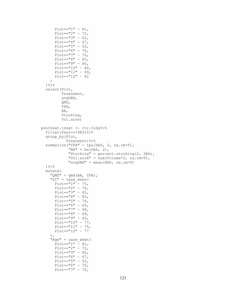
121
Plot=="1" ~ 81,
Plot=="2" ~ 72,
Plot=="3" ~ 62,
Plot=="4" ~ 67,
Plot=="5" ~ 52,
Plot=="6" ~ 70,
Plot=="7" ~ 70,
Plot=="8" ~ 65,
Plot=="9" ~ 80,
Plot=="10" ~ 82,
Plot=="11" ~ 99,
Plot=="12" ~ 82
)
)%>%
select(Plot,
Treatment,
avgDBH,
QMD,
TPA,
BA,
Stocking,
Vol.acre)
pretreat.treat <- ctr.tidy%>%
filter(Year==1983)%>%
group_by(Plot,
Treatment)%>%
summarize("TPA" = tpa(Dbh, 2, na.rm=T),
"BA" = ba(Dbh, 2),
"Stocking" = percent.stocking(2, Dbh),
"Vol.acre" = sum(Volume*2, na.rm=T),
"avgDBH" = mean(Dbh, na.rm=T)
)%>%
mutate(
"QMD" = qmd(BA, TPA),
"SI" = case_when(
Plot=="1" ~ 75,
Plot=="2" ~ 76,
Plot=="3" ~ 65,
Plot=="4" ~ 83,
Plot=="5" ~ 74,
Plot=="6" ~ 69,
Plot=="7" ~ 68,
Plot=="8" ~ 69,
Plot=="9" ~ 69,
Plot=="10" ~ 77,
Plot=="11" ~ 75,
Plot=="12" ~ 77
),
"Age" = case_when(
Plot=="1" ~ 81,
Plot=="2" ~ 72,
Plot=="3" ~ 62,
Plot=="4" ~ 67,
Plot=="5" ~ 52,
Plot=="6" ~ 70,
Plot=="7" ~ 70,

122
Plot=="8" ~ 65,
Plot=="9" ~ 80,
Plot=="10" ~ 82,
Plot=="11" ~ 99,
Plot=="12" ~ 82
)
)%>%
ungroup()%>%
select(-Plot)%>%
group_by(Treatment)%>%
summarize_all(c("mean","stderr"))
#Pre-treatment crop-tree summaries
croptrees.pretreatment <- ctr.tidy%>%
filter(Year==1983 & Classification=="crop-tree")%>%
group_by(Plot,
Treatment)%>%
summarize("TPA" = tpa(Dbh, 2, na.rm=T),
"BA" = ba(Dbh, 2),
"Stocking" = percent.stocking(2, Dbh),
"Vol.tree" = (sum(Volume*2, na.rm=T))/(tpa(which(Dbh>=9.6),
2, na.rm=T)),
"Vol.acre" = sum(Volume*2, na.rm=T),
"avgDBH" = mean(Dbh, na.rm=T)
)%>%
mutate(
"QMD" = qmd(BA, TPA)
)%>%
select(Plot,
Treatment,
avgDBH,
QMD,
TPA,
BA,
Stocking,
Vol.tree,
Vol.acre)
# Removed trees####
#Removed trees 1983
removed.plots <- ctr.tidy%>% #by plot
filter(Year==1983 & Classification=="removed")%>%
group_by(Plot,
Treatment)%>%
summarize("TPA" = tpa(Dbh, 2, na.rm=T),
"BA" = ba(Dbh, 2),
"Vol.acre" = sum(Volume*2, na.rm=T),
"avgDBH" = mean(Dbh, na.rm=T)
)%>%
mutate(
"QMD" = qmd(BA, TPA)
)%>%
select(Plot,
Treatment,
avgDBH,
QMD,

123
TPA,
BA,
Vol.acre)
removed.treat <- ctr.tidy%>% #by treatment
filter(Year==1983 & Classification=="removed")%>%
group_by(Plot,
Treatment)%>%
summarize("TPA" = tpa(Dbh, 2, na.rm=T),
"BA" = ba(Dbh, 2),
"Vol.acre" = sum(Volume*2, na.rm=T),
"avgDBH" = mean(Dbh, na.rm=T)
)%>%
mutate(
"QMD" = qmd(BA, TPA)
)%>%
ungroup()%>%
select(-Plot)%>%
group_by(Treatment)%>%
summarize_all(c("mean", "stderr"))
# Post-treatment ####
posttreat.plots <- ctr.tidy%>% #by plot
filter(Year==1983 & Classification != "removed")%>%
group_by(Plot,
Treatment)%>%
summarize("TPA" = tpa(Dbh, 2, na.rm=T),
"BA" = ba(Dbh, 2),
"Stocking" = percent.stocking(2, Dbh),
"Vol.acre" = sum(Volume*2, na.rm=T),
"avgDBH" = mean(Dbh, na.rm=T)
)%>%
mutate(
"QMD" = qmd(BA,TPA),
"SI" = case_when(
Plot=="1" ~ 75,
Plot=="2" ~ 76,
Plot=="3" ~ 65,
Plot=="4" ~ 83,
Plot=="5" ~ 74,
Plot=="6" ~ 69,
Plot=="7" ~ 68,
Plot=="8" ~ 69,
Plot=="9" ~ 69,
Plot=="10" ~ 77,
Plot=="11" ~ 75,
Plot=="12" ~ 77
),
"Age" = case_when(
Plot=="1" ~ 81,
Plot=="2" ~ 72,
Plot=="3" ~ 62,
Plot=="4" ~ 67,
Plot=="5" ~ 52,
Plot=="6" ~ 70,

124
Plot=="7" ~ 70,
Plot=="8" ~ 65,
Plot=="9" ~ 80,
Plot=="10" ~ 82,
Plot=="11" ~ 99,
Plot=="12" ~ 82
)
)%>%
select(Plot,
Treatment,
avgDBH,
QMD,
TPA,
BA,
Stocking,
Vol.acre)
posttreat.treat <- ctr.tidy%>%
filter(Year==1983 & Classification != "removed")%>%
group_by(Plot,
Treatment)%>%
summarize("TPA" = tpa(Dbh, 2, na.rm=T),
"BA" = ba(Dbh, 2),
"Stocking" = percent.stocking(2, Dbh),
"Vol.acre" = sum(Volume*2, na.rm=T),
"avgDBH" = mean(Dbh, na.rm=T)
)%>%
mutate(
"QMD" = qmd(BA, TPA),
"SI" = case_when(
Plot=="1" ~ 75,
Plot=="2" ~ 76,
Plot=="3" ~ 65,
Plot=="4" ~ 83,
Plot=="5" ~ 74,
Plot=="6" ~ 69,
Plot=="7" ~ 68,
Plot=="8" ~ 69,
Plot=="9" ~ 69,
Plot=="10" ~ 77,
Plot=="11" ~ 75,
Plot=="12" ~ 77
),
"Age" = case_when(
Plot=="1" ~ 81,
Plot=="2" ~ 72,
Plot=="3" ~ 62,
Plot=="4" ~ 67,
Plot=="5" ~ 52,
Plot=="6" ~ 70,
Plot=="7" ~ 70,
Plot=="8" ~ 65,
Plot=="9" ~ 80,
Plot=="10" ~ 82,
Plot=="11" ~ 99,
Plot=="12" ~ 82
)

125
)%>%
ungroup()%>%
select(-Plot)%>%
group_by(Treatment)%>%
summarize_all(c("mean","stderr"))
# Appendix B: Plots ####
# Plot summaries ####
plotsums <- ctr.tidy %>%
mutate(Year = as.numeric(Year))%>%
filter(Classification != "removed" | Year != 1983) %>%
group_by(Plot,
Treatment,
Year) %>%
summarize("TPA" = tpa(Dbh, 2, na.rm=T),
"BA" = ba(Dbh, 2),
"Stocking" = percent.stocking(2, Dbh),
"Volume.tree" = (sum(Volume*2,
na.rm=T))/(tpa(which(Dbh>=9.6), 2, na.rm=T)),
"Volume.acre" = sum(Volume*2, na.rm=T),
"dbh" = mean(Dbh, na.rm=T),
"Ingrowth" = (2*length(which(Ingrowth==1))), #per acre
"Mortality" = (2*length(which(Mortality==T))) #per acre
)%>%
mutate(
"qmd" = qmd(BA, TPA),
"Ingrowth" = cumsum(Ingrowth),
"Total_Mortality" = cumsum(Mortality)
)%>%
left_join(SI.AGE)%>%
select("Plot",
"Treatment",
"Year",
"Age",
"SI",
"Ingrowth",
"TPA",
"Mortality",
"Total_Mortality",
"qmd",
"dbh",
"BA",
"Stocking",
"Volume.tree",
"Volume.acre")
#Take the mean and standard error of plot summaries
treatsums <- plotsums%>%
ungroup()%>%
select(-Plot)%>%
group_by(Treatment,
Year) %>%
summarize_all(
list(Mean = mean, SE = stderr)
)

126
#Summary statistics
#use pivot_longer to create a table with each Variable in one column
#and the corresponding value in another column ("x")
#then group_by treatment, year, and variable
#and summarize using typical summary stats
summarystats <- plotsums %>%
pivot_longer(c(4:15), names_to = "Variable", values_to = "x") %>%
group_by(
Treatment, Year, Variable
) %>%
summarize(
Number = length(x),
Min = min(x),
First_Quartile = quantile(x, 0.25),
Median = median(x),
Third_Quartile = quantile(x, 0.75),
Max = max(x),
Mean = mean(x),
St.Dev = sd(x)
)
#write summary stats as a .csv file
write_csv(summarystats, "summary_stats.csv")
#Create plots over time for all trees
#remove standard error in order to iterate over dataset
treatmeans <- treatsums%>%
select(Treatment,
Year,
ends_with("Mean"))%>%
ungroup()%>%
select(
"Treatment",
"Year",
"Ingrowth" = "Ingrowth_Mean",
"TPA" = "TPA_Mean",
"Mortality" = "Mortality_Mean",
"Total_Mortality" = "Total_Mortality_Mean",
"qmd" = "qmd_Mean",
"dbh" = "dbh_Mean",
"BA" = "BA_Mean",
"Percent_Stocking" = "Stocking_Mean",
"Volume_per_tree" = "Volume.tree_Mean",
"Volume_per_acre" = "Volume.acre_Mean"
)%>%
mutate(
Treatment = as.factor(Treatment)
)
#write chart function
ctrcharts = function(x,y) {
ggplot(treatmeans, aes_string(x=x, y = y,
color=treatmeans$Treatment)) +

127
scale_color_manual(values=c("Control"="black", "20_CTR"="blue",
"34_CTR"="red")) +
geom_point() +
geom_line() +
labs(x=x,
y=y
) +
theme_classic()
}
#set names of response variables
response = names(treatmeans)
response = set_names(response)
#use map function to iterate over each variable in "treatmeans"
ctr_charts <-
map(response,
~map("Year", ctrcharts, y = .x))
#set names for charts
chartnames <- imap(ctr_charts, ~paste0(.y, "", names(.x), ".png")) %>%
flatten()
#save files
walk2(chartnames, flatten(ctr_charts), ~ggsave(filename = .x, plot =
.y,
height = 7, width = 7))
# Crop-tree summaries ####
croptrees.tidy <- ctr.tidy%>%
filter(Classification == "crop-tree")%>%
filter(Plot != 1 | ID != 154,
Plot != 1 | ID != 40,
Plot != 3 | ID != 145,
Plot != 4 | ID != 15,
Plot != 5 | ID != 177,
Plot != 6 | ID != 304,
Plot != 6 | ID != 39,
Plot != 6 | ID != 199,
Plot != 7 | ID != 227,
Plot != 7 | ID != 117,
Plot != 8 | ID != 112,
Plot != 9 | ID != 29,
Plot != 9 | ID != 89,
Plot != 10 | ID != 256,
Plot != 11 | ID != 240,
Plot != 11 | ID != 111,
Plot != 11 | ID != 146,
Plot != 12 | ID != 86,
Plot != 12 | ID != 147,
Plot != 12 | ID != 136,
Plot != 12 | ID != 47,
Plot != 12 | ID != 38
) # filter out crop-trees that died
plotsums.ct <- croptrees.tidy %>%
group_by(Plot,

128
Treatment,
Year) %>%
summarize("TPA" = tpa(Dbh, 2, na.rm=T),
"BA" = ba(Dbh, 2),
"Stocking" = percent.stocking(2, Dbh),
"Volume.tree" = (sum(Volume*2,
na.rm=T))/(tpa(which(Dbh>=9.6), 2, na.rm=T)),
"Volume.acre" = sum(Volume*2, na.rm=T),
"dbh" = mean(Dbh, na.rm=T)
)%>%
mutate(
"qmd" = qmd(BA,TPA))%>%
select("Plot",
"Treatment",
"Year",
"qmd",
"dbh",
"BA",
"Stocking",
"Volume.tree",
"Volume.acre")
#Take the mean and standard error of plot summaries
treatsums.ct <- plotsums.ct%>%
ungroup()%>%
select(-Plot)%>%
group_by(Treatment,
Year) %>%
summarize_all(
list(Mean = mean, SE = stderr)
)
summarystats.ct<-plotsums.ct %>%
pivot_longer(c(4:9), names_to = "Variable", values_to = "x")%>%
group_by(
Treatment, Year, Variable
) %>%
summarize(
Number = length(x),
Min = min(x),
First_Quartile = quantile(x, 0.25),
Median = median(x),
Third_Quartile = quantile(x, 0.75),
Max = max(x),
Mean = mean(x),
St.Dev = sd(x)
)
#write .csv
write_csv(summarystats.ct, "croptrees_summarystats.csv")
#Line Charts
treatmeans.ct <- treatsums.ct%>%

129
select(Treatment,
Year,
ends_with("Mean"))%>%
ungroup()%>%
select(
"Treatment",
"Year",
"qmd" = "qmd_Mean",
"dbh" = "dbh_Mean",
"BA" = "BA_Mean",
"Percent_Stocking" = "Stocking_Mean",
"Volume_per_tree" = "Volume.tree_Mean",
"Volume_per_acre" = "Volume.acre_Mean"
)%>%
mutate(
Treatment = as.factor(Treatment),
Year = as.numeric(Year)
)
#write chart function
linecharts = function(x,y) {
ggplot(treatmeans.ct, aes_string(x=x, y = y,
color=treatmeans.ct$Treatment)) +
scale_color_manual(values=c("Control"="black", "20_CTR"="blue",
"34_CTR"="red")) +
geom_point() +
geom_line() +
labs(x=x,
y=y) +
theme_classic()
}
#set names of response variables
response = names(treatmeans.ct)
response = set_names(response)
line_charts <-
map(response,
~map("Year", linecharts, y = .x))
#set names for charts
chartnames <- imap(line_charts, ~paste0(.y, "", names(.x),
"_croptree.png")) %>%
flatten()
#save files
walk2(chartnames, flatten(line_charts), ~ggsave(filename = .x, plot =
.y,
height = 7, width = 7))

130
REFERENCES
Abrams, M.D. 1990. Adaptations and responses to drought in Quercus species of North
America. Tree Physiology 7:227-238.
Abrams, M.D. 2003. Where has all the white oak gone? BioScience 53(10):927-939.
Abrams, M.D., and G.J. Nowacki. 1992. Historical variation in fire, oak recruitment, and
post-logging accelerated succession in central Pennsylvania. Bulletin of the Torrey
Botanical Club 119(1):19-28.
Beck, D.E. 1987. Management options for southern Appalachian hardwoods: the two-aged
stand. P. 451-454 in Proceedings of the Fourth biennial southern silvicultural
research conference. 1996 November 4-6; Atlanta, GA. General Technical Report
SE-42. Asheville, NC: US Department of Agriculture, Forest Service, Southeastern
Forest Experiment Station.
Brooke, J.M, P.S. Basinger, J.L. Birckhead, M.A. Lashley, J.M. McCord, J.S. Nanney, and
C.A. Harper. 2019. Effects of fertilization and crown release on white oak (Quercus
alba) masting and acorn quality. Forest Ecology and Management 433:305-312.
Brzostek, E.R., D. Dragoni, H.P. Schmid, A.F. Rahman, D. Sims, C.A. Wayson, D.J.
Johnson, and R.P. Phillips. 2014. Chronic water stress reduces tree growth and the
carbon sink of deciduous hardwood forests. Global change biology 20(8):2531-2539.
Butler, B.J. 2008. Family forest owners of the United States, 2006.
Cho D.S., and R.E.J. Boerner. 1991. Canopy disturbance patterns and regneration of Quercus
species in two Ohio old-growth forests. Vegetatio 93:9-18.
Cleland, D.T., J.A. Freeouf, J.E. Keys, G.J. Nowacki, C.A. Carpenter, and W.H. McNab.
2007. Ecological Subregions: Sections and Subsections for the conterminous United
States.
131
Clotfelter, E.D., A.B. Pedersen, J.A. Cranford, N. Ram, E.A. Snajdr, V. Nolan, and E.D.
Ketterson. 2007. Acorn mast drives long-term dynamics of rodent and songbird
populations. Oecologia 154(3):493-503.
Dai, A. 2019. The Climate Data Guide: Palmer Drought Severity Index (PDSI). National
Center For Atmospheric Research Staff (ed.),
https://climatedataguide.ucar.edu/climate-data/palmer-drought-severity-index-pdsi.
Dale, M.E. 1968. Growth response from thinning young even-aged white oak stands. P. 19.
U.S. Department of Agriculture, Forest Service, Northeastern Forest Experiment
Station, Upper Darby, PA.
Demchik, M.C., J.L. Conrad IV, M.M. Vokoun, B. Backes, I. Schellhaass, and B.M.
Demchik. 2018. Crop tree release guidelines for 71-to 94-year-old oak stands based
on height and financial maturity. Journal of Forestry 116(3):217-221.
Dey, D.C. 2014. Sustaining oak forests in eastern North America: regeneration and
recruitment, the pillars of sustainability. Forest Science 60(5):926-942.
Dey, D.C., and R.P. Guyette. 2000. Sustaining Oak Ecosystems in the Central Hardwood
Region: Lessons from the Past--Continuing the History of Disturbance. in Trans.
65th No. Amer. Wildl. and Natur. Resour. Conf. p. 170-183.
Dey, D.C., A.A. Royo, P.H. Brose, T.F. Hutchinson, M.A. Spetich, and S.H. Stoleson. 2010.
An ecologically based approach to oak silviculture: a synthesis of 50 years of oak
ecosystem research in North America. Colombia Forestal 13(2):201-222
Fox, J., and S. Weisberg. 2011. An R companion to applied regression. Sage, Thousand Oaks, CA.
Gauthier, M., and D.F. Jacobs. 2018. Ecophysiological drivers of hardwood plantation
diameter growth under non-limiting light conditions. Forest Ecology and
Management 419:220-226.

132
Gingrich, S.F. 1967. Measuring and evaluating stocking and stand density in upland
hardwood forests in the Central States. Forest Science 13(1):38-53.
Graney, D.L. 1998. Ten-year growth response of red and white oak crop trees to intensity of
crown release. P. 163-168 in Proceedings of the ninth biennial southern silvicultural
research conference. General Technical Repprt SRS-20. Asheville, NC: US
Department of Agriculture, Forest Service, Southern Research Station.
Grunwald, N.J., M. Garbelotto, E.M. Goss, K. Huengens, and S. Prospero. 2012.
Emergence of the sudden oak death pathogen Phytophthora ramorum. Trends in
Microbiology 20(3):131-138.
Hanks, L.F. 1976. Hardwood tree grades for factory lumber. Upper Darby, Pa.: U.S. Dept.
of Agriculture, Forest Service, Northeastern Forest Experiment Station.
Hatcher, J.E., T.J. Straka, and J.L. Greene. 2013. The size of forest holding/parcelization
problem in forestry: A literature review. Resources 2(2):39-57.
Herbohn, J. 2006. Small-scale forestry: is it simply a smaller version of industrial (large-scale)
multiple use forestry. P. 158-163 in Small-scale forestry and rural development: the
intersection of ecosystems, economics and society. Proceedings of IUFRO 3.08
Conference, hosted by Galway-Mayo Institute of Technology, Galway, Ireland.
Holley, A., J.R. Brooks, and S.A. Moss. 2014. Converting international ¼ inch tree volume
to Doyle. P. 295-298 in Proceedings, 19th Central Hardwood Forest Conference;
2014 March 10-12; Carbondale, IL. General Technical Report NRS-P-142. Newtown
Square, PA: US Department of Agriculture, Forest Service, Northern Research
Station: 295-298.
Kenefic, L.S., M. Bataineh, J.S. Wilson, J.C. Brissette, and R.D. Nyland. 2014. Silvicultural
rehabilitation of cutover mixedwood stands. Journal of Forestry 112(3):261-271.

133
Kentucky Division of Forestry. 2010. Kentucky Statewide Assessment of Forest Resources
and Strategy.
Keyser, Chad E., comp. 2008 (revised October 2, 2019). P. 82. Southern (SN) Variant
Overview: Forest Vegetation Simulator. Fort Collins, CO: US Department of
Agriculture, Forest Service, Forest Management Service Center.
Lamson, N.I. 1989. Crop-tree release increases growth of 12-year-old yellow-poplar and
black cherry. US Department of Agriculture, Forest Service, Northeastern Forest
Experiment Station.
Lamson, N.I., and H.C. Smith. 1978. Response to crop-tree release: sugar maple, red oak,
black cherry, and yellow-poplar saplings in a 9-year-old stand. Department of
Agriculture, Forest Service, Northeastern Forest Experiment Station.
Lamson, N.I., H.C. Smith, A.W. Perkey, and S.M. Brock. 1990. Crown release increases
growth of crop trees. Res. Pap. NE-635. Radnor, PA: US Department of Agriculture,
Forest Service, Northeastern Forest Experiment Station. 8 p. 635.
Laws, J. 2018. Investment appraisal. P. 87-106 in Essentials of Financial Management.
Liverpool University Press.
Lenth, R. 2018. emmeans: Estimated marginal means, aka least-squares means. R package version 1.3.0.
Lhotka, J.M., D.L. Parrott, and C.M. Ruffner. 2016. A Dendroecological Investigation of an
Upland Oak-Dominated Forest within the Grand Prairie Region of Illinois. Natural
areas journal 36(3):310-322.
Lovett, G.M., C.D. Canham, M.A. Arthur, K.C. Weathers, and R.D. Fitzhugh. 2006. Forest
Ecosystem Responses to Exotic Pests and Pathogens in Eastern North America.
BioScience 56(5):395-405.

134
McNab, W.H. 2010. Stand response of 16-year-old upland hardwood regeneration to crop-
tree release on a medium quality site in the Southern Appalachians after 24 years.
Res. Note SRS-18. Asheville, NC: US Department of Agriculture, Forest Service,
Southeastern Forest Experiment Station. 2 p. 18.
Meadows, J.S. 1998. Growth and epicormic branching of residual trees following deferment
cutting in red oak-sweetgum stands. P. 148-153 in Proceedings of the ninth biennial
southern silvicultural research conference. General Technical Report SRS-20.
Asheville, NC: US Department of Agriculture, Forest Service, Southern Research
Station.
Mehmood, S.R., and D. Zhang. 2001. Forest parcelization in the United States: a study of
contributing factors. Journal of Forestry 99(4):30-34.
Mesavage, C., and J.W. Girard. 1946. Tables for estimating board-foot volume of timber. P.
94, US Department of Agriculture, Forest Service, Washington, DC.
Miller, G.W. 1984. Releasing young hardwood crop trees: Use of a chain saw costs less than
herbicides. US Department of Agriculture, Forest Service, Northeastern Forest
Experiment Station.
Miller, G.W. 1996. Epicormic branching on central Appalachian hardwoods 10 years after
deferment cutting. US Department of Agriculture, Forest Service, Northeastern
Forest Experiment Station.
Miller, G.W. 2000. Effect of crown growing space on the development of young hardwood
crop trees. Northern Journal of Applied Forestry 17(1):25-35.
Miller G.W., and J.W. Stringer. 2004. Effect of crown release on tree grade and DBH growth
of white oak sawtimber in Eastern Kentucky. P. 37-44 in Proceedings, 14th Central
Hardwood Forest Conference. 2004 March 16-19; Wooster, OH. General Technical

135
Report NE-316. Newtown Square, PA: US Department of Agriculture, Forest
Service, Northeastern Research Station.
Miller, G.W., L.F. Hanks, and H.V. Wiant, Jr. 1986. A key for the Forest Service hardwood
tree grades. Northern journal of applied forestry(1):19-22.
Morrissey, R., M. Saunders, and W. Hoover. 2011. Financial and Wildlife Benefits from Crop
Tree Release in Pole-Sized Central Hardwood Oak Stands. Northern Journal of
Applied Forestry 28(1):5-12.
Nadkarni, N.M., P.H. Hasbach, T. Thys, E.G. Crockett, and L. Schnacker. 2017. Impacts of
nature imagery on people in severely nature‐deprived environments. Frontiers in
Ecology and the Environment 15(7):395-403.
Nowacki G.J., M.D. Abrams, and C.G. Lorimer. 1990. Composition, structure, and historical
development of northern red oak stands along an edaphic gradient in north-central
Wisconsin. Forest Science 36:276-292.
Oswalt, Oswalt M., and Roger C. Conner. 2011. Southern Forest Inventory and Analysis
Volume Equation User’s Guide. General Techincal Report SRS-138. US Department
of Agriculture, Forest Service. Southern Research Station.
R Core Team 2020. R: A language and environment for statistical computing. R Foundation
for Statistical Computing, Vienna, Austria.
Roach B.A, and S.F. Gingrich. 1968. Even-aged silviculture for upland central hardwoods.
Agriculture Handbook 355. Washington D.C.: US Department of Agriculture, Forest
Service, Northeastern Forest Experiment Station.
Schuler, T.M. 2006. Crop tree release improves competitiveness of northern red oak growing
in association with black cherry. Northern Journal of Applied Forestry 23(2):77-82.

136
Sendak, P.E. 2008. Early crop-tree release and species cleaning in young northern
hardwoods: a financial analysis. US Department of Agriculture, Forest Service,
Northern Research.
Shifley, S.R., Z. Fan, J.M. Kabrick, and R.G. Jensen. 2006. Oak mortality risk factors and
mortality estimation. Forest Ecology and Management 229(1-3):16-26.
Smith, H.C. 1983. Precommercial crop-tree release increases diameter growth of
Appalachian hardwood saplings. US Department of Agriculture, Forest Service,
Northeastern Forest Experiment.
Smith, H.C., G.W. Miller, and N.I. Lamson. 1994. Crop-tree release thinning in 65-year-old
commercial cherry-maple stands (5-year results). US Department of Agriculture,
Forest Service, Northeastern Forest Experiment.
Sonderman, D.L. 1987. Stem-quality changes on young, mixed upland hardwoods after crop-
tree release. RP-NE 597. Broomall, PA: US Department of Agriculture, Forest
Service, Northeastern Forest Experiment Station. 7 p. 597.
Stringer, J.W. 1999. Development of advanced oak regeneration from two-age reserve trees.
P. 291-293 in Proceedings, 12th Central Hardwood Forest Conference. 1999 February
28, March 1-2; Lexington, KY. General Technical Report SRS-24. Asheville, NC: US
Department of Agriculture, Forest Service, Southern Research Station.
Stringer, J.W., G.W. Miller, and R.F. Wittwer. 1988. Applying a crop-tree release in small-
sawtimber white oak stands.
Trimble, G.R. 1971. Early crop-tree release in even-aged stands of Appalachian hardwoods.
Northeastern Forest Experiment Station.

137
Trimble, G.R. 1974. Response to crop-tree release by 7-year-old stems of red maple stump
sprouts and northern red oak advance reproduction. US Department of Agriculture,
Forest Service, Northeastern Forest Experiment.
Ward, J.S. 2002. Crop tree release increases growth of mature red oak sawtimber. Northern
Journal of Applied Forestry 19(4):149-154.
Ward, J.S. 2007. Crop-tree release increases growth of black birch (Betula lenta L.) in
southern New England. Northern Journal of Applied Forestry 24(2):117-122.
Ward, J.S. 2008. Crop tree release increases growth of red oak sawtimber in southern New
England: 12-year results. in 16th Central Hardwood Forest Conference; 2008 April
8-9; West Lafayette, IN. Gen. Tech. Rep. NRS-P-24. Newtown Square, PA: US
Department of Agriculture, Forest Service, Northern Research Station: 457-465.
Ward, J.S. 2009. Intensity of precommercial crop tree release increases diameter growth and
survival of upland oaks. Canadian Journal of Forest Research 39(1):118-130.
Ward, J.S. 2013. Precommercial crop tree release increases upper canopy persistence and
diameter growth of oak saplings. Northern Journal of Applied Forestry 30(4):156-
163.
Ward, J.S. 2017. Twenty-five year response of non-crop trees to partial release during
precommercial crop tree management. Forest Ecology and Management 387:12-18.
West, S. 2019. Kentucky Delivered Log Price Report (3rd. and 4th. Qtrs. 2019).
Wiant, H.V. 1986. Computer Corner. Northern Journal of Applied Forestry 3(3):124-124.

138
VITA
Philip Jay Vogel EDUCATION University of Kentucky, Bachelor of Science in Forestry, 2015 University of Kentucky, Minor in English, 2015 PROFESSIONAL POSITIONS Graduate Research Assistant, University of Kentucky, 2018-2020 Horticulture Crew Foreman, LFUCG, 2017-2018