long-run risks and risk compensation in equity markets
TRANSCRIPT
Els UK ch05-n50899.pdf 2007/9/5 2:56 pm Page: 167 Trim: 7.5in × 9.25in Floats: Top/Bot TS: diacriTech, India
CHAPTER 5
Long-Run Risks and RiskCompensation in Equity Markets
Ravi Bansal∗Fuqua School of Business, Duke University, and NBER
1. Introduction 1682. Long-Run Risks Model 170
2.1. Preferences and the Environment 1702.2. Long-Run Growth Rate Risks 1712.3. Long-Run Growth and Uncertainty Risks 1742.4. Data and Model Implications 176
3. Cross-Sectional Implications 1853.1. Value, Momentum, Size, and the Cross-Sectional Puzzle 185
4. Conclusion 191References 191
Abstract
What drives the compensation in equity markets? This article shows that long-rungrowth and economic uncertainty in the economy play an important role in determiningthe risk in equity markets. The size of the market risk premium, the level of the risk-freerate, the volatility of asset prices, and differences in the risk compensation across assetsare shown to be related to risks pertaining to the long-run growth and uncertainty in theeconomy.
JEL Classification: G12, E44
Keywords: long-run risks, volatility risks, intertemporal elasticity of substitution
∗I thank Amir Yaron, Dana Kiku, John Heaton, and Lars Hansen, and the Editor, Raj Mehra, for theircomments. The usual disclaimer applies.
HANDBOOK OF THE EQUITY RISK PREMIUMCopyright c© 2008 by Elsevier BV. All rights of reproduction in any form reserved. 167

Els UK ch05-n50899.pdf 2007/9/5 2:56 pm Page: 168 Trim: 7.5in × 9.25in Floats: Top/Bot TS: diacriTech, India
168 Chapter 5 • Long-Run Risks and Risk Compensation in Equity Markets
1. INTRODUCTION
Several aspects of asset markets are puzzling. The work of Mehra and Prescott (1985)shows that the magnitude of risk compensation in equity markets is a puzzle—Treasurybills offer a return of about 1 percent per annum while the equity market portfolio offers7.5 percent. What risks justify such a sizable compensation for holding equity? Anotherequally puzzling, and related, dimension is the large difference in the average returnsacross equity portfolios. For example, the return to value firms exceeds that of growthfirms by about 7 percent per annum. In addition to these return puzzles, Shiller (1981)and Leroy and Porter (1981) document the volatility puzzle—it is hard to explain thehigh volatility of equity prices. This article highlights the ideas developed in Bansal andLundblad (2002), Bansal and Yaron (2004), Bansal, Khatchatrian, and Yaron (2005),Bansal, Dittmar, and Lundblad (2002, 2005), and Bansal, Gallant, and Tauchen (2007)pertaining to various financial market anomalies. This research argues that the magni-tudes of asset returns and volatility are a natural outcome of risks associated with thelong-run growth prospects and changing economic uncertainty in the economy.
Bansal and Yaron (2004) argue that investors care about the long-run growthprospects and the level of economic uncertainty. Changes in these fundamentals drivethe risks and volatility in asset prices. They document that consumption and dividendgrowth rates contain a small long-run component. That is, current shocks to expectedgrowth alter expectations about future economic growth not only for short horizons butalso for the very long run. Agents care a lot about these long-run components as smallrevisions in them lead to large changes in asset prices. Any adverse movements in thelong-run growth components lower asset prices and concomitantly the wealth and con-sumption of investors. This makes holding equity very risky for investors, making themdemand a high equity risk compensation.
Bansal and Yaron further argue that time variation in expected excess returns isdue to variation in economic uncertainty. They model this uncertainty by incorporatingtime-varying consumption volatility in the consumption process. Empirical motivationfor this channel is provided by Bansal, Khatchatrian, and Yaron (2005)—their robustempirical finding is that current consumption volatility predicts future asset valuationsand that current asset valuations predict future consumption volatility. Both projec-tion coefficients are significantly negative. A rise in economic uncertainty lowers assetprices—that is, asset markets dislike economic uncertainty. Bansal and Yaron derive theresult that volatility shocks, in equilibrium, carry a separate risk premium; this is a novelfeature of their model.
Epstein and Zin (1989) preferences play an important role in the Bansal and Yaronmodel. These preferences allow for separation between risk aversion and the intertem-poral elasticity of substitution (IES) of investors. An IES larger than one is required forthe wealth to consumption ratio to rise with expected consumption growth; when theIES is smaller than one, high expected growth lowers the wealth to consumption ratio.The equity price to dividend ratio mirrors the behavior of the wealth to consumptionratio. This ensures that equity payoffs are high when consumption and corporate profitsrise, leading to a positive equity risk premium. An IES larger than one is also requiredto capture the data feature that asset markets dislike economic uncertainty.

Els UK ch05-n50899.pdf 2007/9/5 2:56 pm Page: 169 Trim: 7.5in × 9.25in Floats: Top/Bot TS: diacriTech, India
Ravi Bansal 169
The magnitude of the IES is a key empirical issue. Hansen and Singleton (1982),Attanasio and Weber (1989), and Attanasio and Vissing-Jorgensen (2003) estimate theIES to be well in excess of one. Hall (1988) and Campbell (1999), on the other hand,estimate its value to be well below one. Bansal and Yaron argue that the estimates for theIES in Hall and Campbell are not a robust guide for the magnitude of the IES parameter.They show that even if the population value of the IES is larger than one, the estimationmethods used by Hall would measure the IES to be close to zero. That is, there is a severedownward bias in the point estimates of the IES. Bansal and Yaron as well as Bansal,Khatchatrian, and Yaron (2005) further argue that the economic implications when theIES is less than one—a rise in consumption volatility and/or a drop is expected growthraises asset valuations, are counterfactual, making the low magnitude of the IES suspect.
The arguments presented in Bansal and Yaron also have immediate implications forthe cross-sectional differences in mean returns across assets. Firms whose expectedcash-flow (profits) growth rates move with the economy are more exposed to long-run risks and hence should carry a higher risk compensation. In Breeden (1979), Lucas(1978), and Hansen and Singleton (1982), the riskiness of the asset is determined bythe consumption beta of the asset. However, the consumption beta of an asset is notexogenous—in equilibrium, it is determined by the systematic risks in cash flows andthe preference parameters of the representative agent. That is, cross-sectional differ-ences in betas of assets reflect differences in the systematic risks in cash flows. Risks incash flows should consequently contain information about differences in mean returnsacross assets. We review the work of Bansal, Dittmar, and Lundblad (2002, 2005), whoshow that systematic risks in cash flows can account for the cross-sectional differencesin risk premia of assets. Specifically, their cash-flow betas can account for the puzzlingvalue, size, and the momentum spread in the cross section of assets.
Bansal and Lundblad (2002) rely on long-run components and varying riskpremia to address issues in international equity markets. Developed markets’ assetprices and returns show a high degree of correlation; however, dividends and earningsgrowth across these economies are virtually uncorrelated. Bansal and Lundblad showthat high asset price volatility and correlation across national equity markets are due tothe long-run component in dividend growth rates and time-varying systematic risk.
The argument that long-term economic growth and uncertainty are the key driversof risks in equity markets is distinct from the arguments presented in Campbell andCochrane (1999). They argue that equity market risks are driven largely (even exclu-sively) by fluctuations in the ex-ante rate of discount (cost of capital) through externalhabit formation. Sorting out which of the channels is critical for explaining the riskcompensation in equity markets, consequently, is largely an empirical issue. Usingthe Efficient Method of Moments (EMM) estimation technique, Bansal, Gallant, andTauchen (2007) document the differences between the Bansal and Yaron and Campbelland Cochrane models. A unique dimension of the Bansal, Gallant, and Tauchen paper isthat consumption and dividends in their model are cointegrated—this feature is typicallymissing in earlier work on asset market models.
The remainder of the article has three sections. Section 2 discusses the long-run risksmodel of Bansal and Yaron. Section 3 discusses the issue of cross-sectional differencesin returns across asset portfolios. Section 4 presents concluding comments.
Els UK ch05-n50899.pdf 2007/9/5 2:56 pm Page: 170 Trim: 7.5in × 9.25in Floats: Top/Bot TS: diacriTech, India
170 Chapter 5 • Long-Run Risks and Risk Compensation in Equity Markets
2. LONG-RUN RISKS MODEL
2.1. Preferences and the Environment
We consider a representative agent with the generalized preferences developed inEpstein and Zin (1989). The logarithm of the Intertemporal Marginal Rate of Substitu-tion (IMRS), mt+1, for these preferences, as shown in the Epstein and Zin paper, is
mt+1 = θ log δ − θ
ψgt+1 + (θ − 1)ra,t+1. (1)
If Rt+1 is the gross return on the asset, then log (Rt+1) ≡ rt+1 is the continuous return onthe asset. Using the standard asset pricing restriction for any continuous return ri,t+1, itfollows that1
Et
[exp
(θ log δ − θ
ψgt+1 + (θ − 1)ra,t+1 + ri,t+1
)]= 1, (2)
where gt+1 equals log(Ct+1/Ct)—the log growth rate of aggregate consumption. Thereturn, ra,t+1, is the log of the return (i.e., continuous return) on an asset that deliversaggregate consumption as its dividends each time period. The time discount factor isδ and the parameter θ ≡ 1 − γ/(1 − 1/ψ), where γ ≥ 0 is the risk aversion (sensitivity)parameter, and ψ ≥ 0 is the intertemporal elasticity of substitution. The sign of θ isdetermined by the magnitudes of the risk aversion and the elasticity of substitution.2
Note that when θ equals one, the above IMRS and the asset pricing implications collapseto the usual case of power utility considered in Mehra and Prescott (1985).
The return to the aggregate consumption claim, ra,t+1, is not observed in the datawhile the return on the dividend claim corresponds to the observed return on the marketportfolio rm,t+1. The levels of market dividends and consumption are not equal; aggre-gate consumption is much larger than aggregate dividends. The difference is financed bylabor income. In the model, aggregate consumption and aggregate dividends are treatedas two separate processes and the difference between them implicitly defines the agent’slabor income process.
1Note that the standard asset pricing condition in frictionless markets is
Et[exp(mt+1 + rt+1)] = 1,
where the intertemporal marginal rate of substitution is Mt+1 and log(Mt+1) ≡ mt+1. The logarithm of thegross return for an asset equals rt+1.2In particular, if ψ > 1 and γ > 1, then θ will be negative. Note that when θ = 1, that is, γ = (1/ψ), the aboverecursive preferences collapse to the standard case of expected utility. Further, when θ = 1 and in additionγ = 1, we get the standard case of log utility.
Els UK ch05-n50899.pdf 2007/9/5 2:56 pm Page: 171 Trim: 7.5in × 9.25in Floats: Top/Bot TS: diacriTech, India
Ravi Bansal 171
The key ideas of the model are developed and the intuition is provided viaapproximate analytical solutions. However, all the quantitative results reported in thepaper are based on numerical solutions of the model. To derive the approximate analyt-ical solutions for the model, we use the standard first-order Taylor series approximationdeveloped in Campbell and Shiller (1988),3
ra,t+1 = κ0 + κ1zt+1 − zt + gt+1, (3)
where lowercase letters refer to variables in logs, in particular, ra,t+1 = log(Ra,t+1) isthe continuous return on the consumption claim, and zt ≡ log (Pt/Ct) is the log price toconsumption ratio. Analogously, rm,t+1 and zm,t correspond to the continuous return onthe dividend claim and its log price-dividend ratio. As Pt + Ct/Ct is the agent’s wealthto consumption ratio, fluctuations in the price to consumption ratio, consequently, alsocorrespond to movements in the wealth to consumption ratio. Parameters κ0 and κ1 areapproximating constants that both depend only on the average level of z.4
From Eq. (1) it follows that the innovation in the IMRS, mt+1, is driven by theinnovations in gt+1 and ra,t+1. Covariation with the innovation in mt+1 determines therisk premium for any asset. The simpler model specification, with only long-run growthrate risks, is discussed first. The full model that incorporates long-run growth rate andeconomic uncertainty risks is presented after that.
2.2. Long-Run Growth Rate Risks
The agents’ IMRS depends on the endogenous consumption return, ra,t+1. The riskcompensation on all assets depends on this return, which itself is determined by the pro-cess for consumption growth. The dividend process is needed for determining the returnon the market portfolio. To capture long-run risks, consumption and dividend growthrates, gt+1 and gd,t+1, are modeled to contain a small persistent predictable component xt,
xt+1 = ρxt + ϕeσet+1,gt+1 = µ + xt + σηt+1,gd,t+1 = µd + φxt + ϕdσut+1,
et+1, ut+1, ηt+1 ∼ N.i.i.d.(0, 1),
(4)
3Any equity return can be written as
Rt+1 =1 +
Pt+1
Dt+1
PtDt
Dt+1
Dt.
The approximate return expression follows from taking the log of the gross return and then taking a first-orderTaylor series approximation of log
(1 + Pt+1
Dt+1
)around the average value of the log of the price-dividend ratio,
which is referenced as z in Eq. (3). The approximating constants κ0 and κ1 are solely determined by theaverage value of z.4The Campbell–Shiller approximate return follows from using a first-order Taylor series expansion of thecontinuous return. Note that κ1 = exp(z̄)/(1 + exp(z̄)). The value of κ1 is set at 0.997, which is consistentwith the magnitude of z̄ in our sample and with the magnitudes used in Campbell and Shiller (1988).
Els UK ch05-n50899.pdf 2007/9/5 2:56 pm Page: 172 Trim: 7.5in × 9.25in Floats: Top/Bot TS: diacriTech, India
172 Chapter 5 • Long-Run Risks and Risk Compensation in Equity Markets
with the three shocks, et+1, ut+1, and ηt+1, assumed to be mutually independent. Thevolatility of the consumption growth rate innovation is σ. Similarly, the volatility of theinnovation in xt+1 and gd,t+1 is ϕeσ and ϕdσ, respectively.
The parameter ρ determines the persistence of the expected growth rate process.First, note that when ϕe = 0, the processes gt and gd,t+1 are i.i.d. Second, if et+1 = ηt+1,the process for consumption is the ARMA(1,1) used in Campbell (1999), Cecchetti,Lam, and Mark (1993), and Bansal and Lundblad (2002). If, in addition, ϕe = ρ, thenconsumption growth corresponds to an AR(1) process used in Mehra and Prescott(1985).
Two additional parameters, φ > 1 and ϕd > 1, calibrate the overall volatility of div-idends and its correlation with consumption. The parameter φ can be interpreted, asin Abel (1999), as the leverage ratio on expected consumption growth. Alternately,this says that corporate profits, relative to consumption, are more sensitive to chang-ing expected economic growth conditions. That is, any fluctuation in xt leads to largerchanges in expected dividend growth relative to expected consumption growth. Themaintained assumption is that the three innovations are uncorrelated. It is straightfor-ward to allow the three shocks to be correlated; however, to maintain parsimony in thenumber of parameters, they are assumed to be independent. Note that consumption anddividends are not cointegrated in the above specification—Bansal, Gallant, and Tauchen(2007) develop a specification that does allow for cointegration between consumptionand dividends.
Asset prices reflect expectations of future growth rates. To develop some intuitionabout long-run risks, consider the quantity
Et
[ ∞∑j=1
κj
1gt+j
],
with κ1 less than one, this expectation equals κ1xt/(1 − κ1ρ). Even if the variance ofx is tiny, but ρ fairly high, then shocks to x can alter growth rate expectations for thelong run, leading to volatile asset prices. Bansal and Lundblad (2002) and Bansal andYaron (2004) provide empirical support for the existence of this long-run component inobserved growth rates.
2.2.1. Equilibrium and Asset Prices
The consumption and dividend growth rates processes are exogenous in this endowmenteconomy. Further, the IMRS depends on an endogenous return ra,t+1. To characterize theIMRS and the behavior of asset returns, a solution for the log price to consumption ratiozt and the log price-dividend ratio zm,t is needed. The relevant state variable for derivingthe solution for zt and zm,t is the expected growth rate of consumption xt.
Exploiting the Euler equation (2), the approximate solution for the log price-consumption zt has the form zt = A0 + A1xt. An analogous expression holds for
Els UK ch05-n50899.pdf 2007/9/5 2:56 pm Page: 173 Trim: 7.5in × 9.25in Floats: Top/Bot TS: diacriTech, India
Ravi Bansal 173
the log price-dividend ratio zm,t.5 Bansal and Yaron (2004) show that the solutioncoefficients are
A1 =1 − 1
ψ
1 − κ1ρ, A1,m =
φ − 1ψ
1 − κ1,mρ. (5)
It follows that A1 is positive if the IES, ψ , is greater than one. In this case the intertem-poral substitution effect dominates the wealth effect. In response to higher expectedgrowth, agents buy more assets, and consequently the wealth to consumption ratio rises.The level of consumption rises due to a rise in expected growth; however, wealth risesmore than consumption. In the standard power utility model with risk aversion largerthan one, the IES is less than one, and hence A1 is negative—a rise in expected growthpotentially lowers asset valuations. That is, the wealth effect dominates the substitutioneffect.6 Corporate payouts (i.e., dividends), with φ > 1, are more sensitive to long-runrisks (i.e., A1,m > A1), and changes in expected growth rate lead to a larger reaction inthe price of the dividend claim than in the price of the consumption claim.
Equation (3), the solution in (5), and the dynamics for the consumption and dividendgrowth rates provide a complete characterization for the endogenous returns on theconsumption and the dividend asset.
2.2.2. Pricing of Long-Run Growth Risks
Substituting the equilibrium return for ra,t+1 into the IMRS, Bansal and Yaron show thatthe innovation in mt+1 is
mt+1 − Et(mt+1) = −[ θψ
− θ + 1]σηt+1 − (1 − θ)
[κ1
(1 − 1
ψ
)ϕe
1 − κ1ρ
]σet+1
= −λm,ησηt+1 − λm,eσet+1. (6)
The parameters λm,e and λm,η determine the risk compensation for expected growth rateshock and the independent consumption shock ηt+1.
The risk compensation for the ηt+1 shocks is very standard as λm,η equals the riskaversion parameter γ.7 In addition, with power utility, that is, when θ equals one,λm,e = 0. Long-run risks are priced only when θ differs from one, that is, when riskaversion is not the reciprocal of the IES—this highlights the importance of the gen-eralized preferences of Epstein and Zin (1989). The market price of long-run risks issensitive to the magnitude of the permanence parameter ρ. The risk compensation for
5The expression for the intercept terms A0 for the valuation ratio for the consumption claim, and A0,m for thedividend claim are not important for our qualitative results.6An alternative interpretation with the power utility model is that higher expected growth rates increase therisk-free rate to an extent that discounting dominates the effects of higher expected growth rates. This leadsto a fall in asset prices.7This follows by substituting the expression for θ and simplifying the expression [θ/ψ − θ + 1].

Els UK ch05-n50899.pdf 2007/9/5 2:56 pm Page: 174 Trim: 7.5in × 9.25in Floats: Top/Bot TS: diacriTech, India
174 Chapter 5 • Long-Run Risks and Risk Compensation in Equity Markets
long-run risks, λm,e, rises as the permanence parameter ρ rises. The conditional volatilityof the pricing kernel is constant, as all risk sources have constant conditional variances.
As asset returns and the pricing kernel in this model economy are conditionallylog-normal, the risk premium on any asset i is Et[ri,t+1 − rf ,t] = −covt(mt+1, ri,t+1) −0.5σ2
ri,t. Given the solutions for A1 and A1,m, it is straightforward to derive the equitypremium on the market portfolio,
E(rm,t+1 − rf ,t) = βm,ηλm,ησ2 + βm,eλm,eσ
2 − 0.5Var(rm,t). (7)
The market portfolio’s beta with respect to the long-run risk component is
βm,e ≡[κ1,m
(φ − 1
ψ
)ϕe
1 − κ1,mρ
]. (8)
The exposure of the market return to long-run risk is βm,e, and the market price of thelong-run risk is λm,e. The expressions for these variables reveal that a rise in ρ increasesboth βm,e and λm,e. Consequently, the risk premium on the asset also increases with ρ.The market portfolio’s beta with respect to the short-run risk component ηt+1 is deter-mined by the exposure of the dividend’s innovation to ηt+1. The assumption that thedividend innovation of the market portfolio is independent of the short-run shock inconsumption ηt+1 implies that βm,η will be zero in our calibration exercise.
As all shocks have a constant conditional variance, the conditional risk premium onthe market portfolio and its conditional volatility are constant. The ratio of the two,namely the Sharpe ratio, is also constant. In order to address issues that pertain to time-varying risk premia and predictability of risk premia, Bansal and Yaron augment theabove model by incorporating time-varying economic uncertainty.
2.3. Long-Run Growth and Uncertainty Risks
Bansal and Yaron model fluctuating economic uncertainty as time-varying volatilityof consumption growth. The consumption and dividends dynamics that incorporatestochastic volatility are
xt+1 = ρxt + ϕeσtet+1,
gt+1 = µ + xt + σtηt+1,
gd,t+1 = µd + φxt + ϕdσtut+1, (9)
σ2t+1 = σ2 + ν1(σ2
t − σ2) + σwwt+1,
et+1, ut+1, ηt+1,wt+1 ∼ N.i.i.d.(0, 1),
where σt+1, the conditional volatility of consumption growth, represents the time-varying economic uncertainty incorporated in consumption growth rate. The uncon-ditional mean of the time-varying variance of consumption growth is σ2, andσw determines the volatility of shocks to consumption uncertainty. The parameter ν1
determines the persistence of shocks to consumption variance. To maintain parsimony,it is assumed that the shocks are uncorrelated and only one source of time-varyingeconomic uncertainty affects consumption and dividends.
Els UK ch05-n50899.pdf 2007/9/5 2:56 pm Page: 175 Trim: 7.5in × 9.25in Floats: Top/Bot TS: diacriTech, India
Ravi Bansal 175
The relevant state variables in solving for the equilibrium price-consumption (andprice-dividend) ratio are now xt and σ2
t . Thus, the approximate solution for theprice-consumption ratio is zt = A0 + A1xt + A2σ
2t . The solution for A1 is unchanged
(Eq. (5)). The solution coefficient A2 for measuring the sensitivity of the price-consumption ratio to volatility fluctuations is
A2 =
0.5[(θ − θ
ψ
)2+ (θA1κ1ϕe)2
]
θ(1 − κ1ν1). (10)
An analogous coefficient for the market price-dividend ratio, A2,m, is provided in Bansaland Yaron (2004).
The expression for A2 provides two valuable insights. First, if the IES and risk aver-sion are larger than one, then θ and consequently A2 are negative. In this case, a risein consumption volatility lowers asset valuations and increases the risk premia on allassets. To capture the intuition that a rise in economic uncertainty lowers asset valua-tions requires that the IES be larger than one. Bansal, Khatchatrian, and Yaron (2005)present robust empirical evidence that asset markets dislike economic uncertainty—thatis,A2 is negative. This empirical evidence, given the expression forA2, has a direct bear-ing on the plausible magnitude for the IES. Second, an increase in the permanence ofvolatility shocks, that is ν1, magnifies the effects of volatility shocks on valuation ratiosas changes in economic uncertainty are perceived by investors as being long-lasting.
2.3.1. Pricing of Uncertainty Risks
As the wealth to consumption ratio is affected by consumption volatility shocks, so arethe return ra,t+1 and the IMRS. Specifically, the innovation in mt+1 is
mt+1 − Et(mt+1) = −λm,ησtηt+1 − λm,eσtet+1 − λm,wσwwt+1, (11)
where λm,η, λm,e, and λm,w are the market prices of risks for the short-run, long-run,and volatility risks. The market prices of systematic risks, including the compensationfor stochastic volatility risk in consumption, can be expressed in terms of underlyingpreferences and parameters that govern the evolution of consumption growth as
λm,η = γ,
λm,e =
(γ − 1
ψ
)[ κ1ϕe1 − κ1ρ
], (12)
λm,w =
(γ − 1
ψ
)(1 − γ)
[κ1(1 + ( κ1ϕe1−κ1ρ
)2)
2 (1 − κ1ν1)
].
Expression (11) is similar to the earlier model (see Eq. (6)) save for the inclusion ofwt+1, the shocks to consumption volatility. In the special case of power utility, when
Els UK ch05-n50899.pdf 2007/9/5 2:56 pm Page: 176 Trim: 7.5in × 9.25in Floats: Top/Bot TS: diacriTech, India
176 Chapter 5 • Long-Run Risks and Risk Compensation in Equity Markets
θ = 1 or more specifically, where γ = 1/ψ , the risk compensation parameters λm,e andλm,w are zero. The long-run risks and volatility risks are not reflected in the innovationof the pricing kernel. With power utility there is no separate risk compensation for long-run growth rate risks and volatility risks—with Epstein and Zin preferences, both risksare priced. The pricing of long-run and volatility risks is an important and novel featureof the Bansal and Yaron model.
The equity premium in the presence of time-varying economic uncertainty is
Et(rm,t+1 − rf ,t) = βm,ηλm,ησ2t + βm,eλm,eσ
2t + βm,wλm,wσ
2w − 0.5Vart(rm,t+1), (13)
where βm,w ≡ κ1,mA2,m. The first β corresponds to the exposure to short-run risks, andthe second to long-run risks. The last beta, βm,w , is the exposure of the asset to volatilityrisks.
The risk premium on the market portfolio is time-varying as σt fluctuates. The ratioof the conditional risk premium to the conditional volatility of the market portfoliofluctuates with σt, and hence the Sharpe ratio is time-varying. The maximal Sharperatio in this model economy, which approximately equals the conditional volatility ofthe log IMRS, also varies with σt.8 This implies that during periods of high economicuncertainty all risk premia will rise.
The first-order effects on the level of the risk-free rate, as discussed in Bansal andYaron (2006), are the rate of time preference and the average consumption growth rate,divided by the IES. Increasing the IES keeps the level low. The variance of the risk-freerate is determined by the volatility of the expected consumption growth rate and the IES.Increasing the IES lowers the volatility of the risk-free rate. In addition, incorporatingeconomic uncertainty leads to an interesting channel for interpreting fluctuations in thereal risk-free rate. In particular, Bansal and Yaron show that this has serious implicationsfor the measurement of the IES in the data. In the presence of varying volatility, theestimates of the IES based on the projections considered in Hall (1988) and Campbell(1999) are seriously biased downwards.
2.4. Data and Model Implications
2.4.1. Data and the Growth Rate Dynamics
Bansal and Yaron (2004) calibrate the model described in (4) and (9) at the monthlyfrequency. From this monthly model they derive time-aggregated annual growth ratesof consumption and dividends to match key aspects of annual aggregate consumptionand dividends data. Further, as in Campbell and Cochrane (1999) and in Kandel andStambaugh (1991), they assume that the decision interval of the agent is monthly, butthe targeted data to match is annual.9
8Given the conditional normality of the logarithm of the IMRS, the maximal Sharpe ratio is simply theconditional standard deviation of the logarithm of the IMRS.9The evidence regarding the model is based on numerical solutions using standard polynomial-based projec-tion methods discussed in Judd (1998). The numerical results are quite close to those based on the approximateanalytical solutions.
Els UK ch05-n50899.pdf 2007/9/5 2:56 pm Page: 177 Trim: 7.5in × 9.25in Floats: Top/Bot TS: diacriTech, India
Ravi Bansal 177
For consumption, BEA data on real per capita annual consumption growth ofnon-durables and services for the period 1929–1998 is utilized. This is the longest singledata source of consumption data. Dividends and the value-weighted market return dataare taken from the CRSP. All nominal quantities are deflated using the CPI. To facilitatecomparisons between the model, which is calibrated to a monthly decision interval, andthe annual data, the monthly model is time-aggregated to the annual frequency to deriveannual statistics.
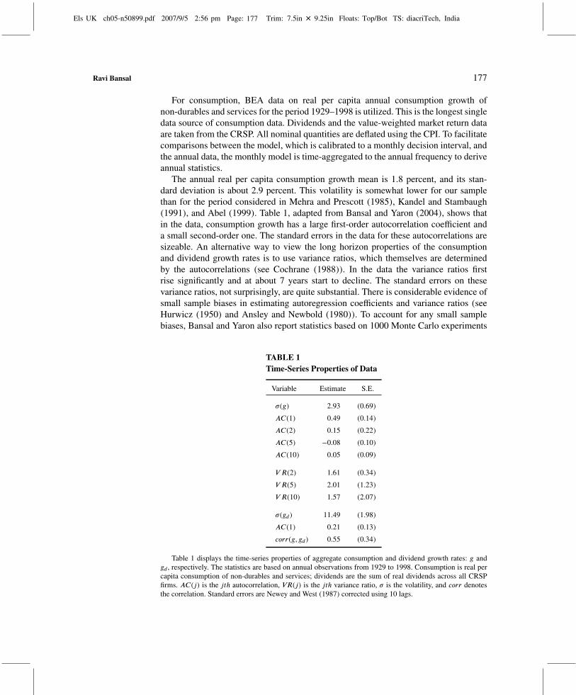
The annual real per capita consumption growth mean is 1.8 percent, and its stan-dard deviation is about 2.9 percent. This volatility is somewhat lower for our samplethan for the period considered in Mehra and Prescott (1985), Kandel and Stambaugh(1991), and Abel (1999). Table 1, adapted from Bansal and Yaron (2004), shows thatin the data, consumption growth has a large first-order autocorrelation coefficient anda small second-order one. The standard errors in the data for these autocorrelations aresizeable. An alternative way to view the long horizon properties of the consumptionand dividend growth rates is to use variance ratios, which themselves are determinedby the autocorrelations (see Cochrane (1988)). In the data the variance ratios firstrise significantly and at about 7 years start to decline. The standard errors on thesevariance ratios, not surprisingly, are quite substantial. There is considerable evidence ofsmall sample biases in estimating autoregression coefficients and variance ratios (seeHurwicz (1950) and Ansley and Newbold (1980)). To account for any small samplebiases, Bansal and Yaron also report statistics based on 1000 Monte Carlo experiments
TABLE 1Time-Series Properties of Data
Variable Estimate S.E.
σ(g) 2.93 (0.69)
AC(1) 0.49 (0.14)
AC(2) 0.15 (0.22)
AC(5) −0.08 (0.10)
AC(10) 0.05 (0.09)
V R(2) 1.61 (0.34)
V R(5) 2.01 (1.23)
V R(10) 1.57 (2.07)
σ(gd) 11.49 (1.98)
AC(1) 0.21 (0.13)
corr(g, gd) 0.55 (0.34)
Table 1 displays the time-series properties of aggregate consumption and dividend growth rates: g andgd, respectively. The statistics are based on annual observations from 1929 to 1998. Consumption is real percapita consumption of non-durables and services; dividends are the sum of real dividends across all CRSPfirms. AC(j) is the jth autocorrelation, VR(j) is the jth variance ratio, σ is the volatility, and corr denotesthe correlation. Standard errors are Newey and West (1987) corrected using 10 lags.
Els UK ch05-n50899.pdf 2007/9/5 2:56 pm Page: 178 Trim: 7.5in × 9.25in Floats: Top/Bot TS: diacriTech, India
178 Chapter 5 • Long-Run Risks and Risk Compensation in Equity Markets
each with 840 monthly observations corresponding to the 70 annual observationsavailable in the annual data set.
In terms of the specific parameters, Bansal and Yaron (2004) calibrate ρ at 0.979,which determines the persistence in the long-run component in growth rates. Theirchoice of ϕe and σ ensures that the model matches the unconditional variance and theautocorrelation function of annual consumption growth. The standard deviation of theone-step-ahead innovation in consumption, that is σ, equals 0.0078. This parameter con-figuration implies that the predictable variation in monthly consumption growth is verysmall, as the implied R2 is only 4.4 percent. The exposure of the corporate sector tolong-run risks is governed by φ, and its magnitude is similar to that in Abel (1999). Thestandard deviation of the monthly innovation in dividends, ϕdσ, is 0.0351.
Bansal and Yaron also consider the consumption and dividend dynamics thatincorporate time-varying volatility (see Eq. (9)). The parameters of the volatility pro-cess are chosen to capture the persistence in consumption volatility. Based on theevidence of slow decay in volatility shocks, they calibrate ν1, the parameter governingthe persistence of conditional volatility, at 0.987. The shocks to the volatility processhave very small volatility, and σw is calibrated at 0.23 × 10⁻⁵. Bansal and Yaron showthat with this configuration, the assumed consumption and dividend growth rates veryclosely match the key consumption and dividends data features reported in Table 1.
Table 2 presents the targeted asset market data for 1929 to 1998. The equity riskpremium is 6.33 percent per annum, and the real risk-free rate is 0.9 percent. The annualmarket return volatility is 19.42 percent, and that of the real risk-free is quite small,
TABLE 2Asset Market Data
Variable Estimate S.E.
Returns
E(rm − rf ) 6.33 (2.15)
E(rf ) 0.86 (0.42)
σ(rm) 19.42 (3.07)
σ(rf ) 0.97 (0.28)
Price-dividend ratio
E(exp(p − d)) 26.56 (2.53)
σ(p − d) 0.29 (0.04)
AC1(p − d) 0.81 (0.09)
AC2(p − d) 0.64 (0.15)
Table 2, adapted from Bansal and Yaron (2004), presents descriptive statistics of asset market data.E(rm − rf ) and E(rf ) are, respectively, the annualized equity premium and mean risk free-rate. σ(rm), σ(rf ),and σ(p − d) are the annualized volatilities of the market return, the risk-free rate, and the log price-dividend,respectively. AC1 and AC2 denote the first and second autocorrelations. Standard errors are Newey and West(1987) corrected using 10 lags.
Els UK ch05-n50899.pdf 2007/9/5 2:56 pm Page: 179 Trim: 7.5in × 9.25in Floats: Top/Bot TS: diacriTech, India
Ravi Bansal 179
about 1 percent per annum. The volatility of the price-dividend ratio is quite high, andit is a very persistent series. In addition to these data dimensions, Bansal and Yaron alsoevaluate the ability of the model to capture the predictability of returns and the newevidence (see Bansal, Khatchatrian, and Yaron (2005)) that price-dividend ratios arenegatively correlated with consumption volatility at long leads and lags.
It is often argued that consumption and dividend growth, in the data, is close tobeing i.i.d. Bansal and Yaron show that their model of consumption and dividends isalso consistent with the observed data on consumption and dividends growth rates.However, while the financial market data is hard to interpret from the perspective ofthe i.i.d. growth rate dynamics, Bansal and Yaron show that it is interpretable from theperspective of the growth rate dynamics that incorporate long-run risks.
This issue is further considered in Shephard and Harvey (1990), Barsky and Delong(1993), and Bansal and Lundblad (2002), who show that discrimination across thei.i.d. growth rate specification and the one that incorporates long-run components isextremely difficult in finite samples. Given these difficulties in discrimination acrossmodels, Anderson, Hansen, and Sargent (2003) utilize features of the long-run growthrate dynamics developed in Bansal and Yaron for motivating economic models thatincorporate robust control.
2.4.2. Preference Parameters
The preference parameters take account of economic considerations. The time prefer-ence parameter δ < 1 and the risk aversion parameter γ in Bansal and Yaron is either7.5 or 10. Mehra and Prescott (1985) do not entertain risk aversion values larger than10. Bansal and Yaron focus on an IES of 1.5—an IES value larger than one is importantfor their quantitative results.
There is considerable debate about the magnitude of the IES. Hansen and Singleton(1982) and Attanasio and Weber (1989) estimate the IES to be well in excess of 1. Morerecently, Guvenen (2006) and Attanasio and Vissing-Jorgensen (2003) also estimate theIES over one—they show that their estimates are close to that used in Bansal and Yaron.However, Hall (1988) and Campbell (1999) estimate the IES to be well below one.Bansal and Yaron (2004) argue that the low IES estimates of Hall and Campbell arebased on a model without time-varying volatility. They show that ignoring the effects oftime-varying consumption volatility leads to a serious downwards bias in the estimatesof the IES. If the population value of the IES in the Bansal and Yaron model is 1.5,then the estimated value of the IES using Hall estimation methods will be less than 0.3.Bansal and Yaron show that with fluctuating consumption volatility, the projection ofconsumption growth on the level of the risk-free rate does not equal the IES, leading tothe downwards bias. This suggests that Hall and Campbell’s estimates are not a robustguide for calibrating the IES.
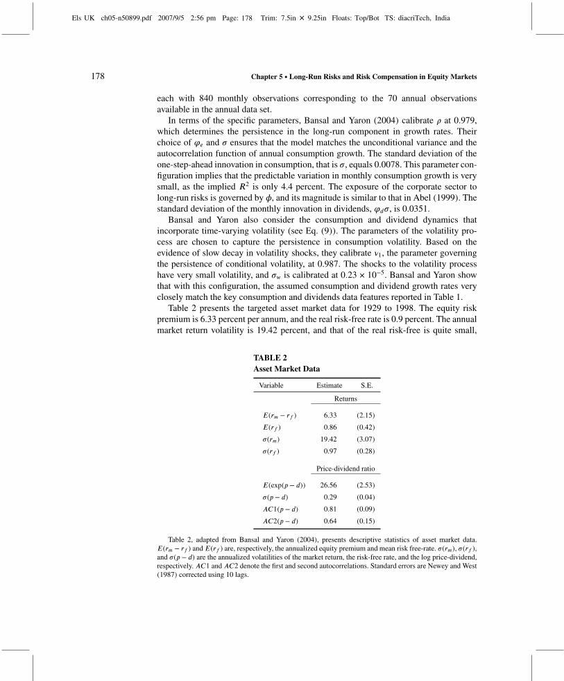
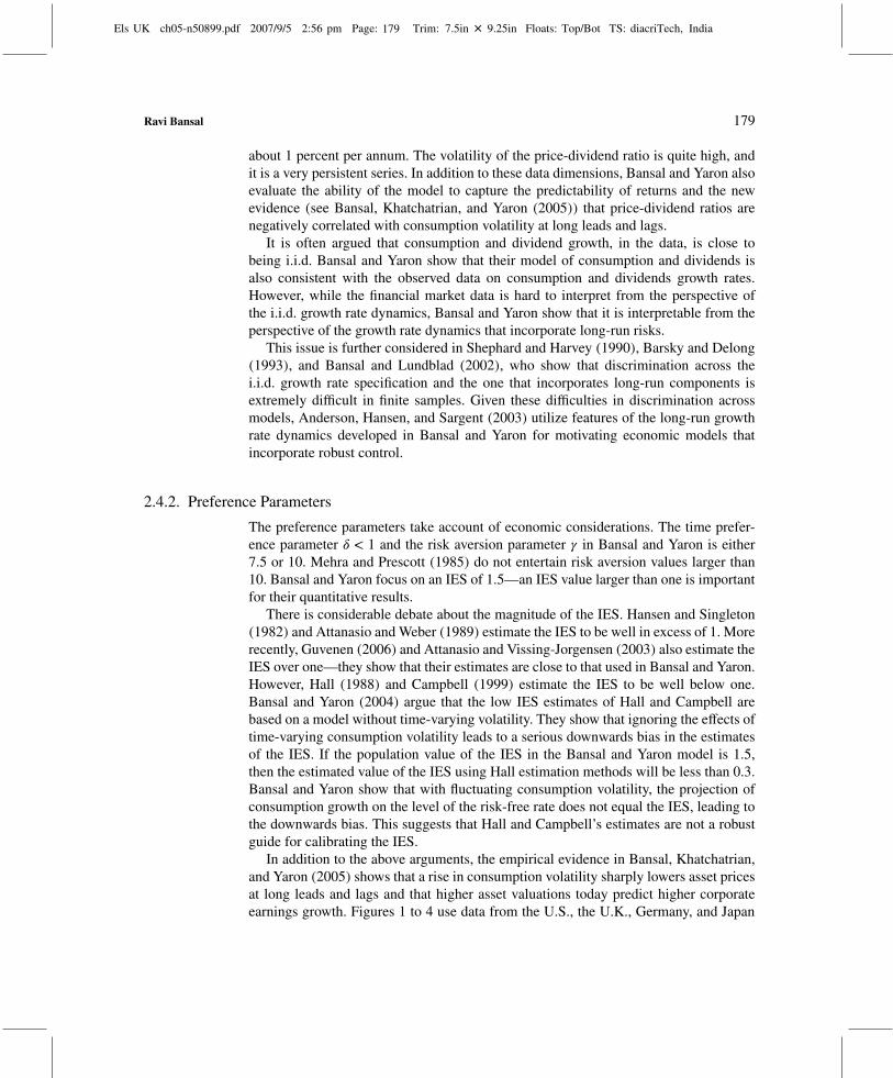
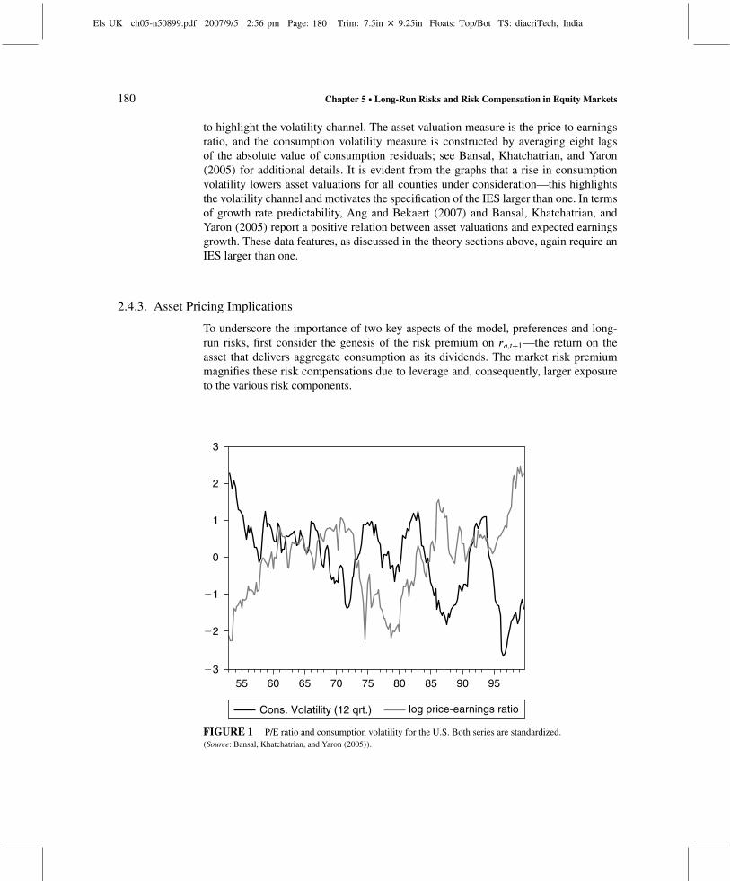
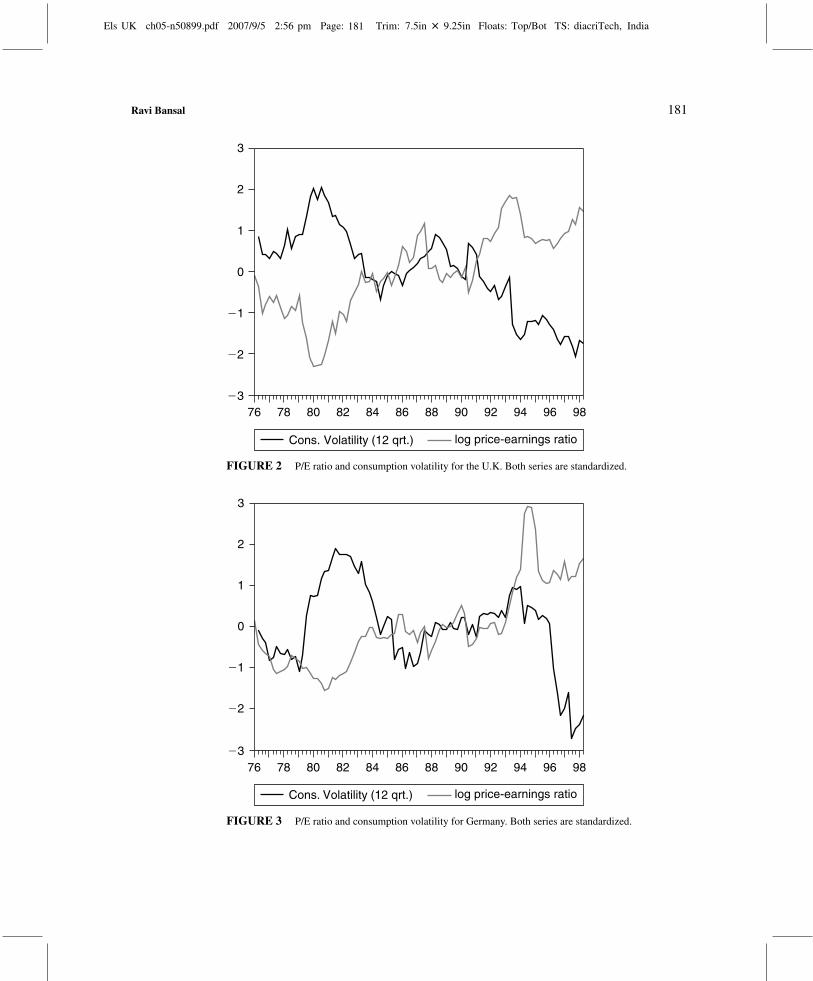
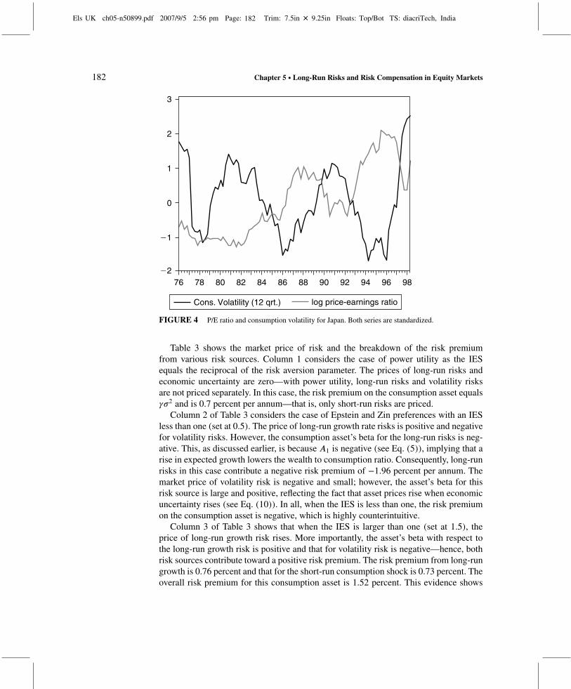
In addition to the above arguments, the empirical evidence in Bansal, Khatchatrian,and Yaron (2005) shows that a rise in consumption volatility sharply lowers asset pricesat long leads and lags and that higher asset valuations today predict higher corporateearnings growth. Figures 1 to 4 use data from the U.S., the U.K., Germany, and Japan
Els UK ch05-n50899.pdf 2007/9/5 2:56 pm Page: 180 Trim: 7.5in × 9.25in Floats: Top/Bot TS: diacriTech, India
180 Chapter 5 • Long-Run Risks and Risk Compensation in Equity Markets
to highlight the volatility channel. The asset valuation measure is the price to earningsratio, and the consumption volatility measure is constructed by averaging eight lagsof the absolute value of consumption residuals; see Bansal, Khatchatrian, and Yaron(2005) for additional details. It is evident from the graphs that a rise in consumptionvolatility lowers asset valuations for all counties under consideration—this highlightsthe volatility channel and motivates the specification of the IES larger than one. In termsof growth rate predictability, Ang and Bekaert (2007) and Bansal, Khatchatrian, andYaron (2005) report a positive relation between asset valuations and expected earningsgrowth. These data features, as discussed in the theory sections above, again require anIES larger than one.
2.4.3. Asset Pricing Implications
To underscore the importance of two key aspects of the model, preferences and long-run risks, first consider the genesis of the risk premium on ra,t+1—the return on theasset that delivers aggregate consumption as its dividends. The market risk premiummagnifies these risk compensations due to leverage and, consequently, larger exposureto the various risk components.
23
22
21
0
1
2
3
55 60 65 70 75 80 85 90 95
Cons. Volatility (12 qrt.) log price-earnings ratio
FIGURE 1 P/E ratio and consumption volatility for the U.S. Both series are standardized.(Source: Bansal, Khatchatrian, and Yaron (2005)).
Els UK ch05-n50899.pdf 2007/9/5 2:56 pm Page: 181 Trim: 7.5in × 9.25in Floats: Top/Bot TS: diacriTech, India
Ravi Bansal 181
23
22
21
0
1
2
3
76 78 80 82 84 86 88 90 92 94 96 98
Cons. Volatility (12 qrt.) log price-earnings ratio
FIGURE 2 P/E ratio and consumption volatility for the U.K. Both series are standardized.
23
22
21
0
1
2
3
76 78 80 82 84 86 88 90 92 94 96 98
Cons. Volatility (12 qrt.) log price-earnings ratio
FIGURE 3 P/E ratio and consumption volatility for Germany. Both series are standardized.
Els UK ch05-n50899.pdf 2007/9/5 2:56 pm Page: 182 Trim: 7.5in × 9.25in Floats: Top/Bot TS: diacriTech, India
182 Chapter 5 • Long-Run Risks and Risk Compensation in Equity Markets
Cons. Volatility (12 qrt.) log price-earnings ratio
22
21
0
1
2
3
76 78 80 82 84 86 88 90 92 94 96 98
FIGURE 4 P/E ratio and consumption volatility for Japan. Both series are standardized.
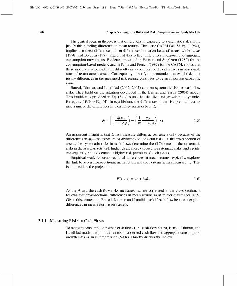
Table 3 shows the market price of risk and the breakdown of the risk premiumfrom various risk sources. Column 1 considers the case of power utility as the IESequals the reciprocal of the risk aversion parameter. The prices of long-run risks andeconomic uncertainty are zero—with power utility, long-run risks and volatility risksare not priced separately. In this case, the risk premium on the consumption asset equalsγσ2 and is 0.7 percent per annum—that is, only short-run risks are priced.
Column 2 of Table 3 considers the case of Epstein and Zin preferences with an IESless than one (set at 0.5). The price of long-run growth rate risks is positive and negativefor volatility risks. However, the consumption asset’s beta for the long-run risks is neg-ative. This, as discussed earlier, is because A1 is negative (see Eq. (5)), implying that arise in expected growth lowers the wealth to consumption ratio. Consequently, long-runrisks in this case contribute a negative risk premium of −1.96 percent per annum. Themarket price of volatility risk is negative and small; however, the asset’s beta for thisrisk source is large and positive, reflecting the fact that asset prices rise when economicuncertainty rises (see Eq. (10)). In all, when the IES is less than one, the risk premiumon the consumption asset is negative, which is highly counterintuitive.
Column 3 of Table 3 shows that when the IES is larger than one (set at 1.5), theprice of long-run growth risk rises. More importantly, the asset’s beta with respect tothe long-run growth risk is positive and that for volatility risk is negative—hence, bothrisk sources contribute toward a positive risk premium. The risk premium from long-rungrowth is 0.76 percent and that for the short-run consumption shock is 0.73 percent. Theoverall risk premium for this consumption asset is 1.52 percent. This evidence shows

Els UK ch05-n50899.pdf 2007/9/5 2:56 pm Page: 183 Trim: 7.5in × 9.25in Floats: Top/Bot TS: diacriTech, India
Ravi Bansal 183
TABLE 3Risk Components and Risk Compensation
ψ = 0.1 ψ = 0.5 ψ = 1.5
mprη 93.60 93.60 93.60
mpre 0.00 137.23 160.05
mprw 0.00 −27.05 −31.56
βη 1.00 1.00 1.00
βe −16.49 −1.83 0.61
βw 11026.45 1225.16 −408.39
prmη 0.73 0.73 0.73
prme 0.00 −1.96 0.76
prmw 0.00 −0.08 0.03
Table 3 presents model-implied components of the risk premium on the consumption asset for differentvalues of the intertemporal elasticity of the substitution parameter, ψ . All entries are based on γ = 10. Theparameters that govern the dynamics of the consumption process in Eq. (9) are identical to Bansal and Yaron(2004): ρ = 0.979, σ = 0.0078, ϕe = 0.044, ν1 = 0.987, σw = 0.23 × 10⁻⁵, and κ1 = 0.997. The first threerows report the annualized percentage prices of risk for innovations in consumption, the expected growth risk,and the consumption volatility risk—mprη , mpre, and mprw , respectively. These prices of risks correspond toannualized percentage values for λm,ησ, λm,eσ, λm,wσw in Eq. (11). The exposures of the consumption asset tothe three systematic risks, βη , βe, and βw , are presented in the middle part of the table. Total risk compensationin annual percentage terms for each risk is reported as prm∗ and equals the product of the price of risk, thestandard deviation of the shock, and the beta for the specific risk.
that an IES larger than one is required for the long-run and volatility risks to carry to apositive risk premium.
It is clear from Table 3 that the price of risk is highest for the long-run risks (seecolumns 2 and 3) and smallest for the volatility risks. A comparison of columns 2 and 3also shows that raising the IES increases the prices of long-run and volatility risks inabsolute value. The magnitudes reported in Table 3 are with ρ = 0.979—lowering thispersistence parameter also lowers the prices of long-run and volatility risks (in absolutevalue). Increasing the risk aversion parameter increases the prices of all consumptionrisks, as shown in Eq. (12). Hansen and Jagannathan (1991) document the importanceof the maximal Sharpe ratio, determined by the volatility of the IMRS, in assessing assetpricing models. Bansal and Yaron show that incorporating long-run risks increases themaximal Sharpe ratio for their model, and it satisfies the non-parametric bounds ofHansen and Jagannathan (1991).
The risk premium on the market portfolio (i.e., the dividend asset) is also affected bythe presence of long-run risks. To underscore their importance, assume that consump-tion and dividend growth rates are i.i.d. This shuts off the long-run risk channel. Themarket risk premium in this case is
Et(rm,t+1 − rf ,t) = γCov(gt+1, gd,t+1) − 0.5Var(gd,t+1), (14)
Els UK ch05-n50899.pdf 2007/9/5 2:56 pm Page: 184 Trim: 7.5in × 9.25in Floats: Top/Bot TS: diacriTech, India
184 Chapter 5 • Long-Run Risks and Risk Compensation in Equity Markets
and market return volatility equals the dividend growth rate volatility. If shocks toconsumption and dividends are uncorrelated, then the geometric risk premium is neg-ative and equals −0.5Var(gd,t+1). If the correlation between monthly consumption anddividend growth is 0.25, then the equity premium is 0.08 percent per annum—similarto the evidence documented in Mehra and Prescott (1985) and Weil (1989). Bansaland Yaron show that incorporating long-run growth rate risks (see Eq. (4)) producesan annual equity risk premium of 4.2 percent and a risk-free rate of 1.34 percent alongwith market return and price-dividend volatility of 16.21 percent and 0.16, respectively.These are fairly comparable to what we see in the data (see Table 2) and highlight theimportance of long-run growth rate risks.
Bansal and Yaron show that the full model that incorporates long-run growth raterisks and fluctuating economic uncertainty provides a very close match to the asset mar-ket data reported in Table 2. That is, this model can account for the low risk-free rate,high equity premium, high asset price volatility, and low risk-free rate volatility. Thismodel also quantitatively matches additional data features, such as (i) predictability ofreturns at short and long horizons using the dividend yield as a predictive variable,(ii) time-varying and persistent market return volatility, (iii) negative correlationbetween market return and volatility shocks, i.e., the volatility feedback effect, (iv) neg-ative relation between consumption volatility and asset prices at long leads and lags,documented in Bansal, Khatchatrian, and Yaron (2005).
In all, this evidence shows that incorporating long-run risks in growth rates andfluctuating economic uncertainty can help interpret a wide array of the asset marketpuzzles.
2.4.4. Value of Contingent Claims and Macro Markets
Using the Efficient Method of Moments (EMM), Bansal, Gallant, and Tauchen (2007)consider the implications of alternative asset pricing models presented in Bansal andYaron and in Campbell and Cochrane (1999). A unique dimension of this paper is thatthey model the consumption and dividends as being cointegrated, a feature that is miss-ing in earlier work of Campbell and Cochrane (1999) and Bansal and Yaron (2004).Bansal, Gallant, and Tauchen evaluate the value of contingent claims on the aggregatewealth of the economy. This is a first step in assessing the plausibility of introducingcontingent claims on macro variables for better risk sharing, as espoused by Shiller(1998). This valuation exercise also helps understand the different channels operatingin these models.
Bansal, Gallant, and Tauchen document large differences in the prices of put optionson the consumption claim across the two asset pricing models. The volatility of theconsumption claim in the Bansal and Yaron model is about one-fourth that of the marketreturn, while in the Campbell and Cochrane model it is about as volatile as the marketportfolio.
Els UK ch05-n50899.pdf 2007/9/5 2:56 pm Page: 185 Trim: 7.5in × 9.25in Floats: Top/Bot TS: diacriTech, India
Ravi Bansal 185
3. CROSS-SECTIONAL IMPLICATIONS
3.1. Value, Momentum, Size, and the Cross-Sectional Puzzle
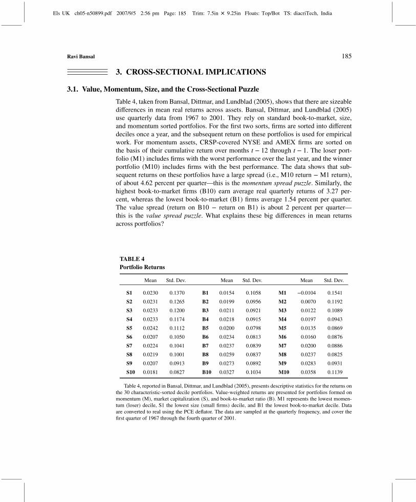
Table 4, taken from Bansal, Dittmar, and Lundblad (2005), shows that there are sizeabledifferences in mean real returns across assets. Bansal, Dittmar, and Lundblad (2005)use quarterly data from 1967 to 2001. They rely on standard book-to-market, size,and momentum sorted portfolios. For the first two sorts, firms are sorted into differentdeciles once a year, and the subsequent return on these portfolios is used for empiricalwork. For momentum assets, CRSP-covered NYSE and AMEX firms are sorted onthe basis of their cumulative return over months t − 12 through t − 1. The loser port-folio (M1) includes firms with the worst performance over the last year, and the winnerportfolio (M10) includes firms with the best performance. The data shows that sub-sequent returns on these portfolios have a large spread (i.e., M10 return − M1 return),of about 4.62 percent per quarter—this is the momentum spread puzzle. Similarly, thehighest book-to-market firms (B10) earn average real quarterly returns of 3.27 per-cent, whereas the lowest book-to-market (B1) firms average 1.54 percent per quarter.The value spread (return on B10 − return on B1) is about 2 percent per quarter—this is the value spread puzzle. What explains these big differences in mean returnsacross portfolios?
TABLE 4Portfolio Returns
Mean Std. Dev. Mean Std. Dev. Mean Std. Dev.
S1 0.0230 0.1370 B1 0.0154 0.1058 M1 −0.0104 0.1541
S2 0.0231 0.1265 B2 0.0199 0.0956 M2 0.0070 0.1192
S3 0.0233 0.1200 B3 0.0211 0.0921 M3 0.0122 0.1089
S4 0.0233 0.1174 B4 0.0218 0.0915 M4 0.0197 0.0943
S5 0.0242 0.1112 B5 0.0200 0.0798 M5 0.0135 0.0869
S6 0.0207 0.1050 B6 0.0234 0.0813 M6 0.0160 0.0876
S7 0.0224 0.1041 B7 0.0237 0.0839 M7 0.0200 0.0886
S8 0.0219 0.1001 B8 0.0259 0.0837 M8 0.0237 0.0825
S9 0.0207 0.0913 B9 0.0273 0.0892 M9 0.0283 0.0931
S10 0.0181 0.0827 B10 0.0327 0.1034 M10 0.0358 0.1139
Table 4, reported in Bansal, Dittmar, and Lundblad (2005), presents descriptive statistics for the returns onthe 30 characteristic-sorted decile portfolios. Value-weighted returns are presented for portfolios formed onmomentum (M), market capitalization (S), and book-to-market ratio (B). M1 represents the lowest momen-tum (loser) decile, S1 the lowest size (small firms) decile, and B1 the lowest book-to-market decile. Dataare converted to real using the PCE deflator. The data are sampled at the quarterly frequency, and cover thefirst quarter of 1967 through the fourth quarter of 2001.
Els UK ch05-n50899.pdf 2007/9/5 2:56 pm Page: 186 Trim: 7.5in × 9.25in Floats: Top/Bot TS: diacriTech, India
186 Chapter 5 • Long-Run Risks and Risk Compensation in Equity Markets
The central idea, in theory, is that differences in exposure to systematic risk shouldjustify this puzzling difference in mean returns. The static CAPM (see Sharpe (1964))implies that these differences mirror differences in market betas of assets, while Lucas(1978) and Breeden (1979) argue that they reflect differences in exposure to aggregateconsumption movements. Evidence presented in Hansen and Singleton (1982) for theconsumption-based models, and in Fama and French (1992) for the CAPM, shows thatthese models have considerable difficulty in accounting for the differences in observablerates of return across assets. Consequently, identifying economic sources of risks thatjustify differences in the measured risk premia continues to be an important economicissue.
Bansal, Dittmar, and Lundblad (2002, 2005) connect systematic risks to cash-flowrisks. They build on the intuition developed in the Bansal and Yaron (2004) model.This intuition is provided in Eq. (8). Assume that the dividend growth rate dynamicsfor equity i follow Eq. (4). In equilibrium, the differences in the risk premium acrossassets mirror the differences in their long-run risks beta, βi,
βi =
[(φiϕe
1 − κ1ρ
)−(
1ψ
ϕe1 − κ1ρ
)]κ1. (15)
An important insight is that βi risk measure differs across assets only because of thedifferences in φi—the exposure of dividends to long-run risks. In the cross section ofassets, the systematic risks in cash flows determine the differences in the systematicrisks in the asset. Assets with higher φi are more exposed to systematic risks, and agents,consequently, should demand a higher risk premium of such assets.
Empirical work for cross-sectional differences in mean returns, typically, exploresthe link between cross-sectional mean return and the systematic risk measure, βi. Thatis, it considers the projection
E(ri,t+1) = λ0 + λcβi. (16)
As the βi and the cash-flow risks measures, φi, are correlated in the cross section, itfollows that cross-sectional differences in mean returns must mirror differences in φi.Given this connection, Bansal, Dittmar, and Lundblad ask if cash-flow betas can explaindifferences in mean return across assets.
3.1.1. Measuring Risks in Cash Flows
To measure consumption risks in cash flows (i.e., cash-flow betas), Bansal, Dittmar, andLundblad model the joint dynamics of observed cash flow and aggregate consumptiongrowth rates as an autoregression (VAR). I briefly discuss this below.

Els UK ch05-n50899.pdf 2007/9/5 2:56 pm Page: 187 Trim: 7.5in × 9.25in Floats: Top/Bot TS: diacriTech, India
Ravi Bansal 187
For any asset i, using the return approximation in Eq. (3), the log price minus logcash flow, pi,t − di,t, satisfies
pi,t − di,t =κi,0
1 − κi,1+ Et
[ ∞∑j=0
κj
i,1gi,t+1+j −∞∑j=0
κj
i,1ri,t+1+j
]. (17)
The log price− cash flow ratio is determined by the discounted expected cash-flowgrowth rates and discounted expected returns. The discount rate, κi,1, is less than oneby construction. Exploiting (3) and (17), it follows that return innovations are related toinnovations in expectations of future cash flows and returns:
ri,t − Et−1[ri,t] = {Et − Et−1}[ ∞∑j=0
κj
i,1gi,t+j
]− {Et − Et−1}
[ ∞∑j=1
κj
i,1ri,t+j
]
= ηgi,t − ηei,t. (18)
The piece ηgi,t = {Et − Et−1}[∑∞j=0 κ
j
i,1gi,t+j] is cash-flow news and represents the revi-sion in expectations of the sum of future dividend growth rates. Analogously, ηei,trepresents discount rate news.
Given the return decomposition, the consumption beta can be described as
βi =Cov(ri,t − Et−1(ri,t), ηt)
Var(ηt)=
Cov(ηgi,t − ηei,t, ηt)Var(ηt)
= βi,g − βi,e, (19)
where ηt is the time t innovation in consumption growth. The consumption beta isgoverned by two components—the cash-flow beta and the beta of discount rate news.Bansal, Dittmar, and Lundblad ask if the cash-flow beta, βi,g , can explain differences inrisk premia across assets.
To estimate the cash-flow betas, they model the de-meaned log consumption growth,gc,t, as a simple AR(1) process:
gc,t = ρcgc,t−1 + ηt, (20)
with ρc being the AR(1) coefficient and ηt the consumption news at date t. Further,they assume that the relationship between de-meaned dividend and consumption growthrates is
gi,t = φi
( 1K
K∑k=1
gc,t−k)+ ui,t, (21)
ui,t =L∑j=1
ρj,iui,t−j + ζi,t. (22)
Els UK ch05-n50899.pdf 2007/9/5 2:56 pm Page: 188 Trim: 7.5in × 9.25in Floats: Top/Bot TS: diacriTech, India
188 Chapter 5 • Long-Run Risks and Risk Compensation in Equity Markets
The expression 1/K∑Kk=1 gc,t−k represents a trailing K-period moving average of past
consumption growth—this a measure of xt discussed above in the Bansal and Yaron(2004) model. The parameter φi measures the leverage of the dividends, as discussedin Eq. (4). This specification allows for cash-flow growth rates to depend on the currentconsumption innovation through the process for ζi,t. This contemporaneous covarianceis reflected in the measured cash-flow betas.
Equations (20), (21), and (22) characterize a simple VAR. The q-vector, Yt, is
Yt = [gi,t ui,t · · · ui,t−(L−1) gc,t · · · gc,t−(K−1)]′, (23)
and the dynamics of the state variables and portfolio cash flow growth can then beexpressed as
Yt = AYt−1 + vt, (24)
where A is the q × q matrix of coefficients. Let the first element of Yt be gi,t such thate′1zt = gi,t, where e1 is a q × 1 vector with first element 1 and remaining elements 0.From Eq. (18), it follows that ηgi,t is equal to
ηgi,t = {Et − Et−1}[ ∞∑j=0
κj
i,1gi,t+j
]
= e′1[ ∞∑j=0
κj
i,1Ajvt
]
= e′1[I − κi,1A
]−1vt. (25)
This residual represents the innovation to current and expected future cash-flow growthrates. The exposure of this innovation to consumption growth is measured by projectingit on the innovation in consumption growth, specifically,
ηgi,t = βi,gηt + ξgi,t. (26)
The resulting projection coefficient, βi,g , is the asset’s cash-flow beta developed inBansal, Dittmar, and Lundblad (2002, 2005). Note that if ui,t is uncorrelated with con-sumption innovation, then the cross-sectional differences in the cash-flow beta based onEq. (26) solely reflect differences in φi. Hence, if one imposes the restriction that ui,tis uncorrelated with consumption innovations, then it is sufficient to focus on φi. Giventhe cash flow’s consumption beta, Bansal, Dittmar, and Lundblad run the cross-sectionalregression,
E[Ri,t] = λ0 + βi,gλc (27)
to evaluate the empirical plausibility of the cash-flow beta model.
Els UK ch05-n50899.pdf 2007/9/5 2:56 pm Page: 189 Trim: 7.5in × 9.25in Floats: Top/Bot TS: diacriTech, India
Ravi Bansal 189
3.1.2. Dividends and Cash Flows
Bansal, Dittmar, and Lundblad measure the cash flows as dividends for each portfolioin a standard manner, specifically,
Rt+1 = ht+1 + yt+1, (28)
where ht+1 is the price appreciation and yt+1 the dividend yield (i.e., dividends at datet + 1 per dollar invested at date t). We observe Rt+1 (RET in CRSP terminology) andthe price gain series ht+1 (RETX) for each portfolio; hence, yt+1 = Rt+1 − ht+1. Thelevel of the dividends we use in the paper is computed as
Dt+1 = yt+1Vt, (29)
where
Vt+1 = ht+1Vt, (30)
with V0 = 1. Hence, the dividend series that we use, Dt, corresponds to the total cashdividends given out by a mutual fund at t that extracts the dividends and reinvests thecapital gains. The ex-dividend value of the mutual fund is Vt, and the per dollar returnfor the investors in the mutual fund is
Rt+1 =Vt+1 +Dt+1
Vt= ht+1 + yt+1. (31)
From this equation, it is evident that Vt is the discounted value of the dividends thatwe use.
Bansal, Dittmar, and Lundblad (2005) also use repurchase adjusted dividends andearnings as a measure of cash flows. The empirical evidence is similar to that foundusing cash dividends. More recently, Bansal and Yaron (2006) use market clearingrestrictions as a way to identify the appropriate trading strategy to use for measuringaggregate dividends. This measure, relative to the per share-based traditionally usedmeasure (as in Eq. (29)), incorporates the relative shift in scale of the different sectorsand yields different insights into the sources of the asset price variation.
3.1.3. Performance of Cash-Flow Beta Model
As predicted by the Bansal and Yaron (2004) model, the consumption leverage ofdivided growth rates has great explanatory power. Bansal, Dittmar, and Lundblad showthat using φi or βi,g as the risk measure yields a highly positive and significant price ofrisk estimates of λc, and the cross-sectional R2 are well in excess of 60 percent. Usingan alternative asset menu of 25 portfolios based on the Fama–French 5 × 5 two-waysort on market capitalization and book-to-market value also yields comparable results.Bansal, Dittmar, and Lundblad (2002, 2005) also ask if the cash-flow risks are relatedto the long-run risks of Bansal and Yaron (2004). They show that when, in Eq. (21),K = 1, the consumption risks are largely short-run risks and the cash-flow betas are notable to capture the cross-sectional differences in risk premia. Increasing K, and hence
Els UK ch05-n50899.pdf 2007/9/5 2:56 pm Page: 190 Trim: 7.5in × 9.25in Floats: Top/Bot TS: diacriTech, India
190 Chapter 5 • Long-Run Risks and Risk Compensation in Equity Markets
exaggerating the long-run risks, is important for the success of the cash-flow betas incapturing differences in mean returns across assets.
In contrast, alternative models find it quite hard to explain the differences in meanreturns for the 30 asset menus used in Bansal, Dittmar, and Lundblad. The standardconsumption betas (i.e., C-CAPM) and the market-based CAPM asset betas have closeto zero explanatory power. The R2 for the C-CAPM is 2.7 percent, and that for the mar-ket CAPM is 6.5 percent, with an implausible negative slope coefficient. The Famaand French three-factor empirical specification also generates point estimates withnegative, and difficult to interpret, price of risk for the market and size factors—thecross-sectional R2 is about 36 percent. Compared to all these models, the cash-flowrisks model of Bansal, Dittmar, and Lundblad is able to capture a significant portion ofthe differences in risk premia across assets.
In addition, Bansal, Dittmar, and Lundblad (2001) and Bansal, Dittmar, and Kiku(2007) also consider a risk measure based on stochastic cointegration between thelog level of dividends and consumption. This risk measure is estimated via the pro-jection of the deterministically de-trended level of log dividends on the de-trendedlevel of log consumption. Bansal, Dittmar, and Kiku (2007) derive new results thatlink this cointegration parameter to consumption betas by investment horizon and eval-uate the ability of their model to explain differences in mean returns for differenthorizons. Hansen, Heaton, and Li (2006) inquire about the robustness of the stochas-tic cointegration-based risk measures considered in Bansal, Dittmar, and Lundblad(2001). Bansal, Dittmar, and Kiku provide new evidence regarding the robustness of thestochastic cointegration-based measures of permanent risks in equity markets. Parkerand Julliard (2005) evaluate if long-run risks in aggregate consumption can accountfor the cross section of expected returns. Malloy, Moskowitz, and Vissing-Jørgensen(2006) evaluate if long-run risks in the consumption of stockholders has greater abil-ity to explain the cross section of equity returns, relative to aggregate consumptionmeasures.
Bansal, Dittmar, and Lundblad (2005) also discuss why cash-flow risks may cap-ture the differences in risk premia when standard consumption betas fail to do so. TheBansal and Yaron model helps explain why this may be the case—in this model of mul-tiple risks, the consumption beta is not sufficient to capture differences in risk premiaacross assets. Imagine that risk premia are determined by Eq. (13), that is, there aremultiple sources of risks. Let the shocks to the various risk sources be correlated, andthen the standard consumption beta will measure a weighted linear combination of thethree different betas. While each individual beta may be important in capturing the riskpremia across assets—a weighted linear combination may fail to do so. Bansal, Dittmar,and Lundblad (2005) provide simulation evidence wherein the C-CAPM betas fail toexplain the difference in mean returns across assets, while the cash-flow betas capture asizable portion of the cross-sectional differences in mean returns.
The approach pursued in Bansal, Dittmar, and Lundblad (2005) derives constant riskmeasures. Jagannathan and Wang (1996) and Lettau and Ludvigson (2001) focus ontime-varying return betas. Deriving and measuring time-varying cash-flow betas wouldbe a valuable extension for future research.
Els UK ch05-n50899.pdf 2007/9/5 2:56 pm Page: 191 Trim: 7.5in × 9.25in Floats: Top/Bot TS: diacriTech, India
Ravi Bansal 191
4. CONCLUSION
The work of Bansal and Lundblad (2002), Bansal and Yaron (2004), and Bansal,Gallant, and Tauchen (2004) show that long-run growth rate risks and varying eco-nomic uncertainty are important for quantitatively interpreting financial markets. Thesepapers argue that investors care about the long-run growth prospects and the uncertaintysurrounding the growth rate. Risks associated with changing long-run growth prospectsand varying economic uncertainty drive the level of returns and asset price volatility infinancial markets.
A key issue in terms of the preferences of investors is their attitude toward riskas measured by risk aversion and the magnitude of the parameter that determinesintertemporal substitution. Based on recent empirical evidence on the magnitude ofthe IES, and on its economic implications for asset markets, Bansal and Yaron arguethat the IES should be larger than one. They show that only when the IES is largerthan one does increased economic uncertainty translate into a drop in asset prices.Bansal, Khatchatrian, and Yaron (2005) find very robust empirical evidence that a risein economic uncertainty lowers asset prices across different samples and countries. Thisevidence suggests that the IES may indeed be larger than one.
Bansal, Dittmar, and Lundblad (2002, 2005) show that long-run risks in cash flowsof portfolios should explain differences in mean returns across assets. They measurecash-flow risks via estimating cash-flow betas and find that the consumption risks incash flows of portfolios explain very well the differences in mean returns across equityportfolios. Using cash flows and consumption, they devise ways to measure cash-flowbetas that capture systematic risks in cash flows. These risk measures, they find, pro-vide very sharp information about differences in risk premia across assets. They showthat the cash-flow betas can explain the differences in mean returns for value, size, andmomentum sorted portfolios.
All of this evidence and the economics underlying it support the view that the long-run risks and uncertainty channel contain very valuable insights about the workings offinancial markets.
References
Abel, A. B. Risk premia and term premia in general equilibrium. Journal of Monetary Economics 43 (1999):3–33.
Anderson, E., L. P. Hansen, and T. Sargent. A quartet of semi-groups for model specification, robustness,prices of risk and model detection. Journal of the European Economic Association 1 (2003): 68–123.
Ang, A., and G. Bekaert. Stock return predictability: Is it there? Review of Financial Studies 20 (2007):651–707.
Ansley, C. F., and P. Newbold. Finite sample properties of estimators for autoregressive moving averagemodels. Journal of Econometrics 13 (1980): 159–184.
Attanasio, P. O., and A. Vissing-Jorgensen. Stock market participation, intertemporal substitution and riskaversion. American Economic Review 93 (2003): 383–391.
Attanasio, P. O., and G. Weber. Intertemporal substitution, risk aversion and the Euler equation forconsumption. Economic Journal 99 (1989): 59–73.

Els UK ch05-n50899.pdf 2007/9/5 2:56 pm Page: 192 Trim: 7.5in × 9.25in Floats: Top/Bot TS: diacriTech, India
192 Chapter 5 • Long-Run Risks and Risk Compensation in Equity Markets
Bansal, R., R. F. Dittmar, and D. Kiku. Cointegration and consumption risks in asset returns. Review ofFinancial Studies forthcoming (2007).
Bansal, R., R. F. Dittmar, and C. Lundblad. Consumption, dividends and the cross-section of equity returns.Working paper. Duke University (2001).
Bansal, R., R. F. Dittmar, and C. Lundblad. Interpreting risk premia across size, value, and industry portfolios.Working paper. Duke University (2002).
Bansal, R., R. F. Dittmar, and C. Lundblad. Consumption, dividends and the cross-section of equity returns.Journal of Finance 60 (2005): 1639–1672.
Bansal, R., R. A. Gallant, and G. Tauchen. Rational pessimism, rational exuberance, and asset pricing models.Review of Economic Studies forthcoming (2007).
Bansal, R., V. Khatchatrian, and A. Yaron. Interpretable asset markets? European Economic Review49 (2005): 531–560.
Bansal, R., and C. Lundblad. Market efficiency, asset returns, and the size of the risk premium in global equitymarkets. Journal of Econometrics 109 (2002): 195–237.
Bansal, R., and A. Yaron. Risks for the long run: A potential resolution of asset pricing puzzles. Journal ofFinance 59 (2004): 1481–1509.
Bansal, R., and A. Yaron. The asset pricing-macro nexus and return-cash flow predictability. Working paper.Duke University (2006).
Barsky, R., and B. J. DeLong. Why does the stock market fluctuate? Quarterly Journal of Economics108 (1993): 291–312.
Breeden, D. T. An intertemporal asset pricing model with stochastic consumption and investment opportuni-ties. Journal of Financial Economics 7 (1979): 265–296.
Campbell, J. Y. Asset prices, consumption and the business cycle, in J. B. Taylor, and M. Woodford, eds.,Handbook of Macroeconomics, Volume 1. Elsevier Science, North-Holland, Amsterdam (1999).
Campbell, J. Y., and J. H. Cochrane. By force of habit: A consumption-based explanation of aggregate stockmarket behavior. Journal of Political Economy 107 (1999): 205–251.
Campbell, J. Y., and R. J. Shiller. The dividend-price ratio and expectations of future dividends and discountfactors. Review of Financial Studies 1 (1988): 195–227.
Cecchetti, S. G., P.-S., Lam, and N. C. Mark. The equity premium and the risk free rate: Matching themoments. Journal of Monetary Economics 31 (1993): 21–46.
Cochrane, J. H. How big is the random walk in GNP? Journal of Political Economy 96 (1988): 893–920.Epstein, L., and S. Zin. Substitution, risk aversion and the temporal behavior of consumption and asset returns:
A theoretical framework. Econometrica 57 (1989): 937–969.Fama, E., and K. French. The cross-section of expected stock returns. Journal of Finance 59 (1992): 427–465.Guvenen, F. Reconciling conflicting evidence on the elasticity of intertemporal substitution: A macroeco-
nomic perspective. Journal of Monetary Economics 53 (2006): 1451–1472.Hall, R. E. Intertemporal substitution in consumption. Journal of Political Economy 96 (1988): 339–357.Hansen, L. P., J. Heaton, and N. Li. Consumption strikes back? Measuring long-run risk. Working paper.
University of Chicago (2006).Hansen, L. P., and R. Jagannathan. Implications of security market data for models of dynamic economies,
Journal of Political Economy 99 (1991): 225–262.Hansen, L. P., and K. Singleton. Generalized instrumental variables estimation of nonlinear rational
expectations models. Econometrica 50 (1982): 1269–1286.Hurwicz, L. Least square bias in time series, in T. Koopmans, ed., Statistical Inference in Dynamic Economic
Models. Wiley Press, New York (1950).Jagannathan, R., and Z. Wang. The conditional CAPM and the cross-section of expected returns. Journal of
Finance 51 (1996): 3–54.Judd, K. Numerical Methods in Economics. MIT Press, Cambridge, MA (1998).Kandel, S., and R. F. Stambaugh. Asset returns and intertemporal preferences. Journal of Monetary
Economics 27 (1991): 39–71.LeRoy, S., and R. Porter. The present value relation: Tests based on implied variance bounds. Econometrica
49 (1981): 555–574.

Els UK ch05-n50899.pdf 2007/9/5 2:56 pm Page: 193 Trim: 7.5in × 9.25in Floats: Top/Bot TS: diacriTech, India
Ravi Bansal 193
Lettau, M., and S. Ludvigson. Resurrecting the (C)CAPM: A cross-sectional test when risk premia aretime-varying. Journal of Political Economy 109 (2001): 1238–1287.
Lucas, R. Asset prices in an exchange economy. Econometrica 46 (1978): 1429–1446.Malloy, C. J., T. J. Moskowitz, and A. Vissing-Jorgensen. Long-run stockholder consumption risk and asset
returns. Working paper. University of Chicago (2006).Mehra, R., and E. C. Prescott. The equity premium: A puzzle. Journal of Monetary Economics 15 (1985):
145–161.Newey, W. K., and K. D. West. A simple, positive semi-definite, heteroskedasticity and autocorrelation
consistent covariance matrix. Econometrica 55 (1987): 703–708.Parker, J., and C. Julliard. Consumption risk and the cross-section of expected returns. Journal of Political
Economy 113 (2005): 185–222.Sharpe, W. Capital asset prices: A theory of market equilibrium under conditions of risk. Journal of Finance
19 (1964): 425–442.Shephard, N. G., and A. C. Harvey. On the probability of estimating a deterministic component in the local
level model, Journal of Time Series Analysis 11 (1990): 339–347.Shiller, R. J. Do stock prices move too much to be justified by subsequent changes in dividends? American
Economic Review 71 (1981): 421–436.Shiller, R. J. Macro markets: Creating institutions for managing society’s largest economic risks. Oxford
University Press, New York (1998).Weil, P. The equity premium puzzle and the risk-free rate puzzle. Journal of Monetary Economics 24 (1989):
401–421.

Els UK Ch05-Discussion-N50899.pdf 2007/9/5 2:56 pm Page: 194 Trim: 7.5in × 9.25in Floats: Top/Bot TS: diacriTech, India
194 Chapter 5 • Long-Run Risks and Risk Compensation in Equity Markets
Discussion of “Long-Run Risks andRisk Compensation in Equity Markets”
John HeatonGraduate School of Business, University of Chicago, and NBER
1. SUMMARY
Bansal and his co-authors have produced a series of important and provocative papersthat demonstrate how low-frequency risk can provide a justification for observed riskpremia. Bansal summarizes this work and helps us understand the linkages betweenlong-run risk in consumption and long-run risk in financial securities. Since he doessuch a nice job of explaining the economics of the approach, I focus on a few issuesraised by Bansal’s work and by some of my own.
2. A LOW-FREQUENCY COMPONENT IN CONSUMPTION?
An important aspect of the model of Bansal and Yaron (2004) is the presence of a low-frequency component in aggregate consumption. Shocks to the level of consumption arepersistent, as are shocks to volatility. A substantial and time-varying equity premiumresults when dividends display exposure to the shocks. It is natural to ask whether thereis any empirical support for the assumed model of consumption.
As Bansal argues, one piece of evidence may come from financial markets. Agentscould use the model’s structure along with signals from asset prices to detect thelow-frequency component. This may take the rational expectations assumption to anuntenable position, however. Unless agents directly observe the low-frequency shocksdriving consumption, it is not clear how the shocks could be reflected in security prices.Appealing to the standard idea that the econometrician observes a smaller informationset than agents is also a little delicate in this context. In the model of preferences con-sidered by Bansal and Yaron (2004), the exact conditioning information of the agents isneeded in order to derive the implications of the model.

Els UK Ch05-Discussion-N50899.pdf 2007/9/5 2:56 pm Page: 195 Trim: 7.5in × 9.25in Floats: Top/Bot TS: diacriTech, India
John Heaton 195
An interesting way of introducing a concern for low-frequency components, evenwhen agents have a hard time detecting those components, is provided by the recentwork of Hansen and Sargent (2007). In their work the representative agent is uncertainabout the probability model generating consumption. There are two alternative models:one where consumption is not predictable and one where consumption is predictable.Because the agent is worried about model uncertainty, she acts as if there is a very highprobability attached to the model with predictable consumption. This model generatesboth the high-risk premia consistent with a low-frequency component in consumption,and consumption dynamics that are difficult to distinguish from an i.i.d. model.
There is evidence in the literature for an important predictable low-frequency com-ponent to consumption. This evidence is typically obtained using additional variables topredict consumption along with plausible economic linkages across variables. Examplesinclude the work of Fisher (2006) and Mulligan (2002). In Hansen et al. (2006a) weconsider a bivariate model for aggregate consumption and aggregate corporate earnings.We present evidence that corporate earnings are co-integrated with aggregate consump-tion as predicted by most models of business cycles and economic growth. Underthe co-integration assumption, corporate earnings reveal important long-run shocks toconsumption.
To illustrate this, Figure 1 reports the impulse response of aggregate consumptionto the two shocks in the model.1 We call the first shock a “consumption shock”; itimpacts both consumption and earnings contemporaneously. In contrast, the secondshock impacts earnings contemporaneously but has no immediate impact on consump-tion. We call this shock an “earnings shock.” Shocks to corporate earnings predictconsumption over many quarters and reveal an important low-frequency componentof consumption similar to the setup considered by Bansal and Yaron (2004).
3. PREFERENCES
In his work, Bansal employs the recursive specification of preferences developed byKreps and Porteus (1978), Epstein and Zin (1989b), Weil (1990), and others. In thecontext of models with long-run consumption risk, this model of preferences is usefulbecause it induces a concern for the resolution of uncertainty. In a standard model withtime-additive CRRA utility, risk prices are determined by risk aversion and the one-period or instantaneous impact of shocks on consumption. With recursive preferences,the long-run impact of shocks on consumption also influences risk prices. Shocks thatstrongly predict future consumption have larger risk premia.
Calibration of the models considered by Bansal does run into the problem that con-sumption is not that volatile even in the long run. Large levels of risk aversion aretypically needed to fit aggregate and cross-sectional risk premia. An advantage of theassumption of recursive preference is that the effects of high risk aversion on the level of
1This figure is taken from Hansen et al. (2006b).
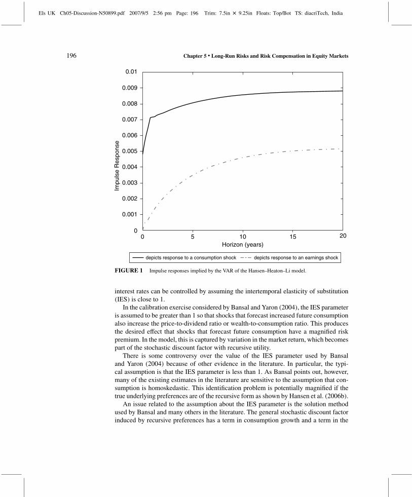
Els UK Ch05-Discussion-N50899.pdf 2007/9/5 2:56 pm Page: 196 Trim: 7.5in × 9.25in Floats: Top/Bot TS: diacriTech, India
196 Chapter 5 • Long-Run Risks and Risk Compensation in Equity Markets
0 5 10 15 200
0.001
0.002
0.003
0.004
0.005
0.006
0.007
0.008
0.009
0.01
Horizon (years)
Impu
lse
Res
pons
e
depicts response to a consumption shock depicts response to an earnings shock
FIGURE 1 Impulse responses implied by the VAR of the Hansen–Heaton–Li model.
interest rates can be controlled by assuming the intertemporal elasticity of substitution(IES) is close to 1.
In the calibration exercise considered by Bansal and Yaron (2004), the IES parameteris assumed to be greater than 1 so that shocks that forecast increased future consumptionalso increase the price-to-dividend ratio or wealth-to-consumption ratio. This producesthe desired effect that shocks that forecast future consumption have a magnified riskpremium. In the model, this is captured by variation in the market return, which becomespart of the stochastic discount factor with recursive utility.
There is some controversy over the value of the IES parameter used by Bansaland Yaron (2004) because of other evidence in the literature. In particular, the typi-cal assumption is that the IES parameter is less than 1. As Bansal points out, however,many of the existing estimates in the literature are sensitive to the assumption that con-sumption is homoskedastic. This identification problem is potentially magnified if thetrue underlying preferences are of the recursive form as shown by Hansen et al. (2006b).
An issue related to the assumption about the IES parameter is the solution methodused by Bansal and many others in the literature. The general stochastic discount factorinduced by recursive preferences has a term in consumption growth and a term in the

Els UK Ch05-Discussion-N50899.pdf 2007/9/5 2:56 pm Page: 197 Trim: 7.5in × 9.25in Floats: Top/Bot TS: diacriTech, India
John Heaton 197
“continuation value” due to future consumption. Following earlier work by Epstein andZin (1989a), shocks to the “continuation value” are replaced by shocks to the returnto holding a claim on aggregate consumption (the “market” return). This generates aproper solution to the model except for the case of logarithmic intertemporal risk pref-erences (IES = 1). At this point the wealth-to-consumption ratio is constant so that themarket return covaries exactly with consumption. Shocks to future consumption stillmatter to the consumer, but the continuation value from future consumption plans mustbe calculated directly. Shocks to the derived continuation value then enter the stochasticdiscount factor.
In Hansen et al. (2006a), we show how the continuation value can be calculated ina log-linear stochastic environment with logarithmic intertemporal utility. Further, wedevelop an approximation to the case of a more general value of the IES parameter thatworks well for values of the IES near 1. This approach is extended to an environmentwith stochastic volatility in Hansen et al. (2006b). An advantage of this method ofsolution is that it allows for the consideration of values for the IES parameter close to1, where the more typical use of the return to the market portfolio breaks down.
4. RETURNS AND LONG-RUN CASH FLOWS
In his work with Lundlad and Dittmar, Bansal develops the idea of a “cash flow” betawhere the long-run covariance between consumption and dividends is assumed to driverisk premia. Measured differences in this long-run covariance across portfolio cashflows do coincide with observed differences in average returns to the portfolios. This isan important finding because there is very little heterogeneity in the contemporaneouscovariance between shocks to consumption and the returns to the portfolios consideredby Bansal. This is reflected in the well-established fact that the consumption CAPMcannot explain the value premium, the size effect, and other observed risk premia.
The contrast between the cash flow beta measure of risk and the contemporaneouscovariance between returns and shocks to consumption creates a tension. One poten-tial resolution of this tension could be that the short-run dynamics of risk exposure aredifficult to model or measure. For example, there could be important market frictions,behavioral biases, or general model misspecification. In these situations, the long-runcovariances between returns and consumption (as in Daniel and Marshall (1997)),or between long-run shocks to consumption and portfolio cash flows may be moreappropriate measures of risk.
If short-run implications are to be ignored, what do we mean by the “short run?”One way to answer this question is to specify a complete model of pricing and thenexamine the model’s predictions for the pricing of a portfolio’s cash flows at differentfrequencies. For example, the holding period returns for each future cash flow can becalculated. The one-period portfolio return is just a weighted average of these individualreturns. By ignoring the contribution from short-term cash flows, a long-run return iscalculated. Alternatively, the rate at which the price of future cash flows declines relativeto the predicted growth in cash flows can be used to infer a long-run return. These
Els UK Ch05-Discussion-N50899.pdf 2007/9/5 2:56 pm Page: 198 Trim: 7.5in × 9.25in Floats: Top/Bot TS: diacriTech, India
198 Chapter 5 • Long-Run Risks and Risk Compensation in Equity Markets
alternative specifications of long-run returns and their long-run limits are developed inHansen et al. (2006a).2 We apply our analysis to portfolios of growth and value stocks.Consistent with the results in Bansal et al. (2005), we find that portfolios of value stocksare predicted to have high long-run returns.
5. CONCLUSION
Bansal’s paper does a nice job of summarizing his work and showing why the consider-ation of long-run risk can potentially help us to understand observed security prices. Thepaper also points the way toward the work to be done both in modeling the dynamics ofconsumption and in understanding how long-run risk is priced.
References
Bansal, R., and A. Yaron. Risks for the long run: A potential resolution of asset pricing puzzles. Journal ofFinance 59 (2004): 1481–1509.
Bansal, R., R. F. Dittmar, and C. T. Lundblad. Consumption, dividends, and the cross-section of equityreturns. Journal of Finance (2005).
Daniel, K., and D. Marshall. Equity-premium and risk-free-rate puzzles at long horizons. MacroeconomicDynamics 1 (1997): 452–484.
Epstein, L., and S. Zin. Substitution, risk aversion and the temporal behavior of stock returns: An empiricalinvestigation. Journal of Political Economy 99 (1989a): 263–286.
Epstein, L. G., and S. E. Zin. Substitution, risk aversion, and the temporal behavior of consumption and assetreturns: A theoretical framework. Econometrica 57 (1989b): 937–969.
Fisher, J. The dynamic effects of neutral and investment-specific technology shocks. Journal of PoliticalEconomy (2006).
Hansen, L. P., and T. J. Sargent. Fragile beliefs and the price of model uncertainty. Working paper. Universityof Chicago (2007).
Hansen, L. P., and J. Scheinkman. Long term risk: An operator approach. Working paper. University ofChicago (2006).
Hansen, L. P., J. C. Heaton, and N. Li. Consumption strikes back?: Measuring long run risk. Working paper.University of Chicago (2006a).
Hansen, L. P., J. Heaton, N. Roussanov, and J. Lee. Intertemporal substitution and risk aversion. Handbook ofEconometrics, volume 6 forthcoming (2006b).
Kreps, D. M., and E. L. Porteus, Temporal resolution of uncertainty and dynamic choice. Econometrica 46(1978): 185–200.
Mulligan, C. Capital, interest, and aggregate intertemporal substitution. Working paper. NBER (2002).Weil, P. Nonexpected utility in macroeconomics. Quarterly Journal of Economics 105 (1990): 29–42.
2The analysis in Hansen et al. (2006a) is conducted in a log-linear environment. Hansen and Scheinkman(2006) extend this to more general environments.