logical foundations and measurement of subjective probability

Acta Psychotogica 34 Subjective probabilily (G. de Zeeuw et al., eds.) 1970, 129-145 0 North-Hollarrd PublishbIg Company, Amsterdam

LOGICAL IWJNDATIONS AND MEASUREMENT OF

SUBJECTIVE PROBABILITY

BRUNO DE FINETTI

University of Rome, Italy

AESTRACT

This paper discusses some important foundations of subjective probability, which is considered to be the only meaningful interpretation of the word ‘probability’. After some preliminary warnings regarding the specification of an uncertain situation, the concept of subjective probability as a degree of belief is briefly discussed. It is shown that degrees of belief can be translated into prices which one is willing to pay for being allowed to bet on the outcome of an uncertain event. Several measuring devices for an operational definition of subjective probability are considered. It is argued that the rules of consistency form sutlicient conditions for the existence of formally admissible subjective probabilities, hlthough other, logical or empirical, reasons may induce to further restrictions. The usefulness of probabilistic thinking and behavio; is emphasized and several recommendations are made for the further developktent of this area, including use of scoring rules and the evaluation of probability :s!,essors. Finally, the problem of whether subjective probabilities reflect ‘true’ cha<.acteristics of the environment (like actual relative frequencies) is discussed, and recourse to a concept of ‘objective probability’ is rejected.

1. INTRODUCTION

The challenging of established doctrines always generates a state of uncertainty and disorientation towards the new ideas. This situation for a time prevents many people from fully understanding and rationally discussing the real problems connected with changes in scientific thinking.

Let us recall a few examples: at first the concepts of relative rest and motion were viewed as poor substitutes for the ‘true’ (but perhaps unknown) states of absolute rest and motion. Eventually, however, the relativity concepts were accepted as the only meaningful way of discussing rest and motion, At first probabilistic interpretations of classical mechanics were merely regarded as poor substitutes for the %ue’ (but not precisely known) deterministic laws of physical science. The introduction of quantum physics was at first viewed as a threat to determinism and thus to the whole edifice of natural science. Today

129

130 8. DE PINETTI

these approaches are accepted, not as threats to science, but as

mcesscIry for meaningful development of scientific ideas. It is not surpaising that, in the same manner, subjective probability

should be view4 as just a poor substitute for the ‘true’ objective probability whenever the ‘tru? probability is not known or is non- existent. This attitude, which places into opposition the concepts of subject,& anil objective probabilities, results only in confusion when discourse on the subject is attempted and draws no clear conclusions in any directiorl possible. Rather than a poor substitute, subjective probability is the only meaningful interpretation for the word ‘probability’.

It would be preposterous indeed to insist that, in order to understand the subjectivistic point of view on probability, one should first adhere to it.. What seeins suitable and advisable is to begin with a neutral attitude. First we must admit that every probability has at least a subjective meaning as a degree of ,belief of somebody (either real or hypothetical) agreeing with a given evaluation.

The whote theory can then be considered as belonging to the realm of subjative beliefs. It may be that there exists one or morr: kinds of o&~!ive circumstances, which could compel ‘reasonable’ people to use sp&ic rules d&ning some ‘objective probabilities’, but we are nnt prejudiced one way or the other towards them,

2. hBLIMINARY WARNINGS

It is net suficient to avoid explicit mention of abstract notions like ‘objective’ versus ‘subjective’. What is most necessary and important is to avoid using terms which accidentally involve properties usually associated with so-called objective probabilities.

Some preliminary warnings of a practical nature follow: (1) Always think of probabilities as completely undefined: only

rules connecting probabilities should be logically founded: always consider the whole set of probabilities (in a given domain of events) as an opinion: t&e free choice of one among them gives the most general (allowable) subjective opinion.

(2) Never suggest undue restrictions by the use of the word ‘event’ to mean a c&s of events. For example, it is improper to ask what is, for you, the probability of ‘any face of any die in any throw’; rather, it must be specified that one asks what is, for you, (e,g) the probability of getting a ‘six’ with ‘this’ die in the ‘20th next throw’. It is up to you

LOGICAL FOUNDATIONS AND MEASUREMENT 131

to assume a constant probability or probabilities varying with face, die, throw, etc.

(3) Be careful in specifying the state of information in which the assessor is (or is supposed to be) or in specifying the hypothesis conditional to which he is asked to express his probabilities. For example: the probablity that a team will win a specified match ‘provided it will take place and come to a regular end’ (conditional probability) and evaluated just after the outcomes of last week’s matches were known, or on the day before the match knowing the news of the week about the teams, the weather, etc.

(4) A particular case of (3) is the following. An event is a specified cusertion rather than a specified @cf. For example: ‘the 2nd throw after 10 o’clock’ or ‘the throw after the first occurrence of a one’ or ‘the one after the sum of points reaches SO’ may by chance turn out all to be the 20th throw; nevertheless, they are still different events.*

(5) The concept of stochastical independence has absolutely no objective value or meaning (the all too frequent omission of the adjective ‘stochastical’ gives additional support to this fallacy&

(6) Disregard of such warnings (especially 1 and 2) leads to the most common and misleading error: considering the ‘Bernoulli scheme’ (of equally probable and independent repeated trials) as something that can be presented before beginning (in some rough, inconsistent version) as a starting point for a general theory where the per se consistent notion of a Bernoulli scheme is contradictory with the previous inconsistent version, shallowly and inconsiderately assumed.

3. BELIEFS AND BEHAVIOR

Now let us really begin to deal with our subject. I hope that the introductory remarks were sufficient to refrain from giving concepts other meanings than those explicit in their definitions. Roughly speak- ing, probability is the ‘degree of belief’ that E is true. In order to be . . ..---_ _.__._.__

1 An obvious but noteworthy exmple: a person supposes that throws of a die by u given device are slightly Markovian (e.g. the probabilities are 1,‘6 For all faces of a die except for the face which occurred on the last throw). Its probability is, say, I Ii60 and for the opposite face 9160. When you lack information about recent throws, all probabilities are ‘/b for the Nth trial. But in ‘the throw after the first occurrence of a one’ the probability of six is 9,!60 even though it is one among the events labelled ‘Nth throw’ all having a probability Of 4/s.

132 B. DE FINETTI

meaningfully defined (i.e. operationally defined) we measure the behavior induced by such a be!ief. Behavior is our only access to pmbavdity and our only way to measure it. Specific devices, which by their measures are suitable to operationally define probability, will at the same time exhibit the rules that must be obeyed in order to avoid sure losses.

The underlying idea may be explained in familiar terms. The probability P(E) s p that you give to E is the betting rate (or insurance rate) for E that you consider fair. Or: the uncertain possession of an amount S (if E) is indiflerent for you (in the usual sense of micro- economics) with the sure possession of pS. You would prefer S (if E) to xs or vice versa according to x being < p or > p where this must hold for an S > 0 and, in the reverse sense, for S C 0.

It is well known that such formulations in terms of monetary vahrcs instead of in terms of utilities are unacceptable except as a first approximation. The simplified version, however, is equivalent for our purposes of measuring probabihties and stating their properties. WC may imagine either that utilities are linear with monetary values or that the amounts S are sufficiently low that any non-linearity is negligible.

Two straightforward extensions of the concept can bc made. WC may consider the probability of Es conditional on another event H, P (E 1 H). The idea is the same, but the agreement (bet, insurance, transaction, etc.) does not take place if H (the ‘hypothesis’) fails to be fuElled. We may consider any random quantity X instead of an event E. E can be considered as a special case of X = 1 or X = 0 depending on whether E is true or false; that is, when it is identified with its indicator. Then P(X) or P(X 1H) is the expectation of X or of X conditional to H. F(X) -.: x in the sure amount indiifferent for you to the uncertain amount X (if X is not an amount, but a pure number, a length, a weight, etc. consider a proportional amount of money).

The intuitive interpretation of probabilities (and of previsions or expectations) as prices makes it clear that anybody is free to fix prices -rd@ to his own taste and opinions (whether or not they seem reasonable to me, you or to most people), provided only that some consistency rules are obeyed. It would be inconsistent to choose P(X) outside the interval (inf X - sup X) of the ‘possible’ values of X; in Particular, a probability P(x) negative or larger than one. And it would be inconsistent to choose P(X), P(Y) and P(X + Y) such that they did

LOGICAL FOUNDATIONS AND MEASUREMENI 133

not obey additivity (P(X) + P(Y) = P(X + Y)). Otherwise, a sure loss will be incurred when buying X and Y separately and selling X A- Y (or vice versa). Likewise, consistency requires P(XH) = P(H)P(XjH), otherwise a sure loss is incurred buying XH (= X if H and 0 if not N) and selling at price P(H) the right to X if H, or vice versa. Specific devices give a formal framework for a systematic development of such intuitive considerations.

4. DEVICES FOR AN OPERATIONAL DEFINITION

To obtain an operational definition of probability (that is to reveal beliefs by means of corresponding behavior) a choice must be offered among a suitable set of bets (or something like that). The explanations in section 3 were too general for the purpose. If the domain of the choice remains unspecified and unlimited, no significant conclusion can be made.

The simplest device obliging you to reveal your true belief about an event E (when asked to give a value x for p = P(E)j consists of fixing a penalty al’ (E - .Y)Z (( 1 - x)2 if E is true and (0 - x)2 if E is false). The effect of making an error P when estimating s (i.e. x = p + F) is to increase .G by 2 cx + r.2 and to decrease (1 - x)2 by 2~ (1 - x) + + FZ’; the effect is to make a bet on E with probability x (odds = =s: (l- x)). It would be of advantage to you to increase .r if you chose a value less than your true p, and to decrease x if you chose a value greater than your true p. Finally you should choose .Y = p =

= P(E), that is, you must be honest in your answer. This explanation is not the most elementary one, but the resulting

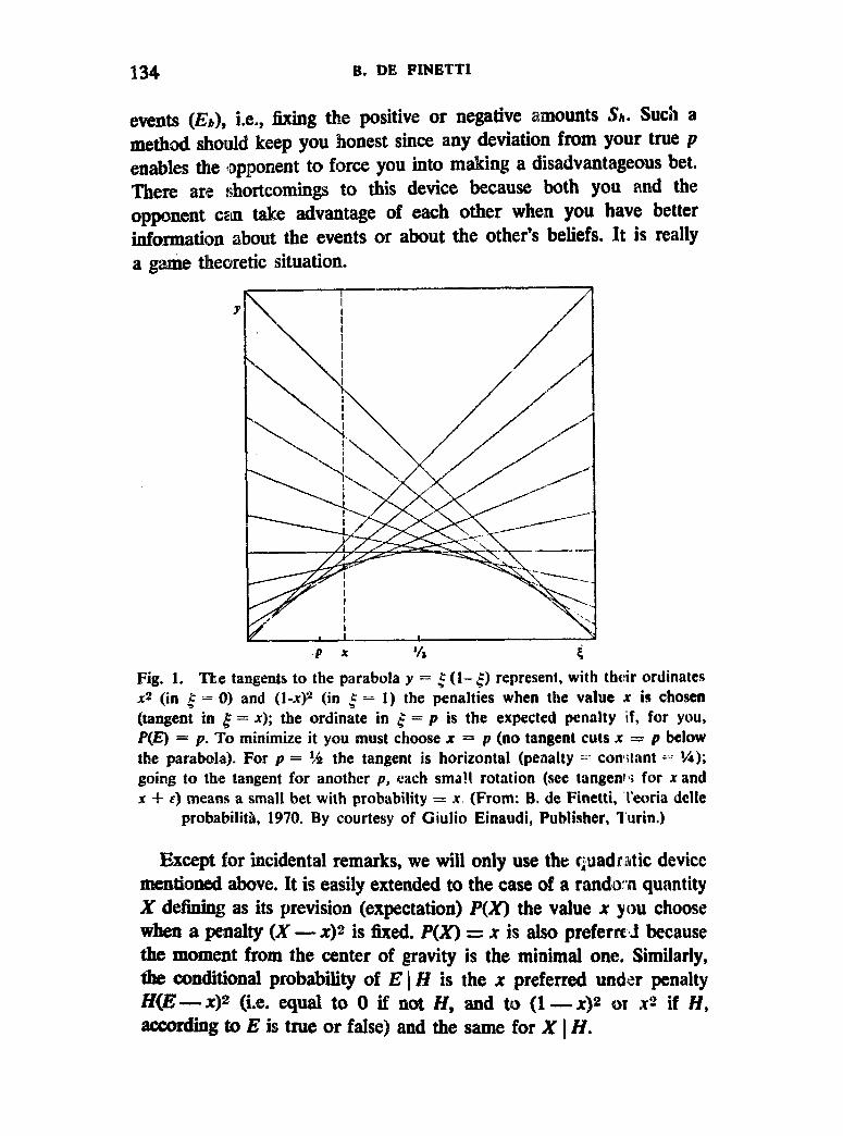
interpretation of the device seems illuminating. For x = 4, the penalty is 8, no matter whether E is true or false; if p > 3, to increase x from 4 to p means t,o seize the opportunity of a continuum of advantageous infmitesimal b&s based on probabilities x from f to p (:and symmetri- cally if p < 3. This is made clear in fig. 1.

Other devices of simillar structure are easily obtained by replacing the parabola in fig. 1 by any other convex function. Devices where several events are considered together (e.g. those of a partition) also may use a global penalty function instead of the sum of penalties associated with each event.

The intervention of an opponent is typical of a different kind of device. Suppose that, on the basis of the betting rates in chosen by you, the opponent is free to impose a bet for or against each of the

134 B. DE PINETTI

eVeEtS (Eh), i.e., fixing the positive or Eegathe amounts Sh. such a method should keep you honest since any deviation from your true p enables the iopponent to force you into making a disadvantageous bet. There are shortcomings to this device because both you and the opponent can take advantage of each other when you have better infomatio~ about the events or about the other’s beliefs. It is really a gtie theoretic situation.

P x ‘/a i

Fig. 1. The tangents to the parabola y = 5 (I- b 2) represent, with their ordinates X* (in 6 = 0) and (l-x)2 (in t = 1) the penalties when the value x is chosen (tangent in l = x); the ordinate in ,$ = p is the expected penalty if, far you, P(E) = p. To minimize it you must choose x = p (no tangent cuts x = p below the parabola). For p = ?4 the tangent is horizontal (penalty =-I coni’lant 2; !4); going to thle tangent for another p, each sma!! rotation (see tangents for x and x + E) means a small bet with probability = x. (From: B, de Finetti, ‘I’eoria dclle

probabilitg, 1970. By courtesy of Giulio Einaudi, Publisher, Turin.)

IExcept for incidental remarks, we will only use the quad.rwtic device mentioned above. It is easily extended to the case of a randoTt quantity X dehing as its prevision (expectation) P(X) the value x you choose when a penalty (X -x)2 is fixed. P(X) = x is also preferre;l because the moment from the center of gravity is the minimal one. Similarly, the WE&~OE~~ probabiity of E 1 H is the x preferred un&:r penalty H(E - x)2 (i.e. equal to 6 if not H, and to (1 - x)2 cur xe if H, according to E is true or false} and the same for X 1 H.


5. RULES OF CONSISTENCY

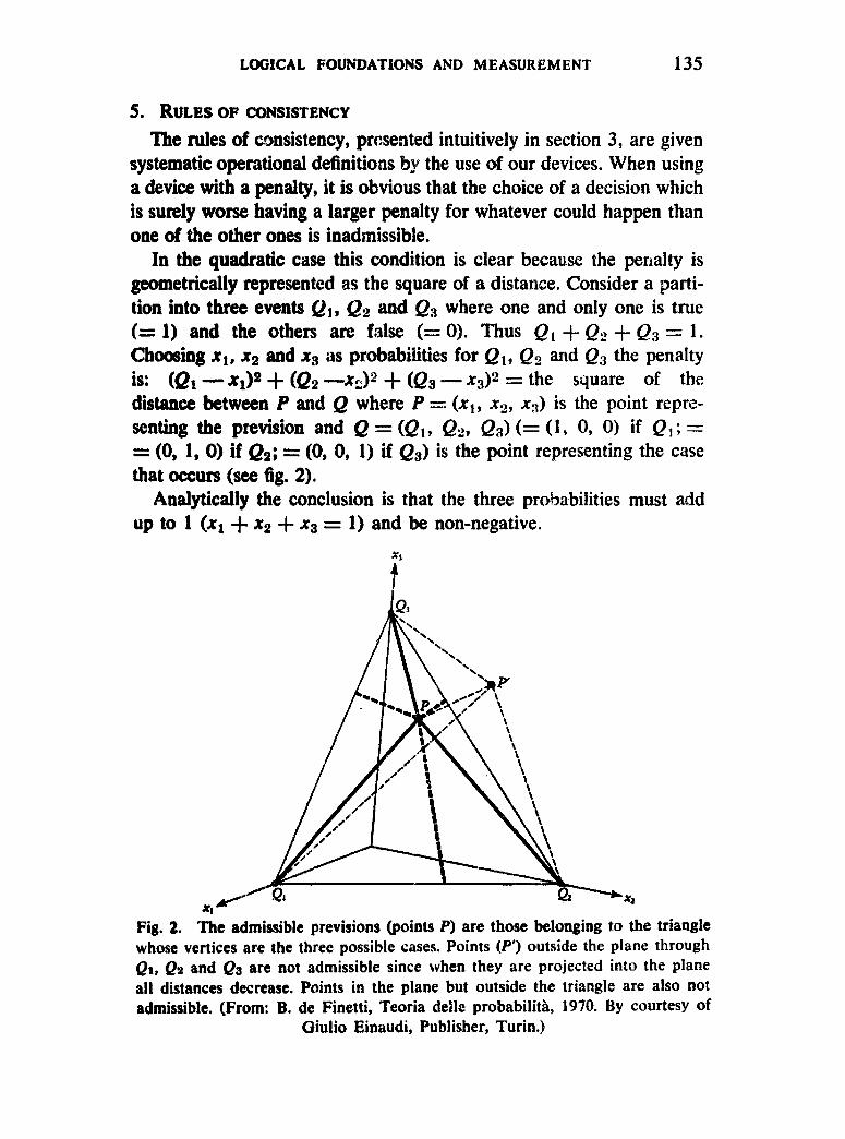
The rules of consistency, presented intuitively in section 3, are given systematic operational definitions by the use of our devices. When using a device with a penalty, it is obvious that the choice of a decision which is surely worse having a larger penalty for whatever could happen than one of ?he other ones is inadmissible.

In the quadratic case this condition is clear because the penalty is geometrically represented as the square of a distance. Consider a partition into three events Q,, Q, and Q3 where one and only one is true (= 1) and the 0th ers are false (=O). Thus Q,+Q,+Q,=l. Choosing xl, x2 and x3 as probabilities for QI, Q, and Q3 the penalty is: (QI - ~$3 + (Q2 --x2)2 + (Q3 - .x3)2 = the square of the distance between P and Q where P = (x1, x2, x3) is the point representing the prevision and Q = (Q,, Qa, Qd (= (1, 0, 0) if 9,; I= = (0, 1, 0) if Q2; = (0, 0, 1) if QY) is the point representing the case that occurs (see fig. 2).

Analytically the conclusion is that the three probabilities must add up to 1 (x1 + x2 + x3 = 1) and be non-negative.

Pig. 2. The admissible previsions (points P) are those belonging to the triangle whose vertices are the three possible cases, Points (P’) outside the plane through QI, QI and Qa are not admissible since when they are projected into the plane all distances decrease. Points in the plane but outside the triangle are also not admissible. (From: B. de Finetti, Teoria delle probabilith, 1970. By courtesy of

Oiulio Einaudi, Publisher, Turin.)

136 B. DE FINETTI

&om&Aly, the same conciusion is reach& the point P must belong tcp the convex hull of the set of possible points. Analytically, it means that previsions must be additive and convex: PCX + Y) =

=WW-WI, inf X S P(X) 5 sup X for all random quantities: In particular for events: O=infE~P(E)“-supE= l,P(.4 v B) 5 P(A) + P(B), with = instead of 5 if they are disjoint (AB = 0), whilst for the arithmetic sum, Y = number of successes, (Y = A + B, or, in general, Y=E&&+... + En) it is always P(Y) = = P(A + B:) = P(A) + P(B), or P(Y) = P(EI) + P(&) $- . . . + + P(En).

With reference to a partition, the conclusion is that all admissible previsions give to the elementary cases non-negative probabilities which add up to one (and their unions to the sum). probabilities (P(AI3) = P(A) P(B 1 A)) may similar geometric representation, here dealing points and a segment instead of from three example (see fig. 3).

The rule for compound also be illustrated by a with distances from two points, as in our initial

w c--

r ----__ ------_____ (1. 1, 1) p”

___-----C--C-

Fig. 3.. Geometric representation for compound probabilities. (From: B. de Fiuetti, Teoria delta probabilith, 1970. By courtesy of Giulio Einaudi, Publisher,

Turin.)


It is instructive to compare the foundations of this approach with the one where an opponent has a role. Admissibility {or consistency, or coherence) means in this case: prevent the opponent from finding an)* opportunity for a Dutch Book.

It is almost evident (even from the preliminary remarks of section 3) that the rules given above are necessary and sufficient for that purpose.

As necessary conditions these conclusions are not at all ne.w: they have been agreed upon by statisticians for years. ‘What is new is to say that they are sufibzt conditions, that no further restrictions need be imposed. In one sense, every one probably could agree with a weaker wording: all consistent previsions are formally admissible, but other reasons (e.g. logical or empirical) may impose further restrictions. Such issues will be considered in section 10.

6. AUXILIARY METHODS

We have now established that the formal rules normally used in probability calculations are also valid, as ronditions of consistency for subjective probabilit.ies. You must obey them, not because of any logical, empirical or metaphysical meaning of probability, but simply to avoid throwing money away; to avoid selling a dollar for less than one dollar. In this spirit we can reconsider the usual procedures for measuring (or, as is often said, defining) probabilities in various situations.

The subjective version of the so-called ‘classical definition’ is but an obvious corollary of additivity: if the N cases of a given partition are, for you, equally probable (or nearly so) each one has, for you, a probability of l/N, and any unian of M of them has a probability of M/N (or nearly so). Symmetries or similarities, both in objective circwmstances and in personal states of uncertainty, may often lead you to such a situation (e.g. in the classical example of drawings, where the N cases do not differ for any significclnt circumstance). But it is for you to judge, in any single instance, whether or not some differen- tiating czcumstances are ‘significant’ which really means (escaping self-deceit) whether or not they influence your beliefs.

TPe ensuing method is useful not only for direct applications (e.g., the drawing of a white ball from an urn, where there are 27 white out of 106, has a probability of 27 % if, in your opinion, it is symmetrical), but also as a general method of comparison. P(E) = 27 %, for whatever E, means that in the scale of drawings with k white balls among

138 B. DE FINETTI

100, your belief about E is nearly the s;ame as for k = 27. This method may help in numerical applications and may add to the first method as equivalent to paying ‘27 for 100 if E’.

An extension is gained by using the property of gensral validity: the sum of the probabilities must equal the expected number of successes. Stated another way: average probability (sum divided by the number of events considered) is equal to expected frequency. This is the rule L9rPI(Eh) = P(Y) (see section 5) or (1 /N) XnP(Eh) = P(Y/N). If Y is known (certain) the word ‘expected’ may be dropped. In partrcular Y = 1 (surely) is the preceding case of a partition. If the En are, for you, equally probable, the word ‘average’ may be dropped (and ‘sum of . /I .’ is ‘N times the . . .‘).

There are many cases where the frequency is known (e.g., it is kaown in advance how many among all candidates will be selected; just after the votes are counted, it is known how many of a given party are etected but not which ones) and in many more cases you have some beliefs about the frequency (e.g., of candidates passing a given examination, or of rainy days next year). This is an aid in evaluating the probabilities of the single events (success of each of the candidates or rain on each one of the 365 days) when taking into account the differences that we know (ability of each candidate or seasonal weather changes), or, if any relevant information is missing by taking the expected value of the frequency as the estimate of the probability of each one of the events.

The expectation of a frequency in the future is often based on the observed frequency of similar events in the past. This fact is outside th.e domain of present considerations.

For tbe moment it must be accepted as a ‘faith in stability’, it can be better understood and justified later (see section 11).

7. THE USEFULNESS OF PHOBABILlSTIC THINKING AND BEHAVIOR

We are always living and dealing in conditions of uncertainty. If probabilistic thinking is to be the guide in facing uncertainty, it is essential that we learn how to do it ‘cmrecfly’. To know the rules of probability and to be acquainted with their practical application is to free us from the danger of inconsistency. But someone could object, in order to do this ‘correctly’, should we not also learn how to evaluate the probabiities ‘correctly’ by some ‘objectively’ valid procedure?


That aim is justified, but the solution is misleading; there is no better advice than to carefully weigh all information and every circumstance. So called objective methods are only rough rules of thumb, suggesting that only the most schematic data be taken into account in the most schematic manner. That is not necessarily bad, but not necessarily good either. Maybe your immediate beliefs are not weighed in the mind. But often your belief is better founded than any other, particularly if you are in the habit of considering all faces of a situation, not only the most obvious ones.

But what does it mean if no objective criteria of comparison exist? The answer is again a question: since no objective criteria exist, does one refrain from subjectively judging the subjective ways of weighing evidence for his own thinking and for his own behavior? Does one refrain from comparing them with each other and comparing their results? Does one refrain from learning from experience? WC must never complain that we could not foresee wh.at was going to happen for we are not prophets. Rather, we must simply consider, in light of what happened, whether a better analysis of the prospects could have been made based on the information then available. The aims of theory and of practice all require the use of careful subjective reasoning as a necessary substitute for objective criteria which are non-existent.

To summarize, it is important to: (a) develop the ability to weigh degrees of probability;

(b) become aware of consistency and learn to obey it instinctively;

(c) make re-evaluations following new information or new experiences;

(d) try to evaluate different probability assesso:rs;

(e) develop methods based on the evaluation of subjective probabilities in many practical fields;

(f) improve behavior during uncertainty by means of probabilistic thinking and the concept of utility;

(g) find the ide:as and language that will make this topic as simple and easy as it really is. The present language is totally inadequate because, as Jeffreys observed: ‘ordinary language has been created by realists, and mostly very naive ones . . . We have enormous possibilities of describing the inferred properties of objects, but very meagre ones of describing the directly known ones of sensation . . . The idealist must either do his best with realist language or make a new one, and not much has been done in the latter direction’ (JEFFREYS, 1961, b. 423).

140 B. DE FINETTI

8. SCORING RULES AND THE EVALUATION OF ASSEssfXs

Does it mabe sense to speak of ‘good probability appraisers’? This is the question I posed in the title of a first short descflption of an

experiment (DB FINETTI, 1962) and it seems necessary to say something about the subject here in the course of further developing the points of section 7.

until now the property needed in order for a device (i.e. for a scoring rule) to be suitable for eliciting probabilities was only that of ‘keeping

the assessor honest’. However it is explicitly felt that an assessor getting

a 1~ penalty in the long run is better. In fact, if we suppose for a

moment that ‘objective probabilities’ exist for events in the experiment, assessors giving the correct values of the objective probability would get the best expected score and thus in the long run, the best attained score.

But the state of affairs is not so simple. Several questions have been raised by WINKLER (1969) with reference to ROBERTS ( 19653. See also

STAHL VON HOLSTEIN (1969), DE FINETTI (1970) and DE FINETW and SAVAGE (1962). The situation is growing more complex rather than approaching a clarification. Now there are several different points of view on scoring rules.

One oversimplified version is to consider a fixed scoring rule and to assume that we know only the scores attained by a number of assessors on a large set of items (items or facts with several outcomes). One oversimplified conclusion seems legitimate: the score in the past is a good basis for future scores (in similar experiments); if 1 had to adopt the predictions of one of the assessors I should choose to follow the one with the best score. But, if the best person attained the best possible score (that he has dared to give 100 % probability to a single outcome fur each item and has always been correct) 1 probably would consider him a fool who has been strangely lucky until now and who would be quite unreliable in the future,

An extremely complex version (in a Baycsian sense) would be knowing how my forecasts of today would be intluenced by the knowledge of the forecasts of one of the other assessors, taking into account his past forecasts for each item and its outcome.

It is easy to imagine many intermediate versions which would ~r=sflond to diflEerent purposes, A rather practical one consists of giving different weights as penalties to ‘errors’ of different importance, In football, for example, the distance ‘between winning and losing is not


a constant: there is a difference between losing closely or being over- whelmed. In the same way the distance between a victory and a draw, or a defeat and a draw, is not constant.

Tn general one may give a constant penalty on the prediction of h,

if the observed event is k $ h, or give the penalty a weight proportional to (h- k 1. This is a wide field which deserves attention both of mathematicians and psychologists.

9. PSYCHOLOGICAL ANALYSIS OF ASSESSORS

The several versions of evaluations of assessors given in section 8 show that simply ordering them by a score hardly gives a satisfactory evaluation. A more interesting and useful technique must include the characteristic features of their evaluations and distinguish all possible relevant aspects (or at least, all of those that we can think of and investigate). For example WC can mention: (1) degree of competence or care in forecasts concerning different subject mat&s, epochs or regions; (2) optimistic or pessimistic attitudes: e.g. the tendency to ovr’r- estimate favorable or desired outcomes (wishful thinking) or the opposite; (3) degree of influence of the most recent facts (e.g. to put much weight on recent performance of a football team rather than on its record over several years); (4) degree of deviation from statistical standards, according to spectic knowledge of each item (e.g. from mortality r,ltes based on personal characteristics; from the average - 50 %, 30 %, 20 % for winning, tying, losing in football - based on the qualities of the teams involved in a particular match); (5) stability or flexibility (evolutionary or oscillating) of opinions without a change in the available informarion, by thinking about or by the influence of another’s opinions. A distinction must be made between the cases when the subject remembers his past answers and is conscious of his change (or lack of change) and when he answers afresh without conscious connection with his past answers; (6) conscious or unconscious adaptation of the opinion td standard patterns of statistical theory and practice; (7) the same, in the very important case of adaptation to changing information following either the true Bayesian framework or some empirical substitute;

142 B. DE FIHETTI

(8) the same, with reference to the mental model where the subjective pr&&iliQ is viewed as ‘an estimate of an unknown but supposedly existing ob@ctive probability’ (which may be either lo&d or physical). One should investigate why some individuals believe that the one, the other or both “kinds of probability ‘exist’ and what they mean by the word ‘exist’. Other questions arise if we regard the assessors collec- tively rather than individually. It is interesting e.g.: (9) to study the distribution of probabilities given to the same event by d&rent individuals of a group or of subgroups; (10) to compare the individual scores with the score of a fictitious player who adopts as his subjective probabilities for each event the average probability given to this event by a group or subgroup. It often happens that this fictitious player is near the top of the performance range. It is CE if the individual opinions were estimates of an ‘objective probability’ given by the average. The use of ‘as if’ does not imply any meaningful interpretation.

10. BELIEFS ABOUT REALiTIES VS. BELIEFS ABOUT FICTIONS

ket US expand 8 from section 9 and try to answer the question put forth at the beginning: how can we reconcile the subjectivistic basis of pr&&ility theory given here with the objectivistic point .of view? Objectivists believe that there exists for some events something called ‘ob,icctive probability’. Perhaps some believe only in ‘logical’ and some only in ‘physical’ probabilities and others in both, but this makes no difference. When I am engaged in Gticizing their ideas I am obliged to prctcnd that they are intelligible to me. Here the situation is much better: I may admit outright the existence of a meaning which is intelligible for some people, disregarding the fact that 1 am unable or do not care to understand it.

An objectivist. admits that objective probabilities may exist which are either known or unknown to him. If he knows some objective probabfities, they are also his subjective probabilities (as seen in section 6) and (there is nothing more to be added. Most objcctivists also seem inclined to deal with unknown probabilities, often in a way which enables them to follow (in a disguised form) subjectivistic reasonings.

Subjective probabilities may be considered by objectivists as csti- mates of objective ones (whenever they exist). It would be reasonable, to avoid exceptions and confusing definitions, to consider also the case


of “known’ objective probability as a limiting case where one is almost sure that the unknowable objective probability is close ,to his subjective probability.

This way, there is practically no difference with the position of Good, a subjectivist who considers sane the use of such a mental model. It would be a totally innocuous model if used in the simple case of single probabilitie s. Then it would consist of imagining a subjective probability as the mean of a distribution of the possible values of something called ‘objective probability’. But the procedure becomes illuminating when a whole process is considered as an average, here better said a mixture of simple processes.

The fundamental example is the one of ‘Bernoulli processes with unknown probability’ that are ‘mixtures of Bernoulli processes’: <.his last wording, with no more reference to unknown objective probabilities is exactly the description of the ‘exchangeable process’ by means of their most significant mathematical property, in a way that a subjectivist would approve.

11. ti FUNDAMENTAL EXAMPLE

The missing link in the explanation (section 6) of why e::.pccted future frequencies should be guessed according to past observed frequencies (and one that embraces the whole problem of inference) is met here in a form where the subjectivistic and the objectivistic interpretations are strictly connected.

The ‘mixture’ property, interpreted as expressing a prob:lbility distribution for the unknown probability, causes us to guess this unknown probability according to the observed frequency that is In- formative for this purpose regardless of whether the proper Brlyesian method is followed or ‘ad hoc’ rules are applied.

The exchangeability property leads directly to the Bayesian rc’nults, and does not require nor justify the use of me&physical concepts like unknown probability. Exchangeability is a realistic concept not in- volving an infinity of possible trials because it simply says that the probability of a combination of a finite number of events of the process remains unchanged no matter how such events ure dmsr~?r and permuted, 1

2 A simpler (but perhaps less expressive) formulation is the follouing: pro-

ducts of PJ among the events of the process hilve ali the same prolxtbility dcpend-

ing only on II, not nn the rr-tuple chosen,

144 B. DE FINETTI

~~~ exmple should clarify in what sense the concept of unknOWn

pr&&aity h the considered model must be seen as fictitious and misleading. It is well known that the processes of Bayes-Laplace and Pblya are identical as probabilistic models although very different in the way they are produced. Bayes-Laplace process is a Bernoulli process.

h the drawing of balls (with replacement) from an urn containing white and black balls in an unknown proportion, the probability diitribution of this proportion is uniform over the interval (0,l). 3

A Pblya process (contagious probabilities) consists in drawing balls from an urn containing, in the beginning, two balls, one white and one black, and where after each draw, not only is the ball drawn replaced, but also another one of the same color is added. After N = W + B drawings (W z number of white, B = number of black) there are N + 2 balls (W + I) white and (B + 1) black; the probability of white on the next trial is (W + l)/(N + 2). But, surprisingly enough, this is the same that happens in ,the Bayes-Laplace model: that is the famous Laplace succession rule.

What is the lesson? In the Bayes-Laplace version it is correct to call ‘unknown probability’ the ‘uaknown proportion* (which has a real exis’tence). The wording would be: ‘the probability of‘ each trial conditional to the knowledge of the unknown proportion and given the fact that my subjective opinion agrees with the standard assumption that the drawings are stochastically independent and that all the balls have equal probability.’

In the P6lya version it is formally possible to think of a fictitious urn of B~ytr~-La#~z type existing in some supposed world of Platonic idea, governing the happenings observable in our world of poor appearances and. of copies or from ‘true knowledge”. But that, outside Platonism, is obviously a pointless fiction.

In conclusion: the recourse to concepts like ‘&je&e unknown probability’ in a problem is neither justified nor ~eful for intrinsic reasons. It may correspond to something realistic under particular

facml feamres, not of a proba ilistic model, but of a specific device.

3 We have an approximate model by making the total number of balls, N, very high, and making the N + 1 possible values of the number af white balls equatly probable (l/(N + 1) ). Only a contimrous model could be exact (like roulette where the proportion of white sectors has a uniform distribution).


But to speak of ‘unknown probability’ is always misleading unless the possible true interpretation underlying it is clearly and carefully explained.

REFERENCES

DE FINETTI, B., 1962. Does it make sense to speak of ‘good probability appraisers”? In: I. %. Good (cd.), The scientist speculates: An anthology of partly-baked ideas. New York: Basic Books.

I 1970. Probabilitb di una teoria e probabilith dei fatti. Contribution to a meeting in honor of G. Pompilj, Rome 1970, to be published. and L. 3. SAT&GE, 1962. Sul modo di scegliere le probabilitj, iniziali. Bibl. d. Metron, Ser. C’ , Vol. 1, Rome.

JEFFREYS, H., 1961. Theory of probability Third edition. Oxford: Clarendm Press.

ROBERTS, H. V., 1965. Probabilistic prediction. J. Amer. statist. Ass. 60, 50-62. STABL VON HOLSTFQN, C.-A. S., 1970. Some problems in the practical application

of Bayesian decision theory. In: Behavioral approaches to modern management. Gothenburg: The Graduate School of Economics and Business Administration, in press.

WZNUER, R. L., 1969. Scoring rules and the evaluation of probability assessors. J. Amer. statist. Ass. 64, 1073-1078.

logical foundations and measurement of subjective probability

Documents