logic and distributed control system - biher · computer control system expand present control...

Computer Networking

Software-Defined Networking (SDN)

Software-Defined Networking

• Motivation• Enterprise network management• Scalable SDN

• Readings:• A Clean Slate 4D Approach to Network Control and

Management• Onix: A Distributed Control Platform for Large-scale

Production Networks• Optional reading

• Ethane: Taking Control of the Enterprise



• Readings:• A Clean Slate 4D Approach to Network Control andManagement• Onix: A Distributed Control Platform for Large-scale



4D: Motivation

• Network management is difficult!

• Operators goals should be implemented as “workarounds”

• Observation: current Internet architecture bundles control logic and packet handling (e.g., OSPF)

• Challenge: how to systematically enforce various, increasingly complex high-level goals?

Design choices

• Incremental deployment• Advantage: easier to implement• Disadvantage: point solution?

• 4D advocates a clean-slate approach• Build control plane/network management from the

ground up• Constraint: no change of packet formats

• Insight: Decouple the control and data planes

Example 1: Front- Office Data Center ACL

Example 2: Spurious Routing

Management today

• Data plane• Packet forwarding mechanisms

• Control plane• Routing protocols • Distributed

• Management plane• Has to reverse engineer what the control plane• Work around rather than work with!

Driving principles

• Network-level objectives• High-level, not after-the-fact

• Network-wide views• Measurement/monitoring/diagnosis

• Direct control• No more “reverse engineering” or “inversion”• Direct configuration

4D Architecture

• Decision plane• routing, access control, load balancing, …

• Dissemination plane• control information through an independent channel

from data

• Discovery plane• discover net. elements and create a logical net. map

• Data plane• handle individual packets given state by decision plane

(e.g., forwarding tables, load balancing schemes,…)

Advantages of 4D Architecture

• Separate networking logic from distributed systems issues

• Higher robustness

• Better security

• Accommodating heterogeneity

• Enabling of innovation and network evolution

Challenges for 4D

• Complexity

• Stability failures

• Scalability problems

• Response time

• Security vulnerabilities

Research Agendas

• Decision plane

• Dissemination plane

• Discovery plane

• Data plane

Research Agendas

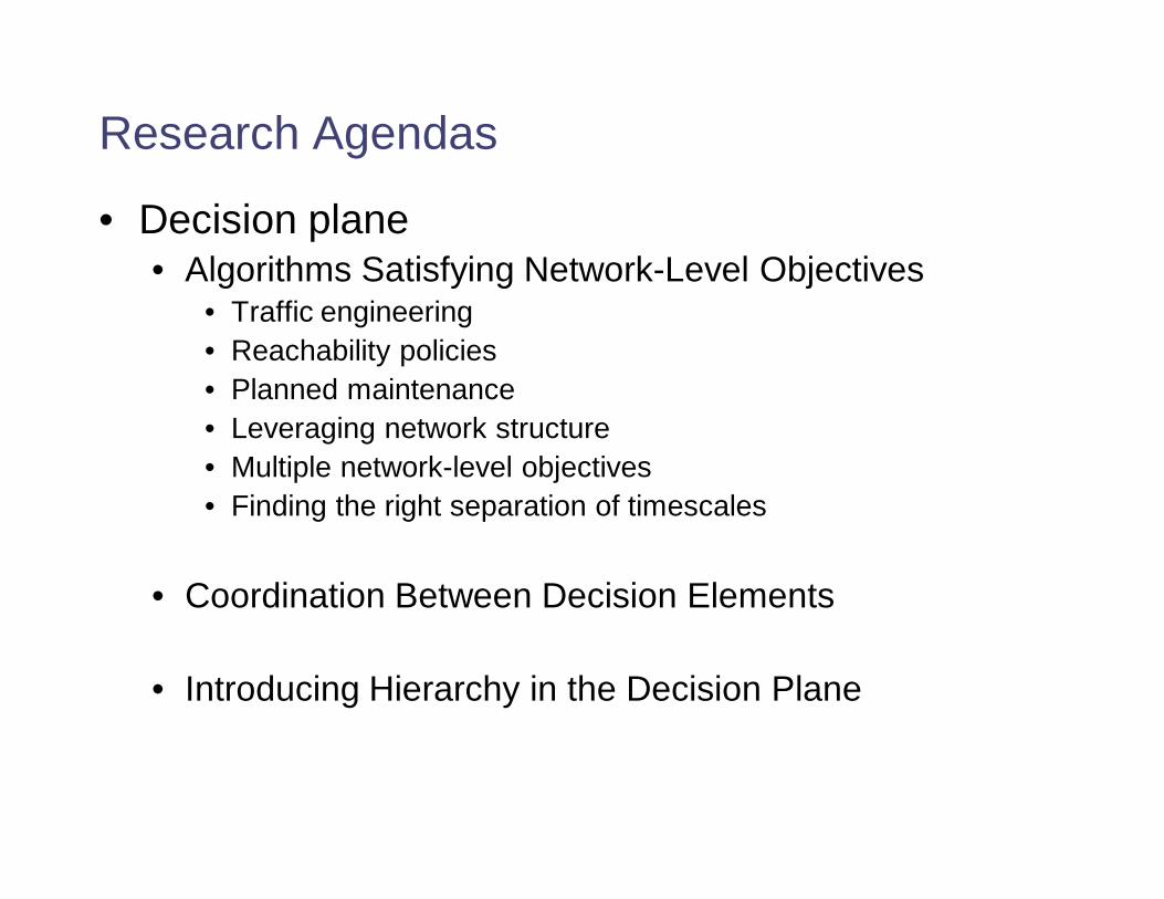
• Decision plane• Algorithms Satisfying Network-Level Objectives

• Traffic engineering• Reachability policies• Planned maintenance• Leveraging network structure• Multiple network-level objectives• Finding the right separation of timescales

• Coordination Between Decision Elements

• Introducing Hierarchy in the Decision Plane

Research Agendas


• Coordination Between Decision Elements• Distributed election algorithms• Independent DEs

• Introducing Hierarchy in the Decision Plane

Research Agendas


• Coordination Between Decision Elements

• Introducing Hierarchy in the Decision Plane• Large network managed by a single institution• Multiple networks managed by different institutions

Research Agendas

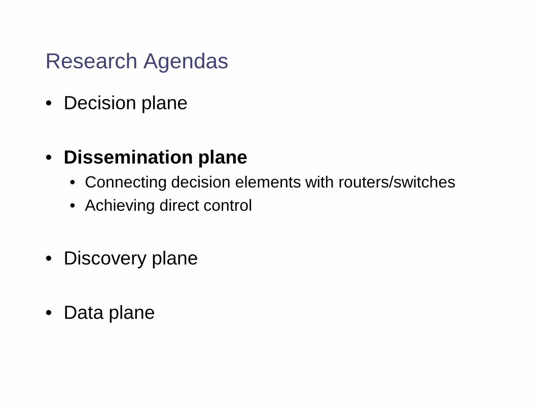
• Decision plane

• Dissemination plane• Connecting decision elements with routers/switches• Achieving direct control

• Discovery plane

• Data plane

Research Agendas

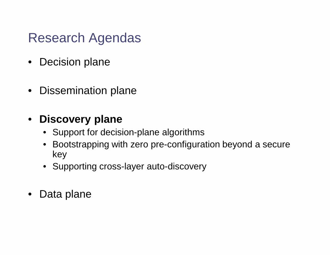
• Decision plane


• Discovery plane• Support for decision-plane algorithms• Bootstrapping with zero pre-configuration beyond a secure

key• Supporting cross-layer auto-discovery

• Data plane

Research Agendas

• Decision plane


• Discovery plane

• Data plane• Packet-forwarding paradigms• Advanced data-plane features

Where are we?

Controller

Config Config4D

(vision)

Where are we?

Controller

Config Config

OpenFlow

Where are we?

Controller

Config Config

Ethane(concreteexample)

Where are we?

Controller

Config Config

E.g., ONIX




Management• Onix: A Distributed Control Platform for Large-scale



Motivation

• Enterprise configuration• Error prone: 60% of failures due to human error• Expensive: 80% of IT budget spent on maintenance

and operations

• Existing solutions• Place middleboxes at chokepoints• Retrofit via Ethernet/IP mechanisms

Driving question

• Make enterprises more manageable

• What’s good about enterprises• Security policies are critical• Already somewhat centralized

Three principles in Ethane

• Descriptive/declarative policies• Tie it to names not locations/addresses

• Packet paths determined explicitly by policy

• Binding between packet and origin• No spoofing• Accountability

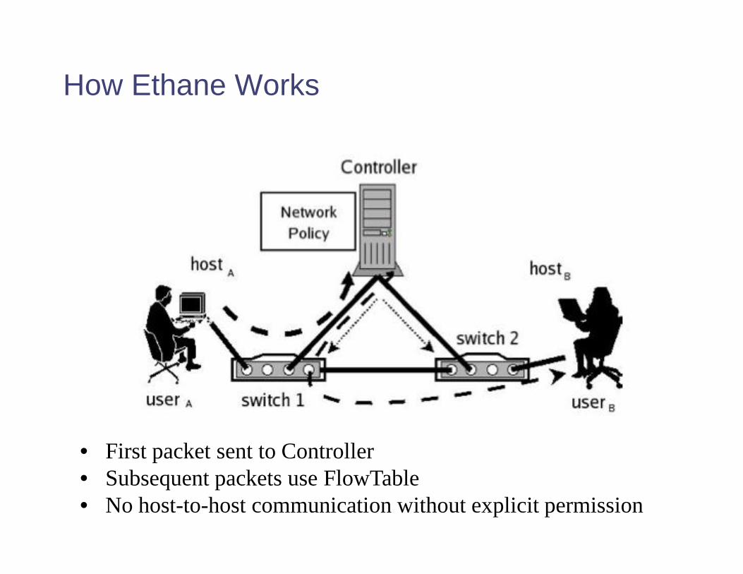
How Ethane Works

• First packet sent to Controller• Subsequent packets use FlowTable• No host-to-host communication without explicit permission

Ethane in use

1. Registration• explicit registration of users, hosts, and switches

2. Bootstrapping• spanning tree

3. Authentication• controller authenticates the host and assigns IP• user authenticates through a web form

4. Flow set up

5. Forwarding

Controller Design Components

• Explicit per-flow way-pointing

Switch Design

• Flow Table

• Local switch manager

• Secure channel to controller

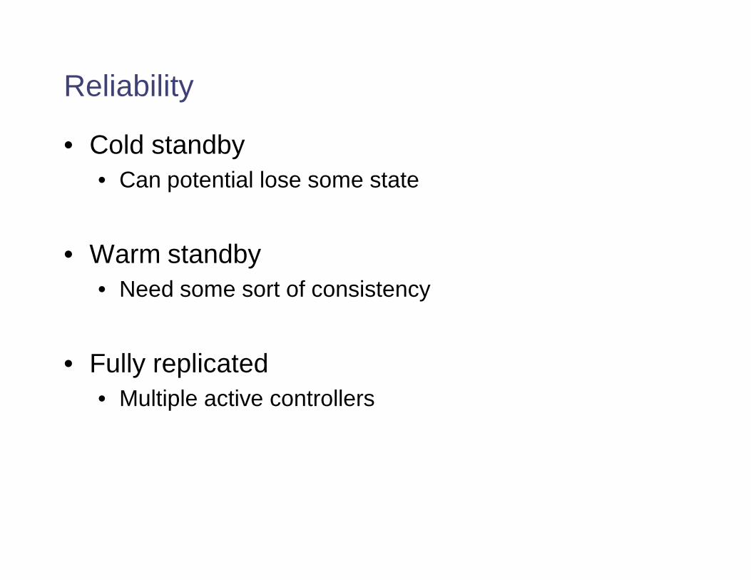
Reliability

• Cold standby• Can potential lose some state

• Warm standby• Need some sort of consistency

• Fully replicated• Multiple active controllers

Policy Language

• Common tasks expressed as predicates

• Allow, deny, waypoint

• Interpret vs compile

Policy Language

Potential resource concerns

• Controller “DDoS”

• Controller scalability

Evaluation

• Mostly “feasibility”

• Trace-driven evaluations

• Failure emulation

• Scalability of request rate

• End-to-end performance

Ethane Prototype

• 300 hosts in CS department at Stanford

• Multiple “switches”• Wireless access point, linux, netfpga

• Controller• Standard linux PC • Linux PC (1.6GHz Celeron CPU and 512MB of DRAM)

• Controller handles 10,000 flows per second

Experiences

• Once deployed, easy to manage

• Add new switches, users is easy

• Journaling helps debugging

• Adding new features is easy

Advantages of Ethane

• Switches• Dumb• No complex distributed protocol• Focus purely on forwarding• Save forwarding rule space (try to keep only “active”

flows)

Comments on Design

• Common vs worst case design?

• Latency, scalability




Management• Onix: A Distributed Control Platform for Large-

scale Production Networks• Optional reading


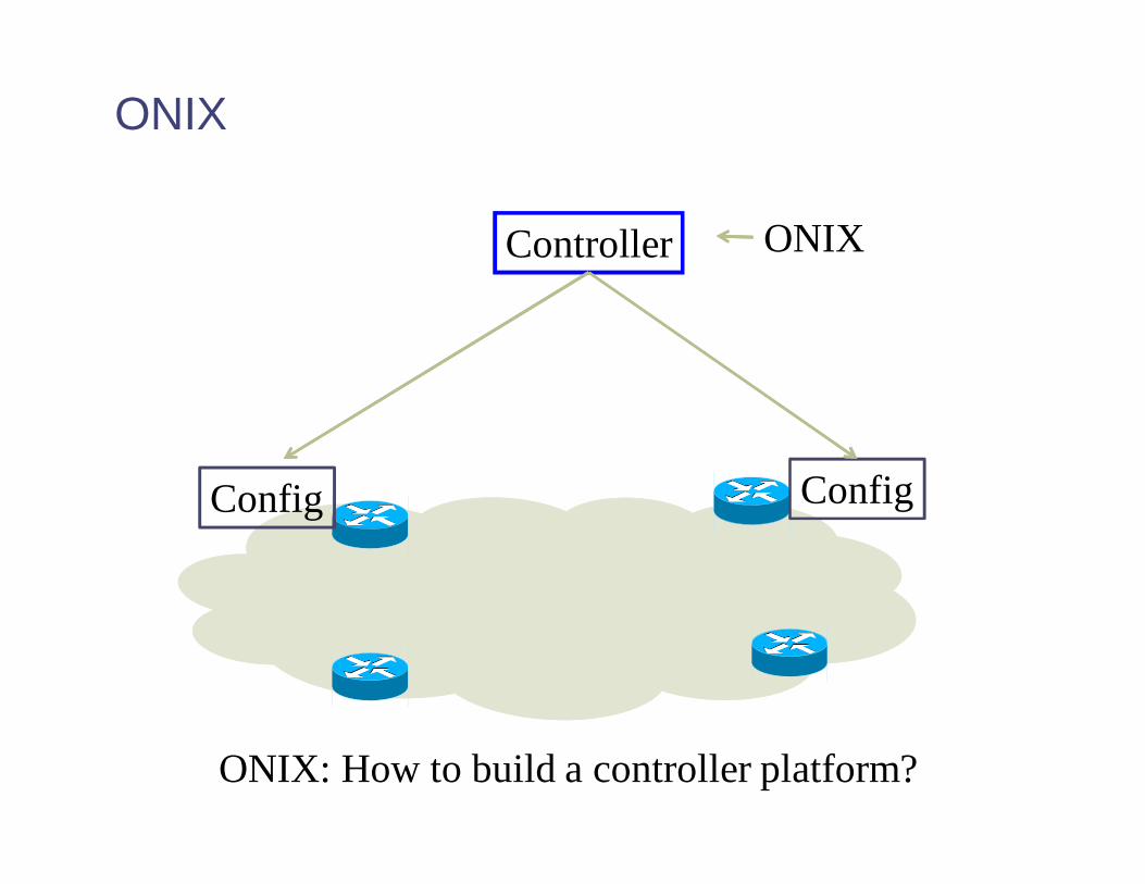
ONIX

Controller

Config Config

ONIX: How to build a controller platform?

ONIX

What are the key challenges?

• Usability

• Performance

• Flexibility

• Scalability

• Reliability/availability

ONIX Design Decisions

• “Data-centric” API

• Treat all networking actions as data actions• Read• Alter• Register for changes in network state

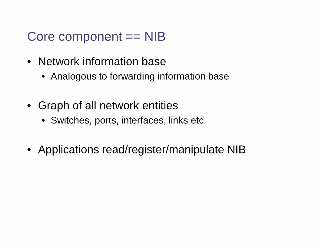
Core component == NIB

• Network information base• Analogous to forwarding information base

• Graph of all network entities• Switches, ports, interfaces, links etc

• Applications read/register/manipulate NIB

Core component == NIB

• NIB is a collection network entities

• Each entity is a key-value pair

Default network entity classes

ONIX NIB APIs

Functions provided by the ONIX NIB API

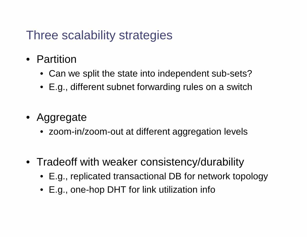
Three scalability strategies

• Partition• Can we split the state into independent sub-sets?• E.g., different subnet forwarding rules on a switch

• Aggregate• zoom-in/zoom-out at different aggregation levels

• Tradeoff with weaker consistency/durability• E.g., replicated transactional DB for network topology• E.g., one-hop DHT for link utilization info

Two types of datastores

• DHT with weak eventual consistency• Used for “high” churn events• Frequent updates

• Transactional store with strong guarantees• Used for “low” churn events• E.g., network policy

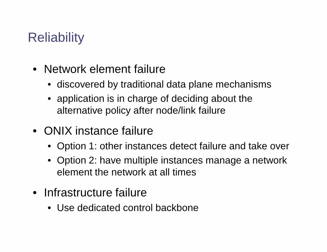
Reliability

• Network element failure• discovered by traditional data plane mechanisms• application is in charge of deciding about the

alternative policy after node/link failure

• ONIX instance failure• Option 1: other instances detect failure and take over• Option 2: have multiple instances manage a network

element the network at all times

• Infrastructure failure• Use dedicated control backbone

Killer apps for ONIX

• Why did VMWare bought Nicira maybe?

• DVS

• Multi-tenant virtualization

Lingering questions

• flexibility

• Performance bottlenecks

• Consistency/conflicts

Summary

• 4D: An extreme design point

• Ethane: End-to-end enterprise network management

• ONIX: A distributed control platform

Next Lecture

• Network verification• Readings:

• HSA: Read in full• NOD: Read intro• Veriflow: Optional reading

UNIT- II

PLC AND ITS APPLICATION

Introduction

• PLC(Programmable Logic Controller)

• Advantages of PLC

• Programming--- Ladder diagram

• PLC in batch processing & others

• Current trends in the industry

PLC(PROGRAMMABLE LOGIC CONTROLLERS)

1. Replaces relays as logic elements.

2. Software oriented.

3. Fixed number of input-outputs/PLC .

4. Programmable.

5. Each I/O can be used as many times as necessary.

6. Downloaded from PC by a cable by the programming port .

SCAN PROCESS OF A PLCSteps in PLC scan process• I/P processing• Program processing• O/p processing

Advantages Of PLC:

1. Flexible2. Cost effective .3. Greater Computational abilities.4. Trouble shooting easier.5. Reduce downtime.6. Reliable.

PLC Programming

Ladder Programming has

•Hot rail

•Neutral line

•Rungs

•Input

•Output

Ladder programming is mostly used

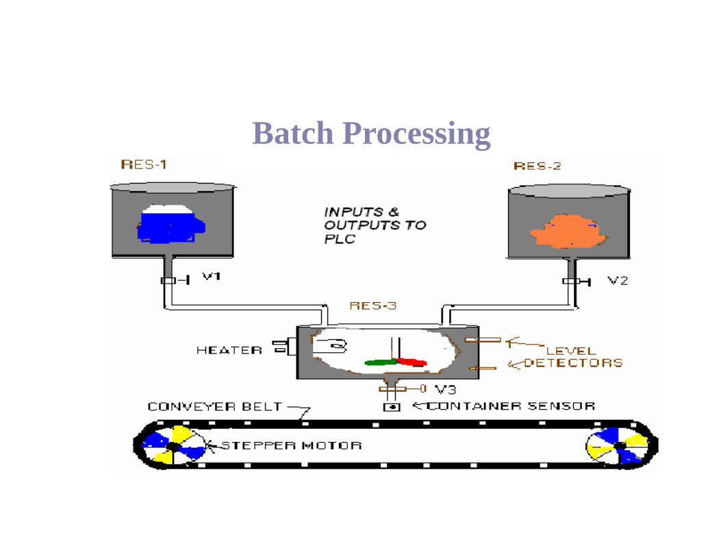
Batch Processing

Ladder Diagram For Batch Processing(VALVE1)

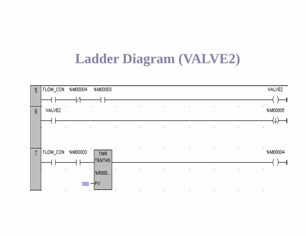
Ladder Diagram (VALVE2)

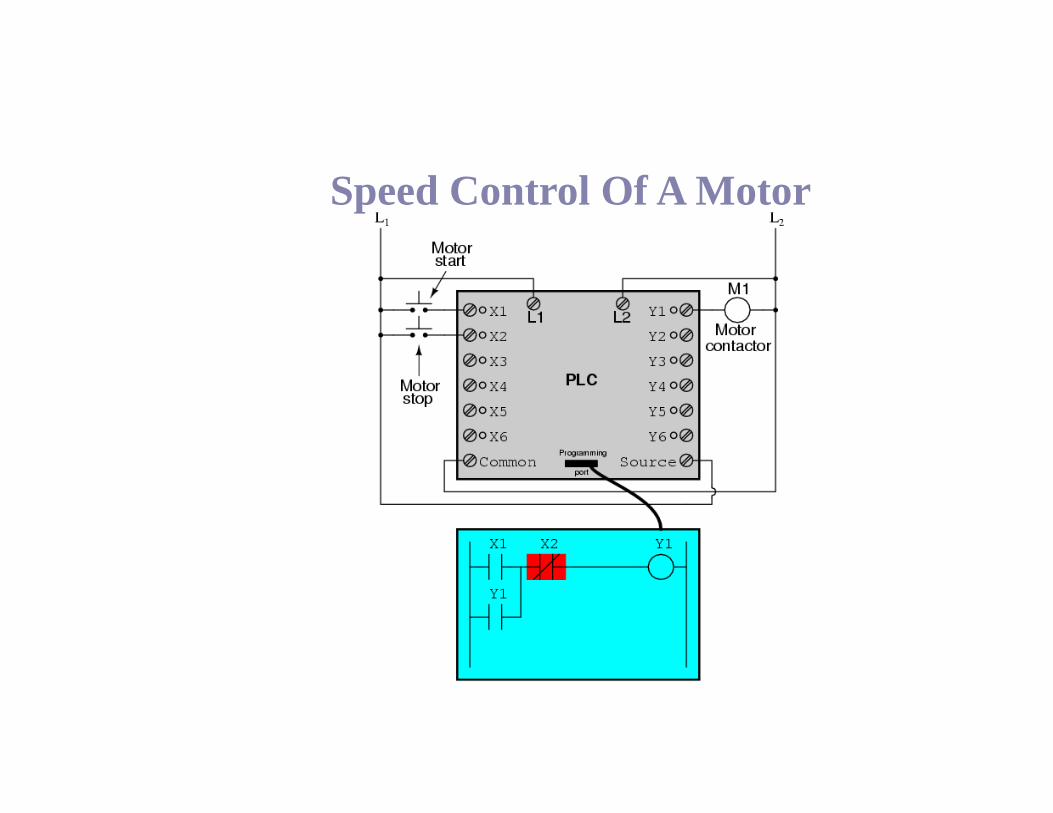
Speed Control Of A Motor

Applications Of PLC1. Petrochemical industry --crude separation etc..

2. Steel industry-- smelter operations, blast furnace, temperature monitoring etc.

3. Power generation -- boiler control from water injection, temperature, fuel, steam flow monitoring etc.

4. Process industries --air flow control, controlling air-fuel ratios etc.

5. Chemical industries-- proportion of chemicals .

6. Nuclear power generation plants .

7. Home automation .

8. PLCs in all phases of automated industrializations.

GEFANUCInputs—14Outputs—10Software used—Versapro (Windows gui)Power supply—24v

MESSUNG

Inputs—8Outputs—6Software used—Doxmini (dos)Power supply—24v

Different PLCs

• “Smart" PLCs microprocessors memory.

• Multitasking.

• Multiaxis control with sophisticated vision systems .

• Hardened programmers Online & offline software development

• Menu-driven software and concurrent operating systems.

Current Trends in the Industry

• Hence we see that PLC are widely used in industries.

• PLCs have been gaining popularity on the factory floor and willremain predominant for some time to come.

• Future of advanced automation.

• Better control and management achieved.

Conclusion

UNIT IIICOMPUTER CONTROLLED SYSTEMS

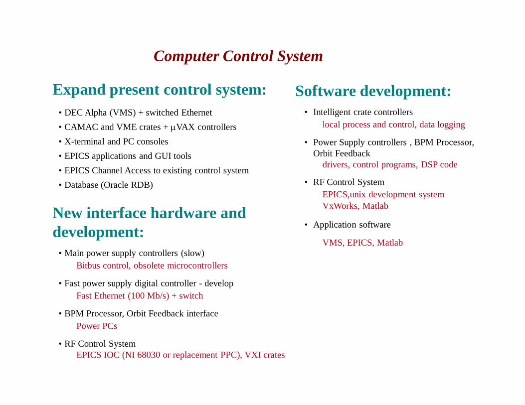
Computer Control System

Expand present control system: • DEC Alpha (VMS) + switched Ethernet• CAMAC and VME crates + mVAX controllers• X-terminal and PC consoles• EPICS applications and GUI tools• EPICS Channel Access to existing control system• Database (Oracle RDB)

New interface hardware and development:

• Main power supply controllers (slow)Bitbus control, obsolete microcontrollers

• Fast power supply digital controller - developFast Ethernet (100 Mb/s) + switch

• BPM Processor, Orbit Feedback interfacePower PCs

• RF Control SystemEPICS IOC (NI 68030 or replacement PPC), VXI crates

Software development:• Intelligent crate controllers

local process and control, data logging

• Power Supply controllers , BPM Processor, Orbit Feedback

drivers, control programs, DSP code

• RF Control SystemEPICS,unix development systemVxWorks, Matlab

• Application software

VMS, EPICS, Matlab

Orbit Control with Matlab and EPICS Channel Access

Matlab-based Accelerator Toolbox and Simulator

H-V coupling error analysis

VME Crates and CPUs

VGM5 VME Dual PPCG4/G3 CPU Board (Synergy)

Dual or single CPUs in a single slot solutionAdvanced PowerPC G4/G3 architecture300-466 MHz CPU speedBackside L2 cache 1 or 2 MB per CPUPØ-PCI(TM) secondary data bus, ~264 MB/s16-512 MB high-speed SDRAMUp to 9 MB FlashSupports industry-standard PMC I/OAutosensing 10/100Base-TX EthernetTwo serial ports standard; SCSI option4-digit clock/calendar chip is Y2K compliantSupports VxWorks, LinuxSupports RACEway with PXB2 PMC moduleVME64x supportVME Speedway doubles non-block transfer rateConformal coating option

VME Crates (Wiener)21 slots, 6U VME cards3U space for fan tray and plenum chamber Card guides and ejector rails IEEE 1101.10Monolithic backplane VME64x or VIPA Microprocessor controlled fan-tray unit UEL

6020 with high efficient DC-fans (3 ea.),alphanumeric display, variable speed fan

Temperature control, front or bottom air inlet Up to 8 temperature sensors in bin area with

network option for remote monitoring andcontrol (CAN-bus)

Remote CPU reset capabilityUsed at SLAC, BNL, CERN, BESSY, etc.

Beam Monitoring and Feedback Systems

New for SPEAR 3:

• BPM Processing System

• Orbit Feedback System

• DCCT

• Scraper Controls

• Tune Monitor

• Synchrotron Light Monitor

• Quadrupole Modulation System

From SPEAR 2:

•Upgraded injection monitors

•Longitudinal Bunch Phase Monitor

•Transverse Bunch Phase Monitor

Central BPM and Orbit FeedbackStation (VME) - Bldg. 117

Corrector Power Supply RacksBldg. 118

Fast Ethernet100 Mb/s

LO + IF Clk

Sync

Ctrl (>12 Mb/s)

Ethernet Inject trig fRF = 476.300 MHz

LO+IF Clk out

LO/ IF ClkGen

SPEARControl

Computer

SPEAR 3 BPM and Orbit Feedback System rev. 5/24/00

8 Hcorrs

8 Hcorrs

8 Hcorrs

Ctrl

Ctrl

Ctrl

8 Vcorrs

8 Vcorrs

8 Vcorrs

Ctrl

Ctrl

Ctrl

8 Hcorrs

8 Hcorrs

8 Hcorrs

Ctrl

Ctrl

Ctrl

8 Vcorrs

8 Vcorrs

8 Vcorrs

Ctrl

Ctrl

Ctrl

6 Hcorrs

6 Vcorrs

spare/misc.

Ctrl

Ctrl

Ctrl

BPM 1 BPM 24

Remote 24-BPMProcessing

Station

Quad 1

BPM 48BPM 17BPM 25


Station

Quad 2

BPM 72BPM 49


Station

Quad 3

BPM 73 BPM 96


Station

Quad 4

Cra

te C

trl(P

PC

) Local BPMProcessing

StationPS

Ctrl

(Fas

t Eth

erne

t)

DS

P(P

PC

) ReflectMem

BPMTrigGen

Sync

BPM Processing and Orbit Feedback System

BPM ProcessingRemote Crate(1 of 4)

rev. 5/24/00

LOFanout

LO IF Clk + Sync(from central processing station)

RF = 372 x frev = 476.3 MHzIF = 13 x frev = 16.64 MHzLO = 385 x frev = 492.94 MHzfrev = 1.2804 MHzIF Clk = 50 x frev = 64.02 MHz

8

8

RF-IFConv# 14:1 MUX

RF-IF Crate 116 chan

BPM# 1

RF-IFConv# 8

BPM# 8

RF-IFConv# 9

BPM# 9

RF-IFConv# 16

BPM# 16

CrateBackplane

Intfc

IF out

LO in

8

RF-IF Crate 216 chan

IF out

LO in

16

RF-IFConv # 14:1 MUX

CrateBackplane

Intfc

RF-IFConv# 9

RF-IFConv# 16

BPM# 17

RF-IFConv# 8

BPM# 24

BPM# 32

BPM# 25

24

8

8

RAC

Eway

VME

Back

plan

e

VME Crate

Timing/CrateDriver

Crate ctrl

Clk+Sync in

Clk outSync out

Dig out

Sync inClk in

IF in (8)Dig in

8-chanIF

Proc .

Sync in

Clk in

IF in (8)Dig in 8-chan

IFProc .

Sync inClk in

IF in (8)Dig in

8-chanIF

Proc .

8-chanIF

Proc .Sync inClk in

IF in (8)Dig in

CPU(PPC)

RACEwayInterlink

photonBPMsD/S

16 chanADC16 bit

data link ReflectiveMemoryfiberopticfrom

central processingstation

Ethernet

Orbit Feedback Performance

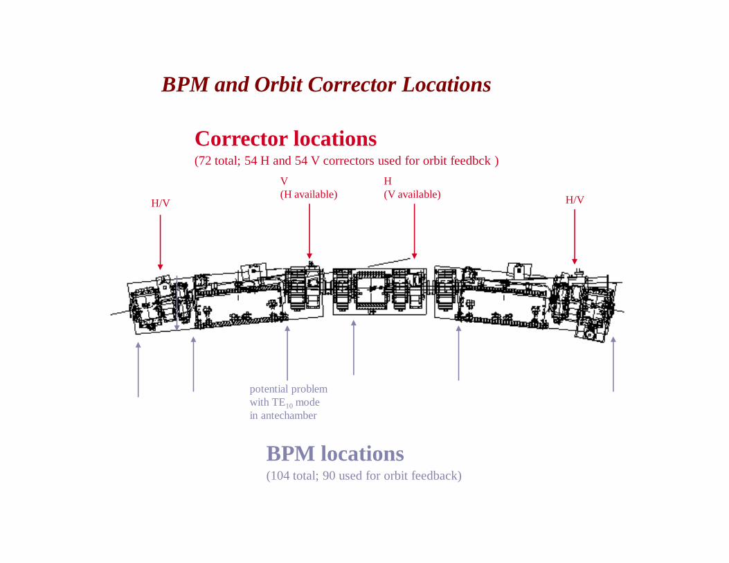
potential problemwith TE10 mode in antechamber

BPM locations(104 total; 90 used for orbit feedback)

Corrector locations(72 total; 54 H and 54 V correctors used for orbit feedbck )

H/V

V(H available) H/V

H(V available)

BPM and Orbit Corrector Locations

BPM Processing and Orbit Feedback Performance Specifications

BPM Processing System Orbit Feedback System

Number BPMs 90 Number electron BPMs 90

Nominal beam current range 1-500 mA Number photon BPMs 11 + future

First turn resolution (.025 nC bunch; .03 mA) 1.8 mm Number correctors 54 H, 54 V

Turn-turn resolution (> 5mA) 12.7 mm Closed-loop bandwidth (-3 dB) 100 Hz

Resolution for fdbk (2 kHz orb update; >5 mA) 1.1 mm (144-turn avg) Component bandwidth

Resolution for 1 s orbit averaging (>5 mA) 0.045 mm (>5 mA) orbit monitor @ 2 kHz update 200 Hz

Resolution parameter (<5 mA; no multiplexing) 0.056 mm-mA/ Hz magnets >1 kHz

Current dependence (for x2 DI ); stability over 24 h <3 mm power supplies 500 Hz

Absolute BPM accuracy wrt quad center* <100 mm vacuum chamber 60 Hz H, 100 Hz V

Dynamic current range (for <10 mm turn-turn res.) 5 mA-500 mA (40 dB) Stability goal (rms at BPMs) <25 mm H,<5 mm V

Position range 1 cm V, 2 cm H

RF button multiplexing 4:1

Button mux switch period (min) ~10 ms / button

Orbit update rate (max) 25 kHz (10 ms/button)

BPM Processing and Orbit Feedback Component Development

RF-IF Converters• 64 BPMs initially; 92 later• Modify existing design for new RF frequency• Considering commercial manufacturer

Digital IF Processors• 8 ea. 8-channel modules (+ spares)• Commercial vendor; 1st units received

Timing/Crate Driver Module• 4 ea. + spares, SLAC design nearly complete

Remote Crate BPM Data Acquisition CPUs• Power PC + 2 PMC slots (Synergy)• RACEway link (PMC) to IF Processors (160 MB/s)• Reflective memory link (PMC) to central crate

>12 Mb/s for each of 4 crates

Orbit Feedback DSP• Dual Power PC + 2 PMC slots (Synergy)• Reflective memory link to 4 remote crates• Fast Ethernet link (PMC) to corrector

supply controllers (100 Mb/s)

Fast Digital Power Supply Controllers• 15 ea (+ spares) crate-based 8-channel

controllers• 4 kHz aggregate update rate with Fast

Ethernet• Digital regulation capability• SLAC design

LO and Timing Generators• Signals derived from 476.3 MHz MO • Commercial low noise design

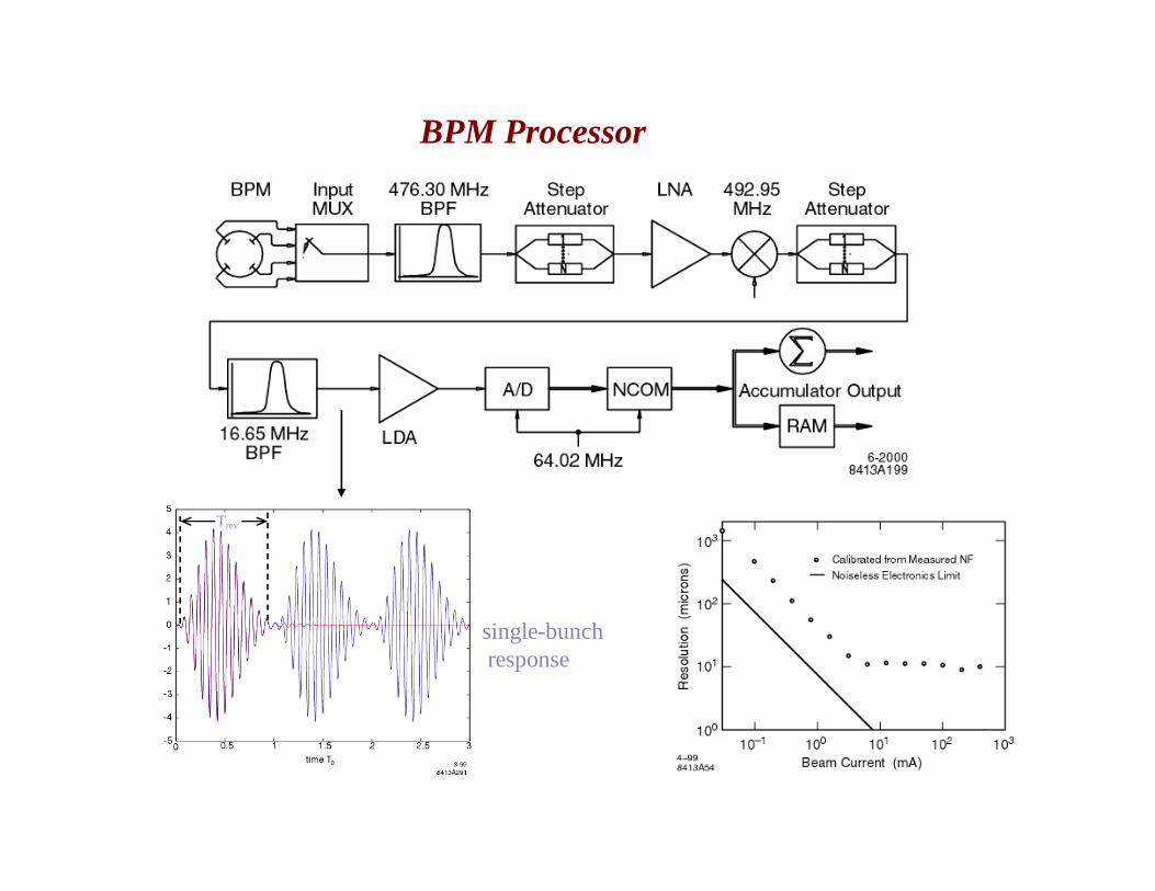
BPM Processor

single-bunchresponse

Trev

BPM Processing - IF Processor

BPM RF-IF Processor Options

4:1 button MUXno BPM MUX

no button MUX4:1 BPM MUX1st turn/singleturn BPM measurement

# BPMs 90

Resolution 1st turn: 1.8 mm (0.03 mA)

turn-turn: 13 mm (> 5 mA)feedback: 1 mm (160 avg)

Current range 5-500 mA (<13 mm turn-turn res)

Current dependency < 3 mm Orbit acquisition rate 2-4 kHz for feedback (~25 kHz max)

RF-IF converter - prototype

8-chan. IF digital processor

BPM Processing

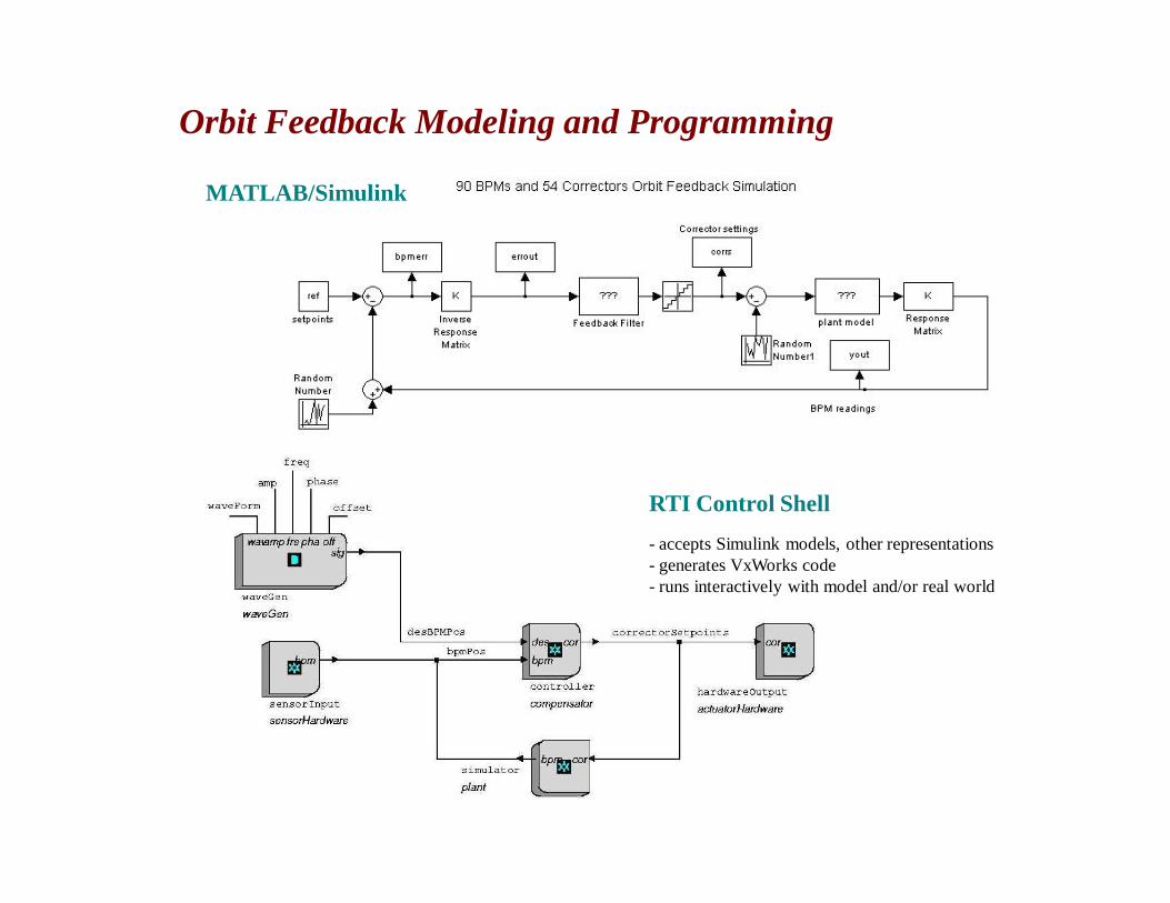
Orbit Feedback Modeling and Programming

RTI Control Shell- accepts Simulink models, other representations - generates VxWorks code- runs interactively with model and/or real world

MATLAB/Simulink

Machine Protection Systems

Vacuum Interlock• PLC 1

• ~160 vacuum chamber water flow switches• ~24 ion gauges• ~310 thermal switches• 12 BL Vacuum OK summaries• Enables RF, ring isolation valves + stoppers• Expand existing system

Magnet Cooling Interlock• PLC 2

• ~20 water flow switches• ~1550 thermal switches/~264 interlock circuits• Enable magnet power supplies• Expand existing system

Chamber Temperature Monitor• PLC 3

• ~375 thermocouples (30-200oC 1oC)• ~16 RTDs (10- 70oC 1oC)• ~960 chan/s measurement rate• Generates alarms, status for Control System• New system, commercially available

Orbit Interlock• Active for beam current >20 mA

less if beam lines open

• 20 BPMs (in beam line areas)future expansion: 2 per new ID; 30 total

•New system designBPM processors: commercial or SLAC designBPLD and Beam Abort: new design, VME components

Orbit Interlock

Coupler Coupler

SpecificationsNumber of BPMs 20Processing frequency 476.3 MHzBeam current range (nom) 5-500 mAResolution (>5 mA) <50 mmAccuracy (wrt quad center) <100 mmDynamic range (intensity) >60 dBChannel isolation >60 dBBeam abort time (via RF system) <1 ms

Interlock Trip Criterion (>20 mA)

ID vertical: ID horizontal:

(uses 2 ea ID straight BPMs per ID, 3 m apart 0.73 mm |y| for angle trip )

Dipole BL vert: |y| < 2.45 mm Dipole BL hor: |x| < 5 mm

(uses upstream ID BPM and downstream dipole BPM per dipole source point)

1mrad49.0y

mm45.2y

1mrad1.1x

mm0.5x

Beam Containment SystemLong Ion Chamber (LION)

Quadrupole Modulation System

DCCT

Parametric Current Transformer (Bergoz)

1 A full scale0.5 mA resolution (1s integration)Dynamic range > 2x107

Absolute accuracy < 0.05%Linearity error < 0.01%DC -100 kHzOutput +/- 10V bipolar113 or 175 mm ID

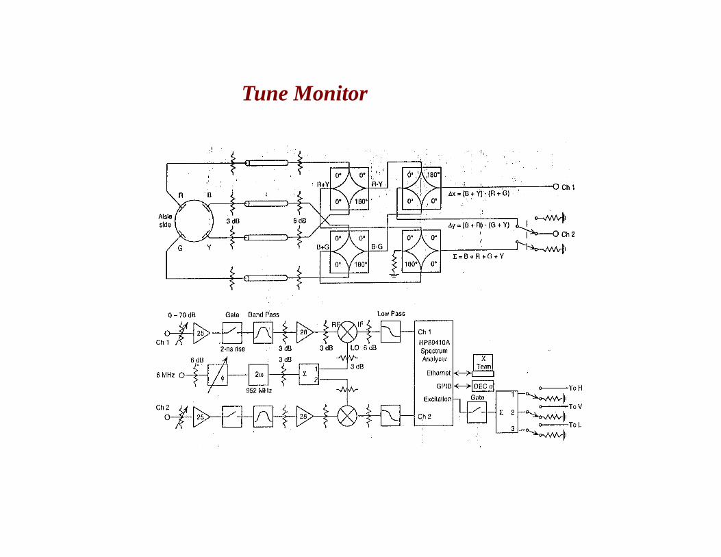
Tune Monitor

Parameter Value

Radius of curvature in dipole r 7.86 mCritical energy in dipole Ec 7.62 keVCritical wavelength in dipole lc 0.163 nmMeasurement wavelength l 210 nmOpening angle (1/g) at lc 0.17 mradOpening angle at l for both polarizations 1.87 mradOpening angle at l for horizontal polarization 1.12 mradDiffraction spot size sd 15 µmElectron beam size sx 183 µmElectron beam size sy 51 µmsy /sd 3.41Vertical image size simage (1:1 image) 53 µmsimage /sy 1.04

Synchrotron Light Monitor

SPEAR 3 Timing and RF Signal Generator System

SPEAR RF: fSPrf = 372 x fSPrev = 476.300 MHz BPM LO: fLO = 385 x fSPrev = 492.935 MHz

Booster RF: fBrf = 280 x fSPrev = 358.505 MHz BPM IF: fIF = 13 x fSPrev = 16.645 MHz

SPEAR revolution freq: fSPrev = 1.2804 MHz IF digitizing clock: fIFclk = 50 x fSPrev = 64.020 MHz

Streak camera clock: fSC = fSPrf/4 = 93 x fSPrev = 119.075 MHz

Wenzel, Inc.

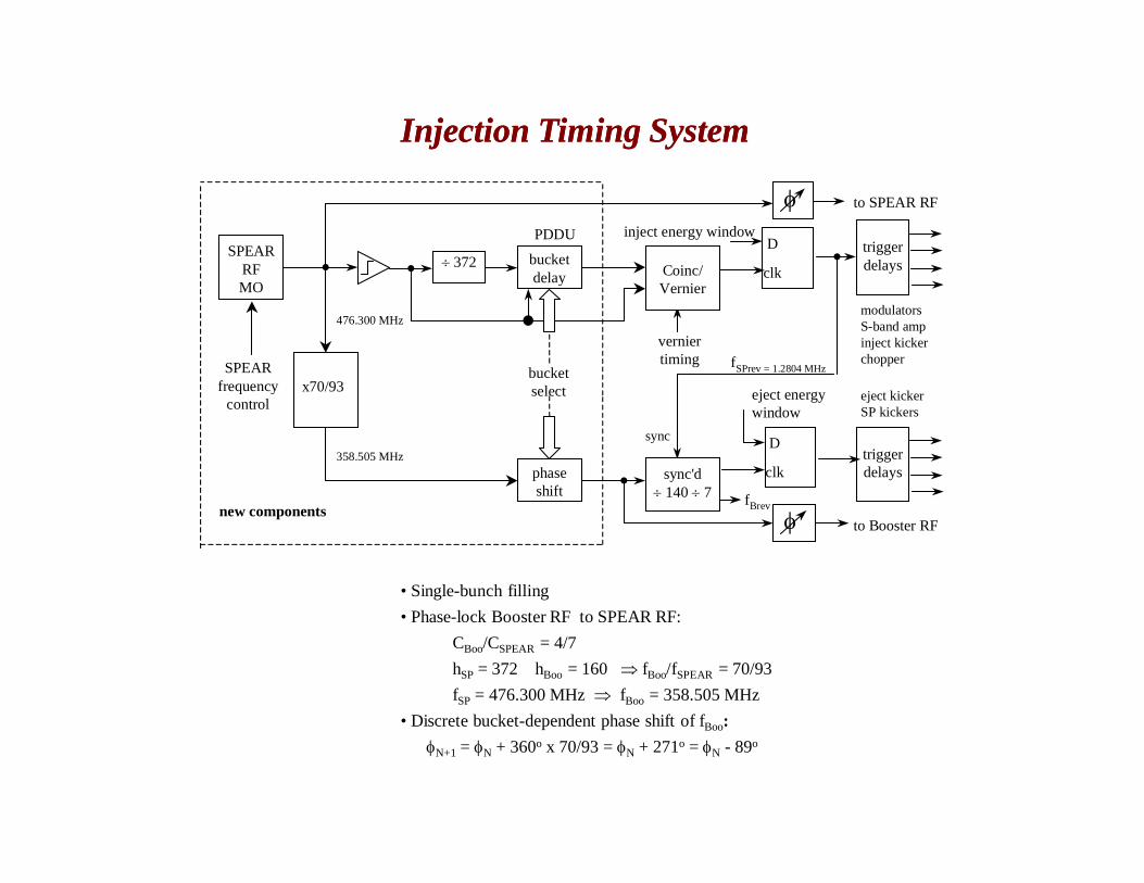
• Single-bunch filling• Phase-lock Booster RF to SPEAR RF:

CBoo/CSPEAR = 4/7 hSP = 372 hBoo = 160 fBoo/fSPEAR = 70/93 fSP = 476.300 MHz fBoo = 358.505 MHz

• Discrete bucket-dependent phase shift of fBoo:N+1 = N + 360o x 70/93 = N + 271o = N - 89o

x70/93bucketselect

SPEARfrequency

control

modulatorsS-band ampinject kickerchopper

SPEARRFMO

372 bucketdelay

D

clk

inject energy windowtriggerdelays

triggerdelays

eject kickerSP kickers

D

clkphaseshift

eject energywindow

sync

to SPEAR RF

fSPrev = 1.2804 MHz

sync'd 140 7 fBrev

476.300 MHz

358.505 MHz

to Booster RFnew components

Coinc/Vernier

verniertiming

PDDU

Injection Timing SystemInjection Timing System

SPEAR 3 Master Oscillator

• 1-500 MHz, DDS-based

• 0.2 Hz step resolution

• Phase-continuous frequency switching

• Stability: 3x10-9/day, 10-6/yr, 10-8/0-50oC

• 0.057o integrated phase noise, 0.5 Hz-15 kHz

• GPIB control

PTS 500

Cable Tray Routes

SPEAR3 CABLE TRAY PLAN

30" Tray from Buildings 117/118 to Ring18" Tray to Shielding Wall Feed Points12" Tray in Matching Cells9" Tray adjacent to girders6" Tray adjacent to Insertion Devices

Power SupplyRoom 118

Main ControlRoom 117

East Pit Building

West Pit Building

Girder Assembly

9" TraySeries ConnectedMagnets

2 ea. 9" TrayI&C, IndividualMagnets, PowerCables

3 ea. 18"Shielding Wall

Feed Trays

30" Cable Trays

3 ea. 18" Trays

*outer shielding notshown

UNIT – IV

Distributed Control Systems

Distributed Control Systems

• Collection of hardware and instrumentation necessary for implementing control systems

• Provide the infrastructure (platform) for implementing advanced control algorithms

History of Control Hardware

• Pneumatic Implementation:

• Transmission: the signals transmitted pneumatically are slow responding and susceptible to interference.

• Calculation: Mechanical computation devices must be relatively simple and tend to wear out quickly.

History (cont.)

• Electron analog implementation:

• Transmission: analog signals are susceptible to noise, and signal quality degrades over long transmission line.

• Calculation: the type of computations possible with electronic analog devices is still limited.

History (cont.)

• Digital Implementation:

• Transmission: Digital signals are far less sensitive to noise.

• Calculation: The computational devices are digital computers.

Advantages of Digital System

Digital computers are more flexible because they are programmable and no limitation to the complexity of the computations it can carry out.

Digital systems are more precise.

Digital system cost less to install and maintain

Digital data in electronic files can be printed out, displayed on color terminals, stored in highly compressed form.

Computer Control Networks

1. PC Control:• Good for small

processes such as laboratory prototype or pilot plants, where the number of control loops is relatively small

PROCESSFinal

controlelement

Dataacquisition

MainComputer

Display


2. Programmable Logic Controllers:• specialized for non-continuous systems such as batch

processes.

• It can be used when interlocks are required; e.g., a flow control loop cannot be actuated unless a pump has been turned on.

• During startup or shutdown of continuous processes.


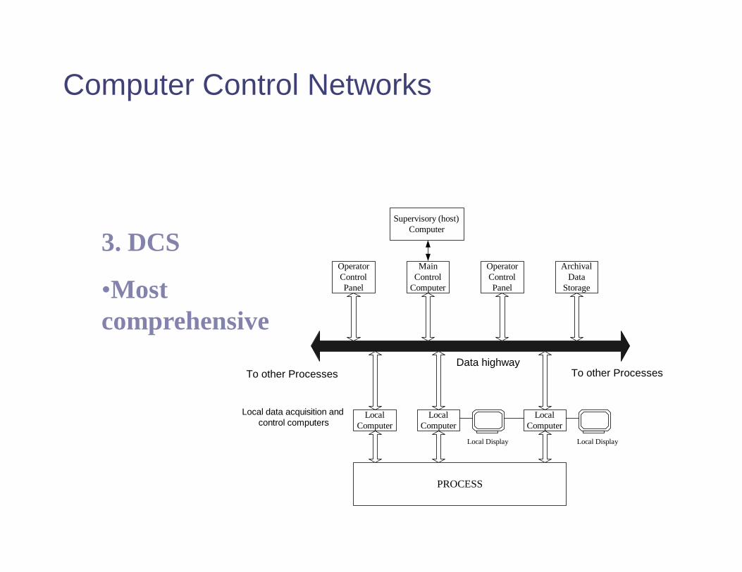
OperatorControlPanel

MainControl

Computer

OperatorControlPanel

ArchivalData

Storage

Supervisory (host)Computer

PROCESS

LocalComputer

LocalComputer

LocalComputer

Local Display Local Display

Data highwayTo other Processes To other Processes

Local data acquisition andcontrol computers

3. DCS

•Most comprehensive

DCS Elements-1

• Local Control Unit: This unit can handle 8 to 16 individual PID loops.

• Data Acquisition Unit: Digital (discrete) and analog I/O can be handle.

• Batch Sequencing Unit: This unit controls a timing counters, arbitrary function generators, and internal logic.

• Local Display: This device provides analog display stations, and video display for readout.

• Bulk Memory Unit: This unit is used to store and recall process data.

DCS Elements-2

• General Purpose Computer : This unit is programmed by a customer or third party to perform optimization, advance control, expert system, etc

• Central Operator Display: This unit typically contain several consoles for operator communication with the system, and multiple video color graphics display units

• Data Highway : A serial digital data transmission link connecting all other components in the system. It allow for redundant data highway to reduce the risk of data loss

• Local area Network (LAN)

Advantages of DCS

Access a large amount of current information from the data highway.

Monitoring trends of past process conditions.

Readily install new on-line measurements together with local computers.

Alternate quickly among standard control strategies and readjust controller parameters in software.

A sight full engineer can use the flexibility of the framework to implement his latest controller design ideas on the host computer.

Modes of Computer control

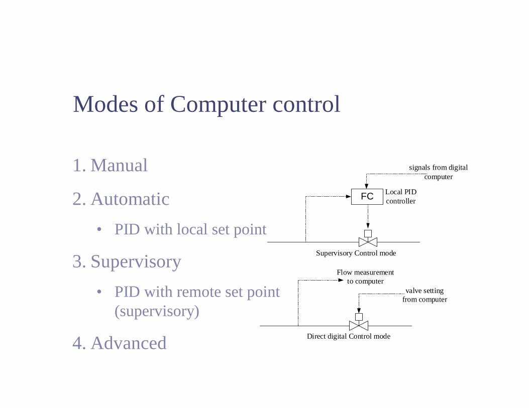
FC

signals from digitalcomputer

Local PIDcontroller

Supervisory Control mode

Direct digital Control mode

valve settingfrom computer

Flow measurementto computer

1. Manual

2. Automatic• PID with local set point

3. Supervisory• PID with remote set point

(supervisory)

4. Advanced

Additional Advantage

Digital DCS systems are more flexible. Control algorithms can be changed and control configuration can be modified without having rewiring the system.

Categories of process information

ExampleType

Relay, Switch Solenoid valveMotor drive

1. Digital

Alphanumerical displays2. Generalized digital

Turbine flow meterStepping motor

3. Pulse

Thermocouple or strain gauge (mill volt)Process instrumentation (4-20 am)Other sensors (0-5 Volt)

4. Analog

Interface between digital computer and analog instruments

• (A/D) Transducers convert analog signals to digital signals. (Sensor Computer)

• (D/A) Transducers convert digital signals to analog signals. (Computer Valve)

Data resolution due to digitization

• Accuracy depends on resolution.• Resolution depends on number of bits:

Resolution = signal range × 1/(2m -1)

m = number of bits used by the digitizer (A/D) to represent the analog data

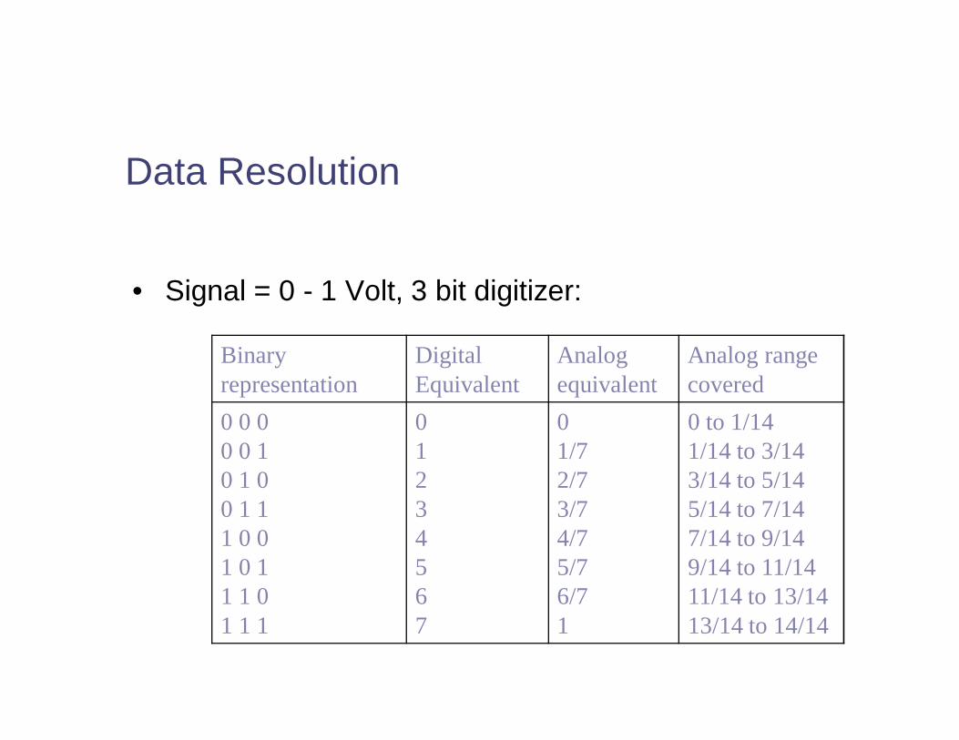
Data Resolution

• Signal = 0 - 1 Volt, 3 bit digitizer:

Analog range covered

Analog equivalent

Digital Equivalent

Binary representation

0 to 1/141/14 to 3/143/14 to 5/145/14 to 7/147/14 to 9/149/14 to 11/1411/14 to 13/1413/14 to 14/14

01/72/73/74/75/76/71

01234567

0 0 00 0 10 1 0 0 1 1 1 0 01 0 11 1 01 1 1

Data Resolution

0 1/7 2/7 3/7 4/7 5/7 6/7 10

1

2

3

4

5

6

7

Analog data

Dig

ital d

ata

Utilization of DCS

• DCS vendor job:• installation

• Control Engineer Job:• Configuration

• Built-in PID control:• How to Tune the PID control?

Utilization of DCS

• Implementation of advanced control:

• Developed software for control algorithms, DMC, Aspen, etc.

• Control-oriented programming language supplied by the DCS vendors.

• Self-developed programs using high-level programming languages (Fortran, C++)

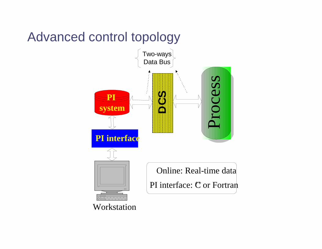
Advanced control topology

DC

S

WorkstationPr

oces

s

Two-waysData Bus

Online: Real-time data

PI interface

PI interface: C++ or Fortran

PIsystem

DCS Vendors

• Honeywell• Fisher-Rosemont• Baily• Foxboro• Yokogawa

• Siemen

Unit V INTERFACES IN DCS

Sections:1. Process Industries vs. Discrete Manufacturing

Industries2. Continuous vs. Discrete Control3. Computer Process Control

Industrial Control - Defined

The automatic regulation of unit operations and their associated equipment as well as the integration and coordination of the unit operations into the larger production system

• Unit operation• Usually refers to a manufacturing operation• Can also apply to material handling or other equipment

Process Industries vs. Discrete Manufacturing Industries

• Process industries• Production operations are performed on amounts of

materials• Materials: liquids, gases, powders, etc.

• Discrete manufacturing industries• Production operations are performed on quantities of

materials• Parts, product units

Definitions: Variable and Parameters

• Variables - outputs of the process• Parameters - inputs to the process• Continuous variables and parameters - they are

uninterrupted as time proceeds• Also considered to be analog - can take on any value

within a certain range• They are not restricted to a discrete set of values

• Discrete variables and parameters - can take on only certain values within a given range

Discrete Variables and Parameters

Categories:• Binary - they can take on either of two possible

values, ON or OFF, 1 or 0, etc.• Discrete other than binary - they can take on

more than two possible values but less than an infinite number of possible values

• Pulse data - a train of pulses that can be counted

Continuous and Discrete Variables and Parameters

Types of Control• Just as there are two basic types of variables and

parameters in processes, there are also two corresponding types of control:• Continuous control - variables and parameters are

continuous and analog• Discrete control - variables and parameters are

discrete, mostly binary discrete

Continuous Control

• Usual objective is to maintain the value of an output variable at a desired level• Parameters and variables are usually continuous• Similar to operation of a feedback control system• Most continuous industrial processes have

multiple feedback loops• Examples of continuous processes:

• Control of the output of a chemical reaction that depends on temperature, pressure, etc.

• Control of the position of a cutting tool relative to workpart in a CNC machine tool

Types of Continuous Process Control

• Regulatory control• Feedforward control• Steady-State optimization• Adaptive control• On-line search strategies• Other specialized techniques

• Expert systems• Neural networks

Regulatory Control

• Objective - maintain process performance at a certain level or within a given tolerance band of that level• Appropriate when performance relates to a quality

measure• Performance measure is sometimes

computed based on several output variables• Performance measure is called the Index of

performance (IP)• Problem with regulatory control is that an

error must exist in order to initiate control action

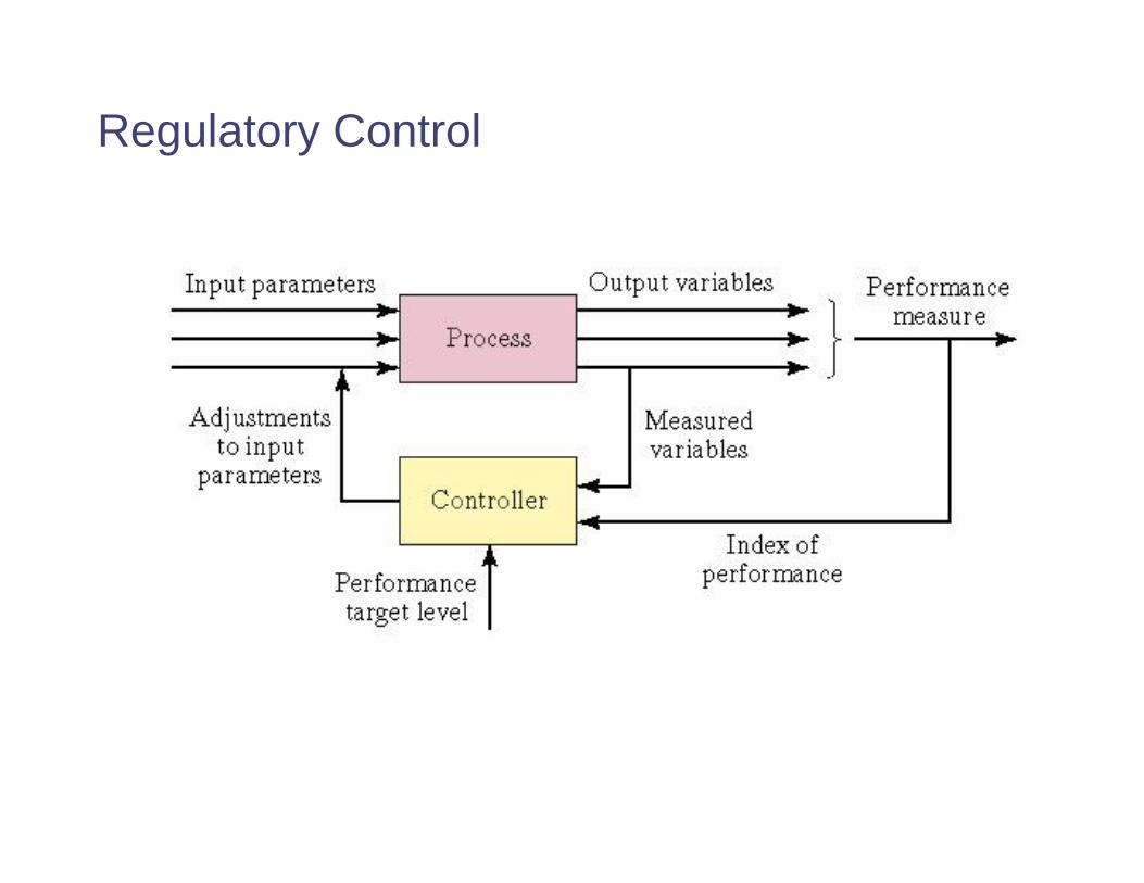
Regulatory Control

Feedforward Control

• Objective - anticipate the effect of disturbances that will upset the process by sensing and compensating for them before they affect the process

• Mathematical model captures the effect of the disturbance on the process

• Complete compensation for the disturbance is difficult due to variations, imperfections in the mathematical model and imperfections in the control actions• Usually combined with regulatory control

• Regulatory control and feedforward control

Feedforward Control Combined with Feedback Control

Steady-State Optimization

Class of optimization techniques in which the process exhibits the following characteristics:1. Well-defined index of performance (IP)2. Known relationship between process variables

and IP3. System parameter values that optimize IP can be

determined mathematically• Open-loop system• Optimization techniques include differential

calculus, mathematical programming, etc.

Steady State (Open-Loop) Optimal Control

Adaptive Control

• Because steady-state optimization is open-loop, it cannot compensate for disturbances

• Adaptive control is a self-correcting form of optimal control that includes feedback control• Measures the relevant process variables during

operation (feedback control)• Uses a control algorithm that attempts to optimize some

index of performance (optimal control)

Adaptive Control Operates in a Time-Varying Environment

• The environment changes over time and the changes have a potential effect on system performance• Example: Supersonic aircraft operates differently in

subsonic flight than in supersonic flight• If the control algorithm is fixed, the system may

perform quite differently in one environment than in another

• An adaptive control system is designed to compensate for its changing environment by altering some aspect of its control algorithm to achieve optimal performance

Three Functions in Adaptive Control

1. Identification function – current value of IP is determined based on measurements of process variables

2. Decision function – decide what changes should be made to improve system performance• Change one or more input parameters • Alter some internal function of the controller

3. Modification function – implement the decision function• Concerned with physical changes (hardware

rather than software)

Adaptive Control System

On-Line Search Strategies

• Special class of adaptive control in which the decision function cannot be sufficiently defined• Relationship between input parameters and IP is

not known, or not known well enough to implement the previous form of adaptive control

• Instead, experiments are performed on the process• Small systematic changes are made in input

parameters to observe effects• Based on observed effects, larger changes

are made to drive the system toward optimal performance

Discrete Control Systems

• Process parameters and variables are discrete

• Process parameters and variables are changed at discrete moments in time

• The changes are defined in advance by the program of instructions

• The changes are executed for either of two reasons:1. The state of the system has changed (event-

driven changes)2. A certain amount of time has elapsed (time

driven changes)

Event-Driven Changes

• Executed by the controller in response to some event that has altered the state of the system

• Examples:• A robot loads a workpart into a fixture, and the part

is sensed by a limit switch in the fixture• The diminishing level of plastic in the hopper of an

injection molding machine triggers a low-level switch, which opens a valve to start the flow of more plastic into the hopper

• Counting parts moving along a conveyor past an optical sensor

Time-Driven Events

• Executed by the controller either at a specific point in time or after a certain time lapse

• Examples:• The factory “shop clock” sounds a bell at specific

times to indicate start of shift, break start and stop times, and end of shift

• Heat treating operations must be carried out for a certain length of time

• In a washing machine, the agitation cycle is set to operate for a certain length of time

• By contrast, filling the tub is event-driven

Two Types of Discrete Control

1. Combinational logic control – controls the execution of event-driven changes• Also known as logic control• Output at any moment depends on the values of

the inputs• Parameters and variables = 0 or 1 (OFF or ON)

2. Sequential control – controls the execution of time-driven changes• Uses internal timing devices to determine when

to initiate changes in output variables

Computer Process Control

• Origins in the 1950s in the process industries• Mainframe computers – slow, expensive, unreliable• Set point control• Direct digital control (DDC) system installed 1962

• Minicomputer introduced in late 1960s, microcomputer introduced in early 1970s

• Programmable logic controllers introduced early 1970s for discrete process control

• Distributed control starting around 1975• PCs for process control early 1990s

Two Basic Requirements for Real-Time Process Control

1. Process-initiated interrupts • Controller must respond to incoming signals from

the process (event-driven changes)• Depending on relative priority, controller may have

to interrupt current program to respond2. Timer-initiated actions

• Controller must be able to execute certain actions at specified points in time (time-driven changes)

• Examples: (1) scanning sensor values, (2) turning switches on and off, (3) re-computing optimal parameter values

Other Computer Control Requirements

3. Computer commands to process • To drive process actuators

4. System- and program-initiated events• System initiated events - communications between

computer and peripherals• Program initiated events - non-process-related

actions, such as printing reports5. Operator-initiated events – to accept input from

personnel• Example: emergency stop

Capabilities of Computer Control

• Polling (data sampling)• Interlocks• Interrupt system• Exception handling

Polling (Data Sampling)

Periodic sampling of data to indicate status of process

• Issues:1. Polling frequency – reciprocal of time interval

between data samples2. Polling order – sequence in which data collection

points are sampled3. Polling format – alternative sampling procedures:

• All sensors polled every cycle• Update only data that has changed this cycle• High-level and low-level scanning

Interlocks

Safeguard mechanisms for coordinating the activities of two or more devices and preventing one device from interfering with the other(s)

1. Input interlocks – signal from an external device sent to the controller; possible functions:• Proceed to execute work cycle program• Interrupt execution of work cycle program

2. Output interlocks – signal sent from controller to external device

Interrupt System

Computer control feature that permits the execution of the current program to be suspended in order to execute another program in response to an incoming signal indicating a higher priority event

• Internal interrupt – generated by the computer itself• Examples: timer-initiated events, polling, system-

and program initiated interrupts• External interrupts – generated external to

the computer• Examples: process-initiated interrupts, operator

inputs

Interrupt Systems:(a) Single-Level and (b) Multilevel

(a)

(b)

Exception Handling

An exception is an event that is outside the normal or desired operation of the process control system

• Examples of exceptions:• Product quality problem• Process variable outside normal operating range• Shortage of raw materials• Hazardous conditions, e.g., fire• Controller malfunction

• Exception handling is a form of error detection and recovery

Forms of Computer Process Control

1. Computer process monitoring2. Direct digital control (DDC)3. Numerical control and robotics4. Programmable logic control 5. Supervisory control6. Distributed control systems and personal

computers

Computer Process Monitoring

Computer observes process and associated equipment, collects and records data from the operation

• The computer does not directly control the process• Types of data collected:

• Process data – input parameters and output variables• Equipment data – machine utilization, tool change

scheduling, diagnosis of malfunctions• Product data – to satisfy government requirements,

e.g., pharmaceutical and medical

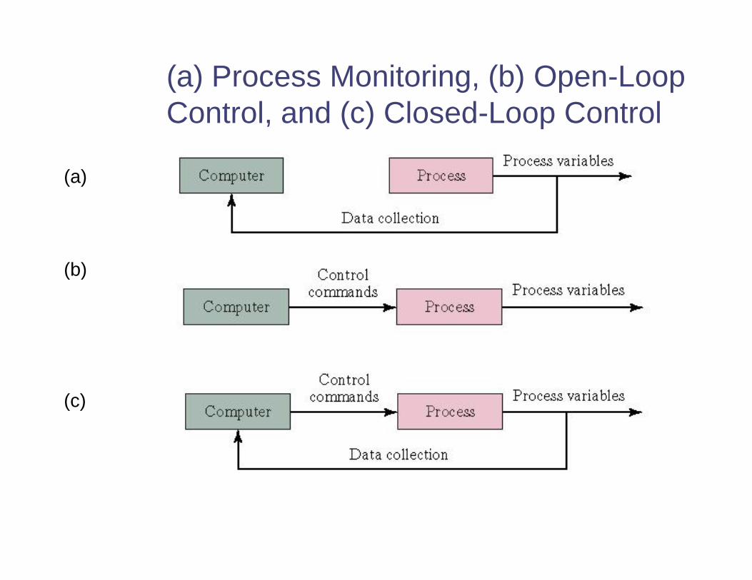
(a) Process Monitoring, (b) Open-Loop Control, and (c) Closed-Loop Control

(a)

(b)

(c)

Direct Digital Control (DDC)

Form of computer process control in which certain components in a conventional analog control system are replaced by the digital computer

• Circa: 1960s using mainframes• Applications: process industries• Accomplished on a time-shared, sampled-data basis

rather than continuously by dedicated components• Components remaining in DDC: sensors and actuators• Components replaced in DDC: analog controllers, recording

and display instruments, set point dials

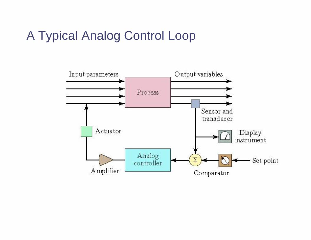
A Typical Analog Control Loop

Components of a Direct Digital Control System

DDC (continued)

• Originally seen as a more efficient means of performing the same functions as analog control

• Additional opportunities became apparent in DDC:• More control options than traditional analog control

(PID control), e.g., combining discrete and continuous control

• Integration and optimization of multiple loops• Editing of control programs

Numerical Control and Robotics

• Computer numerical control (CNC) –computer directs a machine tool through a sequence of processing steps defined by a program of instructions• Distinctive feature of NC – control of the position

of a tool relative to the object being processed• Computations required to determine tool trajectory

• Industrial robotics – manipulator joints are controlled to move and orient end-of-arm through a sequence of positions in the work cycle

Programmable Logic Controller (PLC)

Microprocessor-based controller that executes a program of instructions to implement logic, sequencing, counting, and arithmetic functions to control industrial machines and processes

• Introduced around 1970 to replace electromechanical relay controllers in discrete product manufacturing

• Today’s PLCs perform both discrete and continuous control in both process industries and discrete product industries

Supervisory Control

In the process industries, supervisory control denotes a control system that manages the activities of a number of integrated unit operations to achieve certain economic objectives

In discrete manufacturing, supervisory control is the control system that directs and coordinates the activities of several interacting pieces of equipment in a manufacturing system• Functions: efficient scheduling of production, tracking tool

lives, optimize operating parameters

• Most closely associated with the process industries

Supervisory Control Superimposed on Process Level Control System

Distributed Control Systems (DCS)

Multiple microcomputers connected together to share and distribute the process control workload

• Features:• Multiple process control stations to control individual

loops and devices• Central control room where supervisory control is

accomplished• Local operator stations for redundancy• Communications network (data highway)

Distributed Control System

DCS Advantages

• Can be installed in a very basic configuration, then expanded and enhanced as needed in the future

• Multiple computers facilitate parallel multitasking• Redundancy due to multiple computers• Control cabling is reduced compared to central

controller configuration• Networking provides process information

throughout the enterprise for more efficient plant and process management

PCs in Process Control

Two categories of personal computer applications in process control:

1. Operator interface – PC is interfaced to one or more PLCs or other devices that directly control the process• PC performs certain monitoring and supervisory

functions, but does not directly control process 2. Direct control – PC is interfaced directly to

the process and controls its operations in real time• Traditional thinking is that this is risky

Enablers of PCs for Direct Control

• Widespread familiarity of workers with PCs• Availability of high performance PCs

• Cycle speeds of PCs now exceed those of PLCs• Open architecture philosophy in control

system design• Hardware and software vendors comply with

standards that allow their products to be interoperable

• PC operating systems that facilitate real-time control and networking

• PC industrial grade enclosures

Enterprise-Wide Integration of Factory Data

• Managers have direct access to factory operations• Planners have most current data on production times

and rates for scheduling purposes• Sales personnel can provide realistic delivery dates

to customers, based on current shop loading• Order trackers can provide current status information

to inquiring customers• QC can access quality issues from previous orders• Accounting has most recent production cost data• Production personnel can access product design

data to clarify ambiguities

Enterprise-Wide PC-based Distributed Control System

logic and distributed control system - biher · computer control system expand present control...

Documents