logarithmic wind proﬁle: a stability wind shear term

arX

iv:1

405.

5158

v1 [

phys

ics.

ao-p

h] 2

0 M

ay 2

014

LAB Template

Template 2014; 00:1–14DOI: xx.xxxx/xx

RESEARCH ARTICLE

Logarithmic Wind Profile: A Stability Wind Shear TermYoshiaki Sakagami1,2, Pedro A. A. Santos2, Reinaldo Haas3, Julio C. Passos2, Frederico F. Taves4

1 Dept. of Health and Service, Federal Institute of Santa Catarina, Florianopolis, Brazil2 Dept. of Mechanical Engineering, Federal University of Santa Catarina, Florianopolis, Brazil3 Dept. of Physics, Federal University of Santa Catarina, Florianopolis, Brazil4 Tractebel Energia S.A. (GDF Suez), Florianopolis, Brazil

ABSTRACT

A stability wind shear term of logarithmic wind profile basedon the terms of turbulent kinetic energy equation is proposed.The fraction influenced by thermal stratification is considered in the shear production term. This thermally affected shearis compared with buoyant term resulting in a stability wind shear term. It is also considered Reynolds stress as a sum oftwo components associated with wind shear from mechanical and thermal stratification process. The stability wind shearisresponsible to Reynolds stress of thermal stratification term, and also to Reynolds stress of mechanical term at no neutralcondition. The wind profile and its derivative are validatedwith data from Pedra do Sal experiment in a flat terrain and300m from shoreline located in northeast coast of Brazil. Itis close to the Equator line, so the meteorological condition arestrongly influenced by trade winds and sea breeze. The site has one 100m tower with five instrumented levels, one 3D sonicanemometer, and a medium-range wind lidar profiler up 500 m. The dataset are processed and filter from September toNovember of 2013 which results in about 550 hours of data available. The results show the derivative of wind profile withR2 of 0.87 and RMSE of 0.08m s−1. The calculated wind profile performances well up to 400 m at unstable conditionand up to 280 m at stable condition withR2 better than 0.89. The proposed equation is valid for this specific site and islimited to a stead state condition with constant turbulent fluxes in the surface layer. Copyrightc© 2014 Lepten.

KEYWORDS

Atmospheric Stability, Lidar Measurements, Logarithmic Wind Profile, Eddy Covariance

Correspondence

Yoshiaki Sakagami,Dep. of Health and Service, Federal Institute of Santa Catarina, Florianopolis, Brazil.

E-mail: [email protected]

Received . . .

1. INTRODUCTION

The study of wind speed profile in the atmospheric boundary layer has progressed recently by new technologies such assodar and lidar profilers, and better eddy covariance systems. The theory of wind profile that is based on semi-empirical thelogarithmic law that is well correlated at neutral conditions. However, the atmosphere is rarely neutral, and turbulence hasa strong influence on the wind speed profile. The turbulence isrelated to atmospheric stability concept when unstable flowbecome or remain turbulent and stable flow become or remain laminar [1]. The cornerstone of this problem is that the windprofile need to be correct not just by the slope of logarithmicprofile but its shape [2]. It also depends on a stability parameterthat is not well understood because of stochastic nature of turbulent process. The most common parameter used to quantifythe atmospheric stability is the Obukhov length (L) based onthe Monin-Obukhov similarity theory [3]. Many experimentsconducted in the last 50 years have showed a good agreements to the similarity theory with an accuracy of about 10-20%[4], [5], [6], [7]. They suggests many different parameters to the universalsimilarity function and the accepted functionpresently is the re-formulated function from Businger et al. [8] proposed by Hogstrom [6] [7]. However, the experimentsare located at specific sites and limited to particular meteorological conditions. Recent studies about atmospheric stabilityrelated to wind turbines performance diverges for each specific site condition [9], [10],[11], [12],[13]), [14]. This is one ofthe gaps for wind energy applications and a better understanding of the wind profile and other properties such as turbulenceand stability is necessary [15]. Other important studies are related to the improvements of micro siting models for wind

Copyright c© 2014 Lepten. 1

http://arxiv.org/abs/1405.5158v1

Logarithmic Wind Profile: A Stability Wind Shear Term Sakagami Y. et al.

energy application [16] and the numerical weather predictions models [17] as the boundary layer in those models are stillpoor represented [18]. The limits of the actual theory and particular results suggest that a local experiment is necessarywhen wind profile need to be accurate predict at a specific site. Thus, an experiment is set in Pedra do Sal Wind Farmlocated in north-east coast of Brazil when the meteorological condition are strongly influenced by trade winds and seabreeze. A instrumented tower of 100m with five levels of wind measurements, one sonic 3D anemometer and one lidarwind profiler is used. Based on the analysis of this data and the turbulent kinetic energy equation, a stability wind shearterm of the logarithmic wind profile is proposed. The equation is compared with data of this experiment and is showed inthe results section. The limits of this equation and conclusions are presented in the last section.

2. THEORY

2.1. Shear Components

The hypothesis of Eddy viscosity, suggested by J. Boussinesq in 1877 [19], assumes that Reynolds stress (τ ) can beanalogous with Newton’s law of molecular viscosity. Considering the coordinate system aligned with the mean flow andhorizontal mean gradients neglected in comparison to thosein vertical at the surface layer,τ can be expressed as:

τ = −ρu′w′ = ρKm∂U

∂z(1)

where theKm is known as eddy exchange of momentum or simply eddy viscosity, ρ is the air density,U is the horizontalmean flow andu andw are the horizontal and vertical wind speed component respectively and the apostrophes are thedeviations from their means. Eq.1 represents the total Reynolds stress, but it maybe be view asa sum of two componentsassuming that at a given height forced and free convection are mutually independent [20]. One part has a eddy viscositycoefficient associated with forced convection and another due free convection. Similar to this assumption, it is assumethatReynolds stress can be divide in two components as well, but each component is related to wind shear instead of eddyviscosity:

τ = τm + τs (2)

whereτm term is associated with wind shear produced/loss by mechanical process (∂Um/∂z) andτs term is associatedwith wind shear produced/consumed by thermal stratification process (∂Us/∂z). Then, combining Eq.1 and Eq.2:

ρKm∂U

∂z= ρKm

∂Um

∂z+ ρKm

∂Us

∂z(3)

It is considered the flow incompressible and coefficients of eddy viscosity at neutral condition in the surface layer. Then,the sum of Reynolds stress can be express as a simply sum of wind shear:

∂U

∂z=∂Um

∂z+∂Us

∂z(4)

The mechanical and thermal stratified process associated with wind shear are described in details in next section.

2.2. Thermal Stratified Shear

The turbulence kinetic energy (TKE) is one of the most important variable in the boundary layer and its budget equationdescribes the physical process that produce/consume the turbulence [1]. The simplify form of TKE budget equation, basedon horizontal homogeneity, neglect subsidence and coordinate system aligned with the mean flow can be expressed by:

∂e

∂t=

g

θv(w′θ′v)− u′w′

∂U

∂z− ∂(w′e)

∂z− 1

ρ

∂(w′p′)

∂z− ε (5)

where the terms represent: the storage, buoyant, shear, transport, pressure perturbation and dissipation, respectively. Theturbulence kinetic energy ise, θv is the potential virtual temperature,g is the gravitational acceleration,u andw are thehorizontal and vertical wind speed component respectively, U is the horizontal mean flow,p is the atmospheric pressureandρ is the air density. The variables with apostrophes are the deviations from their means and the bar symbol is thevariable average. The difficult to study the turbulence is that it a dissipative process and its equation is not conservative[1]. Then, the atmospheric stability is usually analysed by comparing terms of this equation as dimensionless ratio such asflux Richardson number (Rf ), even though the other terms in the TKE budget are also important:

2 Template 2014; 00:1–14 c© 2014 Lepten.DOI: 10.1002/xx

Prepared using template.cls

Sakagami Y. et al. Logarithmic Wind Profile: A Stability Wind Shear Term

Rf =

g

θv(w′θ′v)

−u′w′ ∂U∂z

(6)

This ratio is modified by a new Richardson number, named asRis. It is assumed thatRis represents only the windshear associated with thermal stratification (∂Us/∂z).

Ris =

g

θv(w′θ′v)

−u′w′ ∂Us

∂z

(7)

It means thatRis is proportion of the rate at which the energy is produced/consumed by the buoyant term and the rate atwhich the energy is produced/loss by the fraction of wind shear related to thermal stratification. This proportion is assumedto be constant in steady-state condition, soRis is considered a constant coefficient in the equation and can be determinedfrom experimental data (Fig.6).

− u′w′∂Us

∂zRis =

g

θv(w′θ′v) (8)

The turbulent fluxes of momentum and heat can also be rewritten in terms of sensible heat flux (Hs) and friction velocity(u∗) [19]. Then, the wind shear related to thermal stratification canbe express as:

∂Us

∂z=

−gHs

ρcpθvu2∗Ris

(9)

wherecp is the specific heat of dry air at constant pressure. This termis simply named as stability wind shear. It is directresponsible to Reynolds stressτs and also to influence the mechanical wind shear at no neutral condition, which is showin the next section.

2.3. Mechanical Shear

The Reynolds stressτm is associated with wind shear produced by mechanical process (∂Um/∂z). At neutral condition,the mechanical wind shear isu∗/(κz), whereκ is the von Karman constant and z is the height. However, themechanicalwind shear is influenced by thermal stratification process atno neutral conditions. Then, it is assume that mechanicalReynolds stress can be divided in two terms:

τm = τn + τnn (10)

whereτn is associated with wind shear at neutral condition (∂Un/∂z) andτnn is associated with the fraction of windshear influenced by thermal stratification process at no neutral condition (∂Unn/∂z).

ρKm∂Um

∂z= ρKn

∂Un

∂z+ ρKnn

∂Unn

∂z(11)

The eddy viscosity can not be considered at neutral condition to all coefficients in this case. Each term has itsown coefficient of eddy viscosity related to its wind shear. Then,Km = l2m|∂Um/∂z|, Kn = l2m|∂Un/∂z| andKnn =l2m|∂Unn/∂z|, andlm is the mean mix length.

ρl2m

(

∂Um

∂z

)2

= ρl2m

(

∂Un

∂z

)2

+ ρl2m

(

∂Unn

∂z

)2

(12)

It is considered the flow incompressible and the mixing length constant at each height in the surface layer (lm = κz).

(

∂Um

∂z

)2

=

(

∂Un

∂z

)2

+

(

∂Unn

∂z

)2

(13)

Simplifying the Eq.13, the mechanical wind shear influenced by thermal stratification process at no neutral conditioncan be express as:

∂Um

∂z=

√

√

√

√

(

∂Un

∂z

)2

+

(

∂Unn

∂z

)2

(14)

where the wind shear at neutral condition is:

Template 2014; 00:1–14 c© 2014 Lepten. 3DOI: 10.1002/xxPrepared using template.cls


∂Un

∂z=u∗

κz(15)

and fraction of wind shear affected by thermal process at no neutral condition is assume to be equals to stability windshear (Eq.9).

∂Unn

∂z=∂Us

∂z(16)

2.4. Total Shear

The total wind shear can be express by combining Eq.4, Eq.9, Eq.14.

∂U

∂z=

√

√

√

√

(

u∗

κz

)

2

+

(

−gHs

ρcpθvu2∗Ris

)

2

− gHs

ρcpθvu2∗Ris

(17)

2.5. Wind Profile

The terms of the Eq.17 can be renamed to simplify the equation.

∂U

∂z= ψ + ψs (18)

where

ψ =

√

√

√

√

(

u∗

κz

)2

+ ψ2s (19)

and

ψs =−gHs

ρcpθvu2∗Ris

(20)

The turbulent fluxes of heat and momentum can be considered constants with the height in the surface layer [3], and thewind profile can be found by integrating Eq.18.

∫

∂U =

∫

(ψ + ψs)∂z (21)

Solving this integral, the logarithmic wind speed profile with wind shear stability term can be written as:

U(z) =u∗

κln

(

z

zo

)

+ (ψz − ψozo)− u∗

κln

(

ψz + u∗

κ

ψozo +u∗

κ

)

+ ψsz (22)

wherezo is the coefficient roughness andψo is the mechanical shear atzo.

2.6. Reference Shear

The dimensionless shear (φm) introduced by Obukhov [3] is widely used as a parameter to study the influence of theatmospheric stability on the wind profile.

φm =κz

u∗

∂U(z)

∂z(23)

The ratio of von Karman constant and friction velocity (κ/u∗) in the equation can be viewed as a slope correction duemechanical stability. Therefore, the dimensionless shearis not in fact the slope of the wind profile observed, but a slopecorrected by friction velocity. In order to analyse the slope of wind profile without mechanical corrections, the ratioκ/u∗

is omitted from dimensionless shear equation, and a simplified reference shear (φr) is adopted.

φr =z∂U(z)

∂z(24)

The reference shear can be calculated using the measurements of the wind speed at several heights and approximatingthe profile by a second-order polynomial [6].




u(z) = uo + Aln(z) +B(ln(z))2 (25)

where the coefficientsuo, A and B can be found by adjusting the best polynomial fitting.The polynomial equation above is derived, so the reference shear observed can be expressed as:

φr = A+ 2Bln(zm) (26)

wherezm is the geometric mean height for logarithmic approximation[19].

zm =√zhighzlow (27)

where, high and low labels are the top and button levels of themeasurements. The theoretical reference shear (φs) isestimated by Eq.18 multiplied byzm.

φs = zm(ψ + ψs) (28)

The observed and calculated reference shear are compared bylinear fitting andRis can be estimated at the bestcoefficient of determination.

3. EXPERIMENT

3.1. Site description

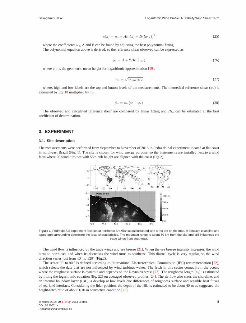
The measurements were performed from September to Novemberof 2013 in Pedra do Sal experiment located at flat coastin north-east Brazil (Fig.1). The site is chosen for wind energy purpose, so the instruments are installed next to a windfarm where 20 wind turbines with 55m hub height are aligned with the coast (Fig.2).

Figure 1. Pedra do Sal experiment location at northeast Brazilian coast indicated with a red dot on the map. A concave coastline andtopograph surrounding determine the local characteristics. The mountain range is about 80 km from the site and still influences the

trade winds from southeast.

The wind flow is influenced by the trade winds and sea breeze [21]. When the sea breeze intensity increases, the windturns to north-east and when its decreases the wind turns to southeast. This diurnal cycle is very regular, so the winddirection varies just from40◦ to 120◦ (Fig.2).

The sector0 ◦ to 90 ◦ is defined according to International Electrotechnical Commission (IEC) recommendation [22],which selects the data that are not influenced by wind turbines wakes. The fetch in this sector comes from the ocean,where the roughness surface is dynamic and depends on the Reynolds stress [23]. The roughness length (zo) is estimatedby fitting the logarithmic equation (Eq.22) on averaged observed profiles [24]. The air flow also cross the shoreline, andan internal boundary layer (IBL) is develop at low levels duedifferences of roughness surface and sensible heat fluxesof sea-land interface. Considering the lidar position, thedepth of the IBL is estimated to be about 40 m as suggested theheight-fetch ratio of about 1/10 in convective condition [25].



5%

10%

15%

20%

WEST EAST

SOUTH

NORTH

0

4

8

12

16

20

[ m s−1 ]

a. Sector0◦ to 90◦ b. Wind Rose

Figure 2. (a.) Satellite image from Pedra do Sal Wind Farm. The picture shows wind turbines aligned with the coast, the position ofthe lidar marked in red circle and the meteorological tower in blue circle. The black circle indicates the distance from lidar to tower,and the red lines represents the limits of the sector free of wake (0 ◦ to 90 ◦). (b.) The wind rose at Pedra do Sal considering allevents from September to November of 2013 (no filtered). Unique condition where winds blew only from 35.3 ◦ to 144.1 ◦ in three

consecutive months.

3.2. Measurements

Pedra do Sal experiment has one meteorological tower of 100mheight with five levels measurements and one mediumrange lidar wind profiler, see details on TableI. The lidar is positioned about 100m in front of the turbines (upwind), and565m away from the tower (Fig2). The mounting of instruments on the tower are in accordanceto IEC norm [22], and thecup anemometers and the ultrasonic are calibrated in wind tunnel.

Table I. Meteorological instruments installed at Pedra do Sal experiment. All sensors are mounted on the tower with 100 m height,except the lidar which is 565 m away from the tower.

Instrument Measurement Height Scan Average[m] [s] [min]

Cup anemometer Wind Speed 10,40,60,80,98 1 10Wind Vane Wind Direction 96 and 58 1 10Thermohydrometer Air Temperature and Humidity 98 and 40 1 10Barometer Atmospheric Pressure 13 1 10Sonic Wind Speed u,v,w & Ts 100 0.05 60Lidar Wind Speed and Direction 26levels∗ 6 10

∗ Lidar first levels: 40,45,50,60. The next levels are every 20m from 80 to 500m.

3.2.1. LidarA pulsed lidar wind profile system, model WindCube8, is used to measure wind speed and direction profile from 40m

to 500m height, see TableI. The lidar system calculates the horizontal and vertical components of the wind speed basedon velocity azimuth display (VAD) technique. Each scan takes approximately 6 s to complete360◦ conical scanning,and the data are averaged and storage intervals of 10-min. The quality of the measurements are directly related to thesignal of the carrier-to-noise ratio (CNR). When the atmosphere has poor aerosols content the signal is low and the dataare considered suspected. This lidar is setup to discard measurements that has signal below 28 dB, and assures that onlyreliable measurements are saved. The data availability below 100% in the 10-min interval are also storage, but only datawith 100% available is used. Data from 400 m to 500 m height is totally discard because of the poor signal and low data




available. The system is level with its build in inclinometer, and a concrete basement is build due sand surface at local site.The lidar is aligned to true north with the gnomon at noon.

3.2.2. SonicTurbulence fluxes of momentum and heat are measured with 3D ultrasonic anemometer mounted at 100m height on the

tower. The system has a datalogger that storage the verticaland horizontal components of wind and sonic temperature at20 Hz. The sonic temperature is approximated to potential virtual temperatureθv. The gas analyser of water vapor is notinstalled in the experiment, so the measurements are limited to a dry atmosphere. A Global Positioning System (GPS) isalso used to synchronize the datalogger clock. The sensibleheat flux and friction velocity are calculated using EddyProsoftware version 4.1 [26]. A linear detrending method is used to separate the eddy fluxes from the mean flow, and theplanar fit method [27] is used for tilt correction. The sonic positioned at 100m ischosen to avoid the influence of the IBLand flow distortion caused by the tower. The period of 60-min is used to calculate the fluxes for measurements above 100mheight [28].

3.3. Dataset and filter

Three data are organized in three dataset. The first file is thelidar data where 26 levels of wind speed and directionare storage in intervals of 10-min average. The second dataset contains parameters from the meteorological tower. Themeasurements are scan every one second by the datalogger andprocessed in intervals of 10-min. The third dateset camesfrom the Eddypro software that calculates the fluxes in intervals of 60-min. The fluxes are linear interpolated to intervalsof 10-min, so the three dataset are formatted at the same timeinterval.

An algorithm is developed to filter the suspected data and it consists of three steps. The first step is to select the sectorthat is free of wake and obstacles which is from0 ◦ to 90 ◦ as mention before. The second filter is to check lidar data thathas 100% available from 40m to 400m. If one level has data available lower than 100%, the entire profile is discarded inthis interval. The last filter is the quality control (QC) used in the Eddypro software [29]. It is a complete QC that checksthe limits of the data measured, spikes, time series statistics, and tests of the stead state condition and integral turbulencecharacteristics [28]. The flag 0 is excelent, 1 is satisfactory and 2 is bad [26]. The third filter eliminates any data withflag 2 from sensible heat flux or friction velocity flags. The algorithm all parameters of the three dataset at this intervalisconsidered invalid.

3.3.1. Method of binsThe method of bins is used to calculate the average and standard deviation of the wind profile and reference shear. The

wind profile considers the wind speed at 10 m taken from the cupanemometer mounted on tower and the wind speedfrom 40 m to 400 m height from the lidar. The wind speed at thoselevels are averaged into bins ofu∗ andHs centredon multiples of 0.5m s−1 and 2W m−2 respectively. The calculated wind profile is estimated by Eq. 22 and based onthe average bins of heat flux and friction velocities. The reference shear is measured from the lidar with data of 10-minwind speed average at 40, 45, 50, 60, 80, 100 m height and approximated by Eq.24. The geometric mean height is 63 maccording to Eq.27. The calculated reference shear is estimated by Eq.28 and based on the average bins of heat flux andfriction velocities. The average sonic virtual temperature is302.5 K with standard deviation of0.3 K, and the air densityis 1.163 kg m−3 with standard deviation of0.003 kg m−3. The uncertainty is evaluated by standard uncertainty (Type A)estimated by the standards deviation divide by square root of number of event of each bin[30].

3.3.2. Thermal Stability ClassThe stability is analyzed at different friction velocitiesinto bins ofu∗ at 0.2, 0.3 and 0.4m s−1. Therefore, the wind

profiles are separated into three range of heat flux which defines the thermal stability class in this study. It is considered theneutral stratified condition when heat flux is zero. Then a narrow range of heat flux is defined to be the neutral class from-3 to 4W m−2. The positive values of heat flux greater than 4W m−2 are considered thermally unstable, and negativevalues lower than -3W m−2 are considered thermally stable.

4. RESULTS AND DISCUSSION

4.1. Data Analysis

4.1.1. Data AvailableA total of 13,104 intervals of 10-min is the complete data series of the experiment. The TableII shows the number of

the samples found for each filter criteria and the percentagethat is considered invalid. After apply the filter, the datasetavailable is reduced to 3,296 intervals of 10-min, or 549 h and 20 min, which represents 25,16 % of the period.



Table II. Number of 10-min mean data discarded for each filter procedure from September to November of 2013 in Pedra do Salexperiment. The three filters are combined which result the total data rejected.

Filter Procedure Number of Samples %

Sector free of wake 5,580 42.6Lidar CNR 8,994 68.6EddyPro QC Flag 5,340 40.7Combined Filters 9,808 74.8

Some samples can be detected by more than one filter at same time. It happens when the wind cames from the south-east from 0 h to 10 h in the morning. At this direction, the flow is affected by the turbine wakes (sector filter) andthe inhomogeneous conditions of the coast (EddyPro filter).In the early morning, there is significant variation of windspeed and temperature because the transition of wind direction from sea-land to land-sea, and conversely. This no-steadystate condition is detected by the EddyPro QC software and filtered. The largest amount of data filtered in this period isresponsible to the poor CNR lidar signal caused by poor aerosols content in the atmosphere and the accumulation of sandon the lidar lens.

The data available in this experiment are separated in bins of sensible heat flux and friction velocity. The Fig.3 showsthe number of the events for each bin that is accounted in interval of 10 min. It does not represents the total distributionof the atmospheric conditions, because the filter applied. However, it is possible to observe that Pedra do Sal has a narrowrange of heat flux because it is strongly influenced by the ocean.

−20 −10 0 10 20 30 400

0.1

0.2

0.3

0.4

0.5

Hs [ W m−2 ]

u * [m

s−

1 ]

0

10

20

30

40

50

60

70

80

Figure 3. Data available after filtering. The total data of 13,104 intervals of 10-min is reduced to 3,296 events. The gray scale indicatesthe number of events occurred for each bins of Hs and u∗ (corrected). It does not represent the predominant stability condition as

74.84 % of the events is filtered, but the short Hs range and high u∗ indicate to a typical marine condition.

4.1.2. Wind Speed uncertaintyThe wind speed of lidar and sonic at 100m height are compared with calibrated cup anemomenter at 98m. The sonic

and the cup anemometer are mounted on the same tower, and the lidar is 565m away from the tower. The sonic has anexcellent coefficient of determinationR2 of 0.99 and root mean square error (RMSE) of 0.08m s−1. Fig.4 (a) confirmsthat the measurements are not affected by the structure of the tower. The slope is 4 % higher is probably caused by the 2 mheight difference. Fig.4 (b) shows the correlation of lidar and cup anemometer withR2 of 0.95 and RMSE of 0.40m s−1.The distance from lidar to tower can be the reason of the largedispersion and the slope of 6% lower.

4.1.3. von K arman ConstantThe preview analysis verify the von Karman constant throughout the relation of reference shear and friction velocityat

neutral condition. It is found 182 profiles between -2W m−2 to 2W m−2. The average sensible heat flux in this interval




a. b.

Figure 4. Comparison of wind speed instruments: (a.) sonic 3d at 100 m and cup anemometer at 98 m height, both mounted on thetower. (b.) lidar profiler at 100 m height installed 565 m away from the tower and cup anemometer at 98 m. The blue dots are averaged

measurements taken into 10-min intervals and the red line is the linear fit

is 0.1W m−2 and standards deviation of 0.4W m−2. Fitting the curve by linear regression, it is found a slope of 0.55and offset of 0.03, withR2 of 0.96 and RMSE of 0.02m s−1 (Fig.5a.).

The boundary layer experiments such as Kansas [4] and Wangara [31], also observed significant differences of vonKarman constant, and an large discussion is still open about the value of the constant and the measurements error relatedto those experiments. The von Karman constant of 0.40 is the most value accepted today, and then errors are probablyassociated to the turbulent fluxes of momentum and heat [7]. In order to adjust the von Karman to 0.4, the friction velocityneed to be multiply by a factor of 0.66, which implies a difference of 34% on the friction velocity. The slope is adjustedto a von Karman of 0.40 withR2 of 0.94 and RMSE of 0.02m s−1 (Fig.5b.). This adjustment also ensure that referenceshear is equal to 1 when friction velocity reaches 0.4 which define the neutral condition.

0 0.2 0.4 0.6 0.8 10

0.1

0.2

0.3

0.4

0.5

φr [m s−1 ]

u * [m

s−

1 ]

u* vs. φ

r

Curve Fit

y = 0.55x + 0.03

0 0.2 0.4 0.6 0.8 10

0.1

0.2

0.3

0.4

0.5

φr [ m s−1 ]

u * [ m

s−

1 ]

u* vs. φ

r

Curve Fit

y = 0.4x

a. Uncorrectedu∗ b. Correctedu∗

Figure 5. The adjustment of u∗ based on von Karman constant of 0.4. The blue dots indicate the averaged of u∗ and φr at neutralcondition where Hs range from -2 W m−2 to 2 W m−2. The red line is the linear fit between u∗ and φr (z∂U/∂z) and the slope isthe von Karman constant. (a) Correlation of u∗ and φr without correction. (a) Correlation of u∗ and φr corrected with a factor of 0.66.

4.2. Wind Shear

Fig. 6. shows the comparison of observed and calculated referenceshears that are averaged into bins of sensible heat fluxat different friction velocities. Some bins are discarded because of low number of samples available into the bin. The binswith less than 3 samples are not considered.



−10 0 10 20 30 400

0.5

1

1.5

Hs [W m−2 ]

φ r and

φs [

m s

−1 ]

u

*=0.40 m s−1

u*=0.35 m s−1

u*=0.30 m s−1

u*=0.25 m s−1

u*=0.20 m s−1

0 0.5 1 1.50

0.5

1

1.5

φr [ m s−1 ]

φ s [ m

s−

1 ]

φs vs. φ

r

Curve Fit

a. Reference Wind Shear b. Correlation of Reference Shear

Figure 6. (a.) Comparison of reference shear observed and calculated at different u∗. The lines and empty circles represent theaverage φr and error bars indicate its standard uncertainty. The filled circles represent the φs calculated by the Eq. 28. (b.) The curve

fit of observed and calculated reference shear adjusted at Ris = 1

In the Fig.6a., it is observed thatφr vs.Hs relation depends onu∗. Whenu∗ is about 0.4m s−1 it tends to be a linearcurve. The large values ofu∗ are usually associated with strong winds when the advectionof momentum is dominated.In this case, the slope of wind profile is already oblique by the mechanical wind shear term and the influence of stabilitywind shear term is small. Whenu∗ is low, the reference shear turns to a exponential curve, becauseu∗ is inversely squarein the stability wind shear term as suggested in Eq.17. Therefore, wind profile is strongly influenced byHs at lightwinds and close to neutral condition. Theφr curves converge to a upper limit about 1 when the heat flux is negative. Anasymptoticφr curve is verified at unstable condition for allu∗ which means that wind profile lean to vertical slope (φr

approach to zero) whenHs increases. Large uncertainties ofφr are found atu∗ > 0.40 and atHs < 0, because of strongmechanical turbulence and the exponential variation ofφr at stable condition respectively. Whenu∗ > 0.40 m s−1, φs

is overestimated and whenu∗ < 0.20 m s−1 at unstable conditionsφs is underestimated. The differences maybe causedby other terms of TKE equation that are not considered in the Eq. 5. The parametrization ofRis is estimate using linearregression by fittingφs vs.φr curve (Fig.6.b) through the origin. The fitted curve has a slope of 1.00, withR2 of 0.87 andRMSE of 0.08m s−1 whenRis is parameterized to a value of 1. It means that, in steady-state condition, the rate at whichthe energy is produced/consumed by the buoyant term is exactly equal to the rate at which the energy is produced/loss bythe fraction of shear term affected by the thermal stratification.

4.3. Wind Profile

This section presents the comparison of theoretical and measured wind profile from 10m to 400m height at three differentthermal stability condition. The Fig.7, Fig. 8, Fig. 9 show wind profiles separated into bins of friction velocities at 0.2,0.3 and 0.4m s−1 which are associated with light, moderated and strong wind speed respectively regarding to this site.The wind profile from the lidar is averaged for each stabilityclass and error bars indicate the standard uncertainty. Thecalculated wind profile is based on averaged values of heat flux and friction velocity. The TablesIII , IV andV summarizethe averaged values used in the Eq.22, and it also show the results of the correlation curve fit withobserved windprofile. The roughness length (zo) is estimated by fitting the calculated wind profile on averaged wind profiles at eachthermal stability class. The maximum height of wind profile (zmax) is considered when it is still into the error bars,1.01 > slope > 0.99 andR2 > 0.87 (same reference shear’sR2). The wind speed at 10 m is always different to the restof the profile due the distance from the lidar and tower and it is also influenced by the internal boundary layer. Consideringthe underestimation of 6% from Lidar vs.Cup anemometer comparison (Fig. 4b.), the highest wind speed difference of5.9% found between calculated and observed at 10 m is acceptable.

4.3.1. Light WindsFig.7a. shows that wind profile at light winds vary according to thermal stability class. The stratification of wind profile

is evident at stable condition, and the theoretical wind profile shows a good correlation up to 220 m height. Above 220 mheight, the wind speed decreases with height that is probably associated with the recirculation of the sea breeze.

At neutral condition, the standard uncertainty about±0.60m s−1 is large because of the rapid variation of the stabilitywind shear term whenHs is close to zero. Thus, the neutral profile at light winds is better represented as an average




7 8 9 10 11 12 13 140

100

200

300

400

Wind Speed [ m s−1 ]

Hei

ght

[ m ]

StableNeutralUnstable

7 8 9 10 11 12 137

8

9

10

11

12

13

Observed Profile [ m s−1 ]

Cal

cula

ted

Pro

file

[ m s

−1 ]


a. Wind Profile atu∗ = 0.20 m s−1 b. Correlation Eq.22 vs. Lidar

Figure 7. (a.) Comparison of observed and calculated wind profile from 10m to 400m height at three different thermal stabilitycondition. The filled circles indicate the calculated wind profile based on averaged values of heat flux and friction velocity. The linesand empty circles indicate the average wind speed profile from the lidar and error bars represent its standard uncertainty of eachstability class.(b.) The curve fit of observed and calculated wind profile for each stability condition. Each dot refers the wind speed at

each respective height up to the maximum height.

transition from stable to unstable condition, but it still has a reasonable correlation up to 200 m height. At unstablecondition, the wind profile has a slope almost vertical with wind speed difference of0.37 m s−1 from 40 m to 200 mheight. At stable condition, this variation is1.66 m s−1.

Table III. Summary of the averaged values used to calculate the wind profile at u∗ = 0.20 m s−1, and the results of the correlationcurve fit with observed wind profile.

Stability u∗ Hs zo Slope R2 RMSE zmax

Class [m s−1] [W m−2] [m] [-] [-] [ m s−1] [m]

Stable 0.204 ± 0.002 −7 ± 1 0.10 × 10−6 1.00 0.98 0.11 220Neutral 0.202 ± 0.002 1 ± 1 0.50 × 10−6 0.99 0.89 0.13 200Unstable 0.208 ± 0.002 15 ± 2 1.60 × 10−6 0.99 0.90 0.06 220

4.3.2. Moderate WindsIn Fig. 8, the correlation of wind profile at unstable and neutral condition is good (Table IV). However, at stable

condition, the calculated wind profile does not have a good agreement with observed wind profile (Stable Curve in Fig.8).It is observed a very stable condition wind profile which is not common in an oceanic boundary layer. The analysis of

this weather conditions shows a particular situation that combines the mesoscale flow deviated by the topograph in theregion, a concave coast and a warm advection from continent to ocean that transport warm air over a colder sea surface(Fig. 1a.). It happens in the afternoon when the trade winds still prevail and sea breeze is not strong enough to turn thewinds from ocean to continent. In this case, the sensible heat flux measured from the sonic maybe is not representative ofthis air transported from different meteorological condition. When the heat flux is adjusted to -25W m−2 the calculatedwind profile at stable condition has a better correlation up to 300 m.

4.3.3. Strong WindsFig. 9 shows the excellent correlation between the calculated andobserved wind profile at strong winds in all thermal

stability class. The advection of momentum is dominant and the influence of stability wind shear term is small becauseu∗

is high. Thus wind profile is already oblique due the mechanical shear term and the variation ofHs does not significantaffect the slope of the wind profile.



9 10 11 12 13 14 15 160

100

200

300

400


Hei

ght [

m ]


9 10 11 12 13 149

10

11

12

13

14


Cal

cula

ted

Pro

file

[ m s

−1 ]



Figure 8. (a.) Comparison of observed and calculated wind profile from 10m to 400m height at three different thermal stabilitycondition. The filled circles indicate the calculated wind profile based on averaged values of heat flux and friction velocity. The linesand empty circles indicate the average wind speed profile from the lidar and error bars represent its standard uncertainty of eachstability class.(b.) The curve fit of observed and calculated wind profile for each stability condition. Each dot refers the wind speed at


Table IV. Summary of the averaged values used to calculate the wind profile at u∗ = 0.30 m s−1, and the results of the correlationcurve fit with observed wind profile.


Class [m s−1] [W m−2] [m] [-] [-] [ m s−1] [m]

Stable 0.303 ± 0.003 −9 ± 1 2.2 × 10−5 0.99 0.94 0.14 80Neutral 0.298 ± 0.001 1 ± 1 1.0 × 10−5 0.99 0.98 0.09 220

Unstable 0.302 ± 0.002 19 ± 2 4.5 × 10−5 0.99 0.93 0.10 400

Table V. Summary of the averaged values used to calculate the wind profile at u∗ = 0.40 m s−1, and the results of the correlationcurve fit with observed wind profile.


Class [m s−1] [W m−2] [m] [-] [-] [ m s−1] [m]

Stable 0.397 ± 0.006 −8 ± 1 0.85 × 10−4 0.99 0.97 0.15 280Neutral 0.396 ± 0.002 1 ± 1 0.80 × 10−4 0.99 0.96 0.16 280Unstable 0.398 ± 0.003 23 ± 2 2.00 × 10−4 1.01 0.96 0.13 400

The difference of the wind speed from 40 m to 200 m height is0.85 m s−1 at unstable condition, and1.86 m s−1

at stable condition. Above 220 m height, the wind speed increases with height faster than it is theoretic expect which ispossible associated with the recirculation of the land breeze.

5. SUMMARY AND CONCLUSION

This paper proposes a stability wind shear term of logarithmic wind profile equation that model the wind profile accordingto the atmospheric stability. The theory is based on three new assumptions. First, the Reynolds stress can be divided intwo distinct terms associated with wind shear of mechanicaland thermal stratification process, considering eddy viscositycoefficient at neutral condition. Second, the mechanical wind shear is affected by the same term of thermal stratificationprocess at no neutral condition. Third, the ratio between the buoyant terms of TKE equation and the fraction of theshear term affected by thermal stratification process is considered constant at steady state (Ris). The proposed equationperforms well in comparison with the results from Pedra do Sal experiment regarding to corrections of friction velocityanduncertainties of the lidar. The derivative of wind profile shows an excellent correlation when analyzed by reference shear.The lack of data at very strong and very light winds difficult to validate the theory at extreme conditions, but the resultsshow that at unstable conditions, the theoretical wind shear tend to be overestimated at strong winds and underestimated




10 11 12 13 14 15 16 17 180

100

200

300

400


Hei

ght [

m ]


11 12 13 14 15 1610

11

12

13

14

15

16


Cal

cula

ted

Pro

file

[ m s

−1 ]



Figure 9. (a.) Comparison of observed and calculated wind profile from 10m to 400m height at three different thermal stabilitycondition. The filled circles indicate the calculated wind profile based on averaged values of heat flux and friction velocity. The linesand empty circles indicate the average wind speed profile from the lidar and error bars represent its standard uncertainty of eachstability class. (b.) The curve fit of observed and calculated wind profile for each stability condition. Each dot refers the wind speed at


at light winds. The wind profile is well predicted in most of the meteorological conditions from light to strong winds andat stable, neutral and unstable conditions. An exception isobserved at very stable condition when the fluxes measuredat the site are probably not representative of the air transported from different meteorological condition. The theoreticalwind profile agrees with observed wind profile up to 400 m at unstable condition and up to 280 m at stable condition.The results suggests that the top of surface layer can vary from 200 m to 400 m depends on the mesoscale circulationof sea and land breeze. The low influence of Coriolis force maybe contribute to a deeper surface layer (Prandtl layer) atthis site. The particular meteorological conditions of this site limit the theory to be valid only to this specific site. Theproposed logarithmic profile equation can collaborate windenergy industry to better estimate the wind profile consideringthe influence of atmospheric stability.

ACKNOWLEDGEMENT

This study is supported by the Brazilian Electricity Regulatory Agency (ANEEL) under R&D project0403 − 0020/2011,funded by Tractebel Energia S.A. (GDF Suez). Authors also aknowledge support from the National Council for Scientificand Technological Development of Brazil (CNPq).

REFERENCES

1. Stull RB.An Introduction to Boundary Layer Meteorology. Kluwer Academic Publishers: The Netherlands, 1988.2. Tennekes H. The logarithmic wind profile.Journal of the Atmospheric SciencesMar 1973;30(2):234–238, doi:

10.1175/1520-0469(1973)030〈0234:TLWP〉2.0.CO;2.3. Monin AS, Obukhov AM. Basic laws of turbulent mixing in thesurface layer of the atmosphere.Tr. Akad. Nauk SSSR

Geofiz. Inst.1954;24:163–187.4. Kaimal J, Wyngaard J. The kansas and minnesota experiments. Boundary-Layer Meteorology1990;50(1-4):31–47,

doi:10.1007/BF00120517.5. Hess G, Hicks B, Yamada T. The impact of the wangara experiment.Boundary-Layer Meteorology1981;20(2):135–

174, doi:10.1007/BF00119899.6. Hogstrom U. Non-dimensional wind and temperature profiles in the atmospheric surface layer: A re-evaluation.

Boundary-Layer Meteorology1988;42(1-2):55–78, doi:10.1007/BF00119875.7. Foken T. 50 years of the moninobukhov similarity theory.Boundary-Layer Meteorology2006;119(3):431–447, doi:

10.1007/s10546-006-9048-6.8. Businger JA, Wyngaard JC, Izumi Y, Bradley EF. Flux-profile relationships in the atmospheric surface layer.Journal

of the Atmospheric SciencesMar 1971;28(2):181–189, doi:10.1175/1520-0469(1971)028〈0181:FPRITA〉2.0.CO;2.



9. Peinke J, Schaumann P, Barth S.Wind Energy: Proceedings of the Euromech Colloquium. Springer, 2007.10. Wagner R, Antoniou I, Pedersen S, Courtney M, Ejsing Jrgensen H. The influence of the wind speed profile on wind

turbine performance measurements.Wind Energy2009;12(4):348–362, doi:10.1002/we.297.11. Rareshide E, Tindal1 A, Johnson C, Graves A, Simpson E, Bleeg J, Harris T, Schoborg D. Effects of complex wind

regimes on turbine performance.Proc. AWEA WINDPOWER Conference, Chicago, 2009.12. Wharton S, Lundquist JK. Assessing atmospheric stability and its impacts on rotor-disk wind characteristics at an

onshore windfarm.Wind Energy2012;15(4):525–546, doi:10.1002/we.483.13. Pena A, Gryning SE, Hasager C. Measurements and modelling of the wind speed profile in the marine atmospheric

boundary layer.Boundary-Layer Meteorology2008;129(3):479–495, doi:10.1007/s10546-008-9323-9.14. Wharton S, Lundquist JK. Atmospheric stability affectswind turbine power collection.Environmental Research

Letters2012;7(1):014 005.15. Banta RM, Pichugina YL, Kelley ND, Hardesty RM, Brewer WA. Wind energy meteorology: Insight into wind

properties in the turbine-rotor layer of the atmosphere from high-resolution doppler lidar.Bulletin of the AmericanMeteorological SocietyJun 2013;94(6):883–902, doi:10.1175/BAMS-D-11-00057.1.

16. Lange M, Focken U.Physical Approach to Short-Term Wind Power Prediction. Springer, 2006.17. Pena A, Hahmann AN. Atmospheric stability and turbulence fluxes at horns revan intercomparison of sonic, bulk and

wrf model data.Wind Energy2012;15(5):717–731, doi:10.1002/we.500.18. Floors R, Vincent C, Gryning SE, Pena A, Batchvarova E. The wind profile in the coastal boundary layer:

Wind lidar measurements and numerical modelling.Boundary-Layer Meteorology2013; 147(3):469–491, doi:10.1007/s10546-012-9791-9.

19. Arya S.Introduction to Micrometeorology. International geophysics series, Academic Press, 2001.20. Sellers WD. A simplified derivation of the diabatic wind profile. Journal of the Atmospheric SciencesMar 1962;

19(2):180–181, doi:10.1175/1520-0469(1962)019〈0180:ASDOTD〉2.0.CO;2.21. Oliver JE.Encyclopedia of World Climatology. Encyclopedia of Earth Sciences Series, Springer Netherlands, 2005.22. IEC.Wind turbines Part12− 1: Power performance measurements of electricity producingwind turbines Technical

ReportN◦. IEC 61400-12-1. First edn., International Electrotechnical Commission:Geneva, Switzerland, 2005.23. Charnock H. Wind stress on a water surface.Quarterly Journal of the Royal Meteorological Society1955;

81(350):639–640, doi:10.1002/qj.49708135027.24. Garratt J.The Atmospheric Boundary Layer. Cambridge Atmospheric and Space Science Series, Cambridge

University Press, 1992.25. Garratt J. The internal boundary layer a review.Boundary-Layer Meteorology1990; 50(1-4):171–203, doi:

10.1007/BF00120524.26. LI-COR.EddyPro 4.0 & 4.1 Eddy Covariance Software, User’s Guide & Reference.LI-COR Company, Lincoln,

Nebraska USA, 4th edn. 2012.27. Van Dijk A, Moene A, Debruin H. The principles of surface flux physics: Theory, practice and description of the

ecpack library.Technical Report, Meteorology and Air Quality Group, Wageningen University2004.28. Lee X, Law B, Massman W.Handbook of Micrometeorology: A Guide for Surface Flux Measurement and Analysis.

Atmospheric and Oceanographic Sciences Library, Springer, 2004.29. Mauder M, Foken T. Impact of post-field data processing oneddy covariance flux estimates and energy balance

closure.Meteorologische Zeitschrift12 2006;15(6):597–609.30. JCGM. Evaluation of measurement data - guide to the expression of uncertainty in measurement.Technical Report,

Joint Committee for Guides in Metrology, Paris 2008.31. Hicks B. Analysis of wangara micrometeorology: Surfacestress, sensible heat, evaporation, and dewfall.Technical

Report, National Oceanic and Atmospheric Administration, Oak Ridge, TN (USA). Atmospheric Turbulence andDiffusion Lab.; National Oceanic and Atmospheric Administration, Silver Spring, MD (USA). EnvironmentalResearch Labs. 1981.



logarithmic wind proﬁle: a stability wind shear term

Documents

theory of wind profile

slope of logarithmic

shear production term

keywordsatmospheric

stability parameterthat

buoyant term

atmospheric stability

thermal stratification