logarithmic expected packet delivery delay in mobile ad hoc wireless networks

WIRELESS COMMUNICATIONS AND MOBILE COMPUTINGWirel. Commun. Mob. Comput. 2004; 4:281–287 (DOI: 10.1002/wcm.218)

Logarithmic expected packet delivery delay in mobilead hoc wireless networks

Heberto del Rio and Dilip Sarkar*,y

Department of Computer Science, University of Miami, Coral Gables, FL 33124, U.S.A.

Summary

It has been shown that in a mobile ad hoc wireless network per node throughput remains constant as the number of

nodes approaches infinity, when the nodes lie in a disk of unit area. However, this requires that some packets are

delivered indirectly by a relay node. In this paper, we prove, in the same setup, that D(k)2�(log k), where D(k) is

the expected delay time of a mobile ad hoc wireless network with k nodes. As consequence, we have concluded

that mobile ad hoc wireless networks are not scalable for real-time applications. Copyright # 2004 John Wiley &

Sons, Ltd.

KEY WORDS: ad hoc wireless networks; Brownian motion; packet delivery; throughput; delivery delay

1. Introduction

In Reference [6], M. Grossglauser and D. Tse studied

the total throughput capacity for a model of an ad hoc

wireless network, where k nodes, lying in a disk of

unit area, communicate in random source–destination

pairs. They have shown that when nodes are allowed

to move, but communication between source and

destination pairs is direct, per user throughput de-

creases as the number of nodes increases. However, if

packets are relayed just once, then per node through-

put becomes asymptotically constant as the number of

nodes increases. They were aware of the fact that the

cost to pay for the increased throughput was delay.

They did not attempt to estimate delay. In this paper,

we provide a tight bound estimate for the delay; we

prove the following theorem.

Theorem 1: Let D(k) be the expected delay time,

per packet, of a mobile ad hoc wireless network

with k nodes lying on a Torus of unit area. Then

D(k)2�(log k). Moreover

limk!1

DðkÞlog k

¼ 1

4�

2. Preliminaries

2.1. Mobile Model

In this paper, we follow notation similar to that in

Reference [6]. An ad hoc network consists of k nodes,

all lying in a unitary square.z Let the location of the ith

node at time t be given by XiðtÞ. We identify a node

with its corresponding position on the unitary square.

*Correspondence to: Dilip Sarkar, Department of Computer Science, University of Miami, Coral Gables, FL 33124, U.S.A.y E-mail: [email protected] that the role played by the unitary disk in Reference [6] is not of importance for their results. For example, the estimatelimz!0 FðzÞ=z2=� ¼ �, obtained in Reference [6], does not depend on the fact that the nodes lie on the unitary disk. This estimateonly depends on the fact that the measure used on the unitary disk is the restriction of the Lebesgue measure. The same estimatecan be obtained for the unitary square, see Reference [11].

Copyright # 2004 John Wiley & Sons, Ltd.

Nodes are mobile and we assume that the process

induced by every node, fXið�Þg, is stationary and

ergodic with stationary distribution uniform on the

unitary square; moreover, the trajectories of different

nodes are independent and identically distributed.

We assume that each of the k nodes is a source node

for one session and a destination node for another

session. We assume that each source node has an

infinite stream of packets to send to its destination.

The pairing will not change with time.

For a given t, we denote by PiðtÞ the transmission

power of node i, and by �ijðtÞ the channel gain from

node i to node j. Moreover, node i will transmit data at

rate R packets/s to node j if

PiðtÞ�ijðtÞ1=L

Pk 6¼i PkðtÞ�kiðtÞ þ N0

> � ð1Þ

where � is the signal-to-interference ratio (SIR) re-

quirement for a successful communication. N0 is the

background noise power and L is the processing gain

of the system. In this paper, we assume the same

channel model as in Reference [6], i.e., the channel

gain from node i to node j is given by

�ijðtÞ ¼ dðXiðtÞ;XjðtÞÞ��

where dðXiðtÞ; XjðtÞÞ denotes the distance between

node i and node j at time t, and � � 2. Packet

transmission can be direct or through one or more

nodes serving as relays. We assume each node has an

infinite buffer to store relayed packets.

2.2. Mobile Nodes with Relaying andScheduling Policy

In Reference [6], it was shown that an asymptotic

constant throughput can be obtained by relaying the

packets only once. To deal with relaying, a scheduling

policy is mandatory.

For a given � 2 ð0; 1Þ, the sender density para-

meter, they proposed the following scheduling policyQ�: for every t, kS ¼ ½k�� nodes are randomly chosen

as the senders, and the remaining kR nodes as the

potential receivers. Each sender node transmits

packets to its nearest neighbor, among all potential

receivers, using unit transmit power. Among the

sender–receiver pairs, we only choose those pairs

for which the interference generated by the other

senders is sufficiently small so that transmission is

possible. Let NtðkÞ be the number of such pairs, under

this scheduling policy the number of feasible sender–

receiver pairs NtðkÞ 2 �ðkÞ.

Theorem (M. Grossglauser, D. Tse): For the schedul-

ing policyQ

�, the expected number of feasible sen-

der–receiver pairs E½NtðkÞ�, satisfies the following

asymptotic:

limk!1

E½NtðkÞ�k

¼ �ð�Þ > 0:

Furthermore, for any two arbitrary nodes i and j, the

probability that the pair (i; j) is scheduled as a

sender–receiver pair is � (1/k).

If we want to estimate the expected delay time, per

packet, as a function of the number of nodes, we have

to introduce a mobility model. Such a mobility model

has to take into consideration the boundary of our

domain. In order to specify a mobility model, it is

assumed that the nodes follow a Brownian motion on

a at 2-torus (T2, g0).

2.3. Flat 2-Torus (T2, g0)

We have decided to use as our domain model the flat

2-torus, because it is easier to estimate the distance bet-

ween two points in this model than in any other model,

and this is important for the simulation. Our results do

not depend on this fact (see footnote on page 14).

Let R2 be a plane with coordinates (x, y) and Tm;n :R2 ! R2 be the translation Tm;nðx; yÞ ¼ ðx þ m;y þ nÞ, where m; n 2 Z. Define an equivalence rela-

tion in R2 by ðx; yÞ � ðx1; y1Þ, if there exist integers

m; n such that Tm;nðx; yÞ ¼ ðx1; y1Þ. Let T2 be the

quotient space ofR2 by this equivalence relation, that is

R2=Z2. Thus, in each open unit square whose vertices

have integer coordinates, there is only one representa-

tive of T2, and T2 may be thought of as a closed square

with opposite sides identified. See Figure 1.

Since translations on R2 are isometries, the

Euclidean metric on R2 descends to the quotient T2.

Fig. 1. Flat torus.

282 H. DEL RIO AND D. SARKAR

Copyright # 2004 John Wiley & Sons, Ltd. Wirel. Commun. Mob. Comput. 2004; 4:281–287

In Figure 1, we have drawn �-neighborhoods of

points in the boundary. An �-neighborhood of a point

far from the boundary looks the same way as in R2.

The distance, dT2ð½x1; y1�; ½x2; y2�Þ, between two

points ½x1; y1� and ½x2; y2� in T2 is given by:

infm;n2Z

ffiffiffiffiffiffiffiffiffiffiffiffiffiffiffiffiffiffiffiffiffiffiffiffiffiffiffiffiffiffiffiffiffiffiffiffiffiffiffiffiffiffiffiffiffiffiffiffiffiffiffiffiffiffiffiffiffiffiffiffiffijx1 � x2 þ mj2 þ jy1 � y2 þ nj2

q� �

3. Brownian Motion on RiemannianManifolds

We do not pretend to have a crash course in

Riemannian geometry nor in Brownian motion in

this paper, the reader is directed to the following

references, and references therein, where the concepts

are explained in detail, [5],[1], [8], [7] and [2].

Definition 1: Let (Mn; g0) be a closed Riemannian

manifold of dimension n, and � > 0. We say that x, y 2M are �-close if d(x, y)<�. Here d : M � M ! Rþ,

denotes the distance function induced by the

Riemannian metric g0 on M.

Definition 2: Let ðMn; g0Þ be a closed Riemannian

manifold of dimension n � 2, and � > 0. Given two

independent Brownian motions Xt, Yt on (Mn, g0), the

�-meeting time T� is defined by.§

T�ð!Þ ¼ infft j dðXtð!Þ; Ytð!ÞÞ < �g

Example 1: Since it is always useful to have a picture

in mind, let us assume that Xt and Yt are two

independent Brownian motions on the unit circle S1,

thought of as R=Z, and we want to know, what is the �-meeting time for this two Brownian motions?

In Figure 2, Xs, Ys and Xt, Yt represent the position

of two Brownian motions at time s and t respectively.

We have drawn them in different lines (open circles)

to represent that they are independent. Remember that

the endpoints are identified.

The idea of the proof of Theorem 3 is the following:

instead of having two Brownian motions Xt and Yt on

S1, work with the Brownian motion{ (Xt, Yt) on

S1 � S1. The question when Xt and Yt are �-close

on S1 has to have a counterpart on S1 � S1.

In this context, the interpretation of Lemma 1 is the

following: two points x; y 2 S1 areffiffiffi2

p�0-close if and

only if the pair (x, y) 2 S1 � S1 lies within a band of

width 2�0 centered at the diagonal,k see Figure 3.

Lemma 1: Let (Mn; g0) be a Riemannian manifold,

(N, g)¼ (M, g0)� (M, g0), �M be the image of the

diagonal map

� : M ! M � M ¼ N

x ! ðx; xÞ

and N �0�M � N be an �0-tubular neighborhood of

�M . Then for sufficiently small �0

N �0�M ¼ d�1ð½0;ffiffiffi2

p�0ÞÞ

that is, two points x, y2M areffiffiffi2

p�0-close if and only if

(x, y) 2 N �0�M .

Proof. Let us show that N �0�M � d�1ð½0;ffiffiffi2

p�0ÞÞ,

whereffiffiffi2

p�;0 < minðinjðMÞ; injðNÞÞ.** Let ðx; yÞ 2

N �0�Mn�M ,yy (u, u) 2 �M be the closest point on

§The �-meeting time is the minimum time required for twoindependent Brownian motions to be �-close.{Any pair of independent Brownian motions on aRiemannian manifold, induce a Brownian motion on theRiemannian product manifold.

kIn Riemannian geometry, this is called an �0-tubular neigh-borhood of the diagonal.**inj(�) denotes the injectivity radius, see References [1]and [5].yyAnB ¼ A \ Bc.

Fig. 2. Independent Brownian motions on S1.

Fig. 3. Induced Brownian motion on T2.

MOBILE AD HOC WIRELESS NETWORKS 283


�M to (x, y) and ��ðtÞ ¼ ð�ðtÞ; �ðtÞÞ be the unique

geodesic on N, starting at (x, y) and ending at (u, u),

where t 2 ½0; ‘�. Since �� realizes the path of minimal

distance between (x, y) and �M then ��0ð‘�Þ 2Tðu;uÞ�M , in other words

limt!‘�

�0ðtÞ ¼ limt!‘�

�0ðtÞ ð2Þ

Since �� is a geodesic on N, then for every

t; j�0ðtÞj2M ¼ c, and j�0ðtÞj2M ¼ 1 � c. Using Equation

(2), we obtain that c¼ 1/2. It is easy to see that �ðtÞdefined by

�ðtÞ ¼�ð

ffiffiffi2

ptÞ if t 2 0; ‘ffiffi

2p

h ��ð2‘�

ffiffiffi2

ptÞ if t 2 ‘ffiffi

2p ;

ffiffiffi2

p‘

h i8<:

is a geodesic on M, starting at x and ending at y. Hence

dMðx; yÞ �ffiffiffi2

p‘ <

ffiffiffi2

p�0.

To show that d�1ð½0;ffiffiffi2

p�0ÞÞ � N �0�M , whereffiffiffi

2p

�0 < minðinjðMÞ; injðNÞÞ, let x, y 2 M, such that

dðx; yÞ ¼ L <ffiffiffi2

p�0, and � be the unique geodesic on

M starting at x and ending at y, where t 2 ½0; L�. Since

j�0ðtÞj ¼ 1 for every t, then ��ðtÞ ¼ ð�ðt=ffiffiffi2

pÞ,

�ðL � t=ffiffiffi2

pÞÞ is a geodesic on N, starting at (x, y)

and ending at �M , where t 2 ½0; L=ffiffiffi2

p�. Hence

ðx; yÞ 2 N L=ffiffi2

p �M � N ffiffi2

p�0=

ffiffi2

p �M ¼ N �0�M . &

Lemma 1 allow us to restate our question: What is

the expected time for a Brownian motion on a closed

Riemannian manifold, to lie within an �-tubular

neighborhood of a submanifold? This question has

been studied by mathematicians—see the proof of

proposition 2 and references therein. Theorem 3

summarizes all of the above and gives us the answer

we were looking for.

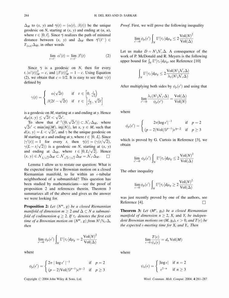
Proposition 2: Let ðNm; gÞ be a closed Riemannian

manifold of dimension m � 2 and � � N a submani-

fold of codimension q � 2. If ��0 denotes the first exit

time of a Brownian motion on ðNm; gÞ from NnN�0�,

then

lim�0!0

�pð�0Þð

N

Ez½��0 �dg ¼ 2VolðNÞ2

Volð�Þ

where

�pð�0Þ ¼2� j log �0 j�1 if p ¼ 2

ðp � 2ÞVolðSp�1Þ�0p�2 if p � 3

(

Proof. First, we will prove the following inequality

lim�0!0

�pð�0Þð

N

Ez½��0 �dg � 2VolðNÞ2

Volð�Þ

Let us make D ¼ NnN ��. A consequence of the

work of P. McDonald and R. Meyers is the following

upper bound forÐ

NEx½��0 �dg, see Reference [10]

ðN

Ez½��0 �dg � 2VolðNnN ��Þ1ðNnN ��Þ

After multiplying both sides by �pð�0Þ and using that

lim�0!0

1ðNnN �0�Þ�pð�0Þ

¼ Volð�ÞVolðNÞ

where

�pð�0Þ ¼2�jlog �0j�1

if p ¼ 2

ðp � 2ÞVolðSp�1Þ�0p�2 if p � 3

(

which is proved by G. Curtois in Reference [3], we

obtain

lim�0!0

�pð�0Þð

N


Volð�Þ

The other inequality

lim�!0

�pð�0Þð

N


Volð�Þ

was just recently proved by one of the authors, see

Reference [4]. &

Theorem 3: Let (Mn, g0) be a closed Riemannian

manifold of dimension n � 2, Xt and Yt be indepen-

dent Brownian motions on (M, g0), � > 0, and Tð�Þ be

the expected �-meeting time for Xt and Yt. Then

lim�!0

Tð�Þ nð�Þ

¼ dn VolðMÞ

where

nð�Þ ¼jlog �j if n ¼ 2

�2�n if n � 3

(



and

dn ¼1

2� if n ¼ 2

2�ðn=2Þðn�2Þð4�Þn=2 if n � 3

8<:

Proof. Let x, y 2 M, and consider two independent

Brownian motions Xt, Yt on ðMn; g0Þ, such that

PðX0 ¼ xÞ ¼ PðY0 ¼ yÞ ¼ 1. If

tx;yð�Þ ¼ infft > 0 j dðXt; YtÞ < �g

then

Tð�Þ ¼ 1

Vol2ðMÞ

ð ðM�M

E½tx;yð�Þ� dg0dg0

Making �0 ¼ �=ffiffiffi2

pin Lemma 1, we will have that two

points x, y2M are �-close if and only if ðx; yÞ 2N �=

ffiffi2

p �M , therefore

tx;yð�Þ ¼ infft > 0 j Zt 2 N �=ffiffi2

p �Mg

where Zt ¼ ðXt; YtÞ; z ¼ ðx; yÞ, and

PðZ0 ¼ zÞ ¼ 1

Since Xt and Yt are independent Brownian motions

on ðM; g0Þ then Zt ¼ ðXt; YtÞ is a Brownian motion

on (N, g)¼ (M�M, g0þ g0) and the above identity

for tx;yð�Þ can be expressed in terms of ��, the first exit

time of a Brownian motion Zt, on N from NnN ��M ,

where PfZ0 ¼ zg ¼ 1

E½tx;yð�Þ� ¼ Ez½��= ffiffi2

p �

As a consequence of this, we have that

Tð�Þ ¼ 1

Vol2ðMÞ

ðM�M

Ez½��= ffiffi2

p � dg

Since �M � N is a submanifold of codimension n

and �0 ¼ �=ffiffiffi2

pwe have that �nð�=

ffiffiffi2

pÞ ¼ 2ð2�n=2Þ=

dn�nð�Þ. Here we have used the identity VolðSn�1Þ¼ 2�ðn=2Þ=�ðn=2Þ. Furthermore, the identities Vol(N)

= Vol(M)2 and Vol(�M)¼ 2n/2 Vol(M) can be easily

obtained using that (N, g)¼ (M�M, g0þ g0) is the

Riemannian product manifold. Putting all these to-

gether and the above result we obtain

lim�!0

Tð�Þ nð�Þ

¼ 2ðn�2Þ=2dn

2 VolðMÞ2n=2

¼ dn VolðMÞ

4. Main Result

In order to achieve the desired throughput, M.

Grossglauser and D. Tse have shown in Reference

[6], the necessity of relaying the data packets; in fact,

the desired throughput can be achieved using only

one relay. They also have shown that any pair of nodes

(i, j) is equally likely, in the limit, to be chosen as a

feasible sender–receiver pair. Therefore, in order to

compute the delay time, per packet, we need only to

do the computation for a randomly chosen pair (i, j).

How close should sender and receiver be? Assume,

for simplicity, that every sender node transmits at the

same power P. Let us focus on the transmission from

node i to j. From Equation (1), it can be seen that

transmission from i to j will be unsuccessful whenever

there is another transmitting interferer ‘, satisfying

jX‘ � Xjj ��

L

� �1=�

jXi � Xjj

Therefore, the best we can do is to restrict transmis-

sions to neighbors, which are at a typical distance of

1=ffiffiffik

p.

Theorem A: Let D(k) be the delay time, per packet, of

a mobile ad hoc wireless network with k nodes lying

on a Torus of unit area. Then D(k)2� (log k). More-

over

limk!1

DðkÞlog k

¼ 1

4�

Proof. By the discussion above we are interested on

finding how Tð1=ffiffiffik

pÞ behaves for k big enough, when

the nodes lie on a at 2-toruszz of unit area. In this case,

we have that Mn ¼ T2 and g0 is the at metric of unit

area on T2. Again by the discussion above, the delay

time DðkÞ, per packet, of a mobile ad hoc wireless

network with k nodes is given by the expected �-meeting time Tð�Þ, of two Brownian motions on the

flat 2-torus, with � ¼ 1=ffiffiffik

p. In particular

limk!1

DðkÞlog k

¼ limk!1

Tð1=ffiffiffik

pÞ

2logffiffiffik

p

zzTheorem 3 shows that this estimate does not depend on theway we choose to get rid of the boundary as long as we endup considering a smooth closed surface without boundary asour domain.



Now using Theorem 3, with n¼ 2 and � ¼ 1=ffiffiffik

pwe

obtain

limk!1

Tð1=ffiffiffik

pÞ

2 logffiffiffik

p ¼ 1

2d2 VolðT2Þ

since VolðT2Þ ¼ 1 and d2 ¼ 1=2�, we obtain

limk!1

DðkÞlog k

¼ 1

4�

5. Simulation Results

We have used Paxson method to approximate Brow-

nian motions [12], and the Mersenne–Twister pseudo

random number generator [9]. Our simulation results

are computed using 1000 runs (to discretize integra-

tion) for 64, 128, 256, 512 and 1024 nodes.

Figure 4 shows how the simulation results approach

the theoretical limit. We have plotted four sets of

simulations. As we decrease the step size, the obtained

delays approaches our limit. The outermost curves are

simply the double and half of the theoretical upper

bound.

6. Conclusions

Advancement in hardware and software technologies

has enabled us to deploy ad hoc networks. Nodes in

an ad hoc network may be mobile and static. It had

been shown that per node throughput of a mobile ad-

hoc network goes to zero as the number of nodes goes

to infinity. Per node throughput does not increase

when nodes can move, but packet exchanges between

source–destination pairs must occur directly. How-

ever, when a packet is exchanged, using at most one

relay, per node throughput increases dramatically to a

constant, as the number of nodes goes to infinity. It has

been stated that this gain in throughput could increase

delay [6]. However, to the best of our knowledge, no

estimate for the expected delay per packet is known.

In this paper, we provide a tight bound for the delay,

we show that delay has logarithmic growth. As con-

sequence we have that mobile ad-hoc wireless net-

works are not scalable for real-time applications.

References

1. Aubin T. A course in differential geometry. In Graduate Studiesin Mathematics, Vol. 27. American Mathematical Society:Providence, Rhode Island, USA, 2001.

2. Chavel I. Eigevalues in Riemannian geometry. In Pure andApplied Mathematics, Vol. 115. Academic Press: Orlando,Florida, USA, 1984.

3. Curtois G. Spectrum of manifolds with holes. Journal ofFunctional Analysis 1995; 134: 194–221.

4. Heberto del Rio. Exit time from manifolds with holes. Preprint.http://www.cs.miami.edu/

5. Manfredo P. Do Carmo. Riemannian Geometry. Birkhauser:Boston, Massachusetts, USA, 1992.

6. Grossglauser M, Tse D. Mobiblity increases the capacity of ad-hoc wireless networks. IEEE/ACM Transactions on Network-ing 2002; 10(4): 477–486.

7. Hsu EP. Stochastic analysis on manifolds. In Graduate Studiesin Mathematics, Vol. 38. American Mathematical Society:Providence, Rhode Island, USA, 2001.

8. Karatzas I, Shreve SE. Brownian motion and stochastic calcu-lus. In Graduate Texts in Mathematics (6th edn), Vol. 113.Springer-Verlag, 2000.

9. Matsumoto M, Nishimura T. Mersenne Twister: a 623- dimen-sionally equidistributed uniform pseudo-random number gen-erator. IEEE/ACM Transactions on Modeling and ComputerSimulation 1998; 8(1): 3–30.

10. McDonald P, Meyers R. Dirichlet spectrum and heat content.Journal of Functional Analysis 2003; 200: 150–159.

11. Miller LE. Distribution of link distances in a wireless network.Journal of Research of the National Institute of Standards andTechnology 2001; 106(2): 401–412.

12. Paxson V. Fast, approximate synthesis of fractional Gaussiannoise for generating self-similar network traffic. ComputerCommunication Review 1997; 27: 5–18.

Fig. 4. Simulation results.



Authors’ Biographies

Heberto del Rio received theLicenciado degree in mathematicsfrom the National University ofMexico, UNAM, in September1993, the M.S. degree in mathe-matics from UNAM, in May 1994,Ph.D. in mathematics from theState University of New York atStony Brook in 1999. FromSeptember 1999 to September2002, he was an assistant professor

of mathematics at CIMAT, Guanajuato, Mexico. He iscurrently seeking the M.S. degree in Computer Sciencefrom the University of Miami, Coral Gables. His researchinterests include Riemannian Geometry, Geometric PDEsand Wireless Networks.

Dilip Sarkar received the B. Tech.(Hons.) degree in electronics andelectrical communication engineer-ing from the Indian Institute ofTechnology, Kharagpur, India, inMay 1983; the M.S. degree in com-puter science from the Indian Insti-tute of Science, Bangalore, India, inDecember 1984 and the Ph.D. incomputer science from the Univer-sity of Central Florida, OR, in May

1988. From January 1985 to August 1986 he was a Ph.D.student at Washington State University, Pullman. He iscurrently an associate professor of Computer Science atthe University of Miami, Coral Gables. His research inter-ests include design and analysis of algorithms, parallel anddistributed processing, the web computing and middleware,multimedia communication over broadband and wirelessnetworks, fuzzy systems, and neural networks. In theseareas, he has guided several theses and has authored numer-ous papers. Dr Sarkar is a senior member of the IEEE, amember of IEEE Communications Society and the Associa-tion for Computing Machinery. He was a recipient of theFourteenth All India Design Competition Award in electro-nics in 1982.



logarithmic expected packet delivery delay in mobile ad hoc wireless networks

Documents