Log Processing Cookbook:A guide to processing ODP conventional logs with Geoframe

5/2004

Any opinions, findings, and conclusions or recommendations expressed in this document are those of the author(s) and do not necessarily reflect the views of the National Science Foundation, Joint Oceanographic Institutions, Inc., or ODP member countries.

- 2 -

Contents

I Introduction ...........................................................................................................................3II Preparing for Log Processing................................................................................................4

A Setting up the Geoframe Project .......................................................................................4B Setting up the Unix directory ............................................................................................6C Obtaining the DLIS files...................................................................................................6D Putting unrecognized logs into the Geoframe catalog........................................................7E Setting up the plotter.........................................................................................................7F The Geoframe Xterm – checking files and the system .......................................................8

III ODP log processing.............................................................................................................9A Process Manager ..............................................................................................................9B Data Load.......................................................................................................................10C Data Manager .................................................................................................................12D WellEdit .........................................................................................................................13E Depth Match (WellEdit)..................................................................................................15F Shift to Sea floor (WellEdit)............................................................................................17G Convert Sonic Slowness to Velocity (Well Edit).............................................................18H PrePlus ...........................................................................................................................19I Data presentation and Log Plots .......................................................................................20

IV Saving and distributing data ................................................................................................24A ASCII Data Save ............................................................................................................24B DLIS Data Save..............................................................................................................28C Archive locations............................................................................................................30D Writing the Processing Notes..........................................................................................30E Data transfer to the ship ..................................................................................................30

Appendicies ..............................................................................................................................31Appendix A. Log curves in Final Logplots ...........................................................................31Appendix B. How to splice curves in Well Edit....................................................................33Appendix C. Standard processing notes document template. ................................................34Appendix D. DSI Shear Sonic information...........................................................................36Appendix E. HNGS processing (internal to the tool) ............................................................37

- 3 -

I IntroductionThe purpose of shore-based log processing is to provide scientists with a comprehensive quality-controlled downhole log data set. This data set can then be used for comparison and integrationwith core and seismic data from each ODP leg: for example the Sagan in-house software is usedto put cores and logs on the same depth scale, and IESX software is used to analyze seismicsections and generate synthetic seismograms from the logs. Shore-based log processingcomprises:- Depth adjustments to remove depth offsets between data from different logging runs

- Corrections specific to certain tools and logs

- Documentation for the logs, with an assessment of log quality

- Conversion of the data to a widely accessible format (ASCII for the conventional logs,GIF for the FMS images and summary diagrams)

- Assembling the data for inclusion in the ODP Logging Services on-line and tapedatabases.

Log analysts at ODP Logging Services carry out the processing, mostly using SchlumbergerGeoQuest’s "GeoFrame" software package. Conventional log data (natural gamma radioactivity,resistivity, density, porosity, sonic velocity, magnetic susceptibility logs) are transmitted viainternet connection from the ship, processed, and returned to the ship, usually within a few daysof logging. Processing of other log data (FMS images, GHMT magnetic polarities, etc.) isgenerally done after the cruise.

- 4 -

II Preparing for Log Processing

A Setting up the Geoframe Project

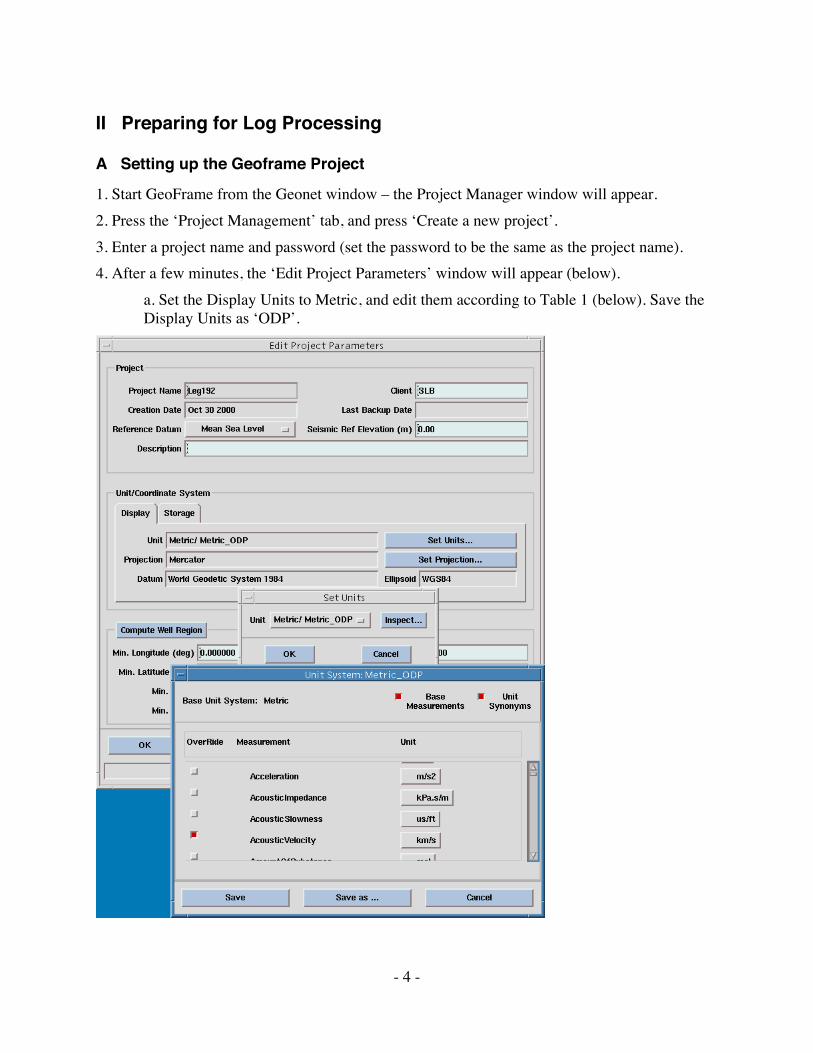
1. Start GeoFrame from the Geonet window – the Project Manager window will appear.2. Press the ‘Project Management’ tab, and press ‘Create a new project’.3. Enter a project name and password (set the password to be the same as the project name).4. After a few minutes, the ‘Edit Project Parameters’ window will appear (below).

a. Set the Display Units to Metric, and edit them according to Table 1 (below). Save theDisplay Units as ‘ODP’.

- 5 -

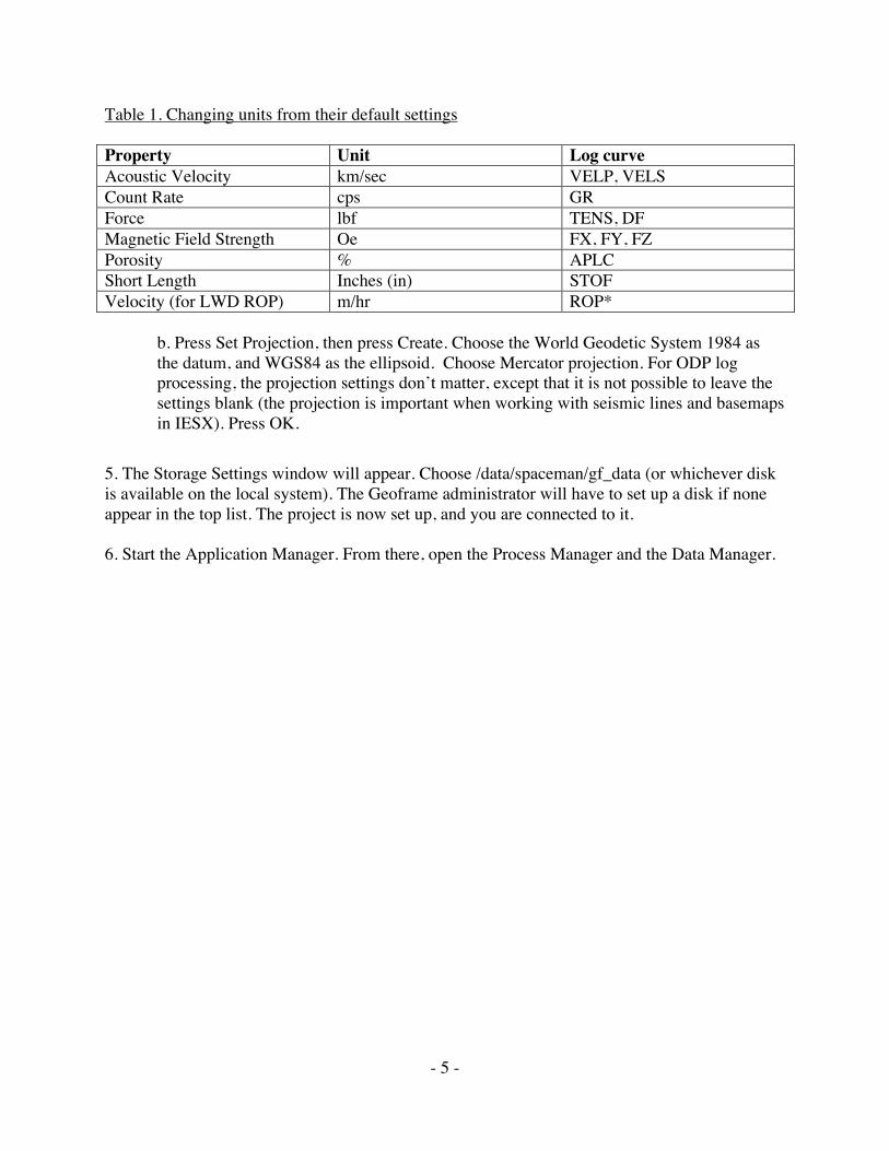
Table 1. Changing units from their default settings

Property Unit Log curveAcoustic Velocity km/sec VELP, VELSCount Rate cps GRForce lbf TENS, DFMagnetic Field Strength Oe FX, FY, FZPorosity % APLCShort Length Inches (in) STOFVelocity (for LWD ROP) m/hr ROP*

b. Press Set Projection, then press Create. Choose the World Geodetic System 1984 asthe datum, and WGS84 as the ellipsoid. Choose Mercator projection. For ODP logprocessing, the projection settings don’t matter, except that it is not possible to leave thesettings blank (the projection is important when working with seismic lines and basemapsin IESX). Press OK.

5. The Storage Settings window will appear. Choose /data/spaceman/gf_data (or whichever diskis available on the local system). The Geoframe administrator will have to set up a disk if noneappear in the top list. The project is now set up, and you are connected to it.

6. Start the Application Manager. From there, open the Process Manager and the Data Manager.

- 6 -

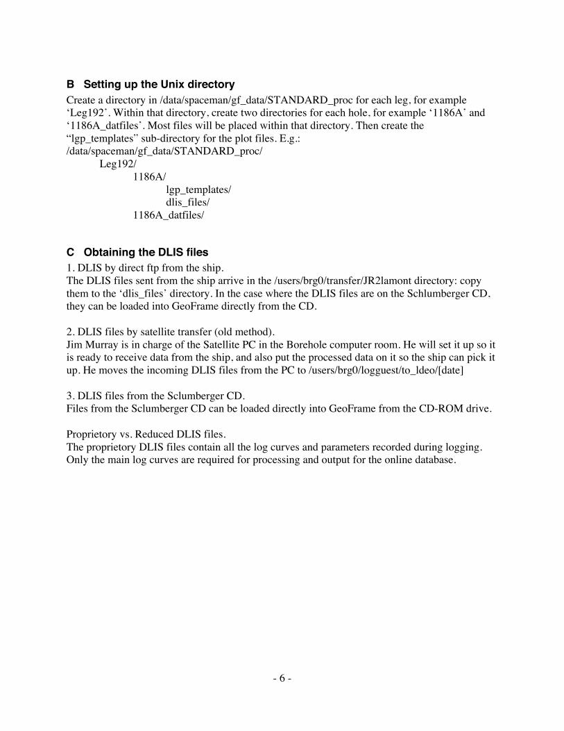
B Setting up the Unix directoryCreate a directory in /data/spaceman/gf_data/STANDARD_proc for each leg, for example‘Leg192’. Within that directory, create two directories for each hole, for example ‘1186A’ and‘1186A_datfiles’. Most files will be placed within that directory. Then create the“lgp_templates” sub-directory for the plot files. E.g.:/data/spaceman/gf_data/STANDARD_proc/

Leg192/1186A/

lgp_templates/dlis_files/

1186A_datfiles/

C Obtaining the DLIS files1. DLIS by direct ftp from the ship.The DLIS files sent from the ship arrive in the /users/brg0/transfer/JR2lamont directory: copythem to the ‘dlis_files’ directory. In the case where the DLIS files are on the Schlumberger CD,they can be loaded into GeoFrame directly from the CD.

2. DLIS files by satellite transfer (old method).Jim Murray is in charge of the Satellite PC in the Borehole computer room. He will set it up so itis ready to receive data from the ship, and also put the processed data on it so the ship can pick itup. He moves the incoming DLIS files from the PC to /users/brg0/logguest/to_ldeo/[date]

3. DLIS files from the Sclumberger CD.Files from the Sclumberger CD can be loaded directly into GeoFrame from the CD-ROM drive.

Proprietory vs. Reduced DLIS files.The proprietory DLIS files contain all the log curves and parameters recorded during logging.Only the main log curves are required for processing and output for the online database.

- 7 -

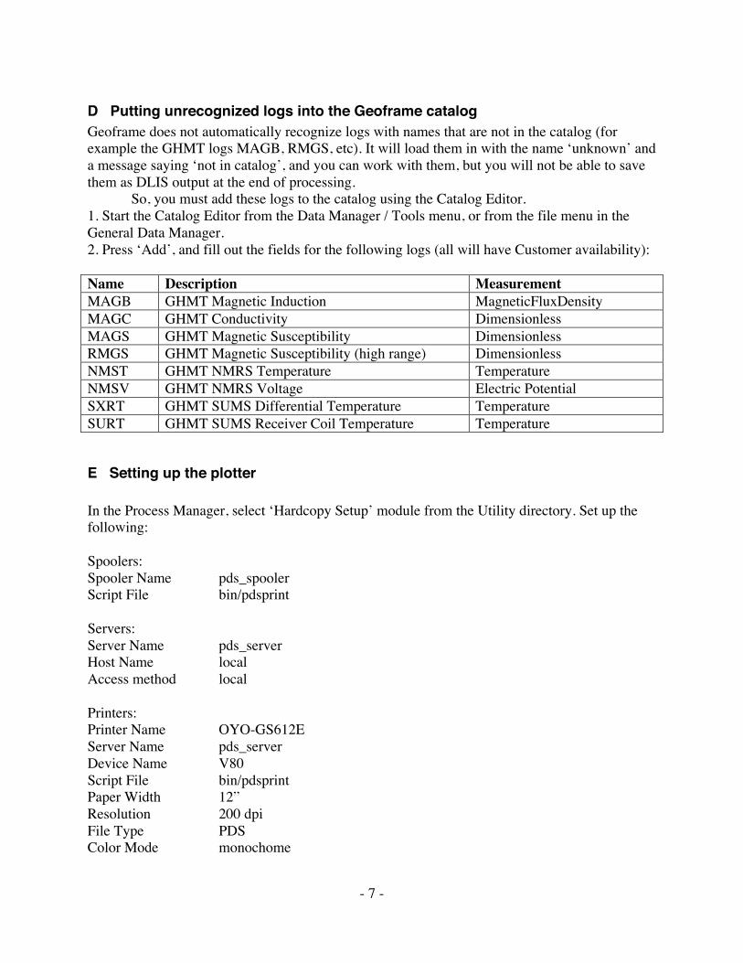
D Putting unrecognized logs into the Geoframe catalogGeoframe does not automatically recognize logs with names that are not in the catalog (forexample the GHMT logs MAGB, RMGS, etc). It will load them in with the name ‘unknown’ anda message saying ‘not in catalog’, and you can work with them, but you will not be able to savethem as DLIS output at the end of processing.

So, you must add these logs to the catalog using the Catalog Editor.1. Start the Catalog Editor from the Data Manager / Tools menu, or from the file menu in theGeneral Data Manager.2. Press ‘Add’, and fill out the fields for the following logs (all will have Customer availability):

Name Description MeasurementMAGB GHMT Magnetic Induction MagneticFluxDensityMAGC GHMT Conductivity DimensionlessMAGS GHMT Magnetic Susceptibility DimensionlessRMGS GHMT Magnetic Susceptibility (high range) DimensionlessNMST GHMT NMRS Temperature TemperatureNMSV GHMT NMRS Voltage Electric PotentialSXRT GHMT SUMS Differential Temperature TemperatureSURT GHMT SUMS Receiver Coil Temperature Temperature

E Setting up the plotter

In the Process Manager, select ‘Hardcopy Setup’ module from the Utility directory. Set up thefollowing:

Spoolers:Spooler Name pds_spoolerScript File bin/pdsprint

Servers:Server Name pds_serverHost Name localAccess method local

Printers:Printer Name OYO-GS612EServer Name pds_serverDevice Name V80Script File bin/pdsprintPaper Width 12”Resolution 200 dpiFile Type PDSColor Mode monochome

- 8 -

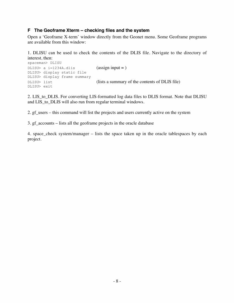
F The Geoframe Xterm – checking files and the systemOpen a ‘Geoframe X-term’ window directly from the Geonet menu. Some Geoframe programsare available from this window:

1. DLISU can be used to check the contents of the DLIS file. Navigate to the directory ofinterest, then:spaceman> DLISU

DLISU> a i=1234A.dlis (assign input = )DLISU> display static fileDLISU> display frame summary

DLISU> list (lists a summary of the contents of DLIS file)DLISU> exit

2. LIS_to_DLIS. For converting LIS-formatted log data files to DLIS format. Note that DLISUand LIS_to_DLIS will also run from regular terminal windows.

2. gf_users – this command will list the projects and users currently active on the system

3. gf_accounts – lists all the geoframe projects in the oracle database

4. space_check system/manager – lists the space taken up in the oracle tablespaces by eachproject.

- 9 -

III ODP log processing

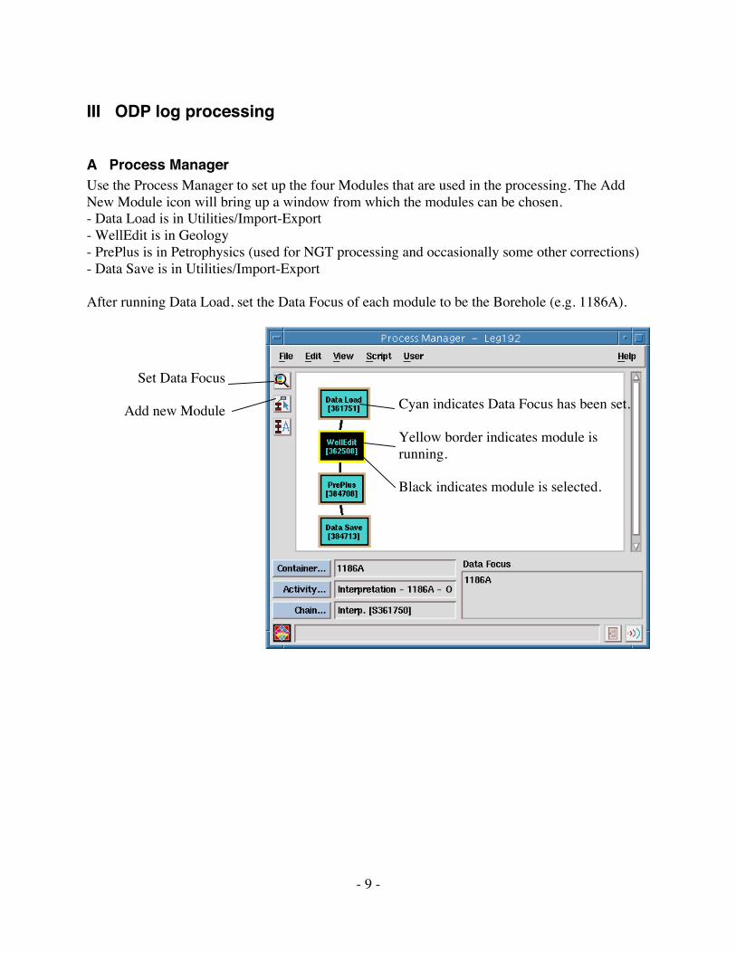
A Process ManagerUse the Process Manager to set up the four Modules that are used in the processing. The AddNew Module icon will bring up a window from which the modules can be chosen.- Data Load is in Utilities/Import-Export- WellEdit is in Geology- PrePlus is in Petrophysics (used for NGT processing and occasionally some other corrections)- Data Save is in Utilities/Import-Export

After running Data Load, set the Data Focus of each module to be the Borehole (e.g. 1186A).

Set Data Focus

Add new Module Cyan indicates Data Focus has been set.

Yellow border indicates module isrunning.

Black indicates module is selected.

- 10 -

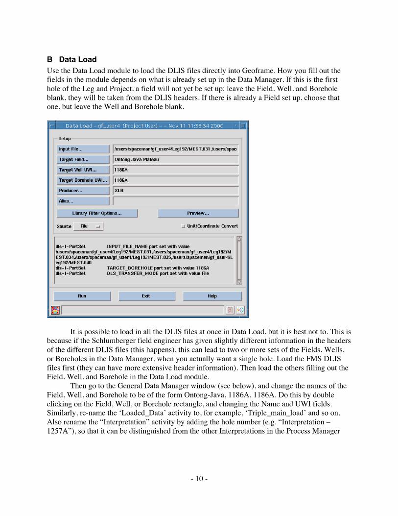
B Data LoadUse the Data Load module to load the DLIS files directly into Geoframe. How you fill out thefields in the module depends on what is already set up in the Data Manager. If this is the firsthole of the Leg and Project, a field will not yet be set up: leave the Field, Well, and Boreholeblank, they will be taken from the DLIS headers. If there is already a Field set up, choose thatone, but leave the Well and Borehole blank.

It is possible to load in all the DLIS files at once in Data Load, but it is best not to. This isbecause if the Schlumberger field engineer has given slightly different information in the headersof the different DLIS files (this happens), this can lead to two or more sets of the Fields, Wells,or Boreholes in the Data Manager, when you actually want a single hole. Load the FMS DLISfiles first (they can have more extensive header information). Then load the others filling out theField, Well, and Borehole in the Data Load module.

Then go to the General Data Manager window (see below), and change the names of theField, Well, and Borehole to be of the form Ontong-Java, 1186A, 1186A. Do this by doubleclicking on the Field, Well, or Borehole rectangle, and changing the Name and UWI fields.Similarly, re-name the ‘Loaded_Data’ activity to, for example, ‘Triple_main_load’ and so on.Also rename the “Interpretation” activity by adding the hole number (e.g. “Interpretation –1257A”), so that it can be distinguished from the other Interpretations in the Process Manager

- 11 -

Proj

ect

F

ield

W

ell

Bor

ehol

e

Act

ivity

S

ervi

ce R

un

Tool

Run

Arra

y (lo

g)

Mod

ule

Run

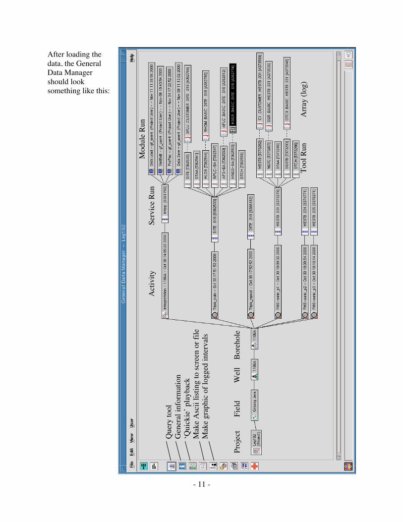
After loading thedata, the GeneralData Managershould looksomething like this:

Que

ry to

olG

ener

al in

form

atio

n‘Q

uick

ie’ p

layb

ack

Mak

e Asc

ii lis

ting

to sc

reen

or f

ileM

ake

grap

hic

of lo

gged

inte

rval

s

- 12 -

C Data ManagerThe Data Manager is used to view and organize all the log data. Logs, parameters, boreholes, etcare generically known as ‘Data Items’

The hierarchy of Data Items in Geoframe goes something like this:Project Field Well Borehole Activity Service Run Tool Run / Module RunLeg 181 SW Pacific 1123B 1123B Data Load Tool String Tool / Module

The Tool Run contains the arrays (logs) (e.g. SGR, POTA, etc) collected by an individuallogging tool (e.g. NGT). The Module Run contains the arrays (logs) that are output by aparticular module (e.g. the BorEID module outputs FMS4.EID).

To navigate around in the General Data Manager, two main tools are useful:

- The menu under MB3 (the right mouse button). Use ‘Expand by’ to prevent gettinghundreds of needless data items on screen, as is possible when you just do ‘Expand’. Use’list arrays’ to list arrays (i.e. logs).

- The ‘Query Tool’ (it’s the crystal ball icon in the left margin of the window). It’s the bestway to find the locations of useful arrays (logs) such as FMS4, *SGR, P1AZ, etc. Selectthe data item under which you want to search (e.g. the Borehole; it will appear blackwhen you click on it). Then in the query tool window, find all ‘Arrays’ with ‘Code’ (thenenter the code, like SGR). Wildcards (*) are acceptable.

Double clicking on any Data Item will bring up a window where the attributes of the DataItem can be examined and edited. Double clicking on an array will produce a sketch of the logdata, a scrollable list of the data values, and the names and modifiers of the log.

- 13 -

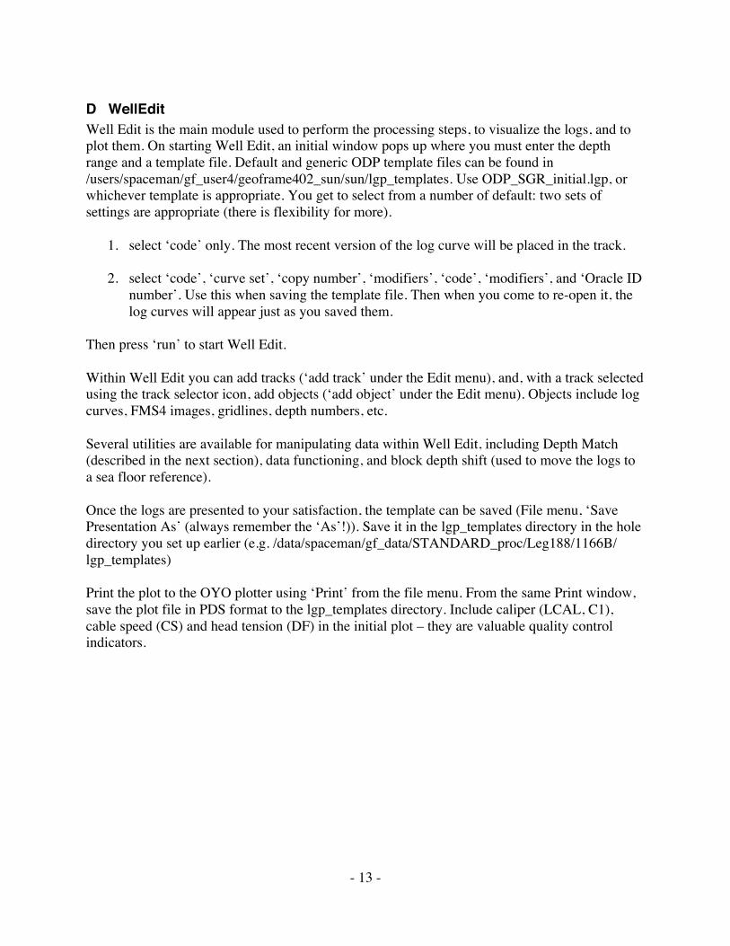
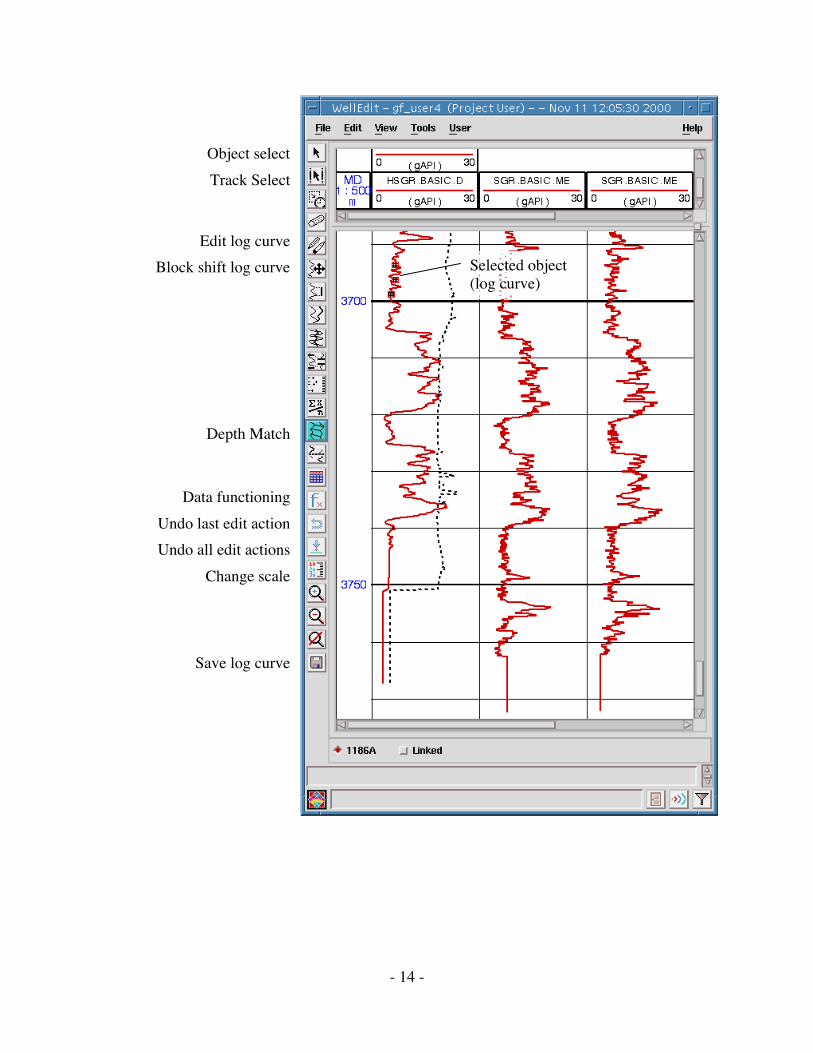
D WellEditWell Edit is the main module used to perform the processing steps, to visualize the logs, and toplot them. On starting Well Edit, an initial window pops up where you must enter the depthrange and a template file. Default and generic ODP template files can be found in/users/spaceman/gf_user4/geoframe402_sun/sun/lgp_templates. Use ODP_SGR_initial.lgp, orwhichever template is appropriate. You get to select from a number of default: two sets ofsettings are appropriate (there is flexibility for more).

1. select ‘code’ only. The most recent version of the log curve will be placed in the track.

2. select ‘code’, ‘curve set’, ‘copy number’, ‘modifiers’, ‘code’, ‘modifiers’, and ‘Oracle IDnumber’. Use this when saving the template file. Then when you come to re-open it, thelog curves will appear just as you saved them.

Then press ‘run’ to start Well Edit.

Within Well Edit you can add tracks (‘add track’ under the Edit menu), and, with a track selectedusing the track selector icon, add objects (‘add object’ under the Edit menu). Objects include logcurves, FMS4 images, gridlines, depth numbers, etc.

Several utilities are available for manipulating data within Well Edit, including Depth Match(described in the next section), data functioning, and block depth shift (used to move the logs toa sea floor reference).

Once the logs are presented to your satisfaction, the template can be saved (File menu, ‘SavePresentation As’ (always remember the ‘As’!)). Save it in the lgp_templates directory in the holedirectory you set up earlier (e.g. /data/spaceman/gf_data/STANDARD_proc/Leg188/1166B/lgp_templates)

Print the plot to the OYO plotter using ‘Print’ from the file menu. From the same Print window,save the plot file in PDS format to the lgp_templates directory. Include caliper (LCAL, C1),cable speed (CS) and head tension (DF) in the initial plot – they are valuable quality controlindicators.

- 14 -

Object selectTrack Select

Edit log curveBlock shift log curve

Depth Match

Data functioningUndo last edit actionUndo all edit actions

Change scale

Save log curve

Selected object(log curve)

- 15 -

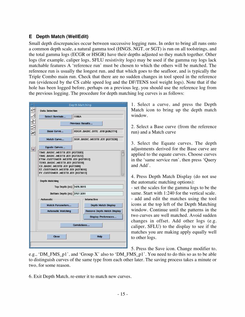
E Depth Match (WellEdit)Small depth discrepancies occur between successive logging runs. In order to bring all runs ontoa common depth scale, a natural gamma tool (HNGS, NGT, or SGT) is run on all toolstrings, andthe total gamma logs (ECGR or HSGR) have their depths adjusted so they match together. Otherlogs (for example, caliper logs, SFLU resistivity logs) may be used if the gamma ray logs lackmatchable features A ‘reference run’ must be chosen to which the others will be matched. Thereference run is usually the longest run, and that which goes to the seafloor, and is typically theTriple Combo main run. Check that there are no sudden changes in tool speed in the referencerun (evidenced by the CS cable speed log and the DF/TENS tool weight logs). Note that if thehole has been logged before, perhaps on a previous leg, you should use the reference log fromthe previous logging. The procedure for depth matching log curves is as follows:

1. Select a curve, and press the DepthMatch icon to bring up the depth matchwindow.

2. Select a Base curve (from the referencerun) and a Match curve

3. Select the Equate curves. The depthadjustments derived for the Base curve areapplied to the equate curves. Choose curvesin the ‘same service run’, then press ‘Queryand Add’.

4. Press Depth Match Display (do not usethe automatic matching options):- set the scales for the gamma logs to be thesame. Start with 1:240 for the vertical scale.- add and edit the matches using the toolicons at the top left of the Depth Matchingwindow. Continue until the patterns in thetwo curves are well matched. Avoid suddenchanges in offset. Add other logs (e.g.caliper, SFLU) to the display to see if thematches you are making apply equally wellto other logs.

5. Press the Save icon. Change modifier to,e.g., ‘DM_FMS_p1’, and ‘Group X’ also to ‘DM_FMS_p1’. You need to do this so as to be ableto distinguish curves of the same type from each other later. The saving process takes a minute ortwo, for some reason.

6. Exit Depth Match, re-enter it to match new curves.

- 16 -

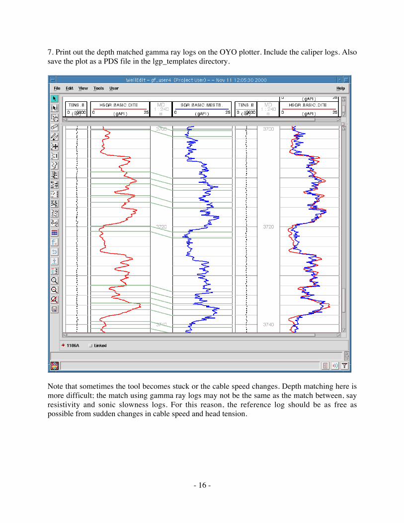
7. Print out the depth matched gamma ray logs on the OYO plotter. Include the caliper logs. Alsosave the plot as a PDS file in the lgp_templates directory.

Note that sometimes the tool becomes stuck or the cable speed changes. Depth matching here ismore difficult; the match using gamma ray logs may not be the same as the match between, sayresistivity and sonic slowness logs. For this reason, the reference log should be as free aspossible from sudden changes in cable speed and head tension.

- 17 -

F Shift to Sea floor (WellEdit)Initially, the logs are on depth scales referenced to the rig floor (metres below rig floor, mbrf).The sea floor appears in the natural gamma log as a step to lower background values in the watercolumn above the sea floor. We shift the reference to sea floor (metres below sea floor, mbsf) bysubtracting natural gamma seafloor depth (mbrf) from all the log depths. This is done in WellEdit:

- Display the natural gamma curve at the seafloor and choose the sea floor depth near thebase of the step decrease in that log, using the driller’s seafloor depth as a guide.Sometimes the natural gamma logs do not cross the sea floor. In this case, generally, thedriller’s sea floor depth is used.

- Select the HSGR/SGR curve in WellEdit, and press the Block Depth Shift icon.

- Enter the vertical shift in the Depth Shift window (a negative number). Press Update andthen Close.

- Press the ‘Save’ icon. Press ‘Propagate To’, then ‘Add Curves’, and set the array code to‘*’; set the Data Focus to the Activity ‘Triple_main’ (or whichever is the reference run),set the curve to ‘*’, and press ‘Add.’ Check that all the required curves are present in thelist. In the case of Depth Matched data, select ‘Add curves in Same Container’, then press‘Query and Add’

- Change the Modifier to ‘DSH_Triple_main.’

- Press OK. The process of saving the shifted curves can take a minute.

- N.B. Remember to change the activity name from WellEdit to ‘DSH_Triple_main’ in theGeneral Data Manager. If you don’t, the depth shifted curves from the next toolstring willend up in the same activity.

- Repeat for the other passes.

TipsIf the seafloor is not clear, display the component gamma logs (K, Th, U). Trust the K more thanU. Also compare the driller’s depth to the base of the pipe to the log depth to the base of thepipe, to see if the difference is similar to the difference at seafloor.

- 18 -

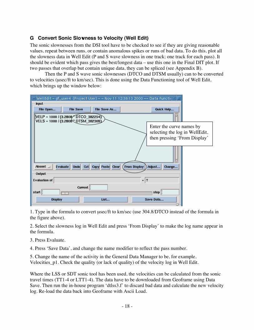
G Convert Sonic Slowness to Velocity (Well Edit)The sonic slownesses from the DSI tool have to be checked to see if they are giving reasonablevalues, repeat between runs, or contain anomalous spikes or runs of bad data. To do this, plot allthe slowness data in Well Edit (P and S wave slowness in one track; one track for each pass). Itshould be evident which pass gives the best/longest data – use this one in the Final DIT plot. Iftwo passes that overlap but contain unique data, they can be spliced (see Appendix B).

Then the P and S wave sonic slownesses (DTCO and DTSM usually) can to be convertedto velocities (µsec/ft to km/sec). This is done using the Data Functioning tool of Well Edit,which brings up the window below:

1. Type in the formula to convert µsec/ft to km/sec (use 304.8/DTCO instead of the formula inthe figure above).2. Select the slowness log in Well Edit and press ‘From Display’ to make the log name appear inthe formula.3. Press Evaluate.4. Press ‘Save Data’, and change the name modifier to reflect the pass number.5. Change the name of the activity in the General Data Manager to be, for example,Velocities_p1. Check the quality (or lack of quality) of the velocity log in Well Edit.

Where the LSS or SDT sonic tool has been used, the velocities can be calculated from the sonictravel times (TT1-4 or LTT1-4). The data have to be downloaded from Geoframe using DataSave. Then run the in-house program ‘dtlss3.f’ to discard bad data and calculate the new velocitylog. Re-load the data back into Geoframe with Ascii Load.

Enter the curve names byselecting the log in WellEdit,then pressing ‘From Display’

- 19 -

H PrePlusPre Plus is a powerful module used to correct the NGT logs for borehole diameter and thedensity of the drilling fluid. Since the NGT is no longer used in ODP, we do not go into thedetails of the Pre Plus module here. Pre Plus can be used to make borehole size, temperature, andother corrections to many tools and log types.

Comparison of the all the HNGS and NGT runs is a good idea, to test repeatability. Total gammausually repeats quite well, but Thorium and especially Uranium can be way different. Take alook.

- 20 -

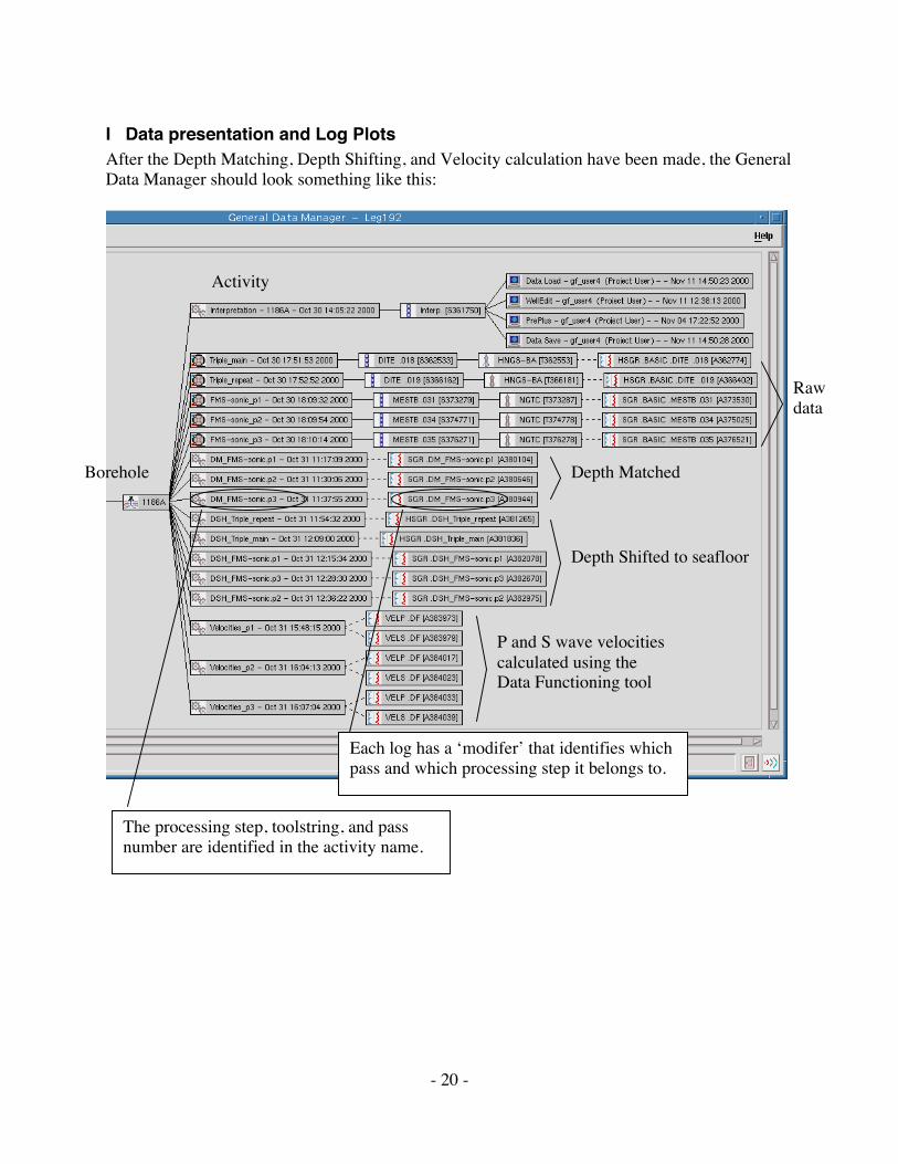
I Data presentation and Log PlotsAfter the Depth Matching, Depth Shifting, and Velocity calculation have been made, the GeneralData Manager should look something like this:

Depth Matched

Depth Shifted to seafloor

Borehole

Activity

P and S wave velocitiescalculated using theData Functioning tool

Rawdata

Each log has a ‘modifer’ that identifies whichpass and which processing step it belongs to.

The processing step, toolstring, and passnumber are identified in the activity name.

- 21 -

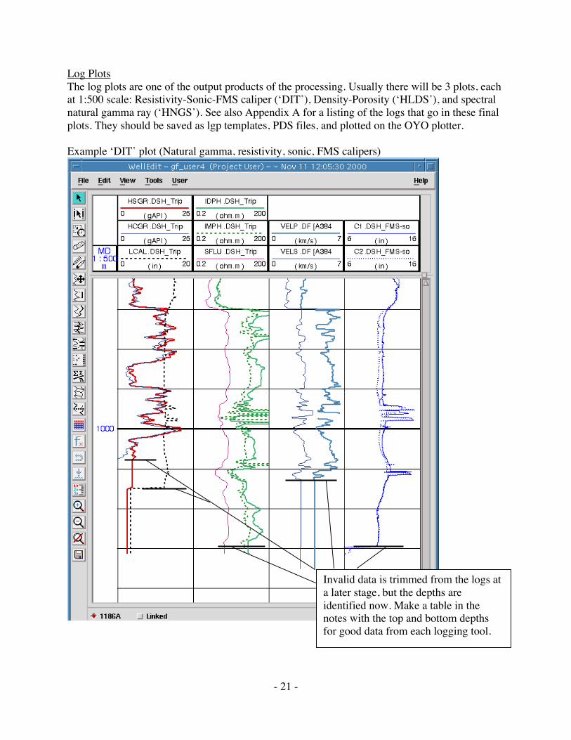
Log PlotsThe log plots are one of the output products of the processing. Usually there will be 3 plots, eachat 1:500 scale: Resistivity-Sonic-FMS caliper (‘DIT’), Density-Porosity (‘HLDS’), and spectralnatural gamma ray (‘HNGS’). See also Appendix A for a listing of the logs that go in these finalplots. They should be saved as lgp templates, PDS files, and plotted on the OYO plotter.

Example ‘DIT’ plot (Natural gamma, resistivity, sonic, FMS calipers)

Invalid data is trimmed from the logs ata later stage, but the depths areidentified now. Make a table in thenotes with the top and bottom depthsfor good data from each logging tool.

- 22 -

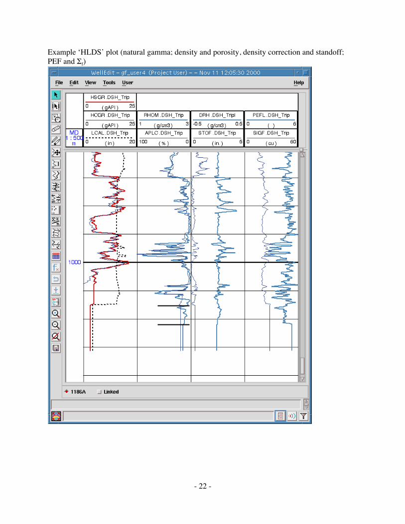
Example ‘HLDS’ plot (natural gamma; density and porosity, density correction and standoff;PEF and Σf)

- 23 -

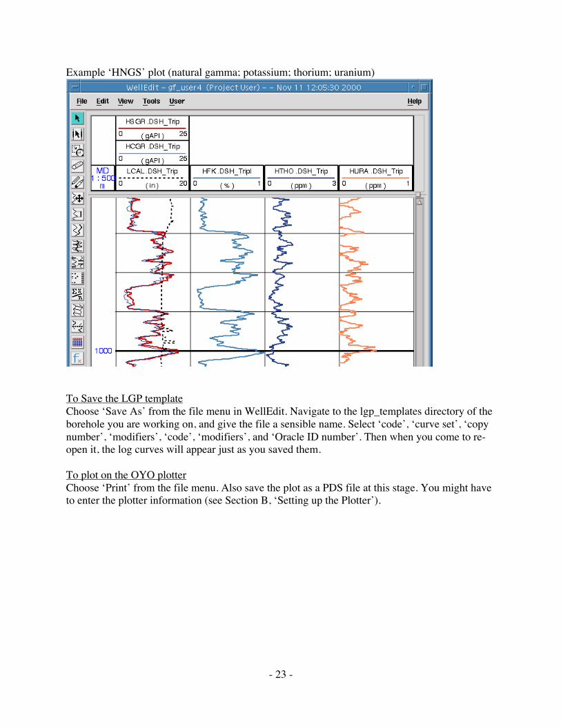
Example ‘HNGS’ plot (natural gamma; potassium; thorium; uranium)

To Save the LGP templateChoose ‘Save As’ from the file menu in WellEdit. Navigate to the lgp_templates directory of theborehole you are working on, and give the file a sensible name. Select ‘code’, ‘curve set’, ‘copynumber’, ‘modifiers’, ‘code’, ‘modifiers’, and ‘Oracle ID number’. Then when you come to re-open it, the log curves will appear just as you saved them.

To plot on the OYO plotterChoose ‘Print’ from the file menu. Also save the plot as a PDS file at this stage. You might haveto enter the plotter information (see Section B, ‘Setting up the Plotter’).

- 24 -

IV Saving and distributing data

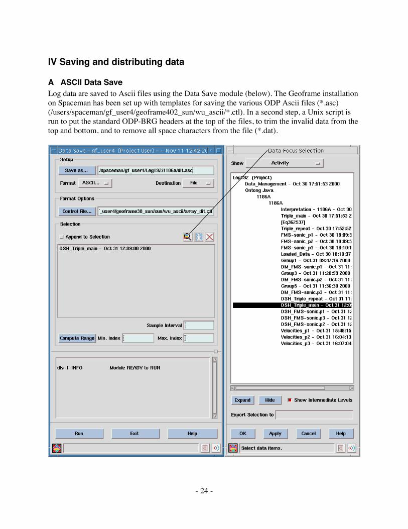
A ASCII Data SaveLog data are saved to Ascii files using the Data Save module (below). The Geoframe installationon Spaceman has been set up with templates for saving the various ODP Ascii files (*.asc)(/users/spaceman/gf_user4/geoframe402_sun/wu_ascii/*.ctl). In a second step, a Unix script isrun to put the standard ODP-BRG headers at the top of the files, to trim the invalid data from thetop and bottom, and to remove all space characters from the file (*.dat).

- 25 -

- In the Data Save module, set the format to Ascii, and a drop-down menu should list theSave Templates (array_dit.ctl, array_hlds.ctl, etc). Choose the top one and work down thelist, as appropriate for the tool strings used in the hole. The control file will appear in theControl File box.

- Press ‘Save As’, navigate to the Hole directory, and set the filename to be of the form‘ditm.asc’ (i.e. with the tool first, the pass second). The naming convention is that the toolname is followed by a letter or number indicating the pass, e.g. m for Main, 1 for Pass 1,u for Upper Pass, etc.

- Set ‘Destination’ to ‘File’

- Press the Data Focus icon and navigate down so that all Activities in the Borehole aredisplayed (see figure below). Select the Activity containing the relevant data (e.g.DSH_Triple_main for ditm.asc), and press Apply. Include the velocity data with the DSIslownesses. For the processed NGT curves, you have to select the appropriate ModuleRun of the Pre-Plus module in the Interpretation Chain (see the DLIS Save figure).

- Leave the Sample Interval and Compute Range blank, except for the GPIT and FMScaliper file, where you have to set the sample interval to 0.1524 m.

- Press Run.

- Repeat for all other tools on all passes of the toolstrings.

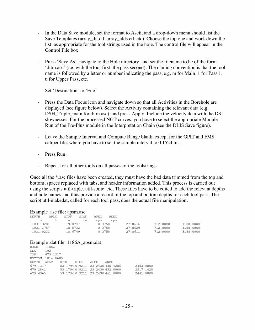
Once all the *.asc files have been created, they must have the bad data trimmed from the top andbottom, spaces replaced with tabs, and header information added. This process is carried outusing the scripts util-triple, util-sonic, etc. These files have to be edited to add the relevant depthsand hole names and thus provide a record of the top and bottom depths for each tool pass. Thescript util-makedat, called for each tool pass, does the actual file manipulation.

Example .asc file: apsm.ascDEPTH APLC STOF SIGF AFEC ANEC m % in. cu cps cps 1031.3281 19.0747 0.3750 27.8646 712.0000 3188.0000 1031.1757 18.8732 0.3750 27.8629 712.0000 3188.0000 1031.0233 18.6749 0.3750 27.8611 712.0000 3188.0000

Example .dat file: 1186A_apsm.datHOLE: 1186ALEG: 192TOP: 679.1317BOTTOM: 1014.8689DEPTH APLC STOF SIGF AFEC ANEC679.1317 53.1794 0.9211 23.2430 435.4286 2483.0000679.2841 53.1794 0.9211 23.2430 432.0000 2517.1428679.4365 53.1794 0.9211 23.2430 461.0000 2441.0000

- 26 -

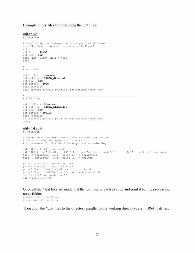
Example utility files for producing the .dat files:

util-triple#! /bin/csh

# Shell Script to re-format ascii output from GeoFrameecho 'Re-formatting ascii output from GeoFrame'echoset hole = 1186Aset leg = 192echo 'Leg '$leg' Hole '$holeecho

# ________________________________________________________________________# DIT file

set infile = ditm.ascset outfile = 1186A_ditm.datset top = 679set bottom = 1030echo $outfileutil-makedat $infile $outfile $top $bottom $hole $leg

# ________________________________________________________________________# HLDS file

set infile = hldsm.ascset outfile = 1186A_hldsm.datset top = 679set bottom = 1021.5echo $outfileutil-makedat $infile $outfile $top $bottom $hole $leg[etc]

util-makedat#! /bin/csh

# Script to do the re-format of the Geoframe ascii output.# Called from util-triple, etc, like this:# util-makedat $infile $outfile $top $bottom $hole $leg

awk 'NR == 1' $1 > tmp.headerawk '($1 <= '$4' && $1 >= '$3')' $1 | sed 's/ //g' | sed ‘s/ $//g’ | sort -n > tmp.bogustail -1 tmp.bogus | awk '{print $1}' > tmp.bottomhead -1 tmp.bogus | awk '{print $1}' > tmp.top

printf '%s\t%s\n' "HOLE:" $5 > $2printf '%s\t%s\n' "LEG:" $6 >> $2printf '%s\t' "TOP:" >> $2; cat tmp.top >> $2printf '%s\t' "BOTTOM:" >> $2; cat tmp.bottom >> $2sed 's/ //g' tmp.header >> $2cat tmp.bogus >> $2

Once all the *.dat files are made, list the top lines of each to a file and print it for the processingnotes folder:> head *.dat > datfiles> enscript –2r datfiles

Then copy the *.dat files to the directory parallel to the working directory, e.g. 1186A_datfiles.

- 27 -

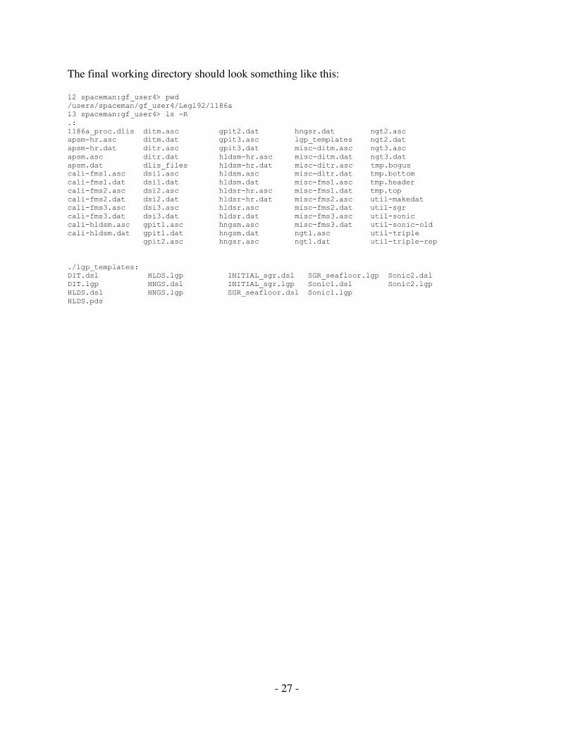
The final working directory should look something like this:

12 spaceman:gf_user4> pwd/users/spaceman/gf_user4/Leg192/1186a13 spaceman:gf_user4> ls -R.:1186a_proc.dlis ditm.asc gpit2.dat hngsr.dat ngt2.ascapsm-hr.asc ditm.dat gpit3.asc lgp_templates ngt2.datapsm-hr.dat ditr.asc gpit3.dat misc-ditm.asc ngt3.ascapsm.asc ditr.dat hldsm-hr.asc misc-ditm.dat ngt3.datapsm.dat dlis_files hldsm-hr.dat misc-ditr.asc tmp.boguscali-fms1.asc dsi1.asc hldsm.asc misc-ditr.dat tmp.bottomcali-fms1.dat dsi1.dat hldsm.dat misc-fms1.asc tmp.headercali-fms2.asc dsi2.asc hldsr-hr.asc misc-fms1.dat tmp.topcali-fms2.dat dsi2.dat hldsr-hr.dat misc-fms2.asc util-makedatcali-fms3.asc dsi3.asc hldsr.asc misc-fms2.dat util-sgrcali-fms3.dat dsi3.dat hldsr.dat misc-fms3.asc util-soniccali-hldsm.asc gpit1.asc hngsm.asc misc-fms3.dat util-sonic-oldcali-hldsm.dat gpit1.dat hngsm.dat ngt1.asc util-triple gpit2.asc hngsr.asc ngt1.dat util-triple-rep

./lgp_templates:DIT.dsl HLDS.lgp INITIAL_sgr.dsl SGR_seafloor.lgp Sonic2.dslDIT.lgp HNGS.dsl INITIAL_sgr.lgp Sonic1.dsl Sonic2.lgpHLDS.dsl HNGS.lgp SGR_seafloor.dsl Sonic1.lgpHLDS.pds

- 28 -

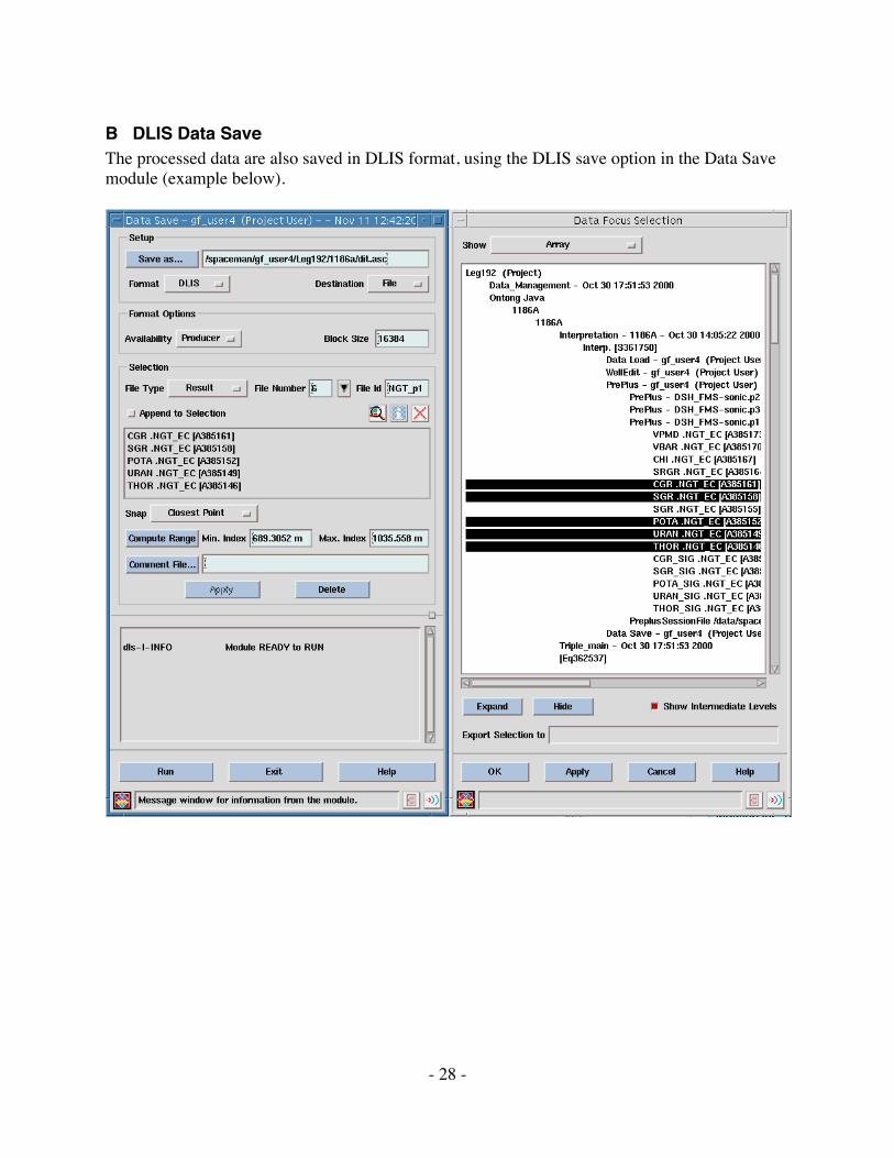
B DLIS Data SaveThe processed data are also saved in DLIS format, using the DLIS save option in the Data Savemodule (example below).

- 29 -

Procedure for saving in DLIS format:

1. Select DLIS, File/Tape, and the output path and filename.2. Select ‘producer’ for availability.3. Leave the default blocksize.4. Use the data focus icon to select the data items to save:

a. Expand from the field level down through the well and borehole to get a list of theactivities within the borehole.b. For the triple combo, select (for example) the DSH_triple_main activity, and press Apply.The activity will appear in the box, and the file number (the logical file number) will updateautomatically.c. Sometimes you need to select individual arrays, for example where NGT arrays have beenreprocessed:

i. Select the Pre-Plus Module Run. Press Apply (in the data focus window).ii. Toggle the ‘append to selection’ option.iii. Using MB3, list the arrays within the DSH activity. Select all but the NGT arrays(you can drag select, and use the control key to deselect). Press Apply.iv. Select the Activity containing the P and S wave velocities. Press Apply.

5. Set the file type to Result.6. Set the file ID to Triple_main, GHMT_p1, etc.7. Set the snap option to ‘off’.8. You don’t need to Compute Range.9. Press Apply. NB none of the above settings are applied until you do this.10. Return to step 4 and select the next set of data items to be saved. Each pass will have aseparate logical file.

- 30 -

C Archive locationsThe processed data in Ascii format are maintained in several locations:- Where they were processed (/data/spaceman/gf_data/STANDARD_proc)- In the Ascii database on Cristina Broglia’s Mac.- In the online database, /data/web_brg0/WWW_BRG/online2- On CD-ROM.

The DLIS processed data are maintained in the archive:- /data/web_brg0/WWW_BRG/archive/ODP_data_proc/standard- On 4mm DAT tape.

D Writing the Processing NotesSee document template in Appendix C.In the DSDP processing notes, written after ODP processing was finished, we have introduced atable with the logging tool strings and depth ranges, which should be continued in future IODPlog processing. For example:

Tool string Pass Topdepth(mbsf)

Bottomdepth(mbsf)

Bit depth(mbsf)

Notes

1. DIT/LSS/GR/MCD Main 150 536 1712. FDC/CNL/GR Main 0 530 172 Reference

Repeat 441.5 492

E Data transfer to the shipPut the processed and zipped Ascii files to be sent to the ship in the outgoing directory(/users/brg0/transfer/lamont2JR/Leg/Hole). Let the Logging Staff Scientist onboard the shipknow the data have been processed and are ready to be picked up. The data will be picked up bythe Logging Staff Scientist.

- 31 -

Appendicies

Appendix A. Log curves in Final Logplots

Wireline

Template #1: Resistivity-Spectral Gamma Ray-Sonic-FMS CalipersTrack 1: Spectral Gamma ray: HSGR (or SGR), HCGR (or CGR), API unitsTrack 2: Resistivity: IDPH, IMPH, SFLU (ohmm), linear or logarithmicTrack 3: Sonic: compressional velocity (Long and short-spacing, km/s)OrTrack 3: Sonic: compressional and shear velocity (km/s)Track 4: FMS calipers (in)

Template #2: Resistivity- Spectral Gamma Ray-Sonic-HLDT caliperTrack 1: Spectral Gamma ray: HSGR (or SGR), HCGR (or CGR), API units, HLDT caliper (in)Track 2: Resistivity: IDPH, IMPH, SFLU (ohmm), linear or logarithmicTrack 3: Sonic: compressional velocity (Long and short-spacing, km/s)Track 4: Spectral Gamma Ray: HTHO (or THOR) and HURA (or URAN, both ppm), HFK (orPOTA, wt %)

Template #3: Spectral Gamma Ray-Density-Porosity-HLDT CaliperTrack 1: Spectral Gamma ray: HSGR (or SGR), HCGR (or CGR), API units, HLDT caliper (in)Track 2: Bulk Density (g/cm3), Porosity (%)Track 3: Density Correction (g/cm3), Standoff (in)Track 4: Capture cross section (capture units), Photoelectric Effect (barns/e-)

Template #4: Spectral Gamma RayTrack 1: Spectral Gamma ray: HSGR (or SGR), HCGR (or CGR), API units, HLDT caliper (in)Track 2: HFK (or POTA, wt %)Track 3: HTHO (or THOR, ppm)Track 4: HURA (or URAN, ppm)

NOTE: if you choose template #2, there is no need for template #4.

LWD

Template #1: Penetration Rate-Gamma Ray-Resistivity-Spectral Gamma RayTrack 1: Gamma ray: GR (API units), ROP (f/hr)Track 2: Resistivity: ATR and PSR (ohmm), linear or logarithmicTrack 3: Spectral Gamma Ray (SGR and CGR, API units)Track 4: Spectral Gamma Ray: THOR and URAN (ppm), POTA (wt %)

- 32 -

Template #2: Penetration Rate-Spectral Gamma Ray-ResistivityTrack 1: Spectral Gamma ray: GR (API units), ROP (f/hr)Track 2: Resistivity: ATR and PSR (ohmm), linear or logarithmicTrack 3: Spectral Gamma ray POTA (wt %)Track 4: Spectral Gamma Ray: THOR and URAN (ppm)

Template #3: Spectral Gamma Ray-Density-Porosity- CaliperTrack 1: Spectral Gamma ray: SGR and CGR), API units, caliper (in)Track 2: Bulk Density (g/cm3), Porosity (%)Track 3: Density Correction (g/cm3), Photoelectric Effect (barns/e-)Track 4: Spectral Gamma Ray: THOR and URAN (ppm), POTA (wt %)

- 33 -

Appendix B. How to splice curves in Well Edit

Description:This example will describe the case where you want to splice two arrays with the same codefrom different service runs, for example, two sp curves from a shallow and a deep log run.

Solution:After starting WellEdit, click on the Splice Multiple Log Curves Simultaneously icon, thetwelvth icon from the top. This brings up the Splice Mode window. Select the boreholecontaining the curves you wish to splice. Next, Select the Activities which contain the arrays youwish to splice. In this case, it is not necessary to Customize Splice Groups. Each activity will begiven a Group Name which is the same as the activity name and the Group Focus will be set tothat activity.

Next, click the Use Common Codes button. This will show the arrays which are common to allthe Groups (or Activities) which have been selected. The Display Log Curve will have the codeof one of the arrays available to be spliced. You can change this by highlighting a different arrayand typing in the code for the Display Log Curve. The Display Log Curve input will determinewhich curves will be displayed.

Next, click Splice Display. This will bring up a WellEdit window that shows each array with thecommon code in an individual log track, with an output track to the right which shows thespliced curve. You may need to expand or scroll this window to see all tracks. The Splice iconsare those four icons back in the Splice Mode window, so position this window where you can usethose icons and still see the Splice Display window.

The next step is to put in the splice point(s) by clicking on the top icon in Splice Mode, thenmoving to the WellEdit window and clicking on the log at the splice point. A green line willappear across all log tracks. To remove a splice point, click on the second icon then click on thegreen line. To select the log interval to be spliced, click on the third icon, then click on thedesired track anywhere above the green line. Then click on a different track below the green line.The output window will now show the spliced version of the log. Continue putting in splicepoints and selecting the log intervals. When finished splicing, click on the save icon in theWellEdit window to save the spliced log.

GeoQuest Custumer Support Knowledge Base, 12/21/98

- 34 -

Appendix C. Standard processing notes document template.

ODP logging contractor: LDEO-BRGHole:Leg:Location:Latitude: ° 'Longitude: ° 'Logging date:Bottom felt: mbrf (used for depth shift to sea floor)Total penetration: mbsfTotal core recovered: m ( %)

Logging Runs

Logging string 1:Logging string 2:Logging string 3:

Text explaining notable events in the logging operations, ship heave conditions, and whether thewireline heave compensator was used.

Bottom-hole Assembly/Pipe/Casing

The following bottom-hole assembly/pipe/casing depths are as they appear on the logs afterdifferential depth shift (see “Depth shift” section) and depth shift to the sea floor. As such, theremight be a discrepancy with the original depths given by the drillers onboard. Possible reasonsfor depth discrepancies are ship heave, use of wireline heave compensator, and drill string and/orwireline stretch.DIT/APS/HLDT/HNGS: Bottom-hole assembly at mbsfFMS/DSI/GPIT/SGT: Bottom-hole assembly at mbsf.

Processing

Depth shift: The original logs were depth matched to the HNGS/NGT from the ………… runand were then shifted to the sea floor (-m). The sea floor depth is determined by the step ingamma ray values at the sediment-water interface. In this case it is the same as the "bottom felt"depth given by the drillers (see above).Depth matching is typically done in the following way. One log is chosen as reference (base) log(usually the total gamma ray log from the run with the greatest vertical extent), and then thefeatures in the equivalent logs from the other runs are matched to it in turn. This matching isperformed automatically, and the result checked and adjusted as necessary. The depthadjustments that were required to bring the match log in line with the base log are then applied toall the other logs from the same tool string.

- 35 -

Gamma-ray processing: The HNGS and SGT data were corrected for hole size during therecording.

Acoustic data processing: Because of the extremely noisy character of the sonic logs, noprocessing has been performed at this stage.

Acoustic data processing: The array sonic tool was operated in two modes: linear array mode,with the 8-receivers providing full waveform analysis (compressional and shear) and standarddepth-derived borehole compensated mode, including long-spacing (8-10-10-12') and short-spacing (3-5-5-7') logs. The sonic logs have been processed to eliminate some of the noise andcycle skipping experienced during the recording. Using two sets of the four transit timemeasurements and proper depth justification, four independent measurements over a -2ft intervalcentered on the depth of interest are determined, each based on the difference between a pair oftransmitters and receivers. The program discards any transit time that is negative or falls outsidea range of meaningful values selected by the processor.

High-resolution data: Bulk density and neutron porosity data were recorded at a sampling rateof 2.54 and 5.08 cm, respectively. SGT gamma ray data were sampled every 5.08 cm. Theenhanced bulk density curve is the result of Schlumberger enhanced processing techniqueperformed on the MAXIS system onboard. While in normal processing short-spacing data issmoothed to match the long-spacing one, in enhanced processing this is reversed. In a situationwhere there is good contact between the HLDT/HLDS pad and the borehole wall (low-densitycorrection) the results are improved, because the short spacing has better vertical resolution.

Quality Control

null value=-999.25. This value may replace invalid log values or results. During the processing, quality control of the data is mainly performed by cross-correlation of alllogging data. Large (>12") and/or irregular borehole affects most recordings, particularly thosethat require eccentralization (APS, HLDT/HLDS) and a good contact with the borehole wall.Hole deviation can also affect the data negatively; the FMS, for example, is not designed to berun in holes deviated more than 10 degrees, as the tool weight might cause the caliper to close.Data recorded through bottom-hole assembly should be used qualitatively only because of theattenuation on the incoming signal.Hole diameter was recorded by the hydraulic caliper on the HLDT/HLDS tool (CALI/LCAL)and on the FMS string (C1 and C2).

Additional information about the logs can be found in the “Explanatory Notes” and Site Chapter,ODP IR volume ….. For further questions about the logs, please contact:

Trevor WilliamsPhone: 845-365-8626Fax: 845-365-3182E-mail: trevor@ldeo.columbia.edu

Cristina Broglia

- 36 -

Phone: 845-365-8343Fax: 845-365-3182E-mail: chris@ldeo.columbia.edu

Appendix D. DSI Shear Sonic information

In STC processing of dipole waveforms, a coherence peak corresponding to the dispersiveflexural mode occurs at a slowness near that of the frequency of peak excitation after filtering.The estimate is therefore biased slower than the true shear, and must be corrected. The biasdepends on the time signature of the source excitation, the filter characteristics, the borehole sizeand shear slowness. In slow formations, the correction is less than 10%, and usually much less.In fast formations, where the dispersion of the flexural mode is greater, a large correction isrequired only in large (>17 in.) boreholes. In a fast formation with a moderate hole size (<12 in.),very little or no bias is found.

DTSM: Delta-T ShearThis channel is the shear slowness (Dt) used in the Poisson's ratio computation. It is derivedeither from the dipole mode shear slowness (DT1 or DT2 channel) or from the P & S mode shearslowness (DT4S channel). The parameter DTSS determines which channel is used.

DTCO: Delta-T CompressionalThis channel is the compressional slowness (Dt) used in the Poisson's ratio computation. It isderived either from the DFMD mode compressional slowness (DT5 channel) or from the P & Smode compressional slowness (DT4P channel). The parameter DTCS determines which channelis used.

DTSS: Shear Delta-T Source for DTSM ChannelThis parameter determines which shear slowness measurement channel is used to drive theDTSM channel used for the Poisson's ratio computation. UPPER_DIPOLE or LOWER_DIPOLEmeans the DT1 or DT2 channel, the dipole mode shear measurement, will be used for the DTSMchannel. PS_SHEAR means DT4S, the P & S mode shear, is used for DTSM. If selected option'sshear channels is unavailable, DTSM assumes the absent value (i.e., -999.25) as does Poisson'sratio.

DTCS: Compressional Delta-T Source for DTCO ChannelThis parameter determines which compressional slowness measurement channel is used to drivethe DTCO channel used for the Poisson's ratio computation. FMD means the DT5 channel, theDFMD mode compressional measurement, will be replicated in the DTCO channel. PS_COMPmeans DT4P, the P & S mode compressional, is used for DTCO. If the selected option'scompressional channel is unavailable, DTCO assumes the absent value (i.e., -999.25) as doesPoisson's ratio.

DTn: Delta-T Shear (n = 1, 2)

- 37 -

This channel is the bias-corrected (and borehole-compensated if LPMn = DDBHC) dipole shearslowness. This slowness represents an average over a formation interval equal to the length ofthe active receiver array (roughly equivalent to vertical resolution).

DTnR: Delta-T Shear, Receiver Array (n = 1, 2)This channel is the final receiver arrayd dipole shear slowness derived by the labeling from theSTC results. This slowness represents an average over a formation interval equal to the length ofthe active receiver array (roughly equivalent to vertical resolution).

Appendix E. HNGS processing (internal to the tool)

Kerry,

The curves you mention (MSGR and PSGR) are simply curve error limits usingStatistical Uncertainty in Standard Gammaray (SSGR). In other words:MSGR = HSGR - SSGRPSGR = HSGR + SSGRwhere HSGR is HNGS Standard Gammaray.

The calculation of Statistical Uncertainty is another story. Thecomputations and algorithms of HNGS are explained in IPLS Training Manual.Basically in order to improve precision the processing algorithm usesnon-linear Marguardt least squares fit using five different spectralstandards (thorium, uranium, potassium, borehole potassium and toolbackground) to analyze the measurement. From these results theenvironmental effects are removed and the elemental yields are computed.These results are finally alpha filtered to improve statistical precision.

I hope this helps,

Hannu