1

LOCATION, CONCENTRATION, AND PERFORMANCE OF ECONOMIC ACTIVITY IN BRAZIL*

Somik V. Lall, World Bank** Richard Funderburg, University of California, Irvine

Tito Yepes, World Bank

Abstract

What are the prospects for economic development in lagging sub-national regions? What are the roles of public infrastructure investments and fiscal incentives in influencing the location and performance of industrial activity? To examine these questions, we estimate a spatial profit function for industrial activity in Brazil that explicitly incorporates infrastructure improvements and fiscal incentives in the cost structure of individual firms. We use firm level data from the 2001 annual industrial survey along with regional data at the microregion level and find that there are considerable cost savings from being located in areas with relatively lower transport costs to reach large markets. In comparison, fiscal incentives have modest effects in terms of influencing firm level costs. Although the results suggest that firms benefit from being in locations with good access to markets, we do not suggest that improving inter-regional connectivity would necessarily assist lagging regions in the short run. Improving inter-regional connectivity implicitly reduces a natural tariff barrier so firms currently serving large markets and benefiting from economies of scale can more easily expand into new markets in competition with local producers. Therefore, producers in the leading regions can crowd out local producers, which would be detrimental for local production and employment in the lagging region.

World Bank Policy Research Working Paper 3268, April 2004 The Policy Research Working Paper Series disseminates the findings of work in progress to encourage the exchange of ideas about development issues. An objective of the series is to get the findings out quickly, even if the presentations are less than fully polished. The papers carry the names of the authors and should be cited accordingly. The findings, interpretations, and conclusions expressed in this paper are entirely those of the authors. They do not necessarily represent the view of the World Bank, its Executive Directors, or the countries they represent. Policy Research Working Papers are available online at http://econ.worldbank.org.

* This paper has been co-funded by a World Bank research program grant on “Urbanization and Quality of Life” and the World Bank’s Local Economic Development strategy project for Brazil. We thank Newton De Castro, Marianne Fay, Mudit Kapoor, Zmarak Shalizi, Mark Thomas, Joachim Von Amsberg and participants of a World Bank seminar on ‘Regional and Local Economic Development in Brazil’ for useful comments and suggestions. We also thank the Brazilian IBGE for providing us access to confidential firm level data. ** Corresponding Author: Email: slall1@worldbank.org; Phone 1 202 458 5315, MC 2621, 1818 H St. N.W., Washington DC 20433, USA.

2

Location, Concentration, and Performance of Economic Activity in Brazil

1 Background and Motivation ______________________________________________ 3

2 Factors Influencing Location and Performance of Industry ______________________ 8

2.1 Fiscal Incentives ___________________________________________________ 8

2.2 Public Expenditures on Infrastructure _________________________________ 10

2.3 Other Sources of External Economies – Economic Geography ______________ 11 2.3.1 Own Industry Concentration_____________________________________ 11 2.3.2 Inter-Industry Linkages_________________________________________ 15 2.3.3 Economic Diversity ___________________________________________ 17

3 Empirical Strategy ____________________________________________________ 18

3.1 Firm Level Data __________________________________________________ 21

4 Results from the Analysis _______________________________________________ 23

4.1 Fiscal Incentives __________________________________________________ 24

4.2 Transport Infrastructure ____________________________________________ 26

4.3 Regional Characteristics ____________________________________________ 27

5 Conclusions__________________________________________________________ 30

6 References___________________________________________________________ 33

Table 1: Mean (Standard Deviation) Employment, Unit Costs, and Output per Worker, Sampled Brazil Firms, 2001 ..................................................................................... 35

Table 2: Impacts of Fiscal Incentives on Firm Level Costs.................................................... 36 Table 3: Impacts of Transport Costs....................................................................................... 36 Table 4: Impacts of Regional Characteristics ......................................................................... 37

Figure 1: Federal Fiscal Incentives ......................................................................................... 38 Figure 2: Transport cost changes across Brazilian microregions ........................................... 39 Figure 3: Spatial Distribution of Economic Activity in Brazil ............................................... 40

3

Location, Concentration, and Performance of Economic Activity in Brazil

1 BACKGROUND AND MOTIVATION

In response to large and often sustained sub-national regional disparities in economic

performance and living conditions, many national governments have adopted policies and

programs to influence the geographic distribution of economic activity and, in the process,

promote relatively balanced development across regions. 1 A wide range of instruments has

been used to promote the growth of backward regions. These include subsidies to capital and

labor, fiscal incentives, import controls, public expenditures in infrastructure and industrial

activities, interventions in the location of public sector employment, and the development of

secondary cities and growth centers. Some of these policy instruments are geographically

targeted and others are topic or sector specific programs with differentiated spatial effects.

Although these instruments have been widely used to stimulate regional growth and

development, very little systematic evidence exists that satisfactorily evaluates the

effectiveness of these policies and programs.

The objective of this paper is to examine the roles of economic policies and regional

characteristics in influencing the spatial distribution and performance of economic activity

across Brazil. We employ two measures of economic policy in the analysis. First, we have

compiled data on federal fiscal incentives and tax expenditures that are disaggregated by

state and industrial sector. This metric will enable us to examine the extent to which firms

respond to federal interventions aimed at influencing location of economic activity. The

second variable indicates whether a municipio provides fiscal incentives to attract and sustain

economic activity in the area.2

Brazil has a long history of regional disparities. The Brazilian Northeast has

historically been the poorest region in the country, with per capita incomes about one-half

those of the prosperous Southeast (Lall and Shalizi, 2003). Per capita income differences

1 These interventions are motivated by regional equity as well as political concerns. 2 A municipio is a local jurisdiction most analogous in the U.S. to a county or its statistical equivalent because they are mutually exclusive and completely exhaust the country. In 2001, there are 5,507 municipios in Brazil.

4

across regions are relatively large and surprisingly stable over very long periods. Per capita

income in the Southeast was 2.9 times that of the Northeast in 1939 and 2.8 times in 1992

(World Bank, 1998). At a finer spatial scale, regional differences in per capita income are

much more pronounced. For example, per capita income in São Paulo, the wealthiest

southeastern state, is 7.2 times that of Piaui, the poorest northeastern state. Eight of the 10

poorest states in the country are in the Northeast and two are in the North region (Azzoni,

Menezes-Filho, de Menezes, and Silveira-Neto, 2002).

Beyond purely economic measures, social indicators in the Northeast region are also

considerably worse than the national average. The illiteracy rate is at least three times higher

than in São Paulo; child mortalities occur at twice the rate of the Southeast, 54.5 per thousand

in the Northeast compared with 26.3 per 1000 in the Southeast; and life expectancy is four

years shorter (Ferreira, 2003). However, income inequality is much worse. The Theil

Coefficient, a measure of inequality, is 0.80 for Ceará, Bahia and Pernambuco, contrasting

sharply with a value of 0.55 for the state of São Paulo (Ferreira, 2000). Fifty percent of the

Northeast population lives in poverty.

Large regional disparities between the Northeast and the rest of the country coupled

with a severe drought in 1958 stimulated the Brazilian government to develop explicit

policies for the Northeast (Baer, 1995). The evolving policies centered on a strategy to

establish an autonomous center of manufacturing expansion by attracting “dynamic” and

high-growth industries such as those in metallurgy, machinery, electrical equipment and

paper products (World Bank, 1987). Instruments including fiscal incentives, transfers, and

direct expenditures to improve industrial land and infrastructure were widely used

(Goldsmith and Wilson, 1991; Markusen, 1994; World Bank, 1987).

Ferreria (2003) reviews various federal interventions designed to reduce regional

disparities between the lagging Northeast (and the North) and the rest of the country. Former

regional development agencies such as the Sudene and the Sudam used policy instruments

including tax and investment credits, long-term financing, infrastructure construction

5

(especially roads and energy), and income tax reductions for businesses in the region.3 The

total amount of regional and nonregional fiscal incentives for Northeast industry in 1980 has

been estimated to be US$376 million, corresponding to approximately 2.5 percent of regional

manufactured output (World Bank, 1987).

When the Sudene and the Sudam were phased out in the early 1990s, they were

replaced by a new set of instruments called the “Constitutional Funds.” These investment

funds collect 3 percent of income and industrial taxes and use it to finance investment in the

North, Northeast and Center-West regions at subsidized interest rates. The total credit

provided by the Constitutional Funds from their inception in 1990 to March 2002 is

estimated to be more than US$10 billion (Ferreira 2003).

Despite a long history of federal interventions to create a dynamic manufacturing

industry base in the Northeast, evidence of any sustained structural change in the regional

economy is lacking. In 2001, industrial activity remains concentrated in the Southeast region

(see Figure 3). Furthermore, Ferreria (2003) estimates that 57.8 percent of Brazil’s GDP is

produced in the Southeast, which comprises 43 percent of the population, in comparison with

13.1 percent for the Northeast, where 28 percent of the population resides. Despite some

anecdotal evidence and a few evaluations suggesting regional convergence, it is difficult to

attribute this trend to regional programs and policies. Furthermore, the main objective of

regional policy for the Northeast, creation of a dynamic industrial base, does not appear to

have materialized.

Our concept of regional characteristics extends beyond so-called natural advantages.

Rather than focusing on inherent characteristics such as climate and physical distance to the

coast, we analyze the economic geography of the region, namely the quality of the transport

network linking the location to market centers; the presence of a diverse supply of buyers and

suppliers to facilitate inter-industry transfers; the potential for localized production benefits

such as opportunities for labor market pooling; input-sharing; and knowledge spillovers

(Marshall, 1890, 1919; Chinitz, 1961; Jacobs, 1969); and amenities offered in the area.

3 The Sudene was the former coordinating body responsible for the management and operation of various incentive mechanisms and the Sudam was a similar agency for the Amazon region.

6

Drawing on testable hypotheses from the new economic geography literature (see Krugman,

1991; Fujita, Krugman, and Venables, 1999), this analysis provides the micro-foundations

for understanding whether a region’s economic geography influences location decisions for

Brazilian firms. A general framework for evaluating the overall spatial distribution of

economic activity and employment requires that we first quantify these basic geographic

determinants of the firm’s spatial profit equation. The basic premise for this analysis is that

firms will produce goods in a particular location if profits exceed some critical level sought

by entrepreneurs.

The main questions addressed in this paper are as follows: (a) How do explicit public

interventions in the form of federal fiscal incentives, i.e., the “political economy,” influence

economic performance across sub-national regions? And (b) what effect does the “economic

geography” have on the location and performance of manufacturing activity? Specifically,

how do infrastructure quality and external economies associated with localization and

urbanization enter into the manufacturing firm’s spatial profit alternatives? We answer these

questions using micro-level data from the 2001 Pesquisa Industrial Anual (PIA), which is

collected and compiled by the Brazilian Institute of Geography and Statistics (IBGE). We

can obtain accurate micro-level estimates for medium and large-sized firms because the PIA

is a census for enterprises with 30 or more workers. The IBGE also collects PIA data for a

sample of enterprises that have less than 30 employees; however, a representative analysis of

these small firms at the microregion level is not possible because the sampling weights apply

only to each state. Therefore, we limit our analysis to firms that have 30 or more employees.

We classify firms into carefully defined industrial sectors and model their activities

separately to control for heterogeneity in production processes and factor inputs across

sectors. The categorization also permits identification of differential impacts from economic

policies and regional geographic externalities that are industry-specific. We conduct the

analysis at the three-digit level of the National Classification of Economic Activities (CNAE)

and group firms into 12 manufacturing industries:

1. Non-durable manufacturing (food, beverages, and tobacco products)

2. Garments and textiles

3. Leather products

7

4. Wood products

5. Printing and publishing

6. Chemicals

7. Rubber and plastic

8. Nonmetallic minerals

9. Metals

10. Mechanical machinery

11. Electrical and electronics

12. Transportation equipment

The enterprise data are supplemented by microregion-level economic data from the

2001 RAIS and transport cost data from Castro (2002). 4 The PIA data enable us to identify

each enterprise’s location as a microregion, the spatial unit of analysis in this paper, and the

four-digit CNAE code identifying its production activity.

Our analysis finds that improvement in transport infrastructure linking firms to large

markets has the most important external impact on firm-level costs. In contrast, fiscal

policies, measured as the level of tax expenditures at the state level, have produced mixed

results on economic performance. Following this introduction, the remainder of the paper is

organized in four sections. Section 2 discusses the roles of external economies and fiscal

incentives in influencing industry location and performance. In addition to providing an

overview of the issues involved, we discuss how these factors play out in the Brazilian

context. The empirical strategy is described in Section 3. Results from the empirical analyses

are presented and discussed in Section 4. Some concluding comments and implications for

policy and future work are provided in Section 5.

4 Data from the Relação Annual de Informações Sociais (RAIS) are compiled by the Brazilian Ministry of Earnings and Employment (Ministerio de Trabalho e Emprego) and contain information on employment, enterprises, and earnings by finely disaggregated sectors and spatial scales such as municipios.

8

2 FACTORS INFLUENCING LOCATION AND PERFORMANCE OF INDUSTRY

In this analysis, we are primarily interested in examining the contribution of

infrastructure investments and fiscal incentives to the location and economic performance of

industrial activity across Brazilian microregions. We first provide an overview of the various

ways incentives and public expenditures on infrastructure have been used in attempts to

influence spatial organization and performance of economic activity. We supplement this

discussion by describing sources of external economies that may also influence firm level

productivity or profitability. These sources include (a) own industry concentration

(localization economies of labor-market pooling and industry-specific knowledge spillovers),

(b) inter-industry linkages (proximity to intermediate inputs), and (c) regional diversity

(urbanization economies).

2.1 Fiscal Incentives Fiscal incentives have been widely used with the hope of attracting industries and

stimulating growth in lagging regions. The rationale behind fiscal incentives is to offset the

costs of firm location that may arise from transport and logistics costs, infrastructure

conditions, factor price differentials, or a lower level of public services and amenities. In a

survey of the literature in the academic, business and political press, Kieschnick (1981)

identifies five reasons for the use of state level tax incentives to attract investment or

generate employment:

1. Equalizing interstate differentials that may induce a firm to select an alternative

business location

2. Subsidizing wages to offset the effects of wage rigidity or labor immobility

3. Lowering the cost of capital to induce greater overall capital formation independent

of location choices

4. Redistributing income from labor to capital under the politically acceptable guise of

providing development incentives and

5. Sending a signal to out-of-state businesses that the state has generally pro-business

regulatory and spending policies.

9

Although the motivation of providing fiscal incentives is well known, the efficiency

of their provision is still unclear and their efficacy in influencing location and sustainability

of economic activity may also be questioned. Fiscal incentives have historically been a major

part of Brazilian regional development programs. An extensive review of major fiscal

incentive programs in Brazil is provided in Ferreira (2003).

In general, it is difficult to find spatially detailed and sector specific data on fiscal

incentives or tax expenditures. For the purpose of this analysis, we worked with the

Secretaria da Receita Federal in Brazil, the Office of Taxation, to calculate the level of

federally allocated fiscal incentives within each Brazilian state and for each industry group

examined in this paper. These fiscal incentives, also known as tax expenditures, are indirect

government expenditures, or foregone revenues due to reductions in tax liabilities, for the

purpose of achieving economic goals in specific regions or sectors. These tax expenditures

do not include liability reductions that are aimed at improving the tax system’s efficiency.

Fiscal incentives are measured as the difference between a set of reference taxes and actual

tax revenues that increases the resource availability for production units (firms). Details on

the variable construction and summary tables are provided in Yepes, Lall, and Salvi (2004).

Figure 1 shows the distribution of overall federal government fiscal incentives in 2001 by

state. Clearly, the lion’s share of fiscal incentives is provided in the lagging Northeast and

North regions. To complement the measure of state-level fiscal incentives, we include an

indicator variable that identifies municipios providing fiscal incentives of any type in 2001. 5

About 56 percent of Brazilian municipios offered some type of fiscal incentives in 2001. In

comparison to the national average, only 40% of municipios in the Northeast currently offer

fiscal incentives.

5 These data can be downloaded from IBGE’s Profile of Municipal Information at http://www.ibge.gov.br/perfil/index.htm

10

2.2 Public Expenditures on Infrastructure

Infrastructure investments have also been broadly attempted in regional development

policies and programs. Examples of infrastructure-led development at the sub-national level

include the development of secondary cities in Malaysia and Thailand, transportation

capacity development in the lagging Brazilian Northeast, increased connectivity and

accessibility to reduce geographical isolation of the northeast peninsula of Malaysia, and the

transmigration programs in Indonesia, from the densely populated inner island to the less

developed outer islands (Lall, 1996), and in Nepal, from the interior mountain regions to the

Terai plains. Studies examining the role of publicly supplied infrastructure in economic

growth were revived by Aschauer’s (1989) work on the United States and Biehl’s (1986)

paper on the European Community, which suggest infrastructure investments have important

productivity and growth effects. Antecedent research on infrastructure and economic growth,

however, dates back to the work of Hirschman (1958) on theories of unbalanced growth and

other development theories regarding the role of “economic and social overhead capital” in

national and regional development (Rosenstein-Rodan, 1943; Nurske, 1953; Nadiri, 1970).

Lall, Shalizi, and Deichmann (2004) provide a recent overview of various studies examining

the impact of transport infrastructure on productivity and test the impacts using firm level

industrial data for India.

The Brazilian government has made significant investments in infrastructure to

integrate the national economy and lower business costs in peripheral regions. Most of the

improvements in the road network occurred between the 1950s and 1980s, leading to

significant reduction in transportation and logistics costs. Castro (2002) measures the benefits

of improvements in highway infrastructure from the 1970-1995 change in equivalent paved

road distance from each municipality to the state capital of São Paulo, accounting for the

construction of the network as well as the difference in vehicle operating costs between

earth/gravel and paved roads. He shows that transport cost reductions were quite significant

for the Northern region and the Central region state of Mato Grosso, with numbers varying

from 5,000 to 3,000 equivalent kilometers of paved road. Average reductions fall to the 1,000

km range in the Central region states of Goiás and Mato Grosso do Sul, the Southern states,

and the Coastal Northeastern states. Not surprisingly, the numbers are close to zero in

11

municipalities close to São Paulo. Figure 2 shows these changes across microregions. It is

clear in part A of the figure that the largest absolute equivalent distance reductions have

taken place in the peripheral areas of the country. In comparison, part B of the figure shows

relative improvements, which are calculated by dividing the change in equivalent distances

by the initial equivalent distance in 1970. From this map, we see that the large transport

improvements in the periphery do very little to offset the substantial barrier presented by

distance to the core market and the Southeast, near the São Paulo region, possesses

significant advantages under any imaginable improvements to the infrastructure. Using this

measure, Castro (2002) finds that the reduction in interregional transport costs was one of the

major determinants of both the expansion of agricultural production to the central regions of

Brazil after the 1960s as well as increases in the country’s agricultural productivity.

In this analysis, we use the equivalent paved road distance between each microregion

and the state capital of São Paulo in 1995 to examine the impacts of transport costs on the

profitability of industrial firms in Brazil. The intuition behind using this measure is that if

transport costs and access to markets matter for firm level profitability, we should see lower

production costs in areas with relatively lower equivalent paved road distances to São Paulo.

In other words, availability of interregional infrastructure linking firms (in peripheral

regions) to large market areas should contribute to increase in profitability.

2.3 Other sources of external economies – Economic Geography 2.3.1 Own industry concentration

Localization, the co-location of firms in the same industry generates externalities that

enhance productivity of firms in that industry. The benefits of localization include sharing of

sector-specific inputs, skilled labor, and knowledge, intra-industry linkages, and

opportunities for efficient subcontracting among firms (Lall et. al, 2004). Firms that share

specialized inputs and production technologies are more likely to cooperate in a variety of

ways. Furthermore, a large concentration of firms within the same industry increases

possibilities for collective action to lobby regulators, or to bulk bid prices of intermediate

products and other factors of production. There is considerable empirical literature

supporting the positive effects of localization economies (Henderson 1988, and Ciccone and

12

Hall 1995). In a recent study of Korean industry, Henderson, Lee, and Lee. (2001) estimate

scale economies using city level industry data for 1983, 1989, and 1991-93, and find

localization economies of about 6 to 8 percent. This implies that a 1 percent increase in local

own industry employment results in a 0.06-0.08 percent increase in plant output.

Although industry concentration provides many benefits, some of these may be offset

by higher input costs from enhanced competition between firms for labor and land.

Coincident with higher productivity, wages and rents may rise and transport costs may

increase due to congestion. Therefore, the net benefits of own industry concentration may be

marginal for sectors with low skilled labor and standardized technologies.

Several different metrics of localization have been employed by agglomeration

studies including single industry employment in the region, same industry establishments in

the region, or an index of concentration that indicates disproportionate specialization of the

region in the industry when compared to the nation. Measures such as single industry

employment and the location quotient, an indicator of specialization, have been commonly

used in empirical studies, but are problematic because they do not account for local

differences in the industry’s firm-size distribution. Single industry employment in a

particular region may be due to common location of several similar firms or a single firm

with many workers and the conventional measures treat both circumstances equally.

Localization economies require interaction between firms so a more appropriate measure

should recognize the importance of the number of firms in addition to the number of workers

in an industry because both these factors affect the scope and scale of interaction.

In this paper, we develop a measure of own industry concentration that adjusts

industry employment in each region for the industry’s local firm-size distribution. This

measure rie~ is firm-size adjusted employment for industry i in region r, and is defined as:

( )ririri hee −= 1~ (1)

13

where ∑ ==

n

j ijri zh1

2 is the Herfindahl index for industry i in region r and is calculated as the

sum of squared firm shares of local industry employment and rie is industry i’s employment

in region r. Multiplying raw industry employment by )1( rih− has the desired effect of

penalizing regions that have “lumpy” industry employment, that is, few firms with many

workers. To illustrate the importance of controlling for firm-size distribution in the

measurement of localization potential, let us consider the following two-region example.

Total single industry employment in Region 1 is 200, distributed evenly across 10 firms. In

this case, the Herfindahl index is 0.1 and adjusted employment i1e~ is 180. The adjusted

employment showing localization potential is nearly the same as pure employment, reflecting

the considerable possibility for firm interaction. In comparison, total industry employment in

Region 2 is also 200, but distributed between two firms, with the first firm having 180

employees and the other firm with 20 employees. In this case, the Herfindahl is 0.82, and the

adjusted employment i2e~ is 36. This example shows that a fewer number of firms and

‘lumpy’ employment in one firm reduces the overall potential for localization economies.

Thus, our measure rie~ penalizes regions where employment is concentrated in a few firms.

For the analysis, we calculate own industry concentration using employment and firm-size

distribution statistics from 2001 RAIS data.6

Spatial Concentration of Brazilian Industry

We use the measure of own industry concentration rie~ to examine the spatial

distribution of industrial activity across Brazilian microregions. Figure 3 (see maps 1-12)

shows concentration in each of the 12 study industries. The maps identify microregions that

have adjusted industry employment greater than the mean adjusted industry employment for

the 558 microregions. The areas shaded darker have adjusted employment figures that are

between two and four standard deviations higher than the average for the nation.

Clearly, most industrial activity is concentrated in the Central and Southeast regions

of the country. Only nondurables, wood products, and nonmetallic mineral manufacturing

6 The RAIS dataset provides employment, firm size and earnings data by industry and municipio.

14

appear to have a few centers of industry in the North and Northeast regions. From these maps

of 2001data, 40 years of regional development programs do not appear to have successfully

established a large center of industry and manufacturing in the North or Northeast regions.

The only exception to this rather bleak picture for the Northern region is Manaus, which has

strong localization economies in most of our study industries -- non-durable manufacturing,

wood products, printing & publishing, chemicals, rubber & plastic, nonmetallic minerals,

metals, mechanical machinery, electrical & electronics, and transportation equipment.

Manuas is the recipient of perhaps the most important tax incentive program in Brazil, the

formation of a free trade zone (called the Zona Franca of Manaus, ZFM).

The ZFM was established by the federal government in February 1967 with the

objective of creating an industrial, commercial and farming center in the Amazon (Ferreira

2003). The initial spatial scope of the ZFM was centered on the city of Manaus (a deepwater

inland port on the Amazon River), and extended for more than 10 thousand km. The main

instrument to attract economic activity was a lavish 30-year tax incentive program for firms

located in the region through abatement or exemption of taxes on imports and industrial

products. The incentives were designed to encourage exports, reducing rebates if the products

from the Manaus Industrial Pole (PIM, for “Pólo Industrial de Manaus”) were to be sold

within Brazil. An estimated US$375 million in import taxes and US$ 1.1 billion in industrial

taxes were exempted in 1999 as part of the fiscal relief package (Fereirra 2003). Although

heavily subsidized, the ZFM has attained a considerable impact in terms of job creation,

exports, and attraction of industrial firms. Manaus is a main center of electronic equipment

factories in Brazil even though some of them, especially computer plants, are merely

assembly lines for imported parts. Although the maps show a high concentration of economic

activity in Manaus, the apparent absence of spillovers or multiplier effects to neighboring

microregions is curious. In fact, all adjoining areas show very little evidence of industrial

activities, pointing to the fact that the growth pole has had very little impact on the region as

a whole.

15

2.3.2 Inter-Industry Linkages

In addition to intra-industry externality effects, we also include a measure to evaluate

the importance of inter-industry linkages in explaining firm-level profitability and thereby,

location decisions. Marshall (1890, 1919) first introduced the importance of inter-industry

linkages as a major agglomerative force. Venables (1996) recently demonstrated that

agglomeration could occur through the combination of firm location decisions and buyer-

supplier linkages even without high factor mobility. The presence of local suppliers can

reduce transaction costs and therefore increase productivity. Inter-industry linkages can also

serve as a channel for vital information transfers. Firms that are linked through stable buyer-

supplier chains often exchange ideas on how to improve the quality of their products or on

how to save production costs. Such on-going interactions make the dynamics of inter-

industry externalities quite vibrant. Therefore, firms are likely to locate in regions with a

strong presence of local suppliers to the extent the performance of an industry is highly

dependent upon the supply of high-quality intermediate goods, for example, automobile

manufacturing. The presence of local supplier linkages increases the efficiency of purchasing

industries and reinforces the localization process.

Several approaches for defining inter-industry linkages are available: input-output

based, labor skill based, and technology flow based. Although these approaches represent

different aspects of industry linkages and the structure of a regional economy, the most

common approach employs a national level input-output account as a template for identifying

strengths and weaknesses in regional buyer-supplier linkages (Feser and Bergman, 2000).

The strong presence or lack of nationally identified buyer-supplier linkages at the local level

can be a good indicator of the probability that a firm is located in that region.

Backward Linkages

A firm’s proximity to sources of intermediate inputs to its own production can greatly

affect its costs. For an industry heavily dependent on intermediate goods and services as

inputs to production, access to suppliers lowers transaction costs and increases the

profitability of its firms. Therefore, a spatial profit function should account for the variety

16

and magnitude of backward linkages in a region. Commonly, backward linkages are

measured as technical coefficients from a national industry by industry transactions table.

Technical coefficients are defined as column industry purchases from the row industry

divided by the sum of all column industry sales and relate the dollar value of intermediate

purchases from the upstream sector required to produce a dollar of the column industry’s

output. Thus, the technical coefficient measures the degree of the column industry’s

dependence on other industries for inputs to production.

We measure the firm’s dependence on backward linkages as the sum of its industry’s

backward linkages with all other relevant sectors. For each column industry, backward

linkages with each row industry are defined as the technical coefficient weighted by the

region’s location quotient for the row industry. A matrix of regionally weighted backward

linkages is defined as

( ) ( ) ( )j x ii x rj x rΩL=Λ (2)

where L is a region by industry matrix of location quotients for selling sectors and Ω is a

national direct requirements matrix of technical coefficients with purchasing industries as

columns and supplying sectors as rows. Each column vector of Λ is a composite measure of

the jth industry’s backward linkages for regions r. Therefore, a firm in region r and industry j

has a measure of backward linkages rjΛ .

For Ω , we use a 1996 matrix of national technical coefficients published by the

IBGE.7 Each element of L is a standard location quotient calculated as

∑ ∑∑ ∑=r i riri

r i ririri ee

eeL (3)

where rie is employment in region r and industry i.

7 Matrix of National Technical Coefficients, Matriz dos Coeficientes Técnios Intersetoriais, 1996, IBGE.

17

2.3.3 Economic Diversity

Inter-industry externalities may also arise from classic Chinitz-Jacobs’ diversity (see

the description in Lall, Koo and Chakravorty, 2003), in addition to buyer-supplier linkages.

The diversity metric is a summary measure of urbanization economies that accrue across

industrial sectors and benefit firms in the agglomeration without regard to specific industry.

Chinitz (1961) and Jacobs (1969) proposed that important knowledge transfers primarily

occur across industries and the diversity of the local industry mix is important for these

external effects.

The benefits of locating in a large diverse area go beyond the technology spillovers

argument. Firms in large cities have relatively better access to business services, such as

banking, advertising, and legal services. Particularly important in the diversity argument is

the heterogeneity of economic activity. On the consumption side, increasing the range of

local goods that are available enhances the utility of consumers. At the same time, the output

variety in the local economy can affect the level of output on the production side (Abdel-

Rahman, 1988; Fujita, 1989; Rivera-Batiz, 1988), that is, urban diversity can yield external

scale economies through the variety of consumer and producer goods. Recent empirical

studies by Bostic (1997) and Garcia-Mila and McGuire (1993) show that diversity in

economic activity has considerable bearing on the levels of regional economic growth. The

later type of benefit is particularly important in developing countries where most

manufacturing industries are based on low skills and low wages but an abundant local labor

supply.

In this study, we use the industry-mix Herfindahl measure to examine the degree of

economic diversity in each district. The Herfindahl index of a region r, Hr, is the sum of

squared industry shares of total employment in region r:

2

r

riir )

EE(H ∑= (4)

Unlike measures of specialization that focus on one industry, the diversity index

considers the industry mix of the entire regional economy. The largest value for Hr is one

when the entire regional economy is dominated by a single industry. Therefore, a higher

18

value signifies less economic diversity. For a more intuitive interpretation of the measure,

the diversity index in our model, Hr, is subtracted from one so that DVr=1-Hr and a higher

value of DVr signifies that the regional economy is relatively more diversified.

3 EMPIRICAL STRATEGY

The empirical strategy involves estimating a cost function that includes a mix of

micro firm-level variables along with measures of economic policy, infrastructure, and the

region’s economic geography. Variables that are external to the firm’s direct production

process are included in the estimation as we hypothesize that these are likely to influence its

costs and profits in the form of pecuniary and technological externalities. After developing

the estimation methodology, we also provide a short description of the firm level data used in

the analysis. The underlying analytic strategy is based on the “New Economic Geography”

literature, in which Krugman (1991a, 1991b) and Fujita et al. (1999) analytically model

increasing returns stemming mostly from pecuniary externalities. These models emphasize

the importance of supplier and demand linkages and transportation costs, whereas firms

prefer to produce each product in a single location given fixed production costs. Firms also

prefer to locate their production facilities near large markets, given transportation costs.

Thus, external economies and economic policy variables enter as additional variables in a

cost function.

A similar estimation strategy has been employed in Lall, Koo, and Chakravorty

(2003) and Lall, Shalizi, and Deichmann (2004) for estimating the impact of agglomeration

economies using firm-level data for Indian industry, and in Feser (2002) for analysis of

external economies enjoyed by U.S. manufacturing firms.

In this analysis, we employ a similar framework to estimate a spatial cost function

and examine location and production choices in Brazilian industry. A traditional cost

function for a firm i is (subscript i is dropped for simplicity):

C = f(Y, w) (5)

19

where C is the total cost of production for firm i, Y is its total output, and w is an n-

dimensional vector of input prices. Fiscal incentives, infrastructure, external economies and

other regional characteristics are also important in determining the firm’s cost structure.

Costs for a firm are determined not only by its output and the pricing of its inputs, but also by

ease of access to markets via reliable transportation networks, availability of a diverse input

mix, localized externalities from similar firms in the region, and rebates in the form of fiscal

incentives. Such location-specific advantages have clear implications for a firm’s location

decision because they create cost-saving externalities. We modify the basic cost function to

include the influence of these external factors:

Cr = f(Y, wr, Ar) (6)

where Cr is the total cost of a firm in microregion r, wr is an input price vector for the

firm in microregion r, and A is a m-dimensional vector of external benefits at microregion r.8

The model includes four conventional inputs: capital, labor, energy, and materials

(KLEM) so that the total cost is the sum of the four factor costs. We also incorporate five

sources of external economy at the microregion level by including (a) fiscal incentives, (b)

infrastructure in the form of equivalent road distance to São Paulo , (c) concentration of own

industry employment, (d) strength of buyer-supplier linkages, and (e) relative diversity in the

region in the model’s framework.

Shephard’s lemma produces the optimal cost-minimizing factor demand function for

input j corresponding to input prices as follows:

),,( rrjr

rjr AwY

wCX

∂∂

= j = 1,2,3,4,....,n (7)

where Xjr is the factor demand for jth input of a firm in microregion r. Clearly, the firm’s

factor demand is determined by its output, factor prices, and location specific external

economies. Therefore, the production equilibrium is defined by a series of equations derived

from equations (6) and (7).

8 The microregion is the unit of analysis in this study, and corresponds to a group of 5-6 municipios.

20

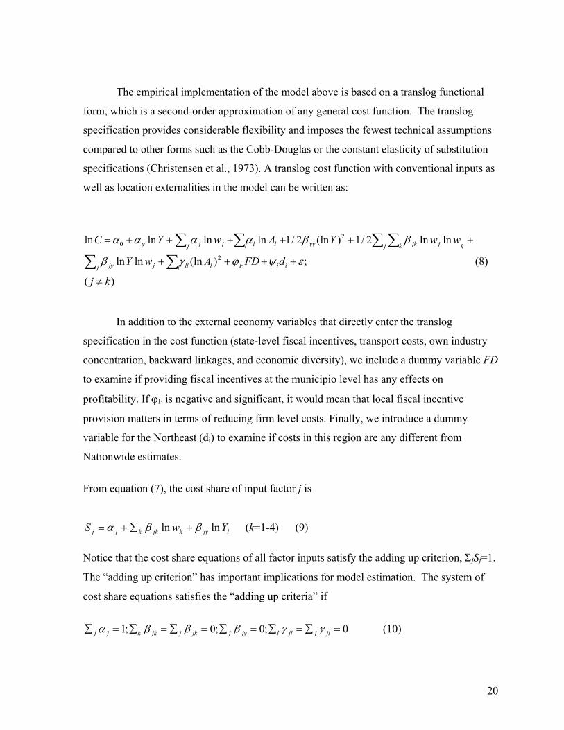
The empirical implementation of the model above is based on a translog functional

form, which is a second-order approximation of any general cost function. The translog

specification provides considerable flexibility and imposes the fewest technical assumptions

compared to other forms such as the Cobb-Douglas or the constant elasticity of substitution

specifications (Christensen et al., 1973). A translog cost function with conventional inputs as

well as location externalities in the model can be written as:

)(

;)(lnlnln

lnln2/1)(ln2/1lnlnlnln2

20

kj

dFDAwY

wwYAwYC

j l iiFllljjy

j kk jjkyyl llj jjy

≠

++++

++++++=

∑ ∑∑ ∑∑∑

εψϕγβ

ββαααα

(8)

In addition to the external economy variables that directly enter the translog

specification in the cost function (state-level fiscal incentives, transport costs, own industry

concentration, backward linkages, and economic diversity), we include a dummy variable FD

to examine if providing fiscal incentives at the municipio level has any effects on

profitability. If ϕF is negative and significant, it would mean that local fiscal incentive

provision matters in terms of reducing firm level costs. Finally, we introduce a dummy

variable for the Northeast (di) to examine if costs in this region are any different from

Nationwide estimates.

From equation (7), the cost share of input factor j is

ljykjkkjj YwS lnln ββα +∑+= (k=1-4) (9) Notice that the cost share equations of all factor inputs satisfy the adding up criterion, ΣjSj=1.

The “adding up criterion” has important implications for model estimation. The system of

cost share equations satisfies the “adding up criteria” if

0;0;0;1 =∑=∑=∑=∑=∑=∑ jljjlljyjjkjjkkjj γγβββα (10)

21

thus reducing the number of free parameters to be estimated.

The translog cost function can be directly estimated from Equation (8); however, a

joint estimation of Equations (8) and (9) with Restriction (10) significantly improves the

efficiency of the model.

The impact of external factors on the cost structure, or profitability, of the firm can be

evaluated by deriving the elasticity of costs with respect to the external economy variables.

From Equation (8) the cost elasticities are:

llllll

AAC ln

lnln γα ∑++=

∂∂ (11)

3.1 Firm Level Data

The translog specification of the production (cost) function requires an exogenous

treatment of factor prices. Unfortunately, we lack exogenous pricing data for the four

production factors included in the model. Therefore, we must rely on the “small player”

assumption that an individual firm is a price taker and cannot significantly influence a

region’s prevailing prices of capital, labor, energy, and materials (KLEM). In general, the

region’s prevailing price is defined as the average price of the factor for sampled firms in the

microregion. The necessary condition of factor price-taking behavior among firms is

preserved insofar individual firms do not contribute significantly to their regional means. To

ensure some homogeneity among the factors to be priced, mean prices are conditional on the

firm’s 4-digit National Classification of Economic Activities (CNAE) code. The prevailing

price of KLEM for each firm is simply the average unit costs of capital, labor, energy, or

materials for firms in the region with common 4-digit industry classifications.

Capital. The prevailing price of capital in each region captures annual leasing rents for

buildings and equipment paid by sampled firms in the microregion. By excluding asset

acquisition, we assume that leasing and purchasing markets are competitive. Therefore, the

22

fraction of the value of accumulated capital stock that factor into production during the

single, surveyed year is equivalent to its leasing price. Although we avoid the potential

arbitrariness of choosing a fixed amortization schedule for heterogeneous assets that

depreciate at differing rates, the validity of our measure of capital rents rests on the

reasonable assumption of competitive purchasing and leasing markets.

We define prevailing regional prices of capital as the average annual lease and rental

payments per dollar of output for a region’s firms in each 4-digit CNAE. Unit capital cost

for each firm in the sample is obtained by dividing annual lease payments by output. The

firm’s price of capital is the mean unit capital cost for firms in the same industry.

Labor. The unit cost of labor is calculated by dividing the total wages and benefits paid by

each firm to its workers employed in its industrial production by the average number of line

workers for the year. The result is the average annual line wage for each firm in the sample.

The average annual line wage should capture the price of labor specific to each 4-digit

CNAE better than total labor costs per worker because the former measure disregards some

possible inefficiencies pertaining to management and other staffing indirectly involved in the

firm’s production. A region’s prevailing wages are defined as mean average annual line

wages for each industry. As there are differences in workers across industries with regard to

skill and productivity, it is reasonable to expect that prevailing wages vary across industries.

Energy. To price energy, we include the firms’ annual costs of fuel and electricity

consumption. Unit energy costs are calculated for each firm by dividing total expenditures

on fuel and electricity by the firm’s total sales of the industrial products (output). The

prevailing energy price for each industry in each microregion is the average of unit energy

costs.

Materials. Data on the stock and flow of materials permit us to calculate the value of

materials consumed during the production year. The value of materials consumed equals the

value of the material stock at the end of the previous year plus purchases during the surveyed

year minus the value of stock at the end of the production year. Unit material costs are the

23

value of the firm’s material consumption divided by its output. Prevailing industry prices for

materials in each region are defined as the average unit material cost for the 4-digit sector.

The KLEM price measures provide reasonable assurance we are modeling factor

price-taking behavior among firms in the PIA sample.

4 RESULTS FROM THE ANALYSIS

The empirical analysis is conducted by jointly estimating equations (8) and (9) as a system

with equation (10) as a restriction. The estimation is conducted using an iterative seemingly

unrelated regression (ITSUR) procedure. The underlying system is nonlinear, and is

primarily derived from the structure of the input demands, as represented in equation (7).

The ITSUR procedure estimates the parameters of the system, accounting for

heteroscedasticity, and contemporaneous correlation in the errors across equations. As the

cost shares sum to unity, n-1 share equations are estimated (where n is the number of

production factors). The ITSUR estimates are asymptotically equivalent to maximum

likelihood estimates and are invariant to the omitted share equation (Greene, 2000). All

estimations were carried out with the MODEL procedure of the SAS system.

As there is considerable variation in the way that firms use technology, make factor

allocation decisions, and can benefit from external economies, we estimate models by firm

size categories in addition to industry wide estimates. For example, smaller firms may be

more reliant on timely and cost efficient access to buyers and suppliers, availability of

ancillary services, inter firm non-technological externalities, and high quality infrastructure.

In contrast, larger firms may be in a better position to internalize production of various

intermediate goods, self-provide infrastructure, and stock higher inventories. Thus, they

would be relatively less dependent on location based amenities and characteristics (Lall et. al.

2003 and 2004). To make allowances for this heterogeneity, and test if in fact there are

differences in production costs and the impact of economic geography and policy instruments

across firms of different sizes, we classify firms into two categories: medium, and large.

24

Medium sized are between 30 and 99 employees and large firms have 100 or more

employees. The number of firms by size category, along with the average number of

employees, unit costs, and output per worker is reported in Table 1. As the PIA data is a

census of all firms with more than 30 employees, the data include all industrial activities in

the sector.

4.1 Fiscal Incentives The first three columns of Table 2 provide the cost elasticities of fiscal incentives, with the

industry-wide elasticities in the first column followed by elasticities for medium and large-

sized firms. The impacts (cost elasticities) of fiscal incentives are estimated using the

specification equation (11). The last three columns of this table provide estimates of ϕF (from

equation 8), which tests if whether or not a municipio offers fiscal incentives matters in terms

of reducing firm level costs. As in the case of the cost elasticities, industry-wide estimates are

followed by estimates for medium and large sized firms.

Let us first consider how federal fiscal incentives offered at the State level influence

firms level costs. The intuition behind using this variable is that if a firm is located in a State

that offers incentives specific to its own industry, then there is a greater likelihood that the

firm will use these incentives to offset production costs. Thus, higher incentives amounts

would translate into lower production costs.

There is considerable variation in the impact of incentives across sectors and firm

sizes. The industry-wide results show that fiscal incentives have a statistically significant cost

reducing effect in four of the twelve study sectors. These are Non Durable manufacturing,

Leather products, Rubber and Plastic, and Metals. For example, the cost elasticity in the

Rubber and Plastic industry is -0.07, which means that doubling the availability of fiscal

incentives will be associated with a 7% decrease in firm level costs. Similarly, the cost

elasticity for Leather products is about -0.144 and for Non Durable Manufacturing is -0.026.

In contrast to these cost reducing effects, we get a rather counter-intuitive results for the

25

Chemicals and Non Metallic Minerals sectors, where providing incentives increases firm

level costs by 6.6% and 2.4% respectively.

Disaggregating the results by firm size, for medium sized firms we find that cost

elasticities are negative and significant in four industry sectors, which are the same sectors as

in the case of the industry-wide estimates. The estimated elasticities are also similar in terms

of magnitude of the effects: -0.032 for Non Durable manufacturing, -0.122 for Leather,

-0.064 for Rubber and Plastic, and -0.032 for Metals. For the Leather industry, this means

that on average, doubling the amount of sector specific fiscal incentives available at the State

level would be associated with a 12.2% reduction in firm level costs for medium sized firms.

In addition to these cost reductions, we also find cost increases associated with State level

incentive provision in the Chemicals (9%) and Non Metallic Minerals industries (2%).

For large size firms, availability of fiscal incentives are associated with cost

reductions in three industry sectors – Printing and Publishing, Rubber and Plastic, and

Metals. For instance, the cost elasticity for Printing and Publishing is 0.065, which means

that a doubling the level of State level fiscal incentives would be associated with a 6.5%

reduction in cost for the average large firm in the sector. In contrast to the medium sized

firms, there are no sectors that show statistically significant cost increases associated with

fiscal incentives.

The last three columns of Table 2 provide parameter estimates for ϕF (equation 8).

From these estimates, it is clear that the indicator variable of ‘whether or not a municipio

offers fiscal incentives’ does not have any significant effect on firm level costs. The only

exception appears to be for the (industry wide) Wood Products sector, where firms in

municipios offering fiscal incentives have about 6.7% lower costs than other similar firms.

We must point out that the indicator variable is rather crude, and does not tell us anything

about the sectoral distribution of incentives.

In general, the results reported in Table 2 show that the impacts of fiscal incentives

are quite modest. For the most part, availability of fiscal incentives do not matter in terms of

26

reducing firm level costs. In particular, sectors requiring considerable capital outlays such as

Mechanical Machinery, Transportation Equipment, and Electrical and Electronics

components do not respond to the availability of these incentives. This could be due to: (a)

the size and composition of the incentive package is not sufficient to offset expenditures to

produce in peripheral or lagging regions, or (b) most firms do not have access to these

incentives even when these are available at the State level (i.e. discretionary incentives are

targeted only to a few firms). More detailed analysis with firm level fiscal incentives data

would be required to identify the exact reasons why fiscal incentives do not have a

significant impact on cost reductions. When fiscal incentives are statistically significant, the

estimated elasticities are quite small, which would suggest that the net benefits from fiscal

incentives would be inadequate to enhance profitability or induce relocation to peripheral

locations.

4.2 Transport Infrastructure

We provide the cost elasticities (calculated from equation 11) for transport costs in

Table 3. The first column provides industry-wide estimates followed by elasticities for

medium and large sized firms. As described earlier in the paper, the transport cost variable

measures the equivalent paved road distance from the microregion to São Paulo. We expect

that firms that have lower equivalent paved road distances9 to São Paulo (the largest market

in the country) would incur lower costs as they can reduce transport costs to supply markets

and satisfy demand. In addition to the pure pecuniary benefits from reducing transport costs,

availability of good infrastructure linking firms to market centers increases the increases the

potential for input diversity, increases probability of technology diffusion through interaction

and knowledge spillovers between firms, as well as between firms and research centers.

Thus, improved accessibility (though lower transport costs) has the effect of reducing

geographic barriers to interaction, which increases specialized labor supply and facilitates

information exchange, technology diffusion and other beneficial spillovers that have a self-

reinforcing effect (see Henderson et. al 2001, Lall et. al 2004; McCann 1998, for a detailed

discussion on this issue).

9 The equivalent road distance measure can be reduced with higher inter regional infrastructure endowments linking the region to São Paulo.

27

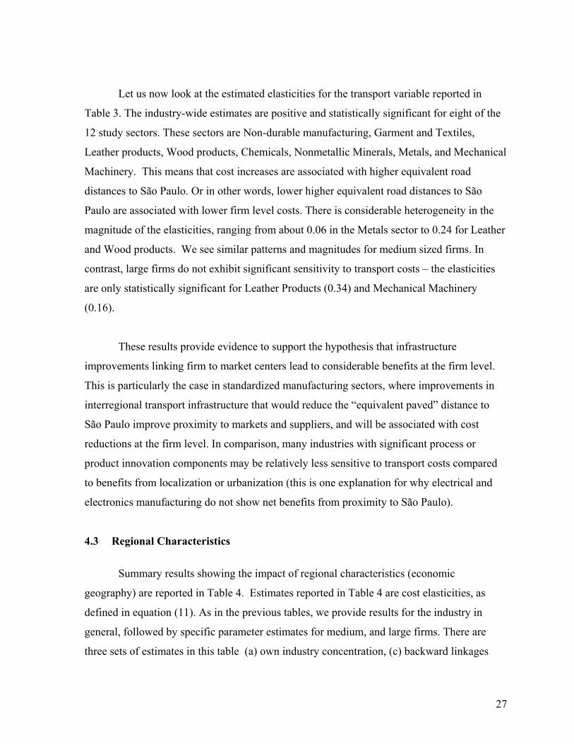
Let us now look at the estimated elasticities for the transport variable reported in

Table 3. The industry-wide estimates are positive and statistically significant for eight of the

12 study sectors. These sectors are Non-durable manufacturing, Garment and Textiles,

Leather products, Wood products, Chemicals, Nonmetallic Minerals, Metals, and Mechanical

Machinery. This means that cost increases are associated with higher equivalent road

distances to São Paulo. Or in other words, lower higher equivalent road distances to São

Paulo are associated with lower firm level costs. There is considerable heterogeneity in the

magnitude of the elasticities, ranging from about 0.06 in the Metals sector to 0.24 for Leather

and Wood products. We see similar patterns and magnitudes for medium sized firms. In

contrast, large firms do not exhibit significant sensitivity to transport costs – the elasticities

are only statistically significant for Leather Products (0.34) and Mechanical Machinery

(0.16).

These results provide evidence to support the hypothesis that infrastructure

improvements linking firm to market centers lead to considerable benefits at the firm level.

This is particularly the case in standardized manufacturing sectors, where improvements in

interregional transport infrastructure that would reduce the “equivalent paved” distance to

São Paulo improve proximity to markets and suppliers, and will be associated with cost

reductions at the firm level. In comparison, many industries with significant process or

product innovation components may be relatively less sensitive to transport costs compared

to benefits from localization or urbanization (this is one explanation for why electrical and

electronics manufacturing do not show net benefits from proximity to São Paulo).

4.3 Regional Characteristics

Summary results showing the impact of regional characteristics (economic

geography) are reported in Table 4. Estimates reported in Table 4 are cost elasticities, as

defined in equation (11). As in the previous tables, we provide results for the industry in

general, followed by specific parameter estimates for medium, and large firms. There are

three sets of estimates in this table (a) own industry concentration, (c) backward linkages

28

and (c) local economic diversity. The results for each industry sector are provided in four

parts. In general, the cost elasticities show that there is considerable heterogeneity in the

impact of location characteristics on firm level costs. This heterogeneity is not limited to the

overall effects across industries, but also includes differences across firms of different sizes

and by sources of agglomeration economies.

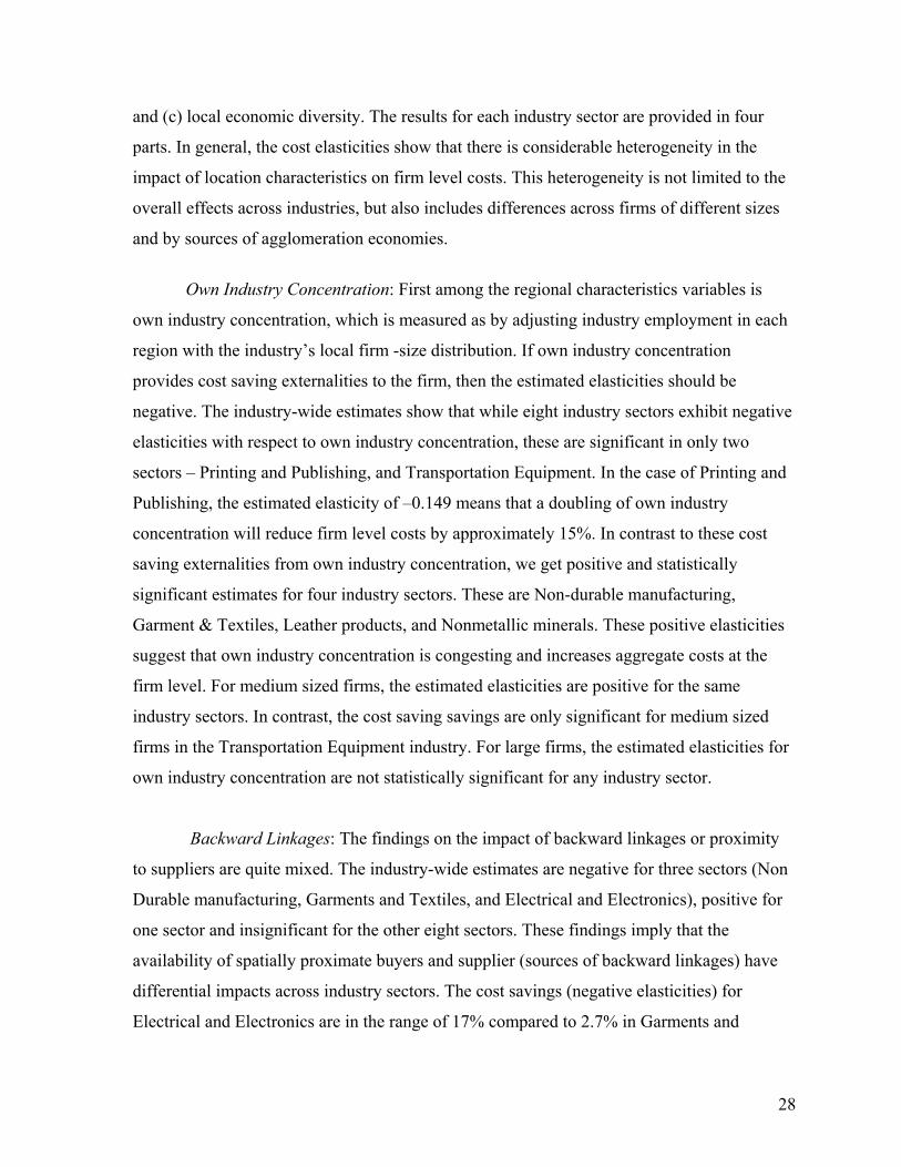
Own Industry Concentration: First among the regional characteristics variables is

own industry concentration, which is measured as by adjusting industry employment in each

region with the industry’s local firm -size distribution. If own industry concentration

provides cost saving externalities to the firm, then the estimated elasticities should be

negative. The industry-wide estimates show that while eight industry sectors exhibit negative

elasticities with respect to own industry concentration, these are significant in only two

sectors – Printing and Publishing, and Transportation Equipment. In the case of Printing and

Publishing, the estimated elasticity of –0.149 means that a doubling of own industry

concentration will reduce firm level costs by approximately 15%. In contrast to these cost

saving externalities from own industry concentration, we get positive and statistically

significant estimates for four industry sectors. These are Non-durable manufacturing,

Garment & Textiles, Leather products, and Nonmetallic minerals. These positive elasticities

suggest that own industry concentration is congesting and increases aggregate costs at the

firm level. For medium sized firms, the estimated elasticities are positive for the same

industry sectors. In contrast, the cost saving savings are only significant for medium sized

firms in the Transportation Equipment industry. For large firms, the estimated elasticities for

own industry concentration are not statistically significant for any industry sector.

Backward Linkages: The findings on the impact of backward linkages or proximity

to suppliers are quite mixed. The industry-wide estimates are negative for three sectors (Non

Durable manufacturing, Garments and Textiles, and Electrical and Electronics), positive for

one sector and insignificant for the other eight sectors. These findings imply that the

availability of spatially proximate buyers and supplier (sources of backward linkages) have

differential impacts across industry sectors. The cost savings (negative elasticities) for

Electrical and Electronics are in the range of 17% compared to 2.7% in Garments and

29

Textiles. On the other hand, there are cost increases (positive elasticites) of 6.1% for Leather

Products, implying that a greater concentration of inter-industry linkages tends to enhance

firm level costs.

When we disaggregate the results by firm size, we find that for medium-sized firms,

net cost savings are observed for Non Durable Manufacturing and Garments and Textiles,

and there are cost increases for the Leather Products industry. Estimated elasticities are not

significant for the other sectors. For large firms, the estimated elasticities are significant for

only one industry sector – Non Durable Manufacturing, where the elasticity of –0.08

signifies cost savings associated with proximity to suppliers.

Economic Diversity: Similar to the estimated elasticities for Backward Linkages,

there are considerable differences in the results for economic diversity across sectors. For the

most part, the Economic Diversity variable has no net impact on firm level costs. When we

look at estimates for all firms, we find a negative and significant elasticity for the

Transportation equipment sector, where the estimate of –13.92 means that costs for a

representative firm in this sector would reduce 14 times with a doubling of diversity. While

this appears to be a very large elasticity, we should keep in mind that any change in the

diversity of the economy involves a large or structural change in the nature and size

distribution of economic activities. The gain to firms in the Transport Equipment sector from

this source of externality primarily stems from the fact that demand for transport related

services increases when there are many sectors in the economy, and that many industries

cluster in areas which have good access to transport networks and services. In comparison,

diversity increases costs for firms in the Garments & Textiles, Nonmetallic Minerals, and

Mechanical Machinery sectors. The increase in net costs due to diversity can partly be

explained by the fact that the costs of higher wages and rents from being located in large and

diverse areas outweigh the benefits of inter-industry linkages and expansion of local demand.

For medium sized firms, the benefits of diversity are observed in the Wood Products

sector. While the elasticity for the Transport Equipment sector is negative, it is not

statistically significant in this case. Net costs from diversity are observed for the same three

30

sectors as in the case of the estimates for all firms. The results for large firms show that there

are considerable gains from diversity in the Printing & Publishing and Transportation

Equipment sectors. The magnitude of the impacts of diversity is bigger for larger firms in

Transport Equipment (-18.4) compared to the industry-wide estimates. In comparison, there

are no statistically significant costs associated with diversity.

In general, we find considerable variation in the impact of regional characteristics

across industry sectors and firm sizes. While there are no clear patterns that emerge from this

part of the analysis, there are a few parameters that are worth exploring in future research.

First, for industries that depend on local demand such as Printing & Publishing and

Transportation Equipment, localization and urbanization economies tend to be cost reducing.

Second, for other standardized industries such as Non-durables, Garments & Textiles ,

Leather, Metals, Non Metallic Minerals and Mechanical Machinery, localization and

urbanization economies are congesting as they tend to push up wages and rents without the

compensating returns from these sources of externalities. Thus, these industries would tend to

locate in smaller or more specialized areas but have access to large markets (see the positive

coefficient on the transport cost variable for these sectors).

5 CONCLUSIONS Many countries have large and sustained differences in sub-national living conditions and

economic performance. Various policy instruments such as infrastructure improvements and

fiscal incentives have been used to alter the national economic landscape and in the process

encourage the growth of lagging sub national regions. However, it is unclear whether in most

instances, these interventions have improved development outcomes of these regions. In this

paper, we examine whether infrastructure improvements and fiscal incentives reduce firm

level costs, thereby influencing firms to locate and produce in areas offering these benefits?

We also examine whether regional characteristics in the form of own industry concentration,

spatially proximate inter-industry linkages, and regional economic diversity reduce costs for

individual firms.

31

In general, we find that lower transport costs or improvement in access to markets are

associated with reductions in firm level costs. This means that firms located in areas with

relatively better market access (measured as the equivalent paved road distance to São Paulo)

tend to have lower costs compared with similar firms in that industry. In comparison, the

effects of fiscal incentives are quite small. In general, provision of state level (sector specific)

fiscal incentives does not reduce firm level costs. This is particularly the case for sectors

requiring considerable capital outlays, such as mechanical machinery, transportation

equipment, and electrical and electronics. Even when the impacts of fiscal incentives are

statistically significant, the estimated elasticities are small enough to suggest that they would

be inadequate to enhance profitability or induce relocation to peripheral locations. There is

considerable inter-industry variation in the impact of regional characteristics. However,

localization and urbanization economies are relatively more important for industries that

depend on local suppliers and demand, such as printing and publishing and transportation

equipment.

What do these results mean for the development of lagging regions? Would the

empirical estimates supporting cost reductions through interregional infrastructure

improvements be the key for developing the lagging Northeast? Most probably not, and for

the following reasons. As most of the study industries produce standardized products,

consumers will purchase products based on price and possibly quality differentials. Further,

existing firms located in agglomerations accrue scale economies from transport savings and

the diversity of input supply. Inter-regional transport improvements that improve the

Northeast’s linkages with the rest of the country will implicitly reduce a natural tariff barrier.

Thus, firms serving larger markets (such as non-basic goods producers in the Southeast) and

benefiting from economies of scale and lower unit costs of production can more easily

expand into new markets in competition with local producers when the unit cost of

distribution between two points is lowered. In the case where manufactured goods are

standardized and product substitution is relatively costless, instead of manufacturing activity

moving to or being created in the Northeast (we may however see a few firms move or start

up)10, we are likely to see that producers in the leading regions (such as São Paulo) will

10 These are likely to be in basic industries serving local demand.

32

expand production and crowd out local producers in the lagging region.11 This may benefit

local consumers in the short run but it will be detrimental for local production and

employment. Thus, it is difficult to say whether transport improvements are likely to have

much development impact on the Northeast.

So what should regional development policy look like? Let us first reiterate that

competition in standardized products is unlikely to be the future for lagging regions,

especially if production of these standardized products is already concentrated or

agglomerated in the leading region, and these products exhibit some degree of increasing

returns to scale. In this context, it may be worth thinking of industry sectors where the

lagging region has comparative advantage – either due to location or (non oil/ mineral) local

/regional endowments, or those that have not yet agglomerated in the leading region. In these

cases, development of upstream and downstream industries along with inter-regional and

local infrastructure improvements may create new markets and growth prospects. More

research on barriers to local development (such as local infrastructure bottlenecks) and new

product innovation opportunities is required to carefully comment on the viability of these

strategies.

11 There are ‘tipping points’ for industry location in agglomerations when congestion costs and wages are high enough to offset net economies from agglomeration. However, these diseconomies are likely to decongest or de-concentrate in the form of spillover developments in areas that are well connected to buyers and suppliers. As figure 2 shows, even though there have been considerable nationwide transport improvements over the past 30-40 years, these have been relatively higher in areas near major market centers, such as Sao Paulo. Thus, connectivity through transport improvements is higher in areas that are also geographically close to the large markets.

33

6 REFERENCES Abdel-Rahman, H. (1988). “Product differentiation, monopolistic competition, and city size.”

Regional Science and Urban Economics, 18, 69-86. Aschauer, D. A. (1989). “Is public expenditure productive?” Journal of Monetary Economics, 23,

177-200. Azzoni, C. R., N. Menezes-Filho, T. A. de Menezes and R. Silveira-Neto (2002). “Geography and

Income Convergence Among Brazilian States.” Mimeo. Baer, W. (1995). The Brazilian Economy: Growth and Development. 4th ed. Westport: Praeger. Bartik, T. J. (1985). “Business Location Decisions in the United States: Estimates of the Effects of

Unionization, taxes, and Other Characteristics of States.” Journal of Business and Economic Statistics, 3, 1, 14-22.

Biehl, D. (1986). “The Contribution of Infrastructure to Regional Development.” Regional Policy Division, European Communities, Brussels.

Bostic, R. (1997). “Urban productivity and factor growth in the late 19th century.” Journal of Urban Economics, 4, 38-55.

Castro, N. (2002). "Transportation costs and Brazilian agricultural production: 1970-1996" Texto para Discussão - NEMESIS – LXVI, http://ssrn.com/author=243495", Social Science Research Network.

Castro , N. (2003). “Logistic Costs and Brazilian Regional Development.” Mimeo. Chinitz, B. (1961). “Contrasts in agglomeration: New York and Pittsburgh.” American Economic

Review, 51, 279-289. Christensen, L., D. Jorgenson, and L. Lau. (1973). “Transcendental logarithmic production function

frontiers.” Review of Economics and Statistics 55, 29–45. Ciccone, A., and R. Hall. (1996). “Productivity and the density of economic activity.” American

Economic Review, 86, 54-70. Ferreira, P. C. (2003). “Regional Policy in Brazil: a Review.” Mimeo Ferreira, A.H.B. (2000). “Convergence in Brazil: Recent Trends and Long Run Prospects.” Applied

Economics, 32, 479-489. Feser, E. J. (2002). “Tracing the sources of local external economies.” Urban Studies, 39, 13, 2485-

2506. Feser, E. J., and E.M. Bergman. (2000). “National industry cluster templates: a framework for applied

regional cluster analysis.” Regional Studies, 34, 1-20. Fujita, M., (1989). Urban economic theory. Land Use and City Size. Cambridge Univ. Press,

Cambridge, MA. Fujita, M., P. Krugman, and A. Venables (1999). The Spatial Economy: Cities, Regions, and

International Trade. Cambridge, MA: MIT Press. Garcia-Mila, T., and T. McGuire (1993). “Industrial mix as a factor in the growth and variability of

state's economies.” Regional Science and Urban Economics, 23, 731-748. Goldsmith, W. and R. Wilson. 1991. “Poverty and Distorted Industrialization in the Northeast.”

World Development, 19,5, 435-55. Greene, W. (2000). Econometric Analysis. Upper Saddle River, NJ: Prentice-Hall. Heckman, J. J. (1979). “Sample Selection Bias as a Specification Error.” Econometrica, 47, 153-61. Henderson, J. V. (1988). Urban Development: Theory, Fact, and Illusion. New York: Oxford Univ.

Press. Henderson, J.V., T. Lee, and Y.J. Lee (2001). “Scale Externalities in Korea.” Journal of Urban

Economics, 49, 479-504. Henderson, J. V., Z. Shalizi, and A. Venables (2001). “Geography and development.” Journal of

Economic Geography 1 (1), 81– 105. Hirschman, A. (1958). The Strategy of Economic Development. New Haven: Yale University Press.

34

Jacobs, J. (1969). The Economy of Cities. New York: Vintage. Kieschnick (1981). “Taxes and Growth - Business Incentives and Economic Development.” Studies

in Development Policy, Council of State Planning Agencies, Washington DC. Krugman, P. (1991a). Geography and Trade. Cambridge, Mass.: MIT Press. Krugman, P. (1991b). “Increasing returns and economic geography.” Journal of Political Economy,

99, 483-499. Lall, S. V. (1996) “A Review of Economic Analysis for World Bank Infrastructure Projects.”

Prepared for the Policy Research Department, World Bank, Washington DC. Lall S. V., J. Koo and S. Chakravorty (2003) “Diversity Matters: The Economic Geography of

Industry Location in India.” World Bank Policy Research Working Paper 3072, Washington, DC.

Lall, S.V., Z. Shalizi and U. Deichmann, U. (2004) “Agglomeration economies and productivity in Indian industry.” Journal of Development Economics. In press

Lall, S. V. and Z. Shalizi (2003) “Location and growth in the Brazilian Northeast.” Journal of Regional Science, 43, 4, 1-19.

Markusen, A. (1994). “Interaction Between Regional and Industrial Policies: Evidence from Four Countries.” Proceedings of the World Bank Annual Conference on Development Economics, Washington, D.C.

Marshall, A. (1890). Principles of Economics. London: Macmillan. Marshall, A. (1919). Industry and Trade. London: Macmillan. McCann, P. (1998). The economics of industrial location: a logistics-costs approach. Series on

Advances in Spatial Science. Springer, Heidelberg. Nadiri, M.I. (1970). “International Studies of Factor Inputs and Total Factor Productivity: A Brief

Survey.” Review of Income and Wealth, 18, 129-48. Nurske, R. (1953). Problems of Capital Formation in Underdeveloped Countries. Basil Blackwell. Parr, J. B. (1999). “Growth-pole Strategies in Regional Economic Planning: A Retrospective View.

Part 1. Origins and Advocacy.” Urban Studies, 36, 7, 1195 – 1215. Rivera-Batiz, F. (1988). “Increasing returns, monopolistic competition, and agglomeration economies

in consumption and production.” Regional Science and Urban Economics, 18, 125-154. Rosenstein-Rodan, P. (1943). “The Problem of Industrialization of Eastern and South-Eastern

Europe.” Economic Journal, 53, 202-211. Venables, A. (1996). “Equilibrium locations of vertically linked industries.” International Economic

Review, 49, 341-359. World Bank. (1987). Brazil: Industrial Development Issues of the Northeast. World Bank Economic

and Sector Report. Washington, D.C. World Bank. (1998). Public Expenditures for Poverty Alleviation in Northeast Brazil: Promoting

Growth and Improving Services. World Bank Report 18700-BR. December. Yepes, T., S.V. Lall, and D. Salvi. 2004. “Tax Incentives in Brazilian Industry.” Mimeo. World Bank

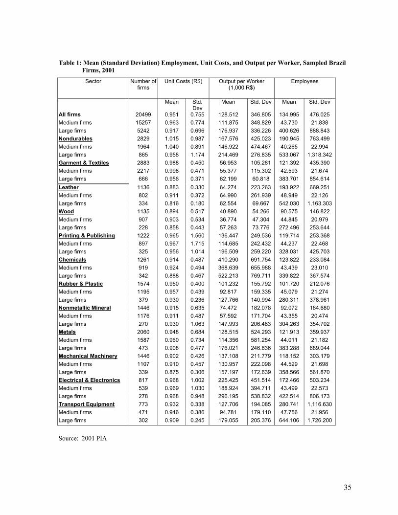
35

Table 1: Mean (Standard Deviation) Employment, Unit Costs, and Output per Worker, Sampled Brazil

Firms, 2001 Sector Number of

firms Unit Costs (R$)

Output per Worker

(1,000 R$)

Employees

Mean Std. Dev

Mean Std. Dev Mean Std. Dev

All firms 20499 0.951 0.755 128.512 346.805 134.995 476.025 Medium firms 15257 0.963 0.774 111.875 348.829 43.730 21.838 Large firms 5242 0.917 0.696 176.937 336.226 400.626 888.843 Nondurables 2829 1.015 0.987 167.576 425.023 190.945 763.499 Medium firms 1964 1.040 0.891 146.922 474.467 40.265 22.994 Large firms 865 0.958 1.174 214.469 276.835 533.067 1,318.342 Garment & Textiles 2883 0.988 0.450 56.953 105.281 121.392 435.390 Medium firms 2217 0.998 0.471 55.377 115.302 42.593 21.674 Large firms 666 0.956 0.371 62.199 60.818 383.701 854.614 Leather 1136 0.883 0.330 64.274 223.263 193.922 669.251 Medium firms 802 0.911 0.372 64.990 261.939 48.949 22.126 Large firms 334 0.816 0.180 62.554 69.667 542.030 1,163.303 Wood 1135 0.894 0.517 40.890 54.266 90.575 146.822 Medium firms 907 0.903 0.534 36.774 47.304 44.845 20.979 Large firms 228 0.858 0.443 57.263 73.776 272.496 253.644 Printing & Publishing 1222 0.965 1.560 136.447 249.536 119.714 253.368 Medium firms 897 0.967 1.715 114.685 242.432 44.237 22.468 Large firms 325 0.956 1.014 196.509 259.220 328.031 425.703 Chemicals 1261 0.914 0.487 410.290 691.754 123.822 233.084 Medium firms 919 0.924 0.494 368.639 655.988 43.439 23.010 Large firms 342 0.888 0.467 522.213 769.711 339.822 367.574 Rubber & Plastic 1574 0.950 0.400 101.232 155.792 101.720 212.076 Medium firms 1195 0.957 0.439 92.817 159.335 45.079 21.274 Large firms 379 0.930 0.236 127.766 140.994 280.311 378.961 Nonmetallic Mineral 1446 0.915 0.635 74.472 182.078 92.072 184.680 Medium firms 1176 0.911 0.487 57.592 171.704 43.355 20.474 Large firms 270 0.930 1.063 147.993 206.483 304.263 354.702 Metals 2060 0.948 0.684 128.515 524.293 121.913 359.937 Medium firms 1587 0.960 0.734 114.356 581.254 44.011 21.182 Large firms 473 0.908 0.477 176.021 246.836 383.288 689.044 Mechanical Machinery 1446 0.902 0.426 137.108 211.779 118.152 303.179 Medium firms 1107 0.910 0.457 130.957 222.098 44.529 21.698 Large firms 339 0.875 0.306 157.197 172.639 358.566 561.870 Electrical & Electronics 817 0.968 1.002 225.425 451.514 172.466 503.234 Medium firms 539 0.969 1.030 188.924 394.711 43.499 22.573 Large firms 278 0.968 0.948 296.195 538.832 422.514 806.173 Transport Equipment 773 0.932 0.338 127.706 194.085 280.741 1,116.630 Medium firms 471 0.946 0.386 94.781 179.110 47.756 21.956 Large firms 302 0.909 0.245 179.055 205.376 644.106 1,726.200

Source: 2001 PIA

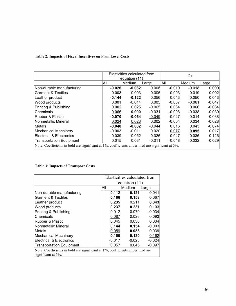
36

Table 2: Impacts of Fiscal Incentives on Firm Level Costs

Elasticities calculated from equation (11)

ϕF

All Medium Large All Medium Large Non-durable manufacturing -0.026 -0.032 0.006 -0.019 -0.018 0.009Garment & Textiles 0.003 0.003 0.006 0.003 0.019 0.002Leather product -0.144 -0.122 -0.056 0.043 0.050 0.043Wood products 0.001 -0.014 0.005 -0.067 -0.061 -0.047Printing & Publishing 0.002 0.025 -0.065 0.064 0.066 -0.034Chemicals 0.066 0.090 -0.031 -0.006 -0.038 -0.039Rubber & Plastic -0.070 -0.064 -0.049 -0.027 -0.014 -0.038Nonmetallic Mineral 0.024 0.023 0.002 -0.004 0.034 -0.028Metals -0.040 -0.032 -0.044 0.016 0.043 -0.074Mechanical Machinery -0.003 -0.011 0.020 0.077 0.095 0.017Electrical & Electronics 0.039 0.052 0.026 -0.047 -0.036 -0.126Transportation Equipment 0.015 0.031 -0.011 -0.048 -0.032 -0.029Note: Coefficients in bold are significant at 1%, coefficients underlined are significant at 5%.

Table 3: Impacts of Transport Costs

Elasticities calculated from equation (11)

All Medium Large Non-durable manufacturing 0.112 0.121 0.041Garment & Textiles 0.166 0.158 0.067Leather product 0.235 0.211 0.343Wood products 0.237 0.231 0.103Printing & Publishing 0.012 0.070 -0.034Chemicals 0.087 0.026 0.093Rubber & Plastic 0.045 0.036 0.034Nonmetallic Mineral 0.144 0.154 -0.003Metals 0.059 0.083 0.039Mechanical Machinery 0.150 0.120 0.162Electrical & Electronics -0.017 -0.023 -0.024Transportation Equipment 0.057 0.045 -0.097Note: Coefficients in bold are significant at 1%, coefficients underlined are significant at 5%.

37

Table 4: Impacts of Regional Characteristics

Own Industry Employment -

Localization Backward Linkages - IO Manufacturing Diversity All Medium Large All Medium Large All Medium Large Non-durable manufacturing 0.095 0.076 0.095 -0.071 -0.044 -0.080 0.088 0.095 -0.054Garment & Textiles 0.111 0.110 -0.060 -0.027 -0.024 0.002 0.726 0.949 0.753Leather product 0.086 0.094 -0.015 0.061 0.064 0.026 -0.330 -0.649 -0.101Wood products -0.004 -0.010 -0.040 -0.010 0.010 0.040 -0.064 -2.758 0.051Printing & Publishing -0.149 -0.135 0.085 0.041 0.068 -0.102 -0.437 2.563 -3.406Chemicals -0.020 -0.010 -0.116 -0.004 -0.042 -0.031 -2.875 -3.413 -8.711Rubber & Plastic -0.045 -0.031 -0.059 -0.034 -0.032 -0.029 2.322 2.786 1.517Nonmetallic Mineral 0.121 0.147 -0.028 -0.021 -0.029 0.129 1.026 0.923 0.791Metals -0.032 -0.032 -0.002 0.013 0.044 0.011 2.357 1.234 2.130Mechanical Machinery -0.019 -0.024 0.012 0.039 0.016 0.072 8.767 6.496 20.434Electrical & Electronics -0.061 -0.090 -0.034 -0.171 -0.184 -0.275 6.569 7.519 -1.532Transportation Equipment -0.102 -0.120 -0.066 -0.064 -0.058 -0.140 -13.942 -7.125 -18.410Note: Coefficients in bold are significant at 1%, coefficients underlined are significant at 5%.

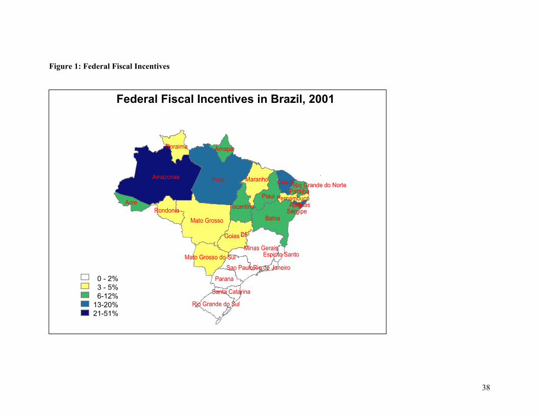
38

Figure 1: Federal Fiscal Incentives

Federal Fiscal Incentives in Brazil, 2001

0 - 2%3 - 5%6-12%

13-20%21-51%

ParaAmazonas

BahiaMato Grosso

Goias

Piaui

Minas Gerais

Maranho

Acre

Parana

Tocantins

Roraima

Sao Paulo

Rondonia

Ceara

Amapa

Mato Grosso do Sul

Rio Grande do Sul

PernambucoParaiba

Santa Catarina

Espirito Santo

Alagoas

Rio de Janeiro

Sergipe

Rio Grande do Norte

DF

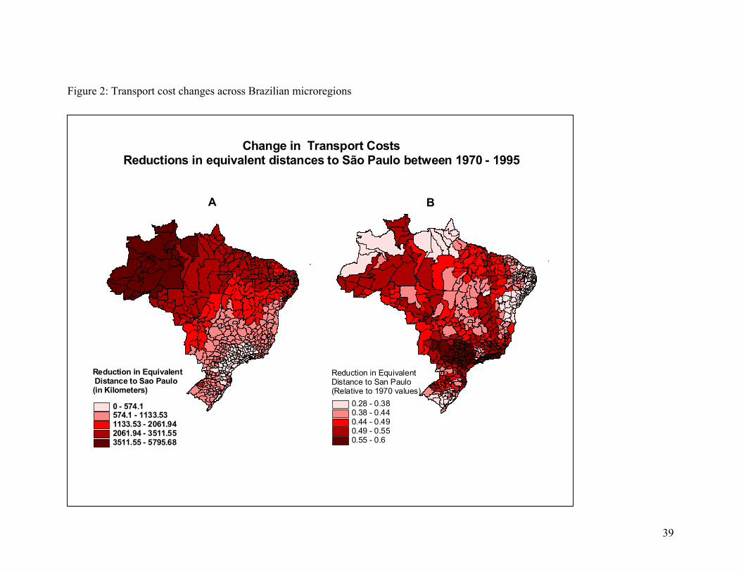
39

Figure 2: Transport cost changes across Brazilian microregions

Change in Transport CostsReductions in equivalent distances to São Paulo between 1970 - 1995

Reduction in Equivalent Distance to Sao Paulo (in Kilometers)

0 - 574.1574.1 - 1133.531133.53 - 2061.942061.94 - 3511.553511.55 - 5795.68

Reduction in Equivalent Distance to San Paulo(Relative to 1970 values)

0.28 - 0.380.38 - 0.440.44 - 0.490.49 - 0.550.55 - 0.6

A B

40

Figure 3: Spatial Distribution of Economic Activity in Brazil

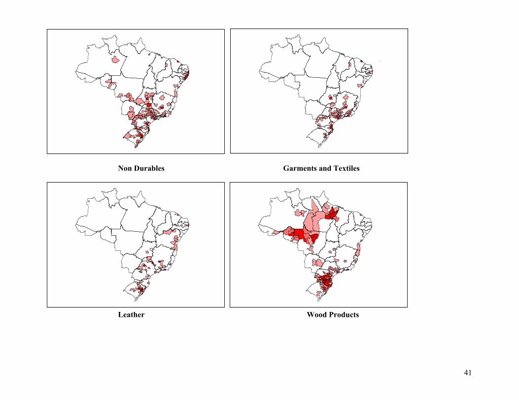
41

Non Durables Garments and Textiles

Leather Wood Products

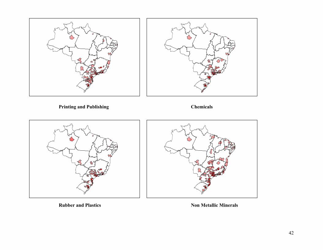
42

Printing and Publishing Chemicals

Rubber and Plastics Non Metallic Minerals

43

Metals Mechanical Machinery

Electrical and Electronics Transport Equipment