location awareness in cognitive radio networks
TRANSCRIPT

University of South FloridaScholar Commons
Graduate Theses and Dissertations Graduate School
6-24-2008
Location Awareness in Cognitive Radio NetworksHasari CelebiUniversity of South Florida
Follow this and additional works at: https://scholarcommons.usf.edu/etd
Part of the American Studies Commons
This Dissertation is brought to you for free and open access by the Graduate School at Scholar Commons. It has been accepted for inclusion inGraduate Theses and Dissertations by an authorized administrator of Scholar Commons. For more information, please [email protected].
Scholar Commons CitationCelebi, Hasari, "Location Awareness in Cognitive Radio Networks" (2008). Graduate Theses and Dissertations.https://scholarcommons.usf.edu/etd/167

Location Awareness in Cognitive Radio Networks
by
Hasari Celebi
A dissertation submitted in partial fulfillmentof the requirements for the degree of
Doctor of PhilosophyDepartment of Electrical Engineering
College of EngineeringUniversity of South Florida
Major Professor: Huseyin Arslan, Ph.D.Frederick Martin , Ph.D.
Miguel A. Labrador, Ph.D.Thomas Weller, Ph.D.Leslaw Skrzypek, Ph.D.Paris H. Wiley, Ph.D.
Date of Approval:June 24, 2008
Keywords: cognitive positioning systems, dynamic spectrum access, dispersed spectrum utilization,environment awareness, location sensing, Cramer-Rao lower bound, range accuracy adaptation,
time delay estimation, whole spectrum utilization
c© Copyright 2008, Hasari Celebi

DEDICATION
To my family and parents.

ACKNOWLEDGEMENTS
I wish to express my gratitude to my advisor, Dr. Huseyin Arslan, for his guidance and continu-
ous encouragement throughout the development of this dissertation. It has been very enjoyable and
fruitful to work under his supervision and learn from him. His helpful discussions and comments
initiates many new ideas and research directions with successful results presented in this dissertation.
I wish to thank each committee member: Dr. Frederick Martin, Dr. Miguel A. Labrador, Dr.
Thomas Weller, Dr. Leslaw Skrzypek, and Dr. Paris H. Wiley for serving in my committee, their
valuable times, feedbacks, and recommendations that improve the quality of this dissertation. In
addition, I appreciate Dr. Carlos Smith for chairing my dissertation defense session. Furthermore,
many thanks to the administration and staff of the Electrical Engineering department, especially
Gayla Montgomery, Irene Wiley, Maria Du, Becky Brenner, and Norma Paz for their kind helps
throughout my doctoral study.
Special thanks go to Dr. Sinan Gezici for his help and comments on the development of some
parts in Chapter 5 of this dissertation. In addition, Mohammad Juma deserves acknowledgement for
providing some measurement results in Chapter 7 of this dissertation. The administration of Logus
Broadband Wireless Solutions Inc. and Honeywell definitely deserves many thanks for supporting
myself financially during my doctoral study.
I wish to thank my friends in wireless communications and signal processing group: Dr. Kemal
Ozdemir, Dr. Ismail Guvenc, Dr. Tevfik Yucek, Serhan Yarkan, Mustafa E. Sahin, Hisham A.
Mahmoud, Sadia Ahmed, Ali Gorcin, Sabih Guzelgoz, Ahmed Hesham, Evren Terzi, and Omar H.
Zakaria. I enjoyed working and sharing many things with them. I wish the best for all of them in
their future careers and lives.
I would like to express my deepest gratitude to my wife for her encouragement and patience
throughout my doctoral study. You always were there to share my concerns and happiness and
whenever I need hope and motivation. Especially, you took care of our lovely two sons, Yusuf and
Enes, in my absence at home and allowing me study long hours at the school. I will never forget your
support, patience, understanding, and sacrifice. Finally, I would like to thank to my dear parents,
brothers, and sister for their continuous supports, sacrifices, and encouragements over the years.

TABLE OF CONTENTS
LIST OF TABLES iv
LIST OF FIGURES v
ABSTRACT viii
CHAPTER 1 INTRODUCTION 11.1 Location and Environment Awareness in the Nature 21.2 Location and Environment Awareness in Wireless Systems 31.3 Cognitive Radio with Location and Environment Awareness Capabilities 51.4 Overview of the Dissertation 7
1.4.1 Chapter 2: Location and Environment Awareness in Cog-nitive Radios 7
1.4.2 Chapter 3: Cognitive Positioning Systems 71.4.3 Chapter 4: Time Delay Estimation Using Whole Spectrum
Utilization Approach 81.4.4 Chapter 5: Time Delay Estimation Using Dispersed Spec-
trum Utilization Approach 81.4.5 Chapter 6: Comparison of Whole and Dispersed Spectrum
Utilization for Time Delay Estimation 91.4.6 Chapter 7: Location Aware Systems in Cognitive Wireless Networks 9
CHAPTER 2 LOCATION AND ENVIRONMENT AWARENESS INCOGNITIVE RADIOS 10
2.1 Introduction 102.2 Proposed Cognitive Radio Architecture 11
2.2.1 Sensing Interface 132.2.1.1 Radiosensing Sensors 132.2.1.2 Radiovision Sensors 142.2.1.3 Radiohearing Sensors 14
2.2.2 Location Awareness Engine 162.2.2.1 Location Sensing Methods 162.2.2.2 Seamless Positioning and Interoperability 212.2.2.3 Security and Privacy 222.2.2.4 Statistical Learning and Tracking 232.2.2.5 Mobility Management 232.2.2.6 Adaptation of Location Aware Systems 23
2.2.3 Environment Awareness Engine 242.2.3.1 Topographical Information 262.2.3.2 Object Recognition and Tracking 262.2.3.3 Propagation Characteristics 262.2.3.4 Meteorological Information 27
2.3 Conclusions 28
i

CHAPTER 3 COGNITIVE POSITIONING SYSTEMS 293.1 Introduction 293.2 Range Accuracy Adaptation 31
3.2.1 Transmitter for Range Accuracy Adaptation 323.2.2 Receiver for Range Accuracy Adaptation 353.2.3 Proposed ML Range Accuracy Adaptation 353.2.4 Main Error Sources 36
3.2.4.1 Dynamic Spectrum Effects 373.2.4.2 Transceiver Effects 383.2.4.3 Environmental Effects 383.2.4.4 Interference Effects 39
3.2.5 Simulation Results for ML Range Accuracy Adaptation 393.3 Performance Improvement Approaches for Range Accuracy Adaptation 41
3.3.1 Dynamic Spectrum Access Systems 423.3.1.1 Overlay Dynamic Spectrum Access Technique 443.3.1.2 Hybrid Overlay and Underlay Dynamic Spectrum
Access Technique 443.3.1.3 Discussions 47
3.4 Conclusions 49
CHAPTER 4 TIME DELAY ESTIMATION USING WHOLE SPECTRUM UTILIZATIONAPPROACH 51
4.1 Ranging in Dynamic Spectrum Access Systems 514.1.1 System Model 524.1.2 The Asymptotic Frequency-domain Cramer-Rao Bound 53
4.2 Ranging Related Channel Statistics 544.2.1 IEEE 802.15.4a Channel Models 564.2.2 The Effects of Receiver Architectures 574.2.3 Channel Statistics for Practical TOA Ranging Algorithms 58
4.2.3.1 Statistics of Amplitude and Phase of the LeadingEdge and Peak Samples 58
4.2.3.2 Statistics of the Delay Between the Leading Edgeand Peak Samples 58
4.2.3.3 Statistics of Number of Clusters Prior to the Peak Sample 594.2.3.4 Statistics of Number of Delays Between Clusters
that are Prior to the Peak Sample 594.2.4 Results and Discussions 59
4.3 Conclusions 66
CHAPTER 5 TIME DELAY ESTIMATION USING DISPERSED SPECTRUM UTILIZA-TION APPROACH 67
5.1 Introduction 675.2 Signal Model 685.3 CRLB Calculations 695.4 Special Cases 725.5 Numerical Results 755.6 Concluding Remarks 77
ii

CHAPTER 6 COMPARISON OF WHOLE AND DISPERSED SPECTRUM UTILIZATIONFOR TIME DELAY ESTIMATION 79
6.1 Introduction 796.2 System and Signal Model 80
6.2.1 Cognitive Radio Transceiver for Whole Spectrum Utilization 816.2.2 Cognitive Radio Transceiver for Dispersed Spectrum Utilization 82
6.3 CRLB for Whole and Dispersed Spectrum Utilization Systems 836.4 A Combining Technique for Dispersed Spectrum Utilization Systems 866.5 Results and Discussions 866.6 Conclusions 89
CHAPTER 7 LOCATION AWARE SYSTEMS IN COGNITIVE WIRELESS NETWORKS 927.1 Introduction 927.2 Cognitive Wireless Network Model 937.3 Implementation Options 947.4 Location-based Services 987.5 Location-assisted Network Optimization 98
7.5.1 Location-assisted Dynamic Spectrum Management 987.5.2 Location-assisted Network Plan and Expansion 1017.5.3 Location-assisted Handover 103
7.6 Conclusions 106
CHAPTER 8 CONCLUSIONS AND FUTURE WORKS 107
REFERENCES 112
APPENDICES 119Appendix A FIM Elements 120Appendix B Derivation of CRLB for Dispersed Spectrum Utilization 121
ABOUT THE AUTHOR End Page
iii

LIST OF TABLES
Table 3.1 A numerical example for determining d and dth. 46
Table 4.1 The measured κ values of some UWB channels. 60
Table 4.2 The τple values in ns for different channel models that have a proba-bility of 5 · 10−4. 62
Table 4.3 The values of Ep and Ele for different channel models. 62
Table 7.1 Some representative location aware applications for cognitive radiosand networks. 99
Table 7.2 An illustrative snapshot of local geolocation-database. 101
Table 7.3 An example of geographic table that is formed by location-assistednetwork plan and expansion method. 102
iv
LIST OF FIGURES
Figure 1.1 Illustration of location and environment awareness in bat echolocation system. 3
Figure 1.2 Illustration of location and environment awareness in human beingusing eyes and ears (Human head image by courtesy of [1]). 3
Figure 1.3 Simplified conceptual model of location and environment awarenesscycles for the creatures (e.g. human, bat). 4
Figure 1.4 Simplified block diagram for a cognitive radio system. 6
Figure 2.1 A conceptual model for cognitive radio systems with location andenvironment awareness cycles and engines. 12
Figure 2.2 Block diagram of location awareness engine for cognitive radios and networks. 16
Figure 2.3 A taxonomy of location information. 18
Figure 2.4 A conceptual model for environment awareness engine. 25
Figure 3.1 Block diagram of cognitive radio transceiver for range accuracy adaptation. 36
Figure 3.2 Performance of maximum likelihood range accuracy adaptation inwhole spectrum utilization case. 42
Figure 3.3 Bandwidth adaptation in maximum likelihood range accuracy adaptation. 43
Figure 3.4 The effects of maximum dynamic range (κmax) on the distance thresh-old (dth). 48
Figure 4.1 Illustration of time of arrival (TOA) ranging related channel statistics. 58
Figure 4.2 The effects of absolute bandwidth (top figure) and center frequency(bottom figure) on the standard deviation of the distance estimationerror in log scale. 60
Figure 4.3 The effects of frequency dependency of the channel environment onthe standard deviation of the distance estimation error in log scale. 61
Figure 4.4 The statistics of the delay between the peak and leading edge sample(τple) based on channel impulse response for line of sight (LOS) andnon-line of sight (NLOS) environments. 63
v

Figure 4.5 The statistics of the delay between the peak and leading edge sample(τple) based on energy block for line of sight (LOS) and non-line ofsight (NLOS) environments. 64
Figure 4.6 Number of clusters prior to the peak sample (Λ) and number of delaysbetween clusters that are prior to the peak sample (γ) statistics forline of sight (LOS) environments. 65
Figure 4.7 Number of clusters prior to the peak sample (Λ) and number of delaysbetween clusters that are prior to the peak sample (γ) statistics fornon-line of sight (NLOS) environments. 65
Figure 5.1 Illustration of dispersed spectrum utilization in cognitive radio systems. 69
Figure 5.2 Block diagram of a cognitive radio receiver. 70
Figure 5.3√
CRLB versus SNR for K = 3 and N = 2. 76
Figure 5.4√
CRLB versus SNR for K = 3 and N = 16. 77
Figure 5.5√
CRLB versus K for N = 16 and 16PSK modulation when the SNRis defined as the sum of the SNRs at different branches. 78
Figure 5.6√
CRLB versus K for N = 16 and 16PSK modulation when the SNRis defined per branch. 78
Figure 6.1 Illustration of whole spectrum utilization in cognitive radio systems. 80
Figure 6.2 Illustration of dispersed spectrum utilization in cognitive radio systems. 80
Figure 6.3 Block diagram of cognitive radio transceiver for whole and dispersedspectrum utilization. 81
Figure 6.4 Block diagram of cognitive radio transceiver for the whole spectrum utilization. 82
Figure 6.5 Block diagram of cognitive radio transceiver for the dispersed spec-trum utilization. 83
Figure 6.6 Energy combining technique for dispersed spectrum utilization systems. 86
Figure 6.7 Comparison of exact and approximate CRLB for whole spectrum uti-lization systems. 88
Figure 6.8 RMSE of ML TOA estimator and√
CRLB versus SNR for dispersedand whole spectrum utilization techniques considering simulation pa-rameters in case 1. 90
Figure 6.9 RMSE of ML TOA estimator and√
CRLB versus SNR for dispersedand whole spectrum utilization techniques considering simulation pa-rameters in case 2. 91
Figure 6.10 RMSE of ML TOA estimator and√
CRLB versus SNR for dispersedand whole spectrum utilization techniques considering simulation pa-rameters in case 3. 91
vi

Figure 7.1 Illustration of the homogeneous pure cognitive wireless networks; textin the parentheses show the instantaneous waveform of each cognitiveradio node (CR: cognitive radio node). 95
Figure 7.2 Illustration of the mixed cognitive and non-cognitive wireless networks(NCR: non-cognitive radio nodes). 96
Figure 7.3 A conceptual model for cooperative location awareness between twocognitive radios. 96
Figure 7.4 Illustration of cognitive ranging protocol. 97
Figure 7.5 A conceptual model for self location awareness: a) active, b) passive. 97
Figure 7.6 Test phone (MS2) in the dedicated mode: a) signal quality, b) signalstrength, c) handover pattern. 104
Figure 7.7 Test phone (MS1) in the locked mode: a) signal quality, b) signal strength. 105
vii
LOCATION AWARENESS IN COGNITIVE RADIO NETWORKS
Hasari Celebi
ABSTRACT
Cognitive radio is a recent novel approach for the realization of intelligent and sophisticated
wireless systems. Although the research and development on cognitive radio is still in the stage of
infancy, there are significant interests and efforts towards realization of cognitive radio. Cognitive
radio systems are envisioned to support context awareness and related systems. The context can be
spectrum, environment, location, waveform, power and other radio resources. Significant amount
of the studies related to cognitive radio in the literature focuses on the spectrum awareness since it
is one of the most crucial features of cognitive radio systems. However, the rest of the features of
cognitive radio such as location and environment awareness have not been investigated thoroughly.
For instance, location aware systems are widespread and the demand for more advanced ones are
growing. Therefore, the main objective of this dissertation is to develop an underlying location
awareness architecture for cognitive radio systems, which is described as location awareness engine,
in order to support goal driven and autonomous location aware systems.
A cognitive radio conceptual model with location awareness engine and cycle is developed by
inspiring from the location awareness features of human being and bat echolocation systems. Addi-
tionally, the functionalities of the engine are identified and presented. Upon providing the function-
alities of location awareness engine, the focus is given to the development of cognitive positioning
systems. Furthermore, range accuracy adaptation, which is a cognitive behavior of bats, is developed
for cognitive positioning systems.
In what follows, two main approaches are investigated in order to improve the performance of
range accuracy adaptation method. The first approach is based on idea of improving the spec-
trum availability through hybrid underlay and overlay dynamic spectrum access method. On the
other hand, the second approach emphasizes on spectrum utilization, where we study performance
viii

of range accuracy adaptation from both theoretical and practical perspectives considering whole
spectrum utilization approach. Furthermore, we introduced a new spectrum utilization technique
that is referred as dispersed spectrum utilization. The performance analysis of dispersed spectrum
utilization approach is studied considering time delay estimation problem in cognitive positioning
systems. Afterward, the performance of whole and dispersed spectrum utilization approaches are
compared in the context of cognitive positioning systems.
Finally, some representative advanced location aware systems for cognitive radio networks are
presented in order to demonstrate some potential applications of the proposed location awareness
engine in cognitive radio systems.
ix

CHAPTER 1
INTRODUCTION
Cognitive radio is a promising concept for the realization of smart and advanced wireless systems.
One of the main features of cognitive radio is to support context awareness such as spectrum, loca-
tion, environment, waveform, power, and infrastructure awareness. The majority of cognitive radio
studies in the literature are focused on spectrum awareness capability of cognitive radio systems.
The remainder features of cognitive radio systems such as location awareness has not been studied
thoroughly.
Location awareness term in this dissertation is defined to embody sensing, learning, decision
making, and adaptation of location information. Location information has been traditionally used for
positioning systems and consequently location-based services (LBS). Nevertheless, the demands on
higher quality of services (QoS) such as goal driven and autonomous location aware applications from
mobile users as well as wireless network operators motivate system designers to exploit utilization of
location information in wireless networks. Recently, it has been realized that LBS are not the only
applications where location information can be used. It can be utilized for different applications
and solving some issues in wireless networks. The applications based on utilization of location
information (i.e., location aware applications) can be folded under four categories: LBS, network
optimization, transceiver optimization, and environment identification.
Extensive utilization of location information for different applications and support of goal driven
and autonomous location aware systems require incorporation of a location information hierarchy
into network structure. Although some of the existing wireless network structures have miniature
location information management systems, they do not have cognition capabilities such as goal driven
and autonomous operation to support goal driven and autonomous location aware systems. However,
cognitive radio networks [2]- [5] are promising systems for supporting goal driven and autonomous
location aware applications due to their inherent cognitive features. Hence, location information
management system with cognition capabilities, which is referred as location awareness engine, can
1

be realized in cognitive radio networks. As a result, goal driven and autonomous location aware
applications can be supported by embodying location awareness engine to cognitive radio networks.
Therefore, there is a need to develop location awareness engine for cognitive radio networks, which
is the focus of this dissertation.
In the present dissertation, a cognitive radio architecture with location and environment aware-
ness cycles and engines is introduced. Consequently, a conceptual model for location awareness
engine is developed for cognitive radio systems by inspiring from the location awareness features of
human beings and bats. Similarly, a conceptual architecture for environment awareness engine is
proposed as well due to the tight relationship between location and environment awareness concepts.
The functionalities of each engine are identified and presented in this dissertation. However, the
focus of the dissertation is the development of some functionalities and algorithms of the location
awareness engine in cognitive radio systems. Specific contributions in the present dissertation are
outlined in a later section in this chapter.
1.1 Location and Environment Awareness in the Nature
Location and environment awareness concept can be defined as being cognizant of location and
associated environment. The creatures in the nature have been considered as models for the most
of innovations in the science history. Similarly, most of the creatures in the nature have already
location and environment awareness capabilities to some extent and they have considered as models
for incorporating such capabilities to electronic devices [6]. For instance, bat has location and
environment awareness capabilities for navigation and capture of preys [7], known as echolocation.
The bats emit high frequency ultrasonic signals (20−200KHz) from their mouths (i.e. transmitters)
and listen to the echoes reflected back from environment using their ears (i.e. receivers) as illustrated
in Fig. 1.1. The received echoes are processed by these animals for different purposes such as
navigation and ranging. In addition, the following are some cognitive behaviors of bats:
• Object recognition,
• Object tracking,
• Range adaptation,
• Velocity adaptation.
2

A more intricate example is the human being that is equipped with sophisticated location and
environment awareness capabilities. Human beings have multiple sensors such as ears, eyes, and skin
that can be utilized for being aware of their location and corresponding environments as illustrated
in Fig. 1.2. Moreover, the collected signals through these sensors (e.g. optic and acoustic signals) are
converted into electrical signals that the brain can interpret. Hence, the human being can be aware of
its location and surrounding environment by processing the sensed signals in the brain. Consequently,
the human being can adapt himself/herself to the surrounding environment accordingly. As a result,
location and environment awareness mechanisms in the human being mainly consist of sensing,
awareness, and adaptation processes, which is illustrated in Fig. 1.3.
Ultrasonic SignalsEnvironmentFigure 1.1 Illustration of location and environment awareness in bat echolocation system.
Acoustic signalsOptic signalsEnvironment Environment
Figure 1.2 Illustration of location and environment awareness in human being using eyes and ears(Human head image by courtesy of [1]).
1.2 Location and Environment Awareness in Wireless Systems
Location and environment awareness features can be introduced to electronic systems, and such
approaches have been investigated extensively for biologically inspired robotics [8]. However, it is
difficult to say this for wireless systems. Utilization of location information in wireless systems
3

Location and Environment SensingLocation and Environment Awareness Location and Environment AdaptationEnvironment
Figure 1.3 Simplified conceptual model of location and environment awareness cycles for the crea-tures (e.g. human, bat).
has been limited to positioning systems and LBS [9]. Nevertheless, the aforementioned advanced
location and environment awareness capabilities of the human being or bat can be introduced to
wireless systems as well [2], [9]. This can be accomplished by using cognitive radio technology
invented by Mitola [10]. Although there are some significant efforts such as formation of IEEE
SCC41 standard [11] to technically define cognitive radio and related terminologies such as SDR,
a globally recognized definition of cognitive radio does not exist yet [12]. In this dissertation, we
adopt the following definition that includes all the features of cognitive radio transceiver reported
in the literature [13]:
• Sensing,
• Awareness,
• Learning,
• Decision,
• Adaptation,
• Reconfigurability,
• Goal driven and autonomous operation.
4

According to the definition, cognitive radio has sensing, awareness, and adaptation features, which
are the main ingredients of location and environment awareness conceptual model for the creatures
shown in Fig. 1.3. Hence, the consequent conclusion is that cognitive radio is one of the most
promising technologies towards realization of these two capabilities in wireless systems [2, 9, 12, 14].
The following natural question that arise is: How to realize such advanced capabilities in cognitive
radios?, especially location awareness, which is the main focus of this dissertation. Therefore, a
cognitive radio architecture with location and environment awareness capabilities is introduced in
the following section in order to respond to the above question.
1.3 Cognitive Radio with Location and Environment Awareness Capabilities
Cognitive radio is one of the most promising technologies to realize advanced and autonomous
location and environment awareness capabilities in wireless systems [2], [9], [12]. The cognitive radio
architecture with location, environment, and spectrum awareness capabilities shown in Fig. 1.4 is
considered as the main system model in this dissertation [15]. The proposed model consists of four
engines:
• Cognitive engine,
• Spectrum awareness engine,
• Location awareness engine,
• Environment awareness engine.
In this architecture, cognitive engine is the main engine that supervises the other engines in order to
accomplish goal driven and autonomous tasks. The main responsibility of spectrum awareness engine
is to handle all the tasks related to dynamic spectrum (e.g., acquiring available bands, correspond-
ing carrier frequencies, and bandwidths). Similarly, environment awareness engine is responsible for
managing environment information (e.g., number of paths, corresponding path delays and coeffi-
cients). In addition, the main responsibility of location awareness engine is to handle all the tasks
related to location information. Cognitive engine determines the optimal system parameters for
achieving autonomous task using the information collected from the engines that are participated.
Cognitive engine generates signal with the specified parameters using the adaptive waveform genera-
tor as well as the sensing interface in order to interact with surrounding environment [15]. Note that
5

adaptive waveform generator/processor ideally is an interface that can generate and process any type
of waveform at the transmitter and receiver sides, respectively. Antennas are the only sensing inter-
face in conventional wireless systems to interact with the surrounding environment. The information
acquired from the surrounding environment using only antennas can be inadequate. On the other
hand, cognitive radio has an advanced sensing interface that consists of different sensing systems
such as radiosensing, radiovision, and radiohearing. These sensing systems are utilized collectively or
individually to acquire and learn comprehensive knowledge from the surrounding environment [15].
The development of location awareness engine in the proposed cognitive radio architecture is the
focus of this dissertation, which is only emphasized further. The remainder functionalities of the
proposed cognitive radio architecture are active research areas. As a result, the contributions on
location awareness engine presented in this dissertation are summarized in the following section.
Sensing InterfaceEnvironment AwarenessEngine Cognitive Engine
EnvironmentLocation AwarenessEngineSpectrum AwarenessEngine
Tx RxAdaptive Waveform Generator Adaptive WaveformProcessorFigure 1.4 Simplified block diagram for a cognitive radio system.
6
1.4 Overview of the Dissertation
In this section, the major contributions of this dissertation are itemized first, and then details of
the contributions are summarized chapter by chapter.
• Conceptual model for location and environment awareness engines and some representative
location aware systems in cognitive radio systems (Chapters 2, 7),
• Cognitive positioning systems and range accuracy adaptation (Chapter 3),
• Time delay estimation using whole spectrum utilization approach (Chapter 4),
• Time delay estimation using dispersed spectrum utilization approach (Chapter 5),
• Comparison of whole and dispersed spectrum utilization approaches for time delay estimation
(Chapter 6).
1.4.1 Chapter 2: Location and Environment Awareness in Cognitive Radios
In this chapter, a cognitive radio architecture with location and environment awareness engines
is introduced. A location awareness engine architecture is proposed for the realization of location
awareness in cognitive radios and networks. The main functionalities of the proposed location aware-
ness engine are location sensing, seamless positioning and interoperability, statistical learning and
tracking, security and privacy, mobility management, adaptation of location aware systems, and
location aware applications. Similarly, an environment awareness engine that has functionalities of
environment sensing, topographical information acquisition, object recognition and tracking, meteo-
rological information acquisition, adaptation of environment aware systems, and environment aware
applications is proposed. The details of the functionalities of both engines are presented in this chap-
ter. Furthermore, the details of the sensing interface are presented. The proposed cognitive radio
architecture is a promising model to support advanced and autonomous location and environment
aware applications (e.g. advanced LBS). Finally, main conclusions are presented1.
1.4.2 Chapter 3: Cognitive Positioning Systems
In this chapter, a positioning system for the location awareness engine, which is referred as
cognitive positioning systems (CPSs) is proposed. The proposed CPSs can have multiple cognition
capabilities such as range accuracy adaptation. The CPSs with range accuracy adaptation feature1Majority of the content presented in this chapter are published in [2] and [15].
7
can support numerous goal driven and autonomous location aware systems. Therefore, maximum
likelihood (ML) range accuracy adaptation algorithm is proposed for the CPSs by inspiring from
the range adaptation skill of the bats. In addition, main error sources that can affect the perfor-
mance of range accuracy adaptation method including dynamic spectrum, transmission, channel,
and reception effects are discussed. In what follows, the performance of the proposed ML range
accuracy adaptation is studied in the dynamic spectrum access environments. Then, three potential
approaches for improving the performance of the range accuracy adaptation method are presented.
These approaches are hybrid overlay and underlay dynamic spectrum access systems (HDSASs),
dispersed spectrum utilization, and utilization of suboptimal lower bounds such as Ziv-Zakai lower
bounds (ZZLB) for parameter optimization. The details of the first approach are provided. Finally,
the concluding remarks are presented2.
1.4.3 Chapter 4: Time Delay Estimation Using Whole Spectrum Utilization Approach
In this chapter, theoretical analysis of time of arrival (TOA) high accuracy ranging algorithm for
cognitive radio systems that has dynamic spectrum access capability is performed. An impulse radio
UWB signal occupying a whole band is considered. The asymptotic frequency domain Cramer-Rao
bound (CRB) of the ranging algorithm that takes the frequency dependent feature (FDF) and phase
of multipath components (MPCs) into account is derived through Whittle formula. The effects of
FDF-MPCs and related parameters such as absolute bandwidth and operating center frequency on
the ranging accuracy are investigated.
Certain channel parameters may have significant impact on the TOA estimation accuracy. There-
fore, a generic list of such parameters is also presented and their statistics are obtained through
computer simulations using IEEE 802.15.4a channel models. The effects of different channel en-
vironments and transceiver parameters on the statistics are investigated. Consequently, numerical
and simulations results are presented. This is followed by presenting the main conclusions3.
1.4.4 Chapter 5: Time Delay Estimation Using Dispersed Spectrum Utilization Ap-proach
In this chapter, a new spectrum utilization technique is introduced, which is referred dispersed
spectrum utilization systems. This new technique is developed considering time delay estimation2Majority of the content presented in this chapter are published in [12,16] and filed as a patent.3Majority of the content presented in this chapter are published in [17,18].
8

problem in cognitive positioning systems. More specifically, fundamental limits on time delay esti-
mation are studied for dispersed spectrum utilization systems in cognitive radios, which facilitate
opportunistic use of spectral resources. First, a generic Cramer-Rao lower bound (CRLB) expression
is obtained for unknown channel coefficients and carrier-frequency offsets (CFOs). Then, various
modulation schemes are considered and the effects of unknown channel coefficients and CFOs on the
accuracy of time delay estimation are quantified. Finally, numerical studies are performed in order
to verify the theoretical analysis4.
1.4.5 Chapter 6: Comparison of Whole and Dispersed Spectrum Utilization for Time
Delay Estimation
Performance of whole and dispersed spectrum utilization methods are compared in the context
of time delay estimation in cognitive positioning systems. A cognitive radio (CR) transceiver ar-
chitecture for both whole and dispersed spectrum utilization approaches is proposed. A combining
technique based on maximizing signal to noise ratio (SNR) criterion is introduced for the dispersed
spectrum utilization approach. Furthermore, the corresponding Cramer-Rao lower bound (CRLB)
in additive white Gaussian noise channel (AWGN) for both approaches are presented. Consequently,
performance of both approaches are compared for theoretical and practical cases. The results show
that the dispersed spectrum utilization method has a great potential to exploit the efficiency of
spectrum utilization and support goal driven and autonomous cognitive radio systems5.
1.4.6 Chapter 7: Location Aware Systems in Cognitive Wireless Networks
The focus of this chapter is to provide some potential location aware applications with preliminary
results. We demonstrate utilization of location information in cognitive wireless networks (CWNs)
by presenting some representative location-based services (LBS), location-assisted network opti-
mization applications (e.g. location-assisted spectrum management, network plan and expansion,
and handover), location-assisted transceiver optimization, and location-assisted channel environment
identification. Possible solutions to the implementation issues are proposed and the remaining open
issues are also addressed6.
4Majority of the content presented in this chapter is submitted to a journal [19] and filed as a patent.5Majority of the content presented in this chapter are filed as a patent.6Majority of the content presented in this chapter are published in [2, 9].
9

CHAPTER 2
LOCATION AND ENVIRONMENT AWARENESS INCOGNITIVE RADIOS
2.1 Introduction
Advances in mobile computing and enabling technologies along with user demands for new and
improved applications are the main driving forces for the evolution of concepts of wireless systems.
For instance, the location awareness concept for wireless systems has been traditionally used to
imply positioning, tracking and location-based services (LBS). Relative to location awareness, envi-
ronment awareness is a new concept and it has not been investigated as much as location awareness.
Relying on the recent advances in mobile computing and enabling technologies such as introduction
of sophisticated processors (e.g. microprocessors and FPGAs) and software defined radio (SDR)
technology [9], it is time for paradigm shift in location and environment awareness systems. In this
dissertation, we consider the location and environment awareness capabilities of human beings and
bats as models for the realization of advanced and autonomous location and environment awareness
features in cognitive radio systems.
The cognition cycle composed of fundamental cognitive tasks such as observe, orient, learn,
plan, decide, and act introduced by Mitola [10]. Then, Haykin introduced a simpler cognitive
cycle that focuses on three fundamental cognitive tasks, which are Radio-scene analysis, channel
identification, and transmit-power control and dynamic spectrum management [20]. In order to
develop practical and solid cognitive radio systems, these cognition cycles need to be converted into
cognitive radio transceiver form. Therefore, in this chapter, we propose a conceptual model for
cognitive radio transceiver systems that consists of location, environment, and spectrum awareness
cycles and engines. The proposed cognitive radio architecture is shown in Fig. 2.1. The details of
the proposed architecture are presented in the following section. In the remaining of this section,
previous studies related to each cycle and engine are provided.
10

Haykin introduced the idea of cognitive radar along with cognition cycle for environment aware-
ness, which is a physical realization of bat echolocation system [21]. Although cognitive radar is
considered as a standalone device in [21], it can be considered as a subset of cognitive radio and
one of the most promising methods for the realization of environment awareness in cognitive ra-
dios. Afterward, radio map environment method for cognitive radio networks is introduced [22]. As
an alternative architecture to the aforementioned two studies, we propose an environment aware-
ness cycle along with a comprehensive environment awareness engine by inspiring from environment
awareness features of bats in this chapter. Unlike to environment awareness in cognitive radios,
there is not any solid study in the literature on the location awareness of cognitive radios to the
author’ best knowledge. Therefore, we also propose a conceptual model for location awareness cycle
and engine by inspiring from location awareness features of bats in this chapter [2], [9]. In addition,
the functionalities of each engine are identified and presented.
2.2 Proposed Cognitive Radio Architecture
Before proceeding to discuss the proposed cognitive radio architecture with location and envi-
ronment awareness engines, it is worth providing some clarifications in the terminology. Note that
sensing, learning, memory, judgement, decision mechanisms, and adaptation are folded into aware-
ness term in this study. Moreover, although location and associated environment are tightly coupled
concepts, we treat them separately throughout this chapter unless otherwise stated. In addition,
environment is briefly defined as the volume oriented at a specific location. Detailed definition of
environment is provided in a later section.
A conceptual model for cognitive radios including location and environment awareness engines
and cycles shown in Fig. 2.1 is proposed in order to support advanced and autonomous location
and environment aware systems. Due to the relevancy, spectrum awareness engine is included to
the model without details. We refer to [23] for details on spectrum awareness. However, cogni-
tive radio is not limited to these three engines. According to the model in Fig. 2.1, location and
environment awareness engines consist of sensing, awareness core, and adaptation systems, respec-
tively similar to the location and environment awareness cycles of creatures in the nature. In this
model, location and environment awareness engines receive tasks from cognitive engine and they
report back the results to the cognitive engine for achieving goal driven and autonomous location
and environment aware application at hand. Furthermore, both engines can utilize various sensors
11

and adaptive waveform generator and processor capabilities of cognitive radio to interact with and
learn the surrounding environments. Additionally, there are direct or indirect (through cognitive
engine) collaborations between both engines. For instance, environment awareness engine senses the
environmental parameters [24] and provides these parameters (e.g. frequency dependency constant
of channel environment [17]) to the location awareness engine. Similarly, the spectrum awareness
engine senses the spectrum [25] and provides the spectrum information (e.g. available bandwidth) to
the location awareness engine. The details of the functionalities of the proposed model are presented
in the following sections.
Sensing InterfaceLocation Awareness CoreSpectrumAwarenessEngine Location Awareness Engine
Environment
CognitiveRadioLocation SensingLocation AdaptationEnvironment Awareness CoreEnvironment Awareness Engine
EnvrionmentSensingEnvironment Adaptation
Cognitive Engine
Tx RxAdaptive Waveform Generator Adaptive WaveformProcessor
Figure 2.1 A conceptual model for cognitive radio systems with location and environment awarenesscycles and engines.
12

2.2.1 Sensing Interface
Sensing process is composed of mainly two components, which are sensors and associated data
post processing methods. Similar to the creatures in the nature, different sensors have been used in
wireless systems for sensing. Sensors are utilized to convert the signals acquired from environment
to electrical signals so that cognitive radios can interpret. The acquired signals can be in different
format such as electromagnetic, optic, and sound. Therefore, sensors can be categorized under
three types: electromagnetic, image, and acoustic sensors. Note that the corresponding data post-
processing algorithm for each sensing technique is different. Inspiring from the sensing features of
the creatures, we classify the sensing mechanisms in cognitive radios under three main categories
based on the type of sensors used:
• Radiosensing,
• Radiovision,
• Radiohearing.
Radiosensing is a sensing technique utilizing electromagnetic sensors and the associated post process-
ing schemes. Similarly, radiovision is a sensing approach using image sensors and the corresponding
post-processing schemes. Finally, radiohearing is a sensing method employing acoustic sensors and
the associated post-processing schemes. Although sensing interface is a common functionality in
cognitive radio systems to interact with environment and other users, we study the sensing meth-
ods from location and environment aware systems perspective. As a result, the details of sensing
interface are discussed in the context of location and environment awareness in this section.
2.2.1.1 Radiosensing Sensors
Although light can be considered as an electromagnetic wave, we study the image sensors in
a separate section due to widely usage of image sensors in the literature. The most widely used
radiosensing (electromagnetic) sensor in wireless systems is the antenna, which is the focus of this
section. The antenna is a transducer that converts electromagnetic signals into electrical signals and
vice versa. For instance, in the antenna-based wireless positioning systems, location information is
estimated from the received signal statistics such as time-of-arrival (TOA), receive signal strength
indicator (RSSI), and angle-of-arrival (AOA) [12]. It is envisioned that cognitive radios will have
advanced location awareness capabilities using antenna-based algorithms. Therefore, we propose a
13

radiosensing based positioning method in Chapter 3, which is CPS. Since weather-induced impair-
ment can affect the performance of wireless systems, performance of cognitive radios and networks
can be improved as well by having meteorological information of the operating environment. Such
information can be acquired by cognitive radios either from a central server or embedded auxiliary
sensors such as thermometer and barometer.
2.2.1.2 Radiovision Sensors
Radiovision sensors such as image sensors are devices that capture optic signals from the en-
vironment and convert them to electrical signals in order to construct the corresponding image.
These sensors have been already used in different areas such as digital cameras and computer vi-
sion systems. Computer vision is a branch of artificial intelligence aiming to provide vision systems
functioning like human vision in computers. The recent advances in vision systems such as cognitive
vision systems [26] and scene analysis [9], [27] show the feasibility of designing cognitive radios with
vision capabilities. Cognitive radio with cognitive vision systems can have a capability to convert the
acquired scene state into text, image or voice formats depending on the applications. Consequently,
numerous image based location and environment aware applications [28], [29] can be developed.
However, it is a challenging task to embody cognitive radios with such advanced cognitive vision
systems due to low power, cost and size limitations. Assuming that cognitive radio has cognitive
vision system capabilities, another challenge is the placement of image sensors since it is required to
point such sensors towards the target direction or object. However, this is not a problem in human
being since the eyes are located in the most strategic position of human body. Different solutions
can be developed to address this issue in cognitive radios, especially when the continuous scene ac-
quisition is required. For instance, image sensors (e.g. video camera) along with an Ultrawideband
(UWB) transceiver can be mounted to the user’s hat, which is known as wearable computing devices
in the literature [30]. In such a solution, a digital camera acquires the images and transmits them
to the cognitive radio located in a part of the body (e.g. pocket) for the data post-processing using
UWB transceiver.
2.2.1.3 Radiohearing Sensors
One of the radiohearing sensors is an acoustic sensor, which is a transducer that converts acoustic
signals into electrical signals and vice versa. This type of sensor has already been used in different
14

wireless systems. The main idea behind acoustic technique is utilizing sound propagation to navigate,
detect objects, and communicate. Nevertheless, our concern here is the utilization of acoustic signals
for cognitive location and environment aware systems. For instance, acoustic location estimation
techniques (e.g. sonar [31]) can be utilized for cognitive location aware applications. Furthermore,
bat echolocation is a perfect example for the active sonar, which can be employed for developing
numerous environment aware systems. Ideally, cognitive radio with passive sonar functioning like
human ear or active sonar functioning like bat echolocation are envisioned. There are some efforts
towards achieving these goals such as Cricket indoor location system [32]. Another potential uti-
lization of acoustic sensor in cognitive radios is extracting environmental features from the sensed
sound signal similar to human beings and bats. For instance, a blind or closed-eye person can infer
to his/her location from the sounds that he/she hears. More specifically, a blind or closed-eye person
can determine whether he/she is in a forest or zoo if he/she hears the sounds of various animals.
Similarly, cognitive radio can utilize its microphone, which is an integral part of the most of wireless
devices, for location aware applications. One potential approach is to capture sound signal as a
fingerprint and then compare it to predefined fingerprints in database for the extraction of certain
environmental features.
Image sensors are utilized mainly in passive manner (only receiver) whereas acoustic and elec-
tromagnetic sensors are used in active manner (both transmitter and receiver) in wireless systems.
Furthermore, image sensors mainly require to point cognitive radios towards the target direction in
order to receive the optical signals. On the other hand, antennas may not require pointing depend
on the antenna type used such as omnidirectional antennas. For instance, a cognitive radio with
omnidirectional antenna can continuously interact with RF environment even if it is located in a
pocket or bag. Note that several antenna based location aware algorithms for cognitive radios and
networks are proposed in [2], [12]. Furthermore, since cognitive radio has a common sensing inter-
face including different sensors, it can utilize one or combination of the sensors depending on the
autonomous task at hand. For instance, cognitive radio can use both image and acoustic sensors for
supporting goal driven and autonomous location and environment aware applications similar to the
utilization of both eyes and ears by human being.
15

2.2.2 Location Awareness Engine
A conceptual model for location awareness engine in cognitive radios is introduced in this sec-
tion [2], [9]. The proposed model for the location awareness engine in cognitive radios is illustrated
in Fig. 2.2. The model consists of the following main subsystems:
• Location sensing,
• Location awareness core,
• Adaptation of location aware systems.
In what follows, we describe the functionalities of each of these subsystems in details.
Location Awareness CoreLocation InformationStatistical Learningand Tracking Seamless Positioning andInteroperabilitySecurity andPrivacyMobility Management Adaptation of location aware systems Location AwareApplicationsLocation sensing
Figure 2.2 Block diagram of location awareness engine for cognitive radios and networks.
2.2.2.1 Location Sensing Methods
One of the fundamental features of the location awareness engine is to estimate the location
information of target object in a given format. The format of location information (e.g. datum and
dimension) that needs to be sensed can have significant effects on the complexity of location aware
algorithms [9]. Therefore, a taxonomy of location information for location awareness in cognitive
radios is presented in this section. The proposed taxonomy is illustrated in Fig. 2.3.
In this study, the place occupied by a designated user, device or mainly object is described as
location. The object can be physical or virtual and consequently location information of the object
16

can be either physical or virtual position [33]. The position term is defined as the coordinates of a
single point in space that represents the location of an object. The physical position of an object
is obvious as the name implies. On the other hand, the virtual position is defined as the invisible
position (e.g. internet protocol (IP) address), which is relative to some known entity whose physical
location may or may not be precisely known [33]. This type of location information is commonly
encountered in the wired networks such as world wide web (WWW) access networks. For instance,
a cognitive radio can log into a remote computer (or device) through Internet on the other side of
the earth, but the geographic position of that computer may not be known precisely. The position of
such device is referred as virtual position. However, cognitive radio can retrieve the physical position
of the remote computer from the virtual position along with some additional information. Therefore,
virtual position is considered as a form of physical position in this chapter. Mapping virtual position
to the corresponding physical position already exists in the Internet domain. Extracting physical
position of a remote device from its virtual position information can be useful for cognitive radios.
Such information can be used to develop efficient location-assisted routing protocol. Physical position
of an object can be either absolute or relative. The absolute position is referred to the complete
coordinate knowledge of an object. On the other hand, the relative position is defined as the position
of an object (e.g. cognitive radio device) relative to another or neighbor objects that do or do not
know their absolute positions [34]. Note that a cognitive radio device can estimate its absolute
position using its relative position along with the absolute position of the reference device that
is used during relative positioning. Absolute position estimation techniques are more mature and
widely used compared to relative position estimation methods. As a result, cognitive radio device
can switch between absolute and relative position estimation methods depending on the accuracy
requirements. We refer to [34] for the details on relative positioning techniques, and absolute and
relative position terms are discussed in the sequel.
The absolute and relative position of a cognitive radio can be quantified using coordinate sys-
tems. There are numerous global, continental and country-specific reference coordinate systems for
absolute position of an object such as North American Datum (NAD), European Datum (ED50),
Tokyo Datum (TD), and Earth Centered Fixed (ECF), World Geodetic Systems (WGS). Each of
these reference coordinate systems have various revisions. Among these, WGS-84 is a well known
standard reference coordinate system, which is also currently being used by the GPS. To achieve
interoperability between these different reference coordinate systems, cognitive radios can have co-
17

Location InformationPhysical PositionAbsolute RelativeWGSNADED50TDEtc. 1-D2-D3-DFigure 2.3 A taxonomy of location information.
ordinate systems converter. For instance, cognitive radios can employ standard Molodensky datum
conversion algorithm [35].
Relative position information can be classified under three groups of reference coordinate sys-
tems [2]:
• 1-dimensional (1-D): It provides the location of a cognitive radio in a single axis (x or y or
z ). For instance, the distance between a transmitter and a receiver (or two cognitive radios)
is a 1-D location information. This information can be used for the ranging and network
authorization purposes in cognitive wireless networks, which is also currently being used by
many wireless networks. Time parameter can be added to this type of location information.
• 2-D: It provides the position of a cognitive radio in a plane (i.e. (x, y)). This type of location
information is also estimated by some of the existing wireless communications systems. Time
parameter can be added to this type of location information.
• 3-D: It provides the location of a cognitive radio in three dimensions (x, y, z ). For instance,
cognitive wireless networks can have a capability to estimate the 3-D location of a cognitive
radio node. Time parameter can be included to this type of location information.
18
Notice that the accuracy of reference coordinate system model along with the resolution of
positioning technique that are employed can affect the performance of location aware systems. In
what follows, we discuss the details of different location sensing methods:
• Radiosensing methods: Antenna-based location sensing algorithms have been studied exten-
sively for wireless positioning systems and they can be categorized under three groups:
– Range-based schemes,
– Range-free schemes,
– Pattern matching-based schemes.
Evaluation of these methods in the context of cognitive radio can be found in [9]. The legacy
antenna-based location estimation methods do not have cognition capabilities that cognitive
radios require. Therefore, an antenna-based positioning method, which is referred as Cognitive
Positioning Systems (CPS), is introduced along with range accuracy adaptation capability in
Chapter 3. The details of the CPS can be found in Chapter 3.
• Radiovision methods: Image sensors are used for visual location sensing methods [30]. In
this approach, the location of observer is estimated solely based on the images acquired from
the image sensors. The relationship between video camera mounted to the user hat and
cognitive engine in cognitive radios resembles to the relationship between eye and brain in
the human body. By using wearable computing devices such as video camera, signals (e.g.
video) from the scene are acquired and sent to cognitive radio. The acquired images can be
processed using advanced digital image and signal processing techniques (e.g. pattern analysis
and machine intelligence algorithms [27]) to construct the scene state in the desired formats:
text, image, video, and voice. One of the well known visual location sensing techniques is
scene analysis [27], [28], [29]. Scene analysis simply is a pattern matching based location
sensing technique similar to RF pattern matching based methods (e.g. RF fingerprinting) [36].
Acquired images are used as patterns in the scene analysis, whereas channel statistics (e.g.
TOA) are utilized as patterns in the RF pattern matching based methods. One of the well
known consequent steps is comparison of the acquired pattern to the patterns in a pre-built
database.
19

Note that the location accuracy of radiovision based location sensing methods is pretty rough
compared to other location sensing methods such as radiosensing based schemes. Therefore,
radiovision based sensing methods are preferable for object and environment recognition rather
than location sensing. Two of the main drawbacks of radiovision based sensing techniques
are the requirement of image database and extensive image processing power. Compared to
robotics and computer systems, implementing radiovision techniques such as cognitive vision
systems in cognitive radios is a challenging task due to low power, cost and size constraints.
• Radiohearing methods: Radiohearing based location sensing methods utilize acoustic sensors
for interacting with environments. Similar to radiosensing based location sensing techniques,
radiohearing based location sensing methods can be implemented using three group of schemes:
range-based, range-free and pattern matching based techniques. The majority of the studies in
the literature focuses on the first two methods and these studies are mostly for legacy location
estimation techniques to the best of author’s knowledge. Cognitive radio is a promising tech-
nology to realize advanced radiohearing based location sensing techniques functioning similar
to bat echolocation systems. For instance, cognitive radio can acquire sound signal and use
it as a pattern. In addition, it can look at the spectrum of the captured sound pattern and
compare it with spectrum patterns stored in the database in order to infer to the location. Dif-
ferent radiohearing based location sensing methods using the aforementioned three approaches
can be developed for the realization of location awareness in cognitive radios.
The main objective of this core is to perform critical tasks related to location information such as
learning, reasoning, and making decisions. The core has the following functionalities:
• Seamless positioning and interoperability,
• Security and privacy,
• Statistical learning and tracking,
• Mobility management,
• Location aware applications.
The details of location aware applications are provided in Chapter 7. The remaining functionalities
are discussed in this section.
20

2.2.2.2 Seamless Positioning and Interoperability
Seamless positioning is defined as a system that can keep the position accuracy at a predefined
level regardless of the changes in channel environment. There are mainly two approaches for achiev-
ing seamless positioning: waveform-based methods and environment sensing-based methods. The
first approach is based on utilization of appropriate waveform or technology depending on the user
requirements and environment [37]. This requires supporting all or predefined waveforms of the
existing and future positioning systems and waveform switching mechanism. An example for the
first approach is the European SPACE project [37]. The main objective of this project is to build a
prototype positioning system that can provide centimeter level positioning accuracy anywhere and
at all times. The SPACE prototype consists of the existing positioning waveforms, algorithms and
sensors such as GPS, Galileo, 3G, UWB, WLAN, and Bluetooth. Depending on the user require-
ments and environments, the most appropriate positioning system is selected to achieve seamless
positioning. Moreover, the prototype has plug and play integrated positioning system capability for
supporting the existing and future positioning techniques. We refer to [37] for further details on the
SPACE project.
The second approach, which does not require multiple waveforms, is based on sensing channel
environment parameters (e.g. path loss coefficient [38]) and adapt the positioning algorithm accord-
ingly in real-time. The proposed RSSI based location estimation algorithm for unknown channel
environment in [38] is a good example for this approach. In the proposed algorithm, the location
of target wireless device and path loss coefficient of the channel environment are jointly estimated
to keep the predefined accuracy at constant level. Note that the path loss coefficient is not the
only parameter to detect the changes in channel environments. For instance, frequency dependent
coefficient is a recently discovered channel parameter that can be used for monitoring the environ-
ments [17]. As a result, multiple distinguished parameters of channel environment can be monitored
to achieve seamless positioning, which is handled by environment awareness engine in cognitive ra-
dios. Compared to waveform-based methods, environment-sensing methods have lower complexity.
As a result, cognitive radio is envisioned to have capability of supporting both type of methods.
The IEEE defines interoperability as the ability of two or more systems or components to ex-
change information and to use the information that has been exchanged [39]. The interoperability
issues in cognitive radios can be grouped under two main categories: cognitive radio-cognitive radio
interoperability and cognitive radio-legacy radio interoperability. For the first issue, both cognitive
21

radios can have the same or different waveforms. In the former case, they can exchange the informa-
tion directly. However, in the latter case, both needs to agree on one of the waveforms in order to
communicate, which is a current research topic. As a straightforward solution to the second issue,
cognitive radio can switch its waveform to the waveform of legacy radio, since the latter radio does
not have reconfigurability features. In addition, the type of sensed location information exposes
another issue due to the diversity in location information format. For instance, the location infor-
mation of a device can be in the format of WGS84 (used by the GPS) and this information can be
converted to Tokyo Datum (TD) format by using reference datum conversion capability of cogni-
tive radios [9]. As a result, cognitive radio is a promising technology to realize advanced seamless
positioning and interoperability algorithms.
2.2.2.3 Security and Privacy
The prospect extensive utilization of location information in cognitive radios and networks brings
two issues on the surface: security and privacy. The majority of the proposed location estimation
and positioning techniques in the literature assume the absence of adversarial attacks. Nevertheless,
positioning techniques are highly vulnerable to such attacks [40]. Of the many potential threats,
tracking the position of a cognitive radio user without authorization and adversarial attacks are
the two main ones. The first threat can violate the user privacy and the second one can result
in catastrophic scenarios since LBSs highly depend on the location information. It is crucial to
develop effective solutions to address these issues. For instance, local or global geolocation privacy
protection methods can be developed to address privacy issue. Indeed, there is an effort in this line for
mainly wired networks (e.g. world wide web), which is the formation of geographic location/privacy
(Geopriv) working group under The Internet Engineering Task Force (IETF) [41]. The primary task
of this working group is to assess authorization, security, integrity, and privacy requirements that
must be met in order to transfer such information, or authorize the release or representation of such
information through an agent. Similar geographic privacy methods can be developed for cognitive
wireless networks. To address security issues in location aware applications, secure positioning
systems that are robust to adversarial attacks (e.g. spoofing and cheating) can be developed. For
instance, the proposed verifiable multilateration in [40] is a good example for secure positioning
technique. Such secure positioning techniques can be developed for cognitive radios as well. In
22

summary, cognitive radios have a capability to support advanced geographic privacy and secure
positioning methods.
2.2.2.4 Statistical Learning and Tracking
The location awareness engine can have a capability to track mobile CR users and it can be
trained by the tracking data using statistical learning tools [42] such as neural networks and markov
models to form user location profiles. These profiles can be used to predict the trajectory of the
CR users and improve the positioning accuracy, especially in pattern matching based positioning
methods. As a result, the location awareness engine can have a capability to track the users with
history using statistical learning models as shown in Fig. 2.2.
2.2.2.5 Mobility Management
Utilization of location information in cognitive radios and networks for different applications
will have a major impact on the system complexity. Introduction of such additional services and
applications into cognitive wireless networks will exacerbate the mobility issues. Consequently, the
system capacity and implementation cost can be affected by these issues. Therefore, it is desirable
to develop an accurate mobility model during the network planning phase. Therefore, the location
awareness engine has a mechanism to handle mobility tasks as shown in Fig. 2.2.
2.2.2.6 Adaptation of Location Aware Systems
The main objective of the adaptation block is to support location awareness engine in terms
of adaptation of algorithms and parameters for the satisfaction of the user, consequently, cognitive
engine requirements. These requirements stem from goal driven and autonomous location aware
applications that are supported. The reported performance parameter or requirement of location
aware applications in the literature are accuracy, integrity, continuity, and availability [37]. Nev-
ertheless, range accuracy is one of the most important performance parameters or requirements of
location aware applications, which is considered in this section. We refer to [37] for the details on
the integrity, continuity, and availability requirements of positioning systems.
Goal driven and autonomous location aware applications (e.g. advanced LBS) can require dif-
ferent level of accuracy. For instance, indoor positioning systems demand higher precision accuracy
compared to outdoor positioning systems. More specifically, asset management in industrial areas,
23

which is a local positioning application, can require typically 0.05 − 30m accuracy. On the other
hand, E911 services in the United States require 50−300m accuracy in the most cases [12]. In order
to address this issue, range accuracy adaptation methods can provide arbitrary accuracy to support
goal driven and autonomous location aware applications. Moreover, as mobile cognitive radio moves,
the channel environment can change and it is known that change of environment affects the range
accuracy [17]. In order to keep the accuracy at desired level in spite of change of channel environ-
ment, the operational environment can be monitored by using environment awareness engine. The
range accuracy can be adapted based on the input from the environment awareness engine regarding
the environmental changes. In summary, supporting goal driven and autonomous location aware ap-
plications requires having range accuracy adaptation methods that can provide arbitrary accuracy
anywhere and anytime. Therefore, a range accuracy adaptation method is proposed in Chapter 3.
2.2.3 Environment Awareness Engine
Environment awareness is one of the most substantial and complicated task in cognitive radios
since channel environment is the bottleneck of wireless systems. Creatures with environment aware-
ness capabilities such as human being and bats can be considered as models for the realization of
environment awareness in cognitive radios. For instance, human being has different sophisticated
senses such as observing and learning the surrounding environment and bats utilize their echolocation
systems for object and environment identification, and target detection and tracking. As a result,
similar environment awareness techniques can be developed for cognitive radios. The consequent
essential questions that arise are:
• What type of information to acquire from environment?
• How to acquire such information?
• How to utilize the acquired environmental knowledge in cognitive radios and networks?
In this section, we address to these questions briefly. In order to achieve this goal, a conceptual model
for environment awareness engine is introduced, which is shown in Fig. 2.4. The model consists of
the following functionalities:
• Environment sensing,
• Environment awareness core,
24

• Topographical information,
• Object recognition and tracking,
• Propagation characteristics,
• Meteorological information,
• Environment aware applications.
These functionalities are described in the order to answer the aforementioned three questions as
follows.
The answer to the first question is hidden in the definition of ”environment”. From the wire-
less systems point of view, an environment mainly consists of the following entities: topographical
information, objects, propagation characteristics, and meteorological information. Although some
sensing techniques for the aforementioned environmental information exist in the literature, there
is not any structured foundation for environment sensing in cognitive radios to the best of author’s
knowledge. Therefore, development of environment sensing techniques is a current research topic as
well. The same discussion is also valid for the adaptation of environment aware techniques. In what
follows, we describe each entity along with some corresponding representative sensing, adaptation
techniques and applications. Environment SensingEnvironment Awareness CoreTopographicalInformationMeteorologicalInformation PropagationChannelCharacteristicsObjectRecognition &TrackingAdaptation of environment aware systemsEnvironmentAware Applications
Figure 2.4 A conceptual model for environment awareness engine.
25

2.2.3.1 Topographical Information
According to Oxford English Dictionary, topography is defined as ”the science or practice of
describing a particular place, city, town, manor, parish, or tract of land; the accurate and detailed
delineation and description of any locality”. In other words, topography of a local region provides
information about not only the relief (Earth’s surface features), but also vegetation, human-made
structures, history and culture of that particular area. Assuming that central environment awareness
engine has topographical map including the aforementioned information, then numerous advanced
LBS can be developed. There are some efforts towards the realization of topographical map such
as the Google MapsTM. Another example is the proposed vision enhanced object and location
awareness method for mobile services in [29]. In the proposed method, mobile user (e.g. tourist)
points the embedded camera towards to the object of interest (e.g. historical structure), captures
the image. Consequently, the captured image is transmitted to a server to extract the information
related to the image and then send this information to the mobile user.
2.2.3.2 Object Recognition and Tracking
Objects are defined as the human-made entities present in the target local environment tem-
porarily or permanently in this study. The large and permanent human-made structures such as
buildings and bridges are considered as part of topography of environment, hence, such human-made
structures are included in the topographical information. On the other hand, relatively small and
movable human-made entities such as vehicles, home and office appliances are considered as objects.
Object detection, identification and tracking are important features of environment awareness en-
gine since they can affect the dynamic of environment. For instance, cognitive radar and cognitive
sonar are two promising technologies to embody such capabilities, which are the features of bat
echolocation, in cognitive radios [21]. In [21], cognitive radar is introduced with the capability of
target detection and tracking using Bayesian approach. The proposed cognitive radar architecture is
based on dynamic closed-loop feedback system (e.g. a cognition cycle) encompassing the transmitter,
environment, and receiver. We refer to [21] for further details.
2.2.3.3 Propagation Characteristics
This entity provides information on the characteristics of signal progression through a medium
(channel environment). Basically, propagation characteristics of channel environment shows that
26

how the channel affects transmitted signal. The statistical characteristics of wireless channel are
described mainly with two group of statistics: 1) Large-scale, 2) Small-scale. Large-scale statistics
provide information on path loss behavior of channel environment. On the other hand, small-scale
statistics determine the drastic variations of received signal in time and frequency due to short
displacements. In addition, the selectivity of the channel provides important statistics related to
multipath radio channel. Some representative channel statistics are delay spread, doppler spread,
and angular spread [24]. Traditionally, these statistical parameters are obtained after performing
extensive measurements and data post-processing, which is known as propagation channel model-
ing process in the literature [43]. Alternatively, the propagation statistics of local environment can
be obtained in different ways using cognitive radios such as the proposed location-awareness based
performance improvement of wireless systems in [24]. The proposed method consists of the fol-
lowing three main steps: environment recognition and classification, statistical propagation model
parameters extraction, and channel environment adaptation. Various propagation characteristics
acquisition methods can be developed and such information can be utilized for different applications
by cognitive radios.
2.2.3.4 Meteorological Information
This entity provides information on the weather of target local region, which can affect the signal
propagation. The current and future weather parameters such as rain, snow, temperature, humidity
and pressure can be acquired either using radio auxiliary sensors or from central cognitive base
station. By having current and forecasted meteorological information, cognitive radio can adapt
itself accordingly. For instance, rain can have significant effects on the performance of broadband
fixed wireless access links (e.g. Fixed WiMAX) [44], especially operating at higher carrier frequencies.
One of the performance parameters that can be affected from rain is the carrier-to-interference ratio
(C/I) and this performance metric depends on the rain intensity of the location of desired signal
path and interferer signal paths. Some of the representative scenarios showing the rain effects on
C/I performance of the broadband fixed wireless access links are given as follows [44]: rain-induced
C/I degradation, rain-induced C/I improvement, and no C/I change. The details of these scenarios
can be found in [44]. If cognitive radio or network has a capability to acquire rain intensity of local
regions from a central meteorological server or Internet, then, C/I adaptation can be performed
accordingly.
27

Inspiring from the definition of environment term, the main task of environment awareness engine
in cognitive radios is having a complete knowledge of the surrounding environment by acquiring the
information on topography, objects, propagation channel, and meteorology of the target local region.
Environment awareness engine provides these information to other components of cognitive radios
in order to support goal driven and autonomous systems. For instance, object and environment
identification, seamless positioning, and LOS-NLOS identification are three potential environment
aware systems that can be developed. In summary, cognitive radio is envisioned to have environment
awareness capability, which can lead to the development of advanced cognitive radio applications.
2.3 Conclusions
A conceptual model for cognitive radios with location and environment awareness cycles is pre-
sented. Location awareness engine and environment awareness engine architectures are proposed.
The detailed descriptions of the functionalities of the proposed cognitive radio and both engines
are presented. The proposed cognitive radio is a promising underlying architecture for developing
advanced and autonomous location and environment aware systems. Finally, each component of the
model needs to be developed, which can be considered as active research topics.
28
CHAPTER 3
COGNITIVE POSITIONING SYSTEMS
3.1 Introduction
Location awareness is one of the fundamental characteristics of cognitive radio (CR) technology.
Realization of location awareness requires incorporation of a location awareness engine into cognitive
radios and networks. In Chapter 2, a system model for location awareness engine in cognitive radios
and networks is introduced. By using location awareness capability of CR, numerous goal driven and
advanced location aware applications can be developed, which are discussed in Chapter 7. These
applications are fourfold: location-based services (LBSs), location-assisted network optimization,
transceiver algorithm optimization, and environment characterization [24].
Applications of location awareness can require different level of ranging and positioning accu-
racy. For instance, generally, indoor positioning systems demand higher accuracy compared to
outdoor positioning systems. More specifically, asset management in industrial areas, which is a
local positioning application, can require typically 0.05 − 30m accuracy depending on the specific
applications [45]. On the other hand, E911 services in the United States require 50−300m accuracy
in the most cases [46]. For instance, when a CR device is located in the outdoor environment (e.g. in
a public park), CR can adjust its accuracy level to 100m to satisfy E911 services requirements in the
United States. In this case, lets assume that the current waveform of the CR is GSM and the CR user
leaves from the park to office. After entering to the office, the CR device recognizes WLAN network
at office using its interoperability capability and it switches its waveform to WLAN. Consequently,
it can improve its positioning accuracy (e.g. 5m) since it operates in the indoor environment. In
order to support different location aware applications using CRs, an adaptive positioning system
that can achieve accuracy adaptation is inevitable.
To the best of author’s knowledge, there is not any solid study in the literature on the evaluation
and comparison of the existing positioning technologies (e.g. GPS, UWB positioning) in the light
29

of realization of location awareness in CRs. Hence, in this chapter, a brief discussion on some of
the existing positioning technologies such as GPS and UWB positioning is provided. There are
different forms of GPS technology: standard GPS (4 − 20m accuracy), Code-Phase GPS (3 − 6m
accuracy), Carrier-Phase GPS (3− 4mm accuracy), Differential GPS (sub-decimeter) [47], Assisted-
GPS (less than 10m accuracy) [48], Indoor GPS [49], and Software GPS [50]. As it can be seen that
each of these GPS technologies provide different level of accuracy. Even combining these different
form of GPS in a single device to provide switched accuracy level (not adaptive) is impractical and
costly. However, software GPS is a promising method to switch between different GPS forms. But,
eventually, this approach will only provide a set of fixed accuracy levels that are provided by each
form of GPS. Basically, the existing GPS technologies do not have a capability to achieve range
accuracy adaptation. Moreover, GPS is not a low-cost and low-power solution [51] for some wireless
networks (e.g. wireless sensor networks) where the cost and power are the major concerns.
Another alternative technology is UWB positioning, which has the capability to provide centime-
ter ranging accuracy due to the use of large bandwidth during the transmission [18]. However, this
technology does not have a capability to achieve range accuracy adaptation either. Moreover, this
technology provides such fixed and high positioning accuracy within only short ranges. In [52], a
hybrid distance estimation technique for a legacy positioning system that is based on time-of-arrival
(TOA) and signal strength methods is proposed. The technique provides flexibility to improve the
accuracy using a priori distance information rather than achieving range accuracy adaptation.
The details of the existing location estimation (e.g. triangulation, proximity) and sensing (e.g.
scene analysis) techniques in CR context are presented in [9]. Moreover, the details of some specific
location estimation techniques such as TOA for CRs are provided in [53]. However, according to [9],
legacy positioning techniques without enhancements do not provide the required cognition capability
that a CR demands. As a result, deficiencies of the existing legacy positioning systems in terms of
providing cognition features such as range accuracy adaptation in our case motivate us to develop
a cognitive positioning system (CPS). Basically, CPS is a location sensing method for the location
awareness engine presented in the Chapter 2. The CPS can have many cognition capabilities such as
range accuracy adaptation and seamless positioning. However, in this chapter, our aim is to realize
the range accuracy adaptation behavior of the bats in the CPS.
TOA, signal strength, and angle-of-arrival (AOA) legacy location estimation techniques can be
considered as candidates for the proposed CPS, if they can be enhanced with cognition capabilities.
30

AOA techniques are mostly implemented by means of antenna arrays. But, angulation employing
antenna arrays is not suitable for rich multipath environments such as indoor UWB propagation
channel due to the cost and imprecise location estimation [54]. On the other hand, signal strength
based methods provide high accuracy only for the short ranges since the Cramer-Rao Lower Bound
(CRLB) for these methods depend on the distance [52]. Moreover, performance of the estimator
for signal strength techniques depends on the channel parameters such as the path loss factor and
standard deviation of the shadowing effects. Additionally, CR does not have much control over the
channel parameters but to measure them in order to adjust the accuracy. Since the accuracy of TOA
techniques mainly depends on the parameter that transceiver can control, it is the most suitable
location estimation technique for the CPS. Therefore, TOA technique is adopted for the CPS in
order to estimate location information.
The type of location information that needs to be sensed plays an important role to determine
the complexity of positioning systems. Hence, location information is classified into three cate-
gories based on its dimension in Chapter 2: 1-dimensional (1-D), 2-D, and 3-D. In the majority
of location sensing techniques, the dimension of location information that needs to be sensed de-
termines minimum number of reference devices required and the geometric relationship between
them. For instance, distance measurements from three devices (multi-lateration) that are located in
a non-collinear manner are required to estimate the location of a device in 2-D. On the other hand,
estimation of the 3-D location of a device requires the distance measurements from four non-coplanar
devices [55]. As a result, CR can optimize the performance and complexity of the positioning algo-
rithm by having a priori information about the dimension of the location information. For instance,
the signal traffic and power consumption due to the positioning in CRs and networks can be reduced.
3.2 Range Accuracy Adaptation
Range accuracy is one of the most essential performance metrics of cognitive location and envi-
ronment aware systems. In order to support such systems, range accuracy adaptation is inevitable.
Furthermore, range adaptation is one of the main cognitive behaviors of bat echolocation system [21].
The bats using frequency modulation (FM-bats) for the emission make adjustments on the emitted-
sound duration, bandwidth, and repetition rate during the target (e.g. insect) approach. For
instance, as the FM-bat gets closer to its target, it decreases the transmitted signal duration and
increases the burst repetition rate. This is accomplished by using the feedback information provided
31
by the receiver, which is the distance to the target. In this chapter, range accuracy adaptation for
the CPSs is introduced, nevertheless, this method can be applied to cognitive radar to accomplish
bat echolocation system with range accuracy adaptation capability in cognitive radios. The pro-
posed range accuracy adaptation method utilizes Cramer-Rao Lower Bound (CRLB) information
in the transmitter as the parameter optimization criterion since it shows the relationship between
range accuracy, transceiver and channel environment parameters.
Before proceeding to the details of range accuracy adaptation algorithm, it is worth to mention
the challenges related designing an ideal cognitive radio transceiver due to its dynamic nature.
Since the spectrum utilization is dynamic and even random, the available spectrum parameters
such as carrier frequencies and corresponding bandwidths and transmit power levels can be random.
Consequently, the observed channel statistics between two cognitive radios can be random. In such
scenarios, radio channel needs to be monitored and modeled. As a result, the receiver algorithms
and parameters will be dynamic as well. As a result, it is a challenging task to design such dynamic
cognitive radio transceivers, which is a current research topic.
3.2.1 Transmitter for Range Accuracy Adaptation
The cognitive engine sends the desired range accuracy to the location awareness engine. This
engine optimizes the transmission parameters for achieving the given range accuracy using CRLB.
In this section, we derive the CRLB that is used as the optimization criterion for the range accuracy
adaptation. In order to simplify the analysis, additive white Gaussian noise (AWGN) channel is
considered. The baseband representation of receive signal r(t) is given by
r(t) = αs(t− τ) + n(t) , (3.1)
where α and τ are the path coefficient and delay, respectively, s(t) is transmit baseband signal, and
n(t) is independent white Gaussian noise with spectral density of σ2.
Let θ = [τ α] represent the vector of unknown signal parameters. Assuming that the signals
in (3.1) are observed over the interval [0, T ], the log-likelihood function for θ can be expressed
as [19], [56],
Λ(θ) = c1 − 12σ2
∫ T
0
[r(t)− αs(t− τ)]2 dt , (3.2)
32

where c1 represents a constant that is independent of θ. Then, the ML estimate for θ can be
obtained from (5.2) as
θML = arg maxθ
{ 1σ2
∫ T
0
αr(t)s(t− τ)dt− Eα2
2σ2
},
where E =∫ T
0[s(t−τ)]2dt is the signal energy1. From (5.2), the Fisher information matrix (FIM) [56]
can be obtained, after some manipulation, as
Iθ =
Iττ Iτα
Iατ Iαα
, (3.3)
where the elements of FIM are given by
Iττ = γE , (3.4)
Iτα = Iατ = −αE
σ2, (3.5)
Iαα =E
σ2, (3.6)
where γ = α2/σ2, E and E are defined as
E =∫ T
0
[s′(t− τ)]2 dt , (3.7)
E =∫ T
0
s′(t− τ)s(t− τ)dt . (3.8)
From the first row and column element of the inverse FIM, i.e.[I−1θ
]11
, the CRLB for unbiased
time delay estimators can be obtained as
CRLB =1
γ(E − E2/E
) . (3.9)
1Although Ei is a function of τ in general, it is not shown explicitly for convenience. The same convention is alsoemployed for the expressions in (3.4)-(3.8).
33

If the channel coefficient are known, the unknown parameter vector reduces to τ . Then, the CRLB
can be obtained from (3.3) as
CRLB =1
γE. (3.10)
Note that (3.10) is CRLB for generic s(t) waveform. In what follows, we obtain the CRLB in (3.10)
for a specific waveform, which is impulse radio. Hence, let the baseband signal s(t) in (3.1) consist
of a sequence of modulated pulses as follows:
s(t) =∑
l
dlp(t− lTs) , (3.11)
where dl is the real data2 for the lth symbol with symbol duration Ts, and p(t) represents a pulse
with duration Tp, i.e., p(t) = 0 for t 6∈ [0, Tp]. For simplicity of expressions, it is assumed that the
observation interval T can be expressed as T = NTs. Consequently, E in (3.10) can be expressed
as [19]
E = 4π2Nd2l Epβ
2 , (3.12)
where Ep =∫∞−∞ p2(t)dt and β is the effective bandwidth of p(t), given by
β2 =1
Ep
∫ ∞
−∞f2|P (f)|2df , (3.13)
with P (f) denoting the Fourier transform of p(t). Furthermore, assuming that the spectral density
of p(t) is constant over the B, then the relationship between β and B can be obtained from (3.13)
as [57]
β2 =B2
3. (3.14)
By using (3.14), (3.12) and (3.10), and after some manipulation, CRLB expression in (3.10) takes
the following form,2Since a data-aided time delay estimation scenario is considered, the data symbols are assumed to be known.
34

CRLB =1
4π2
3 SNRB2, (3.15)
where SNR is defined as
SNR =α2Nd2
l Ep
σ2. (3.16)
A similar approach can be followed to derive CRLB for highly resolvable multipath propagation
channels [12].
3.2.2 Receiver for Range Accuracy Adaptation
Since the proposed range accuracy adaptation method utilizes CRLB in the transmitter, there is
a need to develop a location estimator that can achieve the performance of CRLB in the receiver side.
Maximum a posteriori (MAP) estimator using both line of sight (LOS) and non-line of sight (NLOS)
signals and maximum likelihood (ML) estimator using only LOS signals achieve the CRLB [58]. In
the following section, ML range accuracy adaptation algorithm is proposed.
3.2.3 Proposed ML Range Accuracy Adaptation
CR transceiver shown in Fig. 3.1 is proposed to implement the ML range accuracy adaptation
algorithm. In this algorithm, it is assumed that both CRs involved in to the range accuracy adap-
tation are synchronized. Furthermore, we assume that spectrum awareness engine has already the
available spectrum information and environment awareness engine has the complete knowledge of
the channel environment, i.e. α channel fading coefficient. In addition, it is assumed that both CRs
setup ranging parameters (e.g. SNR, B) through cognitive ranging protocol presented in Chapter 7.
Finally, we assume that channel changes faster than the available spectrum. The steps for the
proposed ML range accuracy adaptation can be summarized as follows:
• Location awareness engine obtains the desired range accuracy σd from the cognitive engine.
• Location awareness engine requests and receives the available spectrum information and chan-
nel parameters from spectrum and environment awareness engines, respectively.
35

• Location awareness engine performs the optimization to determine the transmission param-
eters, i.e. B (SNR is assumed to be fixed and known ) for given B, where B is the vector
representing the available absolute bandwidth. The steps for the optimization algorithm are
given as follows:
– Determine all the candidate range accuracy σd for all the available bandwidths B using
the following equation (i.e.√
CRLB)
σd =c√
4π2
3 SNRB2. (3.17)
where c is the speed of the light.
– Select the optimal B for the whole and dispersed spectrum case, respectively using min-
imum square error (MSE) metric, i.e. min(σd − σd)2.
• CR transmitter sends the transmission parameters to the receiver in order receiver adapt itself
to the parameters.
• Adaptive waveform generator generates the waveform based on the new parameters.
• CR transmitter transmits the signal and the CR receiver process the signal using adaptive
waveform processor and then estimates the time delay using ML TOA estimator algorithm.DynamicSpectrumAccess ManagementSpectrumAwarenessEngine OptimizationEnvironmentAwarenessEngineLocationAwarenessEngineCognitiveEngine AdaptiveWaveformGenerator RFFront-end RFFront-end Adaptive Waveform Processor LocationEstimatorFigure 3.1 Block diagram of cognitive radio transceiver for range accuracy adaptation.
3.2.4 Main Error Sources
Any arbitrarily range accuracy is accomplished precisely using (3.15) if the parameters have
infinite values. However, in practice, the value of the parameters and the corresponding resources
36
such as bandwidth and power are limited, which can affect the performance of range accuracy
adaptation technique. In what follows, we emphasize the effects of the parameters and resources on
the performance of range accuracy adaptation for the practical cases.
3.2.4.1 Dynamic Spectrum Effects
Bandwidth is one of the most important parameters that affects the performance of TOA-based
range accuracy adaptation due to the randomness in the availability of bandwidth in the spec-
trum [17]. In other words, the distribution of available bandwidth affects the performance of range
accuracy adaptation depending on the optimization method used to select the parameter values in
(3.15). Furthermore, the resolution of available bandwidth also can affect the performance range
accuracy adaptation. For instance, if the optimization criterion estimates the required bandwidth
to be 10.335MHz and the bandwidth resolution of cognitive radio transceiver is 1 MHz, such residue
in bandwidth resolution results in an additional range accuracy error.
Location of the selected available bandwidth in the spectrum, which is carrier frequency, also
can affect the performance range accuracy adaptation. For instance, operating at higher carrier
frequencies has some disadvantages such as higher propagation loss and lower range and penetration
compared to low frequency bands [59]. In addition, weather-induced impairments and attenuation
have impacts on the high frequency propagation as well [60], which can affect the performance of
range accuracy adaptation. A mitigation technique to combat the aforementioned losses is to use
advanced antenna systems (e.g. MIMO, beamforming) [53], [61], [62].
Another issue that can have impacts on the performance of range accuracy adaptation is the
form of available bandwidth. The available bandwidth in the spectrum can be in the form of either
whole or dispersed manner. For instance, if the required bandwidth is 10MHz, this bandwidth can
be available mainly in two forms. The first form is 10MHz bandwidth as a chunk and the second one
is the combination of multiple dispersed bandwidths that sums up 10MHz. An example to latter case
is 10MHz = 3.3MHz at fc = 1900MHz + 2.7MHz at fc = 2450MHz + 4MHz at fc = 3550MHz. The
effects of these two forms of bandwidth availability on the performance of range accuracy adaptation
is investigated in Chapters 4, 5, and 6.
37

3.2.4.2 Transceiver Effects
One of the transceiver parameters that affect the performance of range accuracy adaptation
technique is the support of arbitrary bandwidth B and its resolution, which can be realized by the
SDR capability of cognitive radio. Another parameter is the arbitrary transmit power level affecting
SNR, which can be realized by adaptive transmit power level control feature of SDR. However, it is
worth to note that the transmit power level across the spectrum is regulated by the local agencies.
Another transceiver parameter in (3.15) is N , which is the length of observation symbols. The
effects of this parameter on the performance of range accuracy adaptation are studied in Chapter 5.
This parameter can easily be adapted by cognitive radio transceiver. However, increasing value of
N improve the range accuracy with the cost of additional complexity such as overhead. Finally, the
last transceiver parameter in (3.15) is dl, which is the modulation type. The question that arise
is how different modulation scheme affects the performance of range accuracy adaptation, which is
investigated in Chapter 5.
3.2.4.3 Environmental Effects
The environmental parameter in (3.15) affecting the range accuracy is the channel tap coefficient
α. This parameter represents the effect of channel distortion on the propagated signal and (3.15)
includes this effect in order to estimate the resultant range accuracy at the receiver end. This pa-
rameter is conventionally estimated by the process known as channel estimation in the literature.
However, in cognitive radios, channel environment parameters are sensed by environment awareness
engine. Since (3.15) is derived for AWGN channel, the only channel propagation related parameter
in the equation is α. Nevertheless, in realistic multipath channel, there are more channel environ-
ment related parameters that can affect the range accuracy such as frequency-dependency coefficient
of channel [17], path loss coefficient [38], and LOS/NLOS condition [63]. For instance, the effects of
frequency-dependency coefficient of channel on the range accuracy can be significant depending on
the frequency-dependent feature of the radio channel, which is investigated in Chapter 4. In sum-
mary, there is a need to re-think these environmental problems from the cognitive radio perspective
and develop effective solutions.
38

3.2.4.4 Interference Effects
Interference sources are mainly divided into two categories based on the origin of the interferers:
external and internal. Multiuser interference and clutter are two examples for the external inter-
ference, and intersymbol interference and interframe interference are two examples for the internal
interference. Moreover, external interference can be further split in two groups: object-oriented and
device-oriented. As the names indicate that the object-oriented interference is the interference type
that is originated from the objects in the surrounding environment. For instance, interference signal
from the undesired objects (clutter) in the surroundings for the case of cognitive radar is an ex-
ample for the object-oriented interference. Similarly, the interference originated from the undesired
cognitive and non-cognitive device is referred as device-oriented interference. The aforementioned
interference sources can affect the range accuracy [64]. Hence, interference avoidance, cancellation,
or reduction techniques are needed to combat the interference sources.
3.2.5 Simulation Results for ML Range Accuracy Adaptation
The performance of the ML range accuracy adaptation algorithm is investigated through com-
puter simulations. The CR transceiver shown in Fig. 3.1 is considered to obtain the simulation
results in this section.
Assuming that we have a sequence of range accuracy requested by cognitive engine over a period
of time. The desired range accuracy can be random due to goal driven and autonomous operation of
cognitive radios. Therefore, we assume that range accuracy has a uniform distribution within σd,min
and σd,max limits, i.e. U [σd,min, σd,max], where σd,min and σd,max are the minimum and maximum
desired range accuracy, respectively. It is assumed that σd,min = 8m, and σd,max = 17m, i.e. U [8, 17]
for the simulations.
Unlike to the conventional wireless systems, the utilized spectrum is random in addition to the
channel. This implies that the transmission parameters (e.g. bandwidth, carrier frequency) are
random in CR systems. Such randomness can introduce additional randomness into the channel.
Consequently, the receiver needs to be adaptive to cope with the changes in transmitter and channel.
For the evaluation of CR systems, there is a need to develop statistical modeling of the dynamic
spectrum utilization as well as CR channel. To the best of authors’ knowledge, there is not any solid
study in the literature on statistical modeling of spectrum utilization and CR channel. Therefore, in
39

order to evaluate the performance of the proposed ML range accuracy adaptation, a simple statistical
dynamic spectrum utilization model is assumed and generated in this study.
Theoretically, dynamic spectrum utilization can be modeled with four random variables, which
are number of available band (R), carrier frequency (fc), corresponding bandwidth (B), and power
spectral density (PSD) or transmit power (Ptx). Without loss of generality, we assume that Ptx is
constant and it is the same for the all available bands. Furthermore, we assume that all the bands
have the same noise spectral density, which results in a fixed SNR value for all the bands. Since
we consider baseband signal during analysis, the effect of fc such as path loss are not incorporated
into the simulations. In addition, R is assumed to be deterministic. Therefore, B is the only
random variable considered during the generation of dynamic spectrum utilization in the simulation
environment. As a result, B is assumed to be a uniform random variable within Bmin and Bmax
limits, i.e. U [BminBmax], where Bmin and Bmax are the minimum and maximum available absolute
bandwidth, respectively. Bmin = 0.5MHz and Bmax = 1MHz are employed for the simulations. The
rest of the dynamic spectrum utilization parameters are given as follows: R = 100, N = 1, and
SNR = 17dB. The results are obtained over 3000 different channel realizations. Furthermore, we
assume that |α| = 1 provided by the environment awareness engine to the location awareness engine.
For the pulse shape, the following Gaussian second order derivative is employed
p(t) = A
(1− 4πt2
ζ2
)e−2πt2/ζ2
, (3.18)
where A and ζ are parameters that are used to adjust the pulse energy and the pulse width, re-
spectively. A is selected in order to generate pulses with unit energy. For the given pulse shape,
pulse width is defined as Tp = 2.5ζ [19]. During the transmission, the energy of transmitted signal is
normalized to 1. Finally, ML TOA estimator is utilized to estimate time delay in the receiver side.
In Fig. 3.2, performance of the ML range accuracy adaptation is plotted and compared against
the desired and theoretical cases. Note that (3.10) is described as exact CRLB in this section.
On the other hand, the proposed ML range accuracy adaptation utilizes (3.17) as the optimization
criterion, which is described as approximate CRLB. This approximation is due to the flat spectrum
assumption that we made during the derivation of (3.17) from (3.10). For the sake of comparison,
the performance of the proposed ML range accuracy adaptation is also compared to exact CRLB
case.
40

In theory, if there is infinite number and value of available bandwidth and SNR, the approximate
CRLB case follows the desired accuracy exactly. However, in practice, since the number and value
of available bandwidth is finite, there can be a slight mismatch between the approximate CRLB
case and desired accuracy as shown in Fig. 3.2. On the other hand, the ML case follows the
approximate CRLB case with some margin, which is referred as correction factor. According to
the results in Fig. 3.2, the first desired accuracy is 11m and the the estimated range accuracy
for approximate CRLB case is 10.96m. On the other hand, the estimated range accuracy in the
receiver side using ML range accuracy adaptation algorithm (i.e. ML case) is 10.06m. Moreover,
the estimated range accuracy using for the exact CRLB case is 7.09m. As a result, the margin
between the approximate CRLB and ML cases is 0.90m. This margin is due to the performance
difference between the approximate CRLB and practical ML TOA estimator, which is investigated
with details in Chapter 6. In addition, the margin between the exact and approximate CRLBs is due
to the flat spectrum assumption that is made during the derivation, and this margin is also studied
with details in Chapter 6. Note that the margin between the approximate CRLB and practical ML
TOA estimator can be adjusted by adapting the SNR level, related parameters given by (3.16), and
bandwidth. Three main approaches for improving the performance of ML range accuracy adaptation
(i.e. reducing the margin between the approximate CRLB and practical ML cases) are investigated
in the following sections.
Range accuracy adaptation is performed by adapting the bandwidth. Therefore, the correspond-
ing bandwidth adaptation for the results in Fig. 3.2 is plotted in Fig. 3.3. For instance, the bandwidth
is adapted from 755KHz to 916KHz in order to adapt range accuracy from 10.06m to 8.38m. The
bandwidth adaptation can be implemented using software defined radio (SDR) feature of cognitive
radios [9].
3.3 Performance Improvement Approaches for Range Accuracy Adaptation
The following are three potential ways for improving the performance of range accuracy adapta-
tion method:
• Increasing the bandwidth availability through Hybrid Overlay and Underlay Dynamic Spec-
trum Access Systems,
• Dispersed spectrum utilization method,
41

1 2 3 4 5 6 7 8 9 1010
0
101
102
Accuracy Index
RM
SE
[m]
DesiredApprox. CRLBExact CRLBML
Figure 3.2 Performance of maximum likelihood range accuracy adaptation in whole spectrum uti-lization case.
• Using suboptimal lower bounds such as Ziv-Zakai lower bound (ZZLB) for the parameter
optimization.
In this section, we emphasize on the first approach and the second approach is investigated with
details in Chapters 5 and 6. The last option is not investigated in this dissertation, which can be
considered as a future research topic.
3.3.1 Dynamic Spectrum Access Systems
The main task of dynamic spectrum access systems is to have complete knowledge of spectrum
utilization and provides the available spectrum information to cognitive radio and its engines. There
are two main approaches for spectrum access in the literature, which are overlay (opportunistic)
and underlay [53], [65]. In the former approach, unlicensed users are allowed to utilize the licensed
bands in opportunistic and non-interfering manners and temporarily in the absence of the associated
licensed users. On the other hand, the basic idea behind the latter approach is permitting low power
unlicensed users, which operate at the noise level of the licensed users, to utilize the licensed bands
simultaneously with the associated licensed users.
42

1 2 3 4 5 6 7 8 9 100.5
0.55
0.6
0.65
0.7
0.75
0.8
0.85
0.9
0.95
1
Accuracy Index
Util
ized
Ban
dwid
th [M
Hz]
Figure 3.3 Bandwidth adaptation in maximum likelihood range accuracy adaptation.
Probability of finding unused bands in the spectrum is one of the main metrics behind the idea
of dynamic spectrum access systems. Some measurement results on the utilization of spectrum are
reported in the literature [66], [67]. In [66], a measurement campaign is conducted to determine the
usage of 30 − 3000MHz spectrum. The results show that only 13% of the this spectrum is utilized
on average. Furthermore, similar measurement campaign is performed for 3 − 6GHz frequency
band. According to the results, the actual spectrum utilization in 3− 4GHz band is 0.4% and this
drops to 0.3% in the 4− 5GHz band. These results imply that statistically more unused bands are
available at higher frequencies (e.g. above 3GHz). However, operating at higher frequencies has
some disadvantages such as higher propagation loss and lower range and penetration compared to
low frequency bands [59]. Moreover, weather-induced impairments and attenuation have impacts on
the high frequency propagation as well [60], which needs to be considered in the dynamic spectrum
access systems. One of the methods to combat the aforementioned losses due to operating at high
frequencies is to use advanced antenna systems (e.g. MIMO, beamforming) [61]. Especially, MIMO
systems can be used to improve the spectrum efficiency in the dynamic spectrum access systems [53].
Furthermore, MIMO systems can be used to improve the accuracy of positioning systems [62]. In the
cognitive positioning context, MIMO systems require less bandwidth than single-antenna systems
for achieving a given accuracy, which is another way of improving the bandwidth efficiency in the
43

dynamic spectrum access systems. Although single-antenna systems are considered for the proposed
CPS in this chapter, the analysis can be extended to the multiple-antenna systems case.
Achieving more approximate positioning accuracy comes with the cost of additional complexity.
Therefore, overlay dynamic spectrum access systems (ODSAS) and hybrid overlay and underlay
dynamic spectrum access systems (HDSAS) are two schemes that are presented in the context of
the CPS to exhibit the trade-off between the positioning accuracy and the complexity of dynamic
spectrum access systems.
3.3.1.1 Overlay Dynamic Spectrum Access Technique
ODSAS is the conventional way of accessing and utilizing the spectrum. Efficient usage of the
spectrum depends on the performance of spectrum shaping technique that is employed. OFDM
is one of the strongest candidate for spectrum shaping in CR technology. There are two type of
OFDM-based spectrum shaping techniques, which are single band-OFDM (SB-OFDM) and multi
band-OFDM (MB-OFDM) [9]. As the name implies, the former shapes the spectrum using sin-
gle bandwidth, whereas the latter shapes the spectrum by dividing the total bandwidth into sub-
bandwidths. Ideally, it is desirable that spectrum shaping techniques allocate bandwidths to the
users in uncluttered manner where there are not much gaps between them. However, in reality, the
bands can be cluttered resulting in the spectrum being full instantaneously or temporarily. As a
worst case scenario where there is no any available bandwidth in the spectrum, the CPS declares
that it can not estimate the location of the device at the moment.
3.3.1.2 Hybrid Overlay and Underlay Dynamic Spectrum Access Technique
The amount of available spectrum (e.g. bandwidth) can be increased if CR can access to the
spectrum in both overlay and underlay manners, which is referred as hybrid overlay and underlay
dynamic spectrum access systems (HDSAS). Since underlay dynamic spectrum access techniques
provide limited coverage due to the power limitations, a priori rough information regarding the
distance between the target and reference CR devices d is required. Moreover, a priori information
about threshold distance dth that is used to manage the transition between the overlay and underlay
spectrum access modes must be available. In this section, dth is defined as the coverage radius
that a CR can establish a link with another CR at acceptable QoS level. If d ≤ dth condition is
satisfied, the underlay as well as overlay dynamic spectrum access techniques (i.e. HDSAS) can
44

be used. Otherwise, only ODSAS can be employed. This mechanism is referred as the switching
method to manage the transition between overlay and underlay dynamic spectrum access technique
in the HDSAS. Two-slope model without any obstruction between two cognitive radios is considered
to derive equations for the estimation of d and dth. Alternatively, d can be estimated from RSSI
information, which is readily available in the most of wireless systems. Approximate receive power
as a function of distance is given by [68]
Prx(d) = Ptx
(λ
4πd
)2(do
do + d
)2
, (3.19)
where Ptx is the transmit power, λ is the signal wavelength, and do is the breakpoint distance. The
breakpoint distance can be determined approximately by [68],
do =12htxhrxf
v, (3.20)
where v = 3 × 10⁸m/s is the speed of light, htx and hrx are the heights of the transmitter and
receiver antennas from the ground, respectively. In this study, we assumed that htx and hrx are
equal and typical htx and hrx values for mobile devices in indoor environments are assumed to be
1.5m [68]. The total received power P can be defined as,
P (d) = Prx(d) + I + η , (3.21)
where I and η represent the total interference seen by the target CR receiver and thermal noise,
respectively. After manipulating (3.21), the following equation in unknown d is obtained,
d2 + dod−√
Ptx
P (d)− I − η
(λdo
4π
)= 0 . (3.22)
By solving (3.22), the following equation for the unknown d is obtained,
d =
∣∣∣∣∣0.5
[do +
√d2
o +√
κvdo
fπ
]∣∣∣∣∣ , (3.23)
where κ = (Ptx/Prx) and it can be considered as the instantaneous dynamic range of a CR
transceiver. The bounds on Ptx and f are determined by the regulatory agencies. For instance,
45

Table 3.1 A numerical example for determining d and dth.
Parameter Value Unitdo 11.25 mhtx 1.5 mhrx 1.5 mf 125 MHz
Ptx -42 dBmPrx -70 dBm
Ptx,max -41.3 dBmPrx,min -80 dBm
κ 631 -κmax 7413 -
d 14.9 mdth 20.3 m
if UWB technology is considered for underlay spectrum shaping [5] maximum Ptx for indoor en-
vironments is determined by Federal Communications Commission (FCC) in the United States to
be −41.3dBm/MHz [43]. The allocated frequency ranges for UWB devices are 3.1 − 10.6GHz and
100−960MHz. Maximum allowable Ptx mandated by the regulatory agencies is denoted by Ptx,max.
Prx level is mainly limited by the sensitivity of CR receiver, which is defined as the minimum power
level that can be detected (Prx,min). It is reported that acceptable minimum signal level at the
mobile devices is typically −90dBm [68]. The following ratio is defined as maximum dynamic range
of CR transceiver,
κmax =Ptx,max
Prx,min. (3.24)
By substituting κ for κmax in (3.23), the following equation that determines dth is obtained,
dth =
∣∣∣∣∣0.5
[do +
√d2
o +√
κmaxvdo
fπ
]∣∣∣∣∣ . (3.25)
A numerical example for determining d and dth is shown in Table 3.1. According to these results,
CR can switch to the underlay spectrum access mode since d ≤ dth condition is satisfied.
46

Signal-to-interference and noise ratio (SINR) is an important parameter that is used to measure
the reliability of the link and it is defined as,
SINR =Ptx
(λ
4πd
)2(do
do+d
)2
I + η. (3.26)
The link outage probability Pout is given by the following equation and it can be solved in a straight-
forward manner [69],
Pout = Pr
(SINR ≤ SINRth
), (3.27)
where SINRth is a given threshold SINR value and Pr(.) represents the probability function. In
this chapter, it is assumed that connectivity is lost when SINR is below a given SINRth.
3.3.1.3 Discussions
One way of exploiting the usage of spectrum in underlay manner is to increase dth. According
to (3.25), dth depends on the do, Kmax, v, and f . By assuming that htx, hrx, and v are fixed
parameters, Kmax and f are the main controllable parameters that affects dth. The parameter f
has two main effects on dth. According to the first effect, dth is inversely proportional to f , which
can be seen clearly in (3.25). This effect can be explained by the relationship between the frequency
and radiated (”on the air”) power. According to the second effect, which can be explained by f
in (3.20), f is proportional to dth. This implies that increasing f will increase breakpoint distance,
which translates into an increase in dth. As a result, it is recommended to consider these two effects
during the estimation of the optimum f , which is out of scope of this chapter.
The second main parameter that affects the dth is Kmax, which consists of Ptx,max and Prx,min
parameters. The former one is determined by the regulatory agencies whereas the latter one is
determined by the designer and it is limited by the hardware capabilities. The performance of CR
transceiver are limited between these two bounds, but it can have a capability to operate adaptively
between the bounds. Hence, the effects of Kmax on dth is studied and the results are plotted in
Fig. 3.4 (htx = 1.5m, hrx = 1.5m, f = 125MHz, v = 3 × 10⁸m/s). The results agree with the
statement that Kmax is proportional to the dth.
47

0 10 20 30 40 5010
15
20
25
30
35
κmax
[dBm]
d th [m
]
Figure 3.4 The effects of maximum dynamic range (κmax) on the distance threshold (dth).
CRLB, which provides optimum performance, is utilized for the parameter optimization in the
proposed ML range accuracy adaptation. However, it is difficult (especially for multipath case) to
approach to the lower bound in practice due to the non-linear characteristic of the devices in CR
transceivers. Furthermore, samples at or above Nyquist rate are required since the CRLB are derived
through ML estimation. Since the available B is dynamically changed in the CPS, sampling rate is
not an issue for the small B, whereas it can be an issue for the large B. Either the signal can be
downconverted to reduce the analog-to-digital converter (ADC) requirements or it can be assumed
that CR has software defined radio (SDR) [9] capability to digitize the signal at high sampling rates.
Dynamically changing the sampling rate and characteristics of the filters such as bandwidth and
center frequency in both transmit and receive chains can also be realized by the SDR feature of CR.
There are several possible ways to improve the performance of range accuracy adaptation if
stringent accuracy is required. One way of doing this is to employ the proposed HDSAS scheme.
Of course, this advantage comes with additional complexity and a priori information requirements,
which are d and dth. On the other hand, the ODSAS is suitable for the applications where the
desired accuracy requirements are relaxed relative to the HSDAS. Another solution for bringing
the accuracy to the desired level as much as possible is to change SNR, related parameters, and B
parameters adaptively as well. However, this improvement also comes with the cost of additional
48

complexity. Using super-resolution algorithms for TOA estimation to improve the accuracy [70]
is another alternative technique. But, the main drawback of this technique is that the accuracy
improvement for B ≥ 120MHz is negligible. It can be concluded that there is a trade-off between
the positioning accuracy and the complexity.
In this section, it is assumed that the reference and target CR devices are perfectly synchronized.
However, additional accuracy error due to the imperfect synchronization (which is a practical case)
needs to be included when modeling the overall performance of the proposed CPS. As a result,
joint or disjoint synchronization and CPS algorithms can be developed for CRs and consequently,
the effects of imperfect synchronization on the CPS performance can be investigated and quantified
further.
3.4 Conclusions
In this chapter, a location sensing method that is coined as cognitive positioning systems is
introduced. Range accuracy adaptation capability of the CPS is emphasized by inspiring from the
range adaptation feature of the bats. Therefore, an ML TOA range accuracy adaptation algorithm
is proposed. The proposed method employs CRLB information in the receiver side to optimize
transmission parameters for achieving a given range accuracy. In the receiver side, ML location
estimator is used to estimate time of arrival of the path. Furthermore, the main error sources
for range accuracy adaptation such as dynamic spectrum, transmission, channel environment, and
reception effects are discussed.
Performance of the proposed ML TOA range accuracy adaptation is studied in dynamic spectrum
access environment through computer simulations. The results show that ML TOA estimator can
achieve the dynamic range accuracy requirement set by the transmitter with some margin. This
margin are mainly depends on the (limited) available bandwidth, SNR and related parameters such
as observation interval. Three main approaches, which are HDSAS, dispersed spectrum utilization,
and practical lower bounds such as ZZLB, are presented for improving the performance of ML TOA
range accuracy adaptation algorithm. In this chapter, only HSDAS approach is emphasized. For
the HDSAS, a switching algorithm that is used to manage the transition between underlay and
overlay spectrum usage modes is presented. In what follows, simulation results along with the
discussions on challenges and complexity of the implementation of the proposed ML TOA range
accuracy adaptation algorithm are provided. The results show that the proposed ML TOA range
49

accuracy adaptation is a promising underlying algorithm for the CPS to support goal driven and
autonomous location and environment aware systems.
Note that performance of the proposed ML TOA range accuracy adaptation algorithm is studied
for AWGN channel. The analysis is extended to the multipath channels considering large bandwidth
assumption, where the multipaths are highly resolvable. Performance of the ML TOA range accuracy
adaptation can be studied for multipath channel environments further. Finally, multipath channel
analysis can be unified for all the types of band-limited signals, where the paths can be overlapped
and/or non-overlapped depending on the transmission bandwidth and environment.
50
CHAPTER 4
TIME DELAY ESTIMATION USING WHOLE SPECTRUM UTILIZATIONAPPROACH
4.1 Ranging in Dynamic Spectrum Access Systems
Cognitive radio with dynamic spectrum access systems (DSAS) [71] are promising systems to
keep up with constantly increasing quality-of-service (QoS) requirements that are demanded by
both users and service providers. Ranging algorithms, which provide distance information of the
users, can play a crucial role to improve the QoS of cognitive wireless networks. Although ranging
information has traditionally been used for the network authorization and positioning systems, it
can be utilized for network and transceiver algorithm optimization as well as location-based services
(LBSs) in cognitive wireless networks [2], [9]. Hence, ranging algorithms with high-precision are
desirable for cognitive wireless networks. One way of achieving high accuracy ranging (e.g. on
the order of centimeter range) is to utilize large absolute bandwidth (e.g. 500MHz) during the
transmission along with use of time-of-arrival (TOA) techniques at the reception [18], [54], [12]. The
DSASs have an ability to utilize large absolute bandwidth at low and high frequency bands using
hybrid underlay and overlay dynamic spectrum access techniques presented in Chapter 3, thanks
to their agile capability of exploiting the spectrum usage. Furthermore, ranging accuracy in the
dynamic spectrum access systems (DSAS) can be either dynamic or fixed and the former option
is more suitable for the DSASs [12]. In order to perform an accurate analysis of high accuracy
ranging algorithms, all the reported propagation characteristics of wireless channel, including the
frequency-dependent feature (FDF) [43], [72], [73] and phase of multipath components (MPCs), need
to be considered. In [54], [74], time-domain Cramer-Rao bound (CRB) is derived for ultrawideband
(UWB) ranging. However, CRB is derived by considering only the (real) multipath gains and delays.
In this section, asymptotic frequency-domain CRB for TOA high accuracy ranging algorithms
in the DSASs, which take the phase information and FDF of MPCs (FDF-MPCs) into account,
is derived using Whittle formula [75], [76]. Due to the dynamic nature of the DSASs, the effects
51

of absolute bandwidth, operating center frequency, and FDF-MPCs on the ranging accuracy are
investigated. The results along with remarkable conclusions are outlined.
4.1.1 System Model
TOA high accuracy ranging algorithm can be implemented either using Impulse-radio (IR) or
Multiband-orthogonal frequency division multiplexing (MB-OFDM) technologies. However, IR pro-
vides better ranging accuracy than MB-OFDM [74]. Hence, IR is considered in this section where
a pulse stream is transmitted. Moreover, single pulse system is adopted for the sake of analysis in
which a single pulse p(t) is transmitted over a symbol duration Ts. As a result, the transmitted
signal is defined as s(t) =√
ε∑
k b[k]p(t − kTs), where b[k]ε{+1,−1} is the training sequence that
is known by the receiver and ε is the symbol energy that is assumed to be unity for the sake of
simplicity.
The CRB for the ranging algorithm can be derived in various ways and the selected method can
affect the accuracy of the lower bound. Due to the inclusion of FDF-MPCs to the channel transfer
function, a frequency-domain approach that is based on Whittle formula is adopted to derive the
CRB in this section. Time-domain received signal r(t), which is assumed to be stationary zero-mean
Gaussian [76], is given by,
r(t) = h(t)⊗ s(t) + n(t) , (4.1)
where n(t) is noise signal that is statistically independent from the source signal, ⊗ is the convolution
operation, and h(t) is the channel impulse response including the FDF-MPCs. The corresponding
channel transfer function including the FDF-MPCs is given by [73],
H(w) =L∑
l=1
Ul(w) , (4.2)
where L is the number of MPCs and Ul(w) is defined as,
Ul(w) = αlejφle−jwτlFl(w) , (4.3)
where αl, φl, and τl are the gain, phase, and delay of lth MPCs, respectively. The FDF-MPCs is
denoted as Fl(w) in (4.3). There exist two different models for FDF-MPCs [43], [73] to the best
of the author’s knowledge. Here, we adopt the model in [73] to derive the CRB since it is more
52

generic. According to this model, Fl(w) is defined as w−βl , where βl is the frequency-dependent
path coefficient (FDPC) of lth MPCs. As a result, the frequency-domain received signal R(w) is
given by,
R(w) = H(w)S(w) + N(w) , (4.4)
where S(w) and N(w) are the frequency-domain representation of s(t) and n(t), respectively.
4.1.2 The Asymptotic Frequency-domain Cramer-Rao Bound
To derive a general expression of CRB, Fisher Information Matrix (FIM) is formed first. In the
sequel, let 4L× 1 unknown channel vector θ be,
θ = [τ1, ..., τL, β1, ..., βL, α1, ..., αL, φ1, ..., φL] . (4.5)
The corresponding FIM Jθ has the dimension of 4L× 4L and it takes the following form,
Jθ =
Jττ Jτβ Jτα Jτφ
Jβτ Jββ Jβα Jβφ
Jατ Jαβ Jαα Jαφ
Jφτ Jφβ Jφα Jφφ
, (4.6)
where each entry of the FIM Jxy (x = {τ, β, α, φ}, y = {τ, β, α, φ}) is an L× L submatrix with the
elements of [Jxy]mn (m = 1, ..., L, n = 1, ..., L). The elements of these submatrices are obtained
asymptotically using Whittle formula [75], [76],
[Jxy]mn =N
4π
∫tr
(∂PR(w)∂xm
P−1R (w)
∂PR(w)∂yn
P−1R (w)
)dw, (4.7)
where tr(.) is the matrix trace operation and N = 2BTo is the number of samples at Nyquist rate in
which B and To are the bandwidth and observation interval, respectively. The observation interval
To equals to KTs, where K is the number observation symbols. In (4.7), PR(w) is the spectral
density function of R(w) and it is given by,
PR(w) = PH(w)PS(w) + PN (w) , (4.8)
53
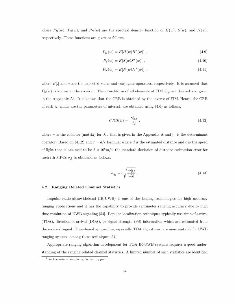
where PH(w), PS(w), and PN (w) are the spectral density function of H(w), S(w), and N(w),
respectively. These functions are given as follows,
PH(w) = E[H(w)H∗(w)] , (4.9)
PS(w) = E[S(w)S∗(w)] , (4.10)
PN (w) = E[N(w)N∗(w)] , (4.11)
where E[.] and ∗ are the expected value and conjugate operators, respectively. It is assumed that
PS(w) is known at the receiver. The closed-form of all elements of FIM Jxy are derived and given
in the Appendix A1. It is known that the CRB is obtained by the inverse of FIM. Hence, the CRB
of each τl, which are the parameters of interest, are obtained using (4.6) as follows,
CRB(τl) =[γ]l,l|Jθ| , (4.12)
where γ is the cofactor (matrix) for Jττ that is given in the Appendix A and |.| is the determinant
operator. Based on (4.12) and τ = d/c formula, where d is the estimated distance and c is the speed
of light that is assumed to be 3 × 10⁸m/s, the standard deviation of distance estimation error for
each lth MPCs σdlis obtained as follows,
σdl= c
√[γ]l,l|Jθ| . (4.13)
4.2 Ranging Related Channel Statistics
Impulse radio-ultrawideband (IR-UWB) is one of the leading technologies for high accuracy
ranging applications and it has the capability to provide centimeter ranging accuracy due to high
time resolution of UWB signaling [54]. Popular localization techniques typically use time-of-arrival
(TOA), direction-of-arrival (DOA), or signal-strength (SS) information which are estimated from
the received signal. Time-based approaches, especially TOA algorithms, are more suitable for UWB
ranging systems among these techniques [54].
Appropriate ranging algorithm development for TOA IR-UWB systems requires a good under-
standing of the ranging related channel statistics. A limited number of such statistics are identified1For the sake of simplicity, ’w’ is dropped.
54

for specific algorithms and modeled using measurement data in [77], [78], [79] and some of IEEE
802.15.4a channel models in [80]. In [77], a TOA ranging scheme using UWB radio link is proposed.
Relative path strength and the delay between the strongest and direct paths are two critical pa-
rameters used for the proposed algorithm. These parameters are modeled statistically using a set of
propagation measurements. In [78], some frequency domain measurements are performed for indoor
geolocation applications (especially for WLAN applications) to measure the TOA of the first path.
By using the data from the measurements, the effects of sampling period of radio channel (in both
time and frequency domain), multipath and filtering on the accuracy of the distance estimation are
studied.
In [79], the impact of some of the standard channel parameters on the performance of various
UWB transmission schemes such as Rake receivers and Transmitted-reference (TR) systems are
discussed briefly without providing analytical or simulation results. Furthermore, the effects of
different receiver structures such as Stored-reference (SR) systems, TR and Energy detectors (ED)
on the performance of TOA IR-UWB systems are analyzed and evaluated for CM1 and CM2 channel
models of IEEE 802.15.4a standard in [81].
The previous studies motivate us to develop and study a unified list of TOA ranging related
channel parameters and their statistics. Hence, in this section, we identify and investigate such
parameters that have an impact on TOA IR-UWB ranging and obtain their statistics using computer
simulations. The effects of the IEEE 802.15.4a channel models that represent different channel
environments are discussed and impact of different type of receivers on these parameters are studied.
The discrete-time complex baseband channel impulse response (CIR) of IEEE 802.15.4a channel
models is given in general as [82]
h[n] =L∑
l=0
K∑
k=0
ak,lejφk,lδ[n− Tl − τk,l] , (4.14)
where ak,l is the tap coefficient of the kth multipath component (MPC) in the lth cluster, Tl is the
delay of the lth cluster, τk,l is the delay of the kth multipath component relative to the lth cluster
arrival time Tl. The phases are denoted as φk,l and it is a uniformly distributed random variable
within the range of [0, 2π]. The number of clusters and MPCs are denoted as L and K, respectively.
In order to obtain the distance between a transmitter and a receiver in TOA ranging techniques,
time delay information of the first arriving path is used. The algorithms that search for the first
55

arriving path typically start the search from the strongest path [77, 80]; therefore, the paths prior
to the strongest path are candidates for the leading edge of the signal. For the sake of discussion,
let the discrete-time representation of the first arriving path and strongest path be denoted as the
leading edge sample (LES) and peak sample (PS), respectively. It is assumed that the CIR has finite
number of taps (n = 0, 1, ..., N − 1). The index of the LES (nle), which is the index of the first tap,
is then given by
nle = min{
n∣∣h[n] 6= 0
}, (4.15)
The PS is defined as the tap with maximum coefficient. Consequently, the index of PS is given by
np = argmaxn
{h[n]
}. (4.16)
4.2.1 IEEE 802.15.4a Channel Models
Detection of the first arriving path and the ranging accuracy highly depends on the multipath
channel characteristics. Extensive research have been carried out in the past in order to model
the UWB CIR in (4.14) for different environments. While IEEE802.15.3a channel models [83]
are the first standardized channel models for UWB systems, a more comprehensive set of channel
models was recently developed under the IEEE 802.15.4a standardization group [82]. The latter
standard provides nine different channel models for different environments including LOS and NLOS
scenarios [82], which are shown in Table 4.2. A comparison of both channel models can be found
in [79] and a more detailed information for each IEEE 802.15.4a channel model such as range coverage
and frequency range is reported in [82].
The IEEE 802.15.4a standard channel models have few important characteristics that are very
critical for UWB ranging applications [84]. One of these characteristics is the frequency-dependent
path loss, which indicates that the distortion of each separate multipath component depends on the
frequency. Hence, the operating frequency used at transmitter affects the ranging related channel
statistics. Another important characteristics that is specific to the office NLOS (CM4) and industrial
NLOS (CM8) channel models is the ”soft” onset concept. Due to the ”soft” onset, the first arriving
paths can be significantly weaker than the later MPCs in a power delay profile [84]. This implies
that the detection of the first arriving path can be very challenging in such scenarios.
56

4.2.2 The Effects of Receiver Architectures
Although numerous types of receiver architectures are proposed for UWB communications sys-
tems in the literature, non-coherent receivers are suitable for low-complexity UWB ranging applica-
tions [81].
The statistics of ranging related parameters are affected by the employed receiver type. In this
section, we consider the following three cases to study ranging related channel statistics:
• Channel impulse response (CIR): The statistics of ranging related parameters can be obtained
directly from the CIR in (4.14) (i.e. sampled at Nyquist rate). Such an analysis may be
particularly useful for coherent ranging such as using Rake receivers.
• Energy block (EB): In order to analyze the ranging related statistics when using TR (differ-
entially coherent) and ED (non-coherent) types of receivers, the CIR in (4.14) can be passed
through a square-law device and sampled at a practical sampling rate (i.e. path energies are
aggregated within energy blocks). In this case, the sampling rate is much lower than that of
CIR case.
• Energy block with waveform effects (EBWF): In order to model a more practical case, the
CIR in (4.14) can be convolved with a practical pulse shape before passing the signal through
a square-law device and sampling it. This captures the inter-pulse interference between the
different multipath components and resulting statistics depend on the employed pulse shape.
Apart from the employed receiver type, there are few other receiver-related factors that may
have impacts on ranging-related channel statistics.
• Antenna has an impact on the statistical parameters of ranging applications due to frequency
dependence of the antenna characteristics.
• Filtering operations in the receiver chain may also affect the ranging related channel statistics.
Since filtering introduces side-lobes prior to the leading edge of the signal (in time domain),
the filtering effects may yield additional distance estimation errors [78]. Hence, mitigation of
filtering effects is required at the receiver in order to improve TOA ranging accuracy.
Noise level and multiuser interference [54] are some other parameters that may have effects on
ranging related channel statistics.
57

4.2.3 Channel Statistics for Practical TOA Ranging Algorithms
The illustration of channel statistics for practical TOA estimation is shown in Fig. 4.1. The
following ranging related channel statistics are identified based on three parameters in (4.14), which
are amplitude, phase and delay of MPCs.FrameStart FrameEndSample Indexnle npEle EpClusterDelayBetweenClusters Noise blockEnergy+Noise block Threshold
Figure 4.1 Illustration of time of arrival (TOA) ranging related channel statistics.
4.2.3.1 Statistics of Amplitude and Phase of the Leading Edge and Peak Samples
These statistics are helpful for setting a threshold to detect LES and for the identification of line-
of-sight (LOS) and non-line-of-sight (NLOS) environments. The accuracy of the ranging algorithm
can be improved with the knowledge of these statistics since the leading edge detection threshold and
searchback window length [80] (or the search stopping rule [77]) can be determined more accurately.
The phase statistics can be useful for coherent ranging systems.
The energy of the LES (Ele) and PS (Ep) are two important parameters that affect ranging
accuracy. In this section, we will analyze the mean energy of the LES (Ele) and PS (Ep) rather than
the complete statistics of the amplitude and phase.
4.2.3.2 Statistics of the Delay Between the Leading Edge and Peak Samples
Delay between the peak and the leading edge samples (τple) can be useful for determining the
complexity and accuracy of search algorithms and for identifying the LOS and NLOS environments.
58

4.2.3.3 Statistics of Number of Clusters Prior to the Peak Sample
Number of clusters prior to the peak sample (Λ) is an important statistical parameter, since it
determines the number of noise-only clusters between signal clusters and thus may have an impact
on threshold selection. This may affect the performance of certain searchback algorithms [85].
4.2.3.4 Statistics of Number of Delays Between Clusters that are Prior to the Peak
Sample
Number of delays between clusters that are prior to the peak sample (γ) is also important for
setting a threshold in certain searchback algorithms. The statistical information of the noise samples
prior to the LES can also affect the performance of search algorithms [85].
In addition to above statistics, the power delay profiles (PDP) of different channel models, and
the probability density function (PDF) of the energy within different samples are other important
statistics which may have effects on the ranging algorithms (however, they will not be analyzed
further in this dissertation).
4.2.4 Results and Discussions
Due to the nature of DSASs, the utilized spectrum parameters such as absolute bandwidth B and
operating center frequency fc can be dynamic. Furthermore, channel environment can be dynamic
as well. Therefore, the effects of these parameters on σd are investigated in this section. Since the
channel models developed by IEEE 802.15.4a standard group [82] take the FDF-MPCs into account,
the parameters (α, φ, β) of these channel models are used to obtain the results in this section.
In this standard, Fl(w) is modeled as w−2κ, where κ is the frequency dependency of the channel
environment. In this model, it is assumed that all the MPCs in a channel environment (e.g. indoor
residential LOS) have the same FDPC, which is βl = −2κ. However, each channel environment has
different κ, which is shown in Table 4.1. Moreover, Gaussian second derivative pulse shape with the
duration of 2ns is considered.
The impacts of B on σd is studied and the results are plotted in Fig. 4.2 (Top figure: κ = 1.12,
fc = 6GHz, CM1 channel model parameters [82]). According to the results, increasing B improve
the ranging accuracy even in the presence of FDF-MPCs. For instance, increasing B from 600MHz
to 1000MHz improves the ranging accuracy from 5.53m to 46cm at −8dB SNR level. Similarly, the
effects of fc on σd is investigated and the results are shown in Fig. 4.2 (Bottom figure: κ = 0.12,
59

Table 4.1 The measured κ values of some UWB channels.Channel Models κCM1 (Residential Indoor LOS) 1.12CM2 (Residential Indoor NLOS) 1.53CM3 (Office Indoor LOS) 0.03CM4 (Office Indoor NLOS) 0.71CM5 (Outdoor LOS) 0.12CM6 (Outdoor NLOS) 0.13CM7 (Industrial LOS) -1.103CM8 (Industrial NLOS) -1.427
B = 500MHz, CM5 channel model parameters [82]). The results show that increasing fc deteriorates
the ranging accuracy. For instance, ranging accuracy degradation due to operating at fc = 3.5GHz
rather than fc = 2.5GHz is approximately 1.75m at the SNR level of −8dB. The additional path loss
that occurs at higher center frequencies due to the FDF-MPCs reduces the probability of detection
of the first arrival paths and this causes a degradation in the ranging accuracy.
The effects of FDF-MPCs on the σd are investigated as well and the results are shown in
Fig. 4.3 (B = 500MHz, fc = 6GHz, CM1 channel model parameters [82]). According to the re-
sults, the parameter κ is inversely proportional to σd. This implies that the ranging accuracy in
−10 −5 0 5 10−2
−1.5
−1
−0.5
0
0.5
1
1.5
SNR [dB]
σ d [m]
B=600 MHzB=800 MHzB=1000 MHz
−10 −5 0 5 10 15−2.5
−2
−1.5
−1
−0.5
0
0.5
1
SNR [dB]
σ d [m]
fc= 2.5 GHz
fc= 3 GHz
fc=3.5 GHz
Figure 4.2 The effects of absolute bandwidth (top figure) and center frequency (bottom figure) onthe standard deviation of the distance estimation error in log scale.
60

−12 −10 −8 −6 −4 −2 0 2 4 6 8−2
−1.5
−1
−0.5
0
0.5
1
1.5
SNR [dB]
σ d [m]
κ=0κ=1.06κ=1.12κ=1.18
Figure 4.3 The effects of frequency dependency of the channel environment on the standard deviationof the distance estimation error in log scale.
highly frequency-dependent channel environments is worse than that of low frequency-dependent
channel environments under the same conditions. For instance, the ranging accuracy is 5.88m for
the channel with κ = 1.18 whereas the ranging accuracy is 4.3m for the channel with κ = 1.06 at
−8dB SNR level. The reason behind this result is the reduction in the detection probability of the
first arrival MPCs due to the frequency dependency of the channel. Moreover, Fig. 4.3 contains a
curve for κ = 0 case that represents the propagation channel without FDF-MPCs. As it can be seen
clearly, FDF-MPCs shifts up the bound significantly (5.6m for κ = 1.18 at −8dB SNR level). Hence,
the effects of FDPG on the accuracy of TOA ranging algorithms can be significant depending on
the frequency-dependent feature of the radio channel. Note that the results in all three figures have
a common trend, which is the proportionality between the ranging accuracy and the SNR level.
We investigate the statistics of Ep, Ele, τple, Λ, and γ through computer simulations. The results
are obtained over 2000 different channel realizations for each channel model. Center frequency of
6GHz is used during the generation of all channel models. The sampling times that are used during
simulations for CIR, EB, and EBWF cases are 0.1265ns, 3.79ns, and 3.79ns, respectively. For the
third case, a root raised cosine (RRC) pulse with parameters α = 0.5, B = 500MHz, and pulse
61

Table 4.2 The τple values in ns for different channel models that have a probability of 5 · 10−4.
Channel Models CIR EB EBWFCM1 (Residential Indoor LOS) 59 61 55CM2 (Residential Indoor NLOS) 83 87 91CM3 (Office Indoor LOS) 42 34 53CM4 (Office Indoor NLOS) 38 38 44CM5 (Outdoor LOS) 127 91 99CM6 (Outdoor NLOS) 380 342 380CM7 (Industrial LOS) 27 23 46CM8 (Industrial NLOS) 228 154 213CM9 (Open Outdoor NLOS) 228 222 228
Table 4.3 The values of Ep and Ele for different channel models.
Channel CIR EBEp Ele Ep Ele
CM1 164 · 10−3 129 · 10−3 419 · 10−3 338 · 10−3
CM2 73.6 · 10−3 0.76 · 10−3 304 · 10−3 68 · 10−3
CM3 131 · 10−3 63 · 10−3 449 · 10−3 422 · 10−3
CM4 52 · 10−3 11 · 10−3 230 · 10−3 139 · 10−3
CM5 114 · 10−3 55 · 10−3 368 · 10−3 317 · 10−3
CM6 76 · 10−3 0.11 · 10−3 182 · 10−3 7.9 · 10−3
CM7 181 · 10−3 104 · 10−3 739 · 10−3 725 · 10−3
CM8 782 · 10−5 2.3 · 10−5 4098 · 10−5 325 · 10−5
CM9 398 · 10−3 1.1 · 10−3 654 · 10−3 60.6 · 10−3
duration of 4ns are used. The effects of antennas, filters, and noise level are not included in the
simulations.
The Ep and Ele values for all nine channel models and for CIR and EB cases are tabulated in
Table 4.3. For all channel models, the Ep and Ele values of EB case are larger than those of CIR
case due to aggregation of path energies within the block duration. Although using energy blocks
increases the energy of both LES and PS, the noise energy also increases in practice. Nevertheless,
aggregation of path energies within block duration may increase the probability of detection of both
LES and PS. This advantage comes with the cost of an additional error in accuracy of distance
estimation due to decrease in the path resolution. Ep and Ele values of all LOS channels for both
CIR and EB cases are larger than those of corresponding NLOS channels. These results indicate
that detection of both LES and PS in LOS environments are easier than NLOS ones. The CM7-EB
and CM8-CIR cases have the largest and lowest Ele values, respectively.
62

0 0.1 0.2 0.3 0.4 0.5 0.6 0.7 0.80
0.1
0.2
0.3
0.4
0.5
Delay (ns)P
DF
CM1CM3CM5CM7
0 10 20 30 40 50 60 70 800
0.002
0.004
0.006
0.008
0.01
Delay (ns)
PD
F
CM2CM4CM6CM8CM9
CM8
CM4
Figure 4.4 The statistics of the delay between the peak and leading edge sample (τple) based onchannel impulse response for line of sight (LOS) and non-line of sight (NLOS) environments.
The PDFs of τple for CIR and EB for all the channel models are presented in Fig. 4.4 and 4.5
where we used 10th order polynomial curve fits to smooth the results. Also, the values of τple that
has a probability of 5 · 10−4 for all the cases are tabulated in Table 4.2. According to Fig. 4.4,
minimum value of τple is 0ns for all channels. For the CIR case, CM1 and CM8 are the channels
that have the highest and lowest probability for τple = 0 (i.e. PS is the LES), respectively. This
implies that CM1 has the highest probability that the first arriving path is the strongest path, which
is desirable for ranging applications. For CM8 channel, the probability of the first arriving path to
be the strongest path is about zero. This is due to the first arriving paths of CM8 being very weak
(soft onset effects). For the CIR case, maximum and minimum upper limit of τple are observed for
CM6 (380ns) and CM7 (27ns), respectively. It is concluded that the most complex and the least
complex search algorithms (in terms of timing estimation) will be required most likely for CM8 and
CM7 channels, respectively.
According to Fig. 4.5, the probability of τple being zero for all channels in EB case are larger than
those in CIR case. This is due to the reduction of delays during the aggregation of path energies
within the blocks. This also comes with an additional error in accuracy.
63

0 1 2 3 4 5 6 7 80
0.2
0.4
0.6
0.8
1
Delay (ns)P
DF
0 10 20 30 40 50 60 70 800
0.1
0.2
0.3
0.4
Delay (ns)
PD
F
CM2CM4CM6CM8CM9
CM1CM3CM5CM7
Figure 4.5 The statistics of the delay between the peak and leading edge sample (τple) based onenergy block for line of sight (LOS) and non-line of sight (NLOS) environments.
For the EB case, maximum and minimum values of τple that has a probability of 5 · 10−4 are
for CM6 (342ns) and CM7 (23ns) channels, respectively. The results suggest that the block length
affects the τple statistics and consequently the complexity of the search algorithm.
Results obtained for EBWF are similar to those in EB case. The probability of τple being zero for
all channels in EBWF case are slightly lower than those in EB case. In the case of EBWF, maximum
and minimum upper limit of τple are observed for CM6 (380ns) and CM4 (44ns), respectively.
Therefore, the effects of waveform on the τple statistics is not significant.
The PDFs of Λ and γ for all LOS and NLOS channels are plotted in Figs. 4.6 and 4.7, respectively.
The probability of Λ being zero for CM3, CM4, CM7, and CM8 are approximately 100%. According
to [82], CM4 and CM8 channels have a single power delay profile (single cluster), which agree with
our results. Maximum value of Λ for CM1, CM2, CM5, CM6, and CM9 channels are 1, 2, 1, 5, and
3, respectively. Overall, the number of clusters for the LOS channels are equal or less than those for
the NLOS channels. For all channels except CM8 channel, the γ value with the highest probability
is 3.79ns. In the case of CM8 channel, the probability of γ statistics for all possible delay values is
zero. Maximum possible delay value for CM1, CM2, CM3, CM4, CM5, CM6, CM7, CM8, and CM9
channels are 22.74, 18.95, 18.95, 18.95, 37.9, 41.69, 18.95, 0, and 56.85ns, respectively.
64
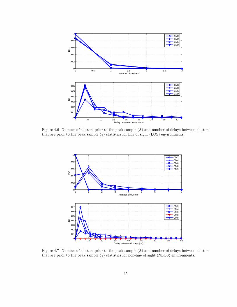
0 0.5 1 1.5 2 2.5 30
0.2
0.4
0.6
0.8
1
PD
F
Number of clusters
0 5 10 15 20 25 30 35 400
0.1
0.2
0.3
0.4
0.5
0.6
PD
F
Delay between clusters (ns)
CM1CM3CM5CM7
CM1CM3CM5CM7
Figure 4.6 Number of clusters prior to the peak sample (Λ) and number of delays between clustersthat are prior to the peak sample (γ) statistics for line of sight (LOS) environments.
0 1 2 3 4 5 6 7 80
0.2
0.4
0.6
0.8
1
PD
F
Number of clusters
CM2CM4CM6CM8CM9
0 10 20 30 40 50 60 70 800
0.1
0.2
0.3
0.4
0.5
0.6
0.7
PD
F
Delay between clusters (ns)
CM2CM4CM6CM8CM9
Figure 4.7 Number of clusters prior to the peak sample (Λ) and number of delays between clustersthat are prior to the peak sample (γ) statistics for non-line of sight (NLOS) environments.
65

4.3 Conclusions
The performance analysis of TOA IR-UWB high accuracy ranging algorithm for the DSASs is
carried out. The general expression of asymptotic frequency-domain CRB for the ranging algorithm,
which takes the FDF-MPCs and phase information into account, is derived through Whittle For-
mula. The impacts of the FDF-MPCs, absolute bandwidth, and operating center frequency on the
ranging accuracy are investigated. The results reveal the necessity of including FDF-MPCs into
the performance analysis of TOA ranging algorithms and it is suggested to utilize as large absolute
bandwidth as possible at low center frequencies in order to achieve high precision ranging in the
DSASs.
In addition, a list of channel statistics specific to the ranging applications employing TOA IR-
UWB systems are presented. The statistics are obtained via computer simulations by considering the
impacts of different channel environments and as well as receiver structures. The results suggest that
different channel environments and receivers affect the ranging related channel statistics significantly.
The effects of operating frequency, antenna, filtering, and noise level on the statistics can be studied
further.
66
CHAPTER 5
TIME DELAY ESTIMATION USING DISPERSED SPECTRUM UTILIZATIONAPPROACH
5.1 Introduction
One of the prominent characteristics of cognitive radio [9], [10], [20] is location awareness [2], [15],
[24]. Cognitive radios with location awareness cycle [15] can support goal driven and autonomous
location aware systems such as location-based services (e.g., package tracking), location-assisted net-
work optimization (e.g., dynamic spectrum management), location-assisted transceiver optimization
(e.g., adaptive beamforming), and location-assisted environment identification (e.g., propagation
channel characterization), which are discussed in Chapter 7.
A conceptual architecture for cognitive radio with a location awareness cycle, which consists of
a location awareness engine, sensing interface and environment loop, is presented in Chapter 2 [15].
In the same chapter [2], a conceptual model for the location awareness engine, which is the main
component of a location awareness cycle, is introduced. The main tasks of the location awareness
engine are location sensing, seamless positioning and interoperability, security and privacy, statisti-
cal learning and tracking, mobility management, adaptation of location aware systems, and location
aware applications [2], [15]. In order to develop a location sensing method for the location awareness
engine, a cognitive positioning system (CPS) along with range accuracy adaptation method is pro-
posed in Chapter 3 [12], [16]. The CPSs use Cramer-Rao lower bound (CRLB) information at the
transmitter side to optimize the transmission parameters for achieving goal driven range and posi-
tion accuracy requirements. In Chapter 3, the CRLB for time delay estimation in both AWGN and
multipath channels are derived, where the path delays and coefficients are assumed to be unknown.
This analysis is extended in Chapter 4 by deriving the frequency-domain CRB in dynamic spectrum
access systems. In Chapter 4, it is assumed that path delays, distance-dependent coefficients, phases
and frequency-dependent coefficients are unknown. Furthermore, the effects of bandwidth, carrier
frequency, and path frequency dependence on the CRLB in dynamic spectrum access systems are
67

investigated. Note that the studies in Chapters 3 and 4 are based on the fact that the available
bandwidth is in the form of a single piece (i.e., the whole bandwidth). Since the available band-
widths in the dynamic spectrum access systems are dispersed [86], a single cognitive radio user can
transmit and receive over multiple dispersed bands. Such method is referred as dispersed spectrum
utilization systems and developed in the context of time delay estimation in this chapter.
In this chapter, fundamental limits of time delay estimation are studied in dispersed spectrum
utilization systems, where the available dispersed bandwidths are assumed to be narrow. The limits
are quantified in terms of the CRLBs and the effects of both unknown channel coefficients and
carrier frequency offsets (CFOs) are taken into account. After deriving a generic expression, specific
CRLB formulas are obtained for various modulation schemes1. It is shown for linear modulation
schemes that the same fundamental limits can be achieved for the cases of known and unknown
CFOs. In addition, it is proven that the effects of unknown channel coefficients are mitigated as well
for linear modulations with constant envelopes. Finally, numerical results are presented to verify
the theoretical analysis.
5.2 Signal Model
Consider a cognitive radio system that occupies K different frequency bands as shown in Fig.
5.1. The cognitive transmitter sends a signal occupying all the K bands, and the receiver wishes
to calculate the time delay of the incoming signal. One way to implement such a system is to
consider the received signal as an orthogonal frequency division multiplexing (OFDM) signal with
zero coefficients at the sub-carriers corresponding to the unused bands [87], [88], [89]. Then, the
signal can be processed as in a conventional OFDM receiver. However, the available spectrum can
be very dispersed in some cases, which requires processing of very large bandwidths if the signal is
considered as a single OFDM signal. In such cases, it can be more practical to process the signal
in multiple branches, as shown in Fig. 5.2. Each branch considers one available band, and down-
converts the signal according to the center frequency of that band. In this way, signals with narrower
bandwidths can be processed at each branch. Then, the question is to determine the accuracy of
time delay estimation for such a receiver structure, considering practical issues such as CFO due to
the use of multiple down-conversion units.1The author thanks to Dr. Sinan Gezici for his contributions to this chapter, especially for the development of
Sections 5.3 and 5.4.
68

Frequency….
PSDfc1 fc2 fcKB1 BKB2
UnavailableBandsFigure 5.1 Illustration of dispersed spectrum utilization in cognitive radio systems.
The baseband representation of the received signal in the ith branch can be expressed as
ri(t) = αie−jωitsi(t− τ) + ni(t) , (5.1)
for i = 1, . . . , K, where αi = aiejφi and ωi represent, respectively, the channel coefficient and
the CFO for the signal in the ith branch, si(t) is the baseband representation of the transmitted
signal corresponding to the ith band, τ is the time delay, and ni(t) is complex Gaussian noise with
independent and white components, each having spectral density σ2i .
For the signal model in (5.1), it is assumed that the signal at each branch can be modeled as a
narrowband signal. Therefore, a single complex channel coefficient is used to represent the fading
of each signal.
Note that, in addition to the cognitive radio framework, the signal model in (5.1) can also
represent a multiple-input multiple-output (MIMO) system, in which transmitter i sends si(t) to
receiver i, in the presence of synchronization among the transmissions, or when the receiver knows
the relative delays between transmissions.
5.3 CRLB Calculations
Let θ = [τ a1 · · · aK φ1 · · ·φK ω1 · · ·ωK ] represent the vector of unknown signal parameters. If
the signals in (5.1) are observed over the interval [0, T ], the log-likelihood function for θ is given
69

fc1B1PSD ffc2B2PSD f
fcKBKPSD f... ...
r1(t)fc1r2(t)fc2rK(t)fcK
DownconversionLNABPF1DownconversionLNABPF2DownconversionLNABPFK
Figure 5.2 Block diagram of a cognitive radio receiver.
by [56]
Λ(θ) = c−K∑
i=1
12σ2
i
∫ T
0
∣∣ri(t)− αiejωitsi(t− τ)∣∣2 dt , (5.2)
where c is a constant that is independent of θ. Then, the maximum likelihood (ML) estimate for θ
can be obtained from (5.2) as2
θML = arg maxθ
{K∑
i=1
1σ2
i
∫ T
0
R{α∗i e
−jωitri(t)s∗i (t− τ)}
dt−K∑
i=1
Ei|αi|22σ2
i
}, (5.3)
2For a complex number z, R{z} and I{z} represent its real and imaginary parts, respectively.
70

where Ei =∫ T
0|si(t − τ)|2dt is the signal energy3. From (5.2), the Fisher information matrix
(FIM) [56] can be obtained, after some manipulation, as
I =
Iττ Iτa Iτφ Iτω
ITτa Iaa 0 0
ITτφ 0 Iφφ Iφω
ITτω 0 IT
φω Iωω
, (5.4)
with
Iττ =K∑
i=1
γiEi , (5.5)
Iaa = diag{
E1
σ21
, . . . ,EK
σ2N
}, (5.6)
Iφφ = diag {E1γ1, . . . , EKγK} , (5.7)
Iωω = diag {F1γ1, . . . , FKγK} , (5.8)
Iτa = −[ER
1
|α1|σ2
1
· · · ERK
|αK |σ2
K
], (5.9)
Iτφ = −[EI
1γ1 · · · EIKγK
], (5.10)
Iτω = − [G1γ1 · · · GKγK ] , (5.11)
Iφω = diag{
F1γ1, . . . , FKγK
}, (5.12)
where γi = |αi|2/σ2i , diag{x1, . . . , xK} represents an K ×K diagonal matrix with its ith diagonal
being equal to xi, Ei is the energy of the first derivative of si(t); i.e., Ei =∫ T
0|s′i(t− τ)|2 dt, and
ERi , EI
i , Fi, Fi and Gi are given, respectively, by
ERi =
∫ T
0
R{s′i(t− τ)s∗i (t− τ)}dt , (5.13)
EIi =
∫ T
0
I {s′i(t− τ)s∗i (t− τ)}dt , (5.14)
Fi =∫ T
0
t2 |si(t− τ)|2 dt , (5.15)
Fi =∫ T
0
t |si(t− τ)|2 dt , (5.16)
Gi =∫ T
0
t I {s∗i (t− τ)s′i(t− τ)}dt . (5.17)
3Although Ei is a function of τ in general, it is not shown explicitly for convenience. The same convention is alsoemployed for the expressions in (5.13)-(5.17).
71

The CRLB for unbiased time delay estimators can be obtained from the element in the first row
and first column of the inverse of the FIM in (5.4), i.e.,[I−1
]11
. Based on the formulas for block
matrix inversion, the CRLB can be obtained as (Appendix B)
CRLB1 =1
∑Ki=1 γi
(Ei − (ER
i )2/Ei
)− ξ
, (5.18)
where
ξ =K∑
i=1
γi(EI
i)2Fi + EiG
2i − 2EI
iGiFi
EiFi − F 2i
. (5.19)
In order to investigate the effects of unknown CFOs, the CRLB for time delay estimation
can be obtained for known CFOs. In that case, the unknown parameter vector reduces to θ =
[τ a1 · · · aK φ1 · · ·φK ], and the CRLB can be obtained, similarly to the previous derivations, as
CRLB2 =1
∑Ki=1 γi
(Ei − E2
i /Ei
) , (5.20)
where
Ei =∣∣∣∣∫ ∞
−∞s′i(t− τ)s∗i (t− τ)dt
∣∣∣∣ =√
(ERi )2 + (EI
i)2 . (5.21)
Note that CRLB2 in (5.20) is smaller than or equal to CRLB1 in (5.18) in general, since more
unknown parameters exist for the latter.
If both the channel coefficients and the CFOs are known, the unknown parameter vector reduces
to τ . Then, the CRLB can be obtained from (5.5) as
CRLB3 =1∑K
i=1 γiEi
. (5.22)
5.4 Special Cases
Although the CRLB can be obtained from (5.13)-(5.19) in general, its evaluation for specific
signal structures can provide more intuition related to the effects of CFOs.
72

Let consider the baseband signal si(t) in (5.1) to be composed of a sequence of modulated pulses
as follows:
si(t) =∑
l
di,l(t)pi(t− lTi) , (5.23)
for i = 1, . . . , K, where di,l(t) denotes the complex data4 for the lth symbol of signal i, and pi(t)
represents a pulse with duration Ti, i.e., pi(t) = 0 for t 6∈ [0, Ti]. To simplify notation, it is assumed
that the observation interval T can be expressed as T = NiTi for an integer Ni for i = 1, . . . , K.
• Proposition 1: For any linear modulation of the form si(t) =∑
l di,lpi(t− lTi), the CRLBs in
(5.18) and (5.20) are equal, and are given by
CRLB1 = CRLB2 =1
∑Ki=1 γi
(Ei − (ER
i )2/Ei
) . (5.24)
• Proof: When the complex data di,l(t) is not time-dependent, as stated in the proposition,
s′i(t)s∗i (t) can be calculated from (6.5) as
s′i(t)s∗i (t) =
∑
l
|di,l|2pi(t− lTi)p′i(t− lTi) . (5.25)
Since s′i(t)s∗i (t) is a real quantity, it can be shown that EI
i in (5.14) and Gi in (5.17) are equal
to zero. Therefore, it can be observed from (5.19) and (5.21) that CRLB1 in (5.18) and CRLB2
in (5.20) reduce to the expression stated in the proposition. ¤
Proposition 1 states that for most modulation types, such as pulse amplitude modulation
(PAM), phase shift keying (PSK) and quadrature amplitude modulation (QAM) [90], the
CRLB of time delay estimation for the case of unknown CFOs is the same as that for the case
of known CFOs5. For non-linear modulation types, the statement in the proposition cannot
be employed. For example, for FSK modulation with di,l(t) = exp{
j2πdi,l∆it}, where di,l is
the modulation data and ∆i is the amount of frequency shift, EIi in (5.14) and Gi in (5.17)
are not zero in general.4Since a data-aided time delay estimation scenario is considered, the data symbols are assumed to be known.5Unknown channel coefficients are considered for both cases.
73

• Proposition 2: For linear modulations of the form si(t) =∑
l di,lpi(t − lTi), with |di,l| = |di|∀l and pi(t) satisfying pi(0) = pi(Ti) for i = 1, . . . , K, the CRLBs in (5.18), (5.20) and (5.22)
are given by
CRLB1 = CRLB2 = CRLB3 =1
4π2∑K
i=1 SNRiβ2i
, (5.26)
where SNRi = Ni|di|2 |αi|2Epi
σ2i
with Epi=
∫∞−∞ p2
i (t)dt, and βi is the effective bandwidth of
pi(t), given by
β2i =
1Epi
∫ ∞
−∞f2|Pi(f)|2df , (5.27)
with Pi(f) denoting the Fourier transform of pi(t).
• Proof: Since |di,l| = |di| ∀l, ERi in (5.13) can be obtained from (5.25) as
ERi = |di|2
∑
l
∫ T
0
pi(t− τ − lTi)p′i(t− τ − lTi)dt (5.28)
= Ni|di|2∫ ∞
−∞pi(t)p′i(t)dt = 0 , (5.29)
for i = 1, . . . , K. Note that the second equality is obtained from the fact that T = NiTi, and
the final equality is due to the facts that pi(t) is non-zero only over t ∈ [0, Ti] and satisfies
pi(0) = pi(Ti).
Since ERi = 0 for i = 1, . . . , K, the CRLB expression in (5.24) becomes
CRLB1 = CRLB2 =1∑K
i=1 γiEi
, (5.30)
which is the same as the CRLB in (5.22) for the case of known CFOs and channel coefficients.
In addition, Ei can be calculated, from (6.5) and the fact that |di,l| = |di| ∀l, as
Ei =∫ T
0
|s′i(t− τ)|2dt = |di|2∑
l
∫ T
0
(p′i(t− τ − lTi))2 dt = Ni|di|2Epi , (5.31)
where Epi =∫∞−∞ (p′i(t))
2 dt. From Parseval’s relation, Epi can be expressed as 4π2β2i Epi ,
where Epi is the energy of pi(t) and βi is the effective bandwidth of pi(t) [56]. In what
74

follows, it is observed from (5.31) that (5.30) is equal to (5.26) for SNRi = Ni|di|2γiEpiand
γi = |αi|2/σ2i . ¤
From Proposition 2, it is observed that for linear modulations with constant envelope, such as
PSK, the CRLB for time delay estimation is the same whether the CFOs and/or channel coefficients
are known or unknown for pulses satisfying p(0) = p(T ), which is usually the case in practice.
This implies that in such cases, the ML estimators in the absence of any information on CFOs and
channel coefficients can asymptotically achieve the same CRLB as the ones in presence of CFO
and/or channel coefficient information [56].
5.5 Numerical Results
In this section, numerical studies are described that illustrate the CRLBs discussed in Sections 5.3
and 5.4. It is assumed that all the K bands in the system have the same bandwidth and the same
pulse is employed for all of them; i.e., pi(t) = p(t) for i = 1, . . . ,K (c.f. (6.5)). For the pulse shape,
the following Gaussian second order derivative is employed
p(t) = A
(1− 4πt2
ζ2
)e−2πt2/ζ2
, (5.32)
where A and ζ are parameters that are used to adjust the pulse energy and the pulse width, respec-
tively. In the following, ζ = 1 µs is employed, for which the pulse width becomes approximately 2.5
µs, and A is selected in order to generate pulses with unit energy. In addition, it is assumed that
the spectral density of the noise is the same for all the K branches; i.e., σi = σ for i = 1, . . . ,K, and
the system SNR is defined as the sum of the SNRs in the various branches.
In Fig. 5.3, the CRLB expressions in (5.18), (5.20) and (5.22), labeled as CRLB1, CRLB2 and
CRLB3, respectively, are plotted versus SNR for three different modulation types, namely 16FSK6,
16QAM, and 16PSK. For all cases, it is assumed that the same modulation sequence is used at dif-
ferent branches; i.e., di,l(t) = dl(t) for i = 1, . . . ,K, and that the channel amplitudes are normalized
to unity; i.e., |αi| = 1 for i = 1, . . . , K. In addition, the modulation sequence for each modulation
type is scaled appropriately so that the sequences have the same energy in all cases. Also, there
are K = 3 branches in the system, and N = 2 symbols are received at each branch. From the
figure, it is first observed that for all the modulations, CRLB3 ≤ CRLB2 ≤ CRLB1 is satisfied,
since CRLB1 corresponds to the case of unknown delay, channel coefficients and CFOs, CRLB2
6The amount of frequency shift is selected as 190 kHz for the FSK modulation.
75

0 2 4 6 8 10 12 14 16 18 20
10−7
10−6
SNR [dB]
√
CR
LB
[sec
]
16PSK−CRLB116PSK−CRLB216PSK−CRLB316QAM−CRLB116QAM−CRLB216QAM−CRLB316FSK−CRLB116FSK−CRLB216FSK−CRLB3
Figure 5.3√
CRLB versus SNR for K = 3 and N = 2.
corresponds to the case of unknown delay and channel coefficients, and CRLB3 corresponds to the
case of unknown delay only. In other words, for the cases with fewer unknown parameters, lower
CRLBs are observed. For the 16FSK modulation, all three bounds are distinct, which is possible
because 16FSK is a non-linear modulation and the result of Proposition 1 does not apply in this
case. For the 16QAM case, CRLB1 = CRLB2 as expected from Proposition 1. However, CRLB3 is
lower than both, which is due to the fact that 16QAM is not a constant envelope modulation, for
which the equivalence of all the CRLBs is not guaranteed as can be deduced from Proposition 2.
Finally, the results for the 16PSK case show that all the three bounds are the same, which verifies
the statement in Proposition 2.
In Fig. 5.4, N = 16 symbols are considered and the rest of the system parameters are the same
as in the previous case. It is observed that the results are similar to those in Fig. 5.3, except that
the gap between the CRLBs is decreased, and lower CRLBs are attained when more symbols are
employed. Also, the reduction of the gaps between CRLB1, CRLB2 and CRLB3 implies that using
a larger number of observation symbols can mitigate the effects of unknown CFOs and/or channel
coefficients.
Next, the CRLBs for different numbers of branches, which represent the numbers of available
dispersed bands in the spectrum, are investigated for various SNR values. The parameters are the
same as in the previous scenario, except that only 16PSK is considered here for simplicity, and the
CRLB is evaluated for K = 1, 2, 3, 4, 5 branches and for SNR = 5, 10, 15 dB. It is observed from
76

0 2 4 6 8 10 12 14 16 18 20
10−7
10−6
SNR [dB]
√
CR
LB
[sec
]
16PSK−CRLB116PSK−CRLB216PSK−CRLB316QAM−CRLB116QAM−CRLB216QAM−CRLB316FSK−CRLB116FSK−CRLB216FSK−CRLB3
Figure 5.4√
CRLB versus SNR for K = 3 and N = 16.
Fig. 5.5 that the CRLBs decrease as the SNR increases but they stay the same for different numbers
of branches. This is due mainly to the fact that the SNR is defined as the sum of the SNRs in
the different branches; hence, the SNR per branch is reduced as more branches are considered (c.f.
(5.22)). However, in many practical cases, as more bands become available for the system, higher
SNR can be achieved. For Fig. 5.6, the previous constraint on the SNR is removed, which is now
defined per branch and the total SNR can increase as K increases. Therefore, it is observed that as
more bands become available, lower CRLBs can be achieved.
5.6 Concluding Remarks
In this chapter, a new idea called dispersed spectrum utilization systems, where signal is trans-
mitted and received over multiple dispersed bands, is proposed. CRLBs for time delay estimation
have been obtained for dispersed spectrum utilization systems in the presence of unknown channel
coefficients and CFOs. In addition, various modulation schemes have been considered and the effects
of unknown channel coefficients and CFOs have been investigated.
The CPSs employ CRLB information at the transmitter side for achieving range accuracy adap-
tation as discussed in Chapter 3. The results of the study in this chapter indicate that range accuracy
can be adapted by selecting an appropriate number (K) of dispersed bands in the spectrum, mod-
ulation type, number of observation symbols, and/or SNR levels. This can be achieved by using
the adaptive waveform generation/processing feature of cognitive radios. Moreover, in order for the
77

1 2 3 4 510
−8
10−7
10−6
K
√
CR
LB
[sec
]
SNR=5dBSNR=10dBSNR=15dB
Figure 5.5√
CRLB versus K for N = 16 and 16PSK modulation when the SNR is defined as thesum of the SNRs at different branches.
1 2 3 4 510
−8
10−7
10−6
K
√
CR
LB
[sec
]
SNR=5dBSNR=10dBSNR=15dB
Figure 5.6√
CRLB versus K for N = 16 and 16PSK modulation when the SNR is defined perbranch.
CPSs to achieve a given accuracy, it needs to include all impairments in the transmitter-channel-
receiver chain. The results in the existing study (i.e., Fig. 5.4) suggests that the impairments such
as CFOs can be compensated for by selecting the appropriate modulation type, the number of
observation symbols, and the SNR levels.
78
CHAPTER 6
COMPARISON OF WHOLE AND DISPERSED SPECTRUM UTILIZATION FORTIME DELAY ESTIMATION
6.1 Introduction
Cognitive radio (CR) has a capability to exploit the spectrum utilization due to its spectrum
agility. The available spectrum can be mainly in two forms: single band, i.e. whole spectrum,
and multiband, i.e. dispersed spectrum [15], [19], [86]. In the whole spectrum utilization approach,
transmit signal occupies single band as illustrated in Fig. 6.1, whereas, in the dispersed spectrum
utilization approach, transmit signal occupies multiple bands (e.g. K number of adjacent or non-
adjacent bands) simultaneously as illustrated in Fig. 6.2.
Since whole spectrum utilization is the conventional way of transmitting signal numerous tech-
nologies and transceiver architectures have been developed for such approach. For instance, Cogni-
tive Positioning Systems (CPSs) along with range accuracy adaptation and fundamental limits of
time delay estimation are studied considering whole spectrum utilization approach in Chapters 3
and 4, respectively.
The dispersed spectrum utilization approach is discussed and investigated in Chapter 5. A
CR receiver architecture for the dispersed spectrum utilization based on the idea of processing the
receive signal at multiple branches is proposed. Each branch considers one available band, and
down-converts the signal according to the center frequency of that band. By this way, signals
with narrower bandwidths can be processed at each branch. Note that another way to implement
dispersed spectrum utilization approach is to employ orthogonal frequency division multiplexing
(OFDM) technology, where the sub-carriers corresponding to the used and unused bands are acti-
vated and nulled, respectively [19,87,88,91,92]. However, such approach has some drawbacks, which
are discussed in Chapter 5. In this chapter, the performance of whole and dispersed spectrum
utilization systems are compared considering time delay estimation problem in the CPSs. Since
combining signals received over multiple dispersed bands play an important rule on the performance
79

PSDUnavailableBands0 fc,whBwh UnavailableBands Frequency
Figure 6.1 Illustration of whole spectrum utilization in cognitive radio systems.PSDFrequencyfc1B1
UnavailableBandsfc2B2 fcKBK….0
Figure 6.2 Illustration of dispersed spectrum utilization in cognitive radio systems.
of dispersed spectrum utilization systems, a combining technique based on maximizing SNR crite-
rion is proposed. Cramer-Rao lower bound (CRLB) over AWGN channel for both approaches are
presented. Furthermore, the performance of both approaches are compared for both theoretical and
practical scenarios considering maximum likelihood (ML) time of arrival (TOA) estimator.
6.2 System and Signal Model
The CR transceiver architecture shown in Fig. 6.3 is considered. In this architecture, cognitive
engine along with location awareness engine wish to satisfy goal driven range accuracy require-
ments. In this chapter, range information is estimated using time of arrival (TOA) method. In the
transmitter side, cognitive engine provides transmission parameters for achieving range accuracy
80

requirements to the adaptive waveform generator. The adaptive waveform generator generates the
corresponding transmit signal. CR can activate K number of branches depend on the K number of
band that is utilized. For instance, the transmit signal is processed over single branch (i.e. K = 1)
for the whole spectrum case and multiple branches (i.e. K > 1) for the dispersed spectrum case.
The signal at each band are combined and transmitted over a single antenna. In the receiver side,
the receive signal is processed over K number of branches. The receive baseband signal at the
output of each branch is processed using adaptive waveform processor and combined in the case of
dispersed spectrum utilization method. This is followed by the location estimator to estimate range
information.
To the best of author’s knowledge, there is not any solid study on channel behavior of dispersed
spectrum utilization method in the literature. In practice, the observed channel at each band can be
different depending on how dispersed bands are located in the spectrum. As a result, for the sake of
simplifying the analysis and exploring the fundamental considerations and problems in the dispersed
spectrum utilization methods, we assume that all the dispersed bands experience different AWGN
channel. In other words, we perform the theoretical analysis of both approaches considering AWGN
channel. In the following sections, we provide the details of CR transceiver for both approaches.Cognitive Engine& Other Engines AdaptiveWaveformGenerator RFFront-end... RFFront-end Adaptive Waveform Processor &Combining... LocationEstimatorFigure 6.3 Block diagram of cognitive radio transceiver for whole and dispersed spectrum utilization.
6.2.1 Cognitive Radio Transceiver for Whole Spectrum Utilization
For the whole spectrum utilization systems, the signal is processed over a single branch (i.e.
K = 1) using the RF front-end shown in Fig. 6.4. The baseband transmit signal s(t) with absolute
bandwidth of Bwh in whole spectrum utilization method occupies a whole band as shown in Fig. 6.1.
The baseband signal s(t) is upconverted to the carrier frequency fc,wh, amplified, filtered and then
81

transmitted over channel. At the receiver side, the receive signal is filtered out using a bandpass
filter (BPF) with bandwidth of Bwh and downconverted to the baseband. We assume that there is
not any impairments in the transceiver such as out-of-band radiation. The baseband representation
of receive signal r(t) is given by
r(t) = αs(t− τ) + n(t) , (6.1)
where α and τ are the path coefficient and delay, respectively, and n(t) is independent white Gaussian
noise with spectral density of σ2.s(t) fc,whBwhPSD f Channelh(t) PSD f r(t)DownconverterLNABPFUpconverter PA BPFfc,wh Bwhfc,wh fc,whFigure 6.4 Block diagram of cognitive radio transceiver for the whole spectrum utilization.
6.2.2 Cognitive Radio Transceiver for Dispersed Spectrum Utilization
In this architecture, the same baseband signal s(t) as previous case is transmitted over the
dispersed spectrum occupying K available bands illustrated in Fig. 6.2. Various RF transceiver
can be developed for the implementation of dispersed spectrum utilization method. One way to
implement this approach is using the CR transceiver illustrated in Fig. 6.5, which is considered in
this chapter. Similar to whole spectrum utilization case, we assume that there is no any impairments
in the transceiver for the sake of simplicity. In the transmitter side, the transmit baseband signal at
ith branch si(t) is upconverted to the corresponding carrier frequency fci and then amplified and
filtered out. The RF signal at each branch is combined and transmitted through a single antenna as
shown in Fig. 6.5. In the receiver side, the receive signal is split into K branches and the signal in
each band is processed by the corresponding branch. In other words, each branch filters, amplifies,
and downconverts the signal to the baseband. The baseband representation of receive signal at ith
branch ri(t) is given by
ri(t) = αisi(t− τ) + ni(t) , (6.2)
82

where αi and τ are the path coefficient and delay for ith branch, respectively, and ni(t) is independent
white Gaussian noise with spectral density of σ2i .
s(t) Combiners1(t)s2(t) SplitterChannelh(t) fc1B1PSD ffc2B2PSD ffcKBKPSD f... ...r1(t)fc1 r2(t)fc2 rK(t)fcK
DownconverterLNABPF1 LNABPF2 LNABPFKfc1B1PSD ffc2B2PSD ffcKBKPSD f... ...fc1fc2fcKUpconverter PA BPF1PA BPF2PA BPFKsK(t) UpconverterUpconverter DownconverterDownconverter
Figure 6.5 Block diagram of cognitive radio transceiver for the dispersed spectrum utilization.
6.3 CRLB for Whole and Dispersed Spectrum Utilization Systems
In this section, approximate CRLB of time delay estimation for both whole and dispersed spec-
trum utilization cases are presented. Let θ = [τ ] represent the vector of unknown signal parameters,
where α and αi are assumed to be known for whole and dispersed spectrum utilization systems,
respectively. The observation interval [0, T ] is considered. Since the approximate CRLB for the
whole spectrum utilization approach considering AWGN channel is derived in Chapter 3, we only
derive approximate CRLB for the dispersed spectrum utilization approach over AWGN channel in
this section. For the sake of convenience and comparison, we re-write the approximate CRLB of
time delay estimates for the whole spectrum utilization over AWGN channel here in this section,
which is given by
CRLBwh =1
4π2
3 SNRwhB2wh
, (6.3)
83

The exact CRLB for dispersed spectrum utilization systems is derived in Chapter 5, which has
the following form,
CRLBdisp =1∑K
i=1 γiEi
. (6.4)
In what follows, we derive the approximate CRLB for the dispersed spectrum utilization approach.
Let the baseband signal si(t) in (6.2) consist of a sequence of modulated pulses as follows
si(t) =∑
l
di,lpi(t− lTs) , (6.5)
for i = 1, . . . , K, where di,l is the real data for the lth symbol of signal i, and pi(t) represents a pulse
with duration Tpi, i.e., pi(t) = 0 for t 6∈ [0, Tpi]. Here, we assume that di,l = dl, which implies that
dl data in case of whole band is transmitted over each dispersed band. It is also assumed that the
observation interval T can be expressed as T = NTs, where Ni = N is considered for an integer Ni
for i = 1, . . . ,K. Consequently, Ei in (6.4) can be written in the following form
Ei = 4π2Nid2l Epiβ
2i , (6.6)
where
Epi =∫ ∞
−∞p2
i (t)dt , (6.7)
and βi is the effective bandwidth of pi(t), given by
β2i =
1Epi
∫ ∞
−∞f2|Pi(f)|2df , (6.8)
with Pi(f) denoting the Fourier transform of pi(t). Similar to the whole spectrum utilization case,
it is assumed that the spectral density of pi(t) is constant over the Bi, then the relationship between
βi and Bi can be obtained from (6.8) as [57]
β2i =
B2i
3. (6.9)
84
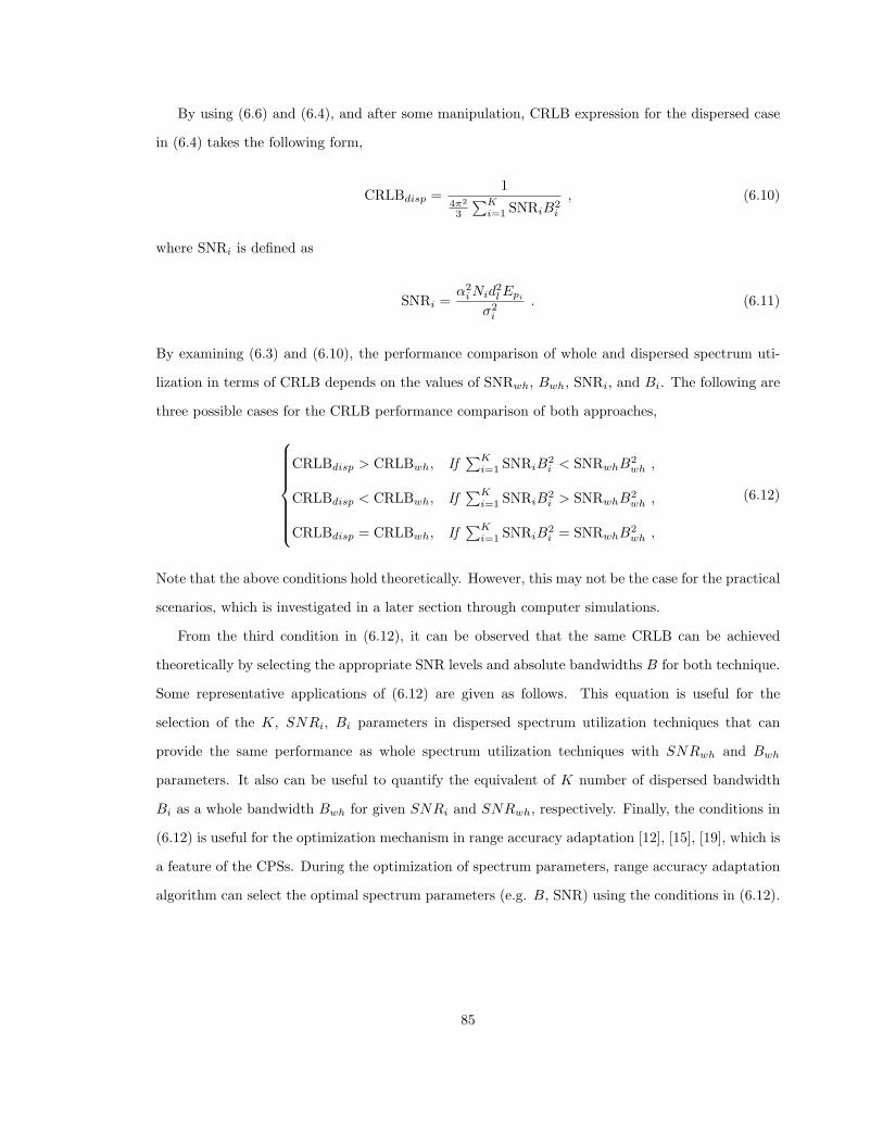
By using (6.6) and (6.4), and after some manipulation, CRLB expression for the dispersed case
in (6.4) takes the following form,
CRLBdisp =1
4π2
3
∑Ki=1 SNRiB2
i
, (6.10)
where SNRi is defined as
SNRi =α2
i Nid2l Epi
σ2i
. (6.11)
By examining (6.3) and (6.10), the performance comparison of whole and dispersed spectrum uti-
lization in terms of CRLB depends on the values of SNRwh, Bwh, SNRi, and Bi. The following are
three possible cases for the CRLB performance comparison of both approaches,
CRLBdisp > CRLBwh, If∑K
i=1 SNRiB2i < SNRwhB2
wh ,
CRLBdisp < CRLBwh, If∑K
i=1 SNRiB2i > SNRwhB2
wh ,
CRLBdisp = CRLBwh, If∑K
i=1 SNRiB2i = SNRwhB2
wh ,
(6.12)
Note that the above conditions hold theoretically. However, this may not be the case for the practical
scenarios, which is investigated in a later section through computer simulations.
From the third condition in (6.12), it can be observed that the same CRLB can be achieved
theoretically by selecting the appropriate SNR levels and absolute bandwidths B for both technique.
Some representative applications of (6.12) are given as follows. This equation is useful for the
selection of the K, SNRi, Bi parameters in dispersed spectrum utilization techniques that can
provide the same performance as whole spectrum utilization techniques with SNRwh and Bwh
parameters. It also can be useful to quantify the equivalent of K number of dispersed bandwidth
Bi as a whole bandwidth Bwh for given SNRi and SNRwh, respectively. Finally, the conditions in
(6.12) is useful for the optimization mechanism in range accuracy adaptation [12], [15], [19], which is
a feature of the CPSs. During the optimization of spectrum parameters, range accuracy adaptation
algorithm can select the optimal spectrum parameters (e.g. B, SNR) using the conditions in (6.12).
85

6.4 A Combining Technique for Dispersed Spectrum Utilization Systems
Combining signals received over dispersed bands at the receiver side is a crucial process and it
affects the performance of dispersed spectrum utilization systems. The signals at each branch can
be combined using different criterion. In this section, we propose an energy combining technique
based on maximizing total SNR criterion for dispersed spectrum utilization systems as shown in
Fig. 6.6. In this method, receive signal in each branch is correlated with the corresponding template
signal and the resultant signals are combined in such a way to maximize SNR. This is followed by
performing time delay estimation process.XTemplate 1r1(t)XTemplate 2r2(t)XTemplate KrK(t)
Time DelayEstimator...Figure 6.6 Energy combining technique for dispersed spectrum utilization systems.
6.5 Results and Discussions
In this section, performance of both exact and approximate CRLB is compared considering
whole spectrum utilization systems. This is followed by performance comparison of both whole and
dispersed spectrum utilization approaches for theoretical and practical cases.
86

The following simulation parameters are used for comparing the exact and approximate CRLB
and ML TOA estimator. For the pulse shape, Gaussian second order derivative is employed
p(t) = A
(1− 4πt2
ζ2
)e−2πt2/ζ2
, (6.13)
where A and ζ are parameters that are used to adjust the pulse energy and the pulse width, respec-
tively. A is selected in order to generate pulses with unit energy. For the given pulse shape, pulse
width is defined as Tp = 2.5ζ [19]. The signal bandwidth that is considered is 1MHz. Moreover,
uniformly distributed delay Ta = 5Tp is considered, i.e. U [0, Ta]. The number of training symbol
N that is considered is 1 and dl = [1]. The results are obtained over 3000 channel realizations with
channel fading coefficient α = 1 and are plotted in Fig. 6.7. According to the results, exact CRLB
performs better than approximate CRLB by approximately 3.7dB. This is due to the flat spectrum
assumption made during the derivation of B from β.
ML approach can be implemented by cross-correlating the received signal with template signal
and computing the minimum square error (MSE) of time delay estimates. The time delay estimates
are subject to ambiguity errors caused by the oscillatory nature of the signal correlation function [93].
The results in Fig. 6.7 as well as the results in the literature [93] indicates that MSE is a function of
SNR exhibiting threshold phenomenon. The SNR threshold for the results in Fig. 6.7 is 16dB and
it divides the SNR region into two distinct regimes [93], which are low and medium SNR regions.
Note that the SNR point where the transition from low to medium SNR regimes occurs is
referred as SNR threshold. MSE demonstrates a nonlinear behavior in the low SNR regime, whereas
this behavior becomes linear after the SNR threshold. This behavior is formulated by Barankin
bound [93]. An alternative definition of SNR threshold is developed from the results in Fig. 6.7,
which is the SNR point where the noise effects become negligible. As a result, bandwidth effects
also begin to contribute to the overall MSE performance. In other words, SNR is the dominant
parameter in the low SNR region and both SNR and B contributes to the overall MSE performance
after the SNR threshold. This definition is also useful to explain the performance gap between ML
and CRLB in the low SNR (or nonlinear) region. This is because of CRLB takes both SNR and B
(see (6.3)) into account during time delay estimate over the entire SNR region. Therefore, CRLB
performs better than ML in the low SNR region and it converges to approximate CRLB after the
87

SNR threshold. Moreover, ML performs better than approximate CRLB by 0.5dB according to the
results in Fig. 6.7.
0 5 10 15 20 25 3010
0
101
102
103
SNR [dB]
RM
SE
[m]
MLExact CRLBApprox. CRLB
Figure 6.7 Comparison of exact and approximate CRLB for whole spectrum utilization systems.
Performance of whole and dispersed spectrum utilization systems are compared considering ap-
proximate CRLB and ML TOA estimator. Performance comparison of both approaches are con-
ducted for three cases. The number of available dispersed bandwidth for all three cases is considered
to be 2, i.e. K = 2. In case 1, SNR1 + SNR2 = SNRwh, Bi = 1MHz and Bwh = 2MHz. For case
2, SNRi = SNRwh, Bi = Bwh = 2MHz. Finally, the parameters for case 3 are given as follows:
SNR1 + SNR2 = SNRwh, Bi = B = 2MHz. The remaining system parameters for all three cases
are common and they are given as follows. Training data dl = 1 is considered, where the number
of observation symbols for both whole and dispersed spectrum is 1, i.e. Ni = N = 1. In addition,
it is assumed that the spectral density of the noise is the same for the whole spectrum and all the
K branches of the dispersed spectrum techniques; i.e., σi = σ for i = 1, . . . , K. The Gaussian
second order derivative pulse shape is used. Therefore, the pulse shape for the whole and dispersed
spectrum methods are generated using Tp = 2.5ζwh, where ζwh = 1/2.5Bwh, and Tpi = 2.5ζi, where
ζi = 1/2.5Bi, respectively. For the practical cases, ML TOA estimator is employed. The combining
technique shown in Fig. 6.6 is used for dispersed spectrum utilization systems. Furthermore, the root
88

mean square error (RMSE) metric is considered to measure the performance of ML TOA estimator.
Note that all the results in this section are obtained over 10000 channel realizations.
For the theoretical case, (6.3) is denoted as CRLB-Whole and (6.10) is denoted as CRLB-
Dispersed. Similarly, ML TOA estimator for the whole and dispersed spectrum cases are denoted
as ML-Whole and ML-Dispersed, respectively. The results for case 1 are plotted in Fig. 6.8. CRLB-
Whole performs better than CRLB-Dispersed by 6dB for the entire SNR region. Since combined
total SNR for dispersed case is equal to SNRwh, this performance difference is due to B2wh = 4B2
i .
This result is justified by the first condition in (6.12). On the other hand, ML-Whole performs
similar to ML-Dispersed in the low SNR (nonlinear) region since combined total SNR for dispersed
case is equal to SNRwh. However, in the linear region (after the SNR threshold of 17dB), ML-
Whole and ML-Dispersed converges to CRLB-Whole and CRLB-Dispersed, respectively. In other
words, ML-Whole performs better than ML-Dispersed by 6dB in this region. Furthermore, the
SNR threshold for dispersed is less than the SNR threshold for whole case and this is due to noise
reduction obtained from combining process in the dispersed spectrum utilization case.
The results for case 2 are plotted in Fig. 6.9. According to the results, CRLB-Dispersed performs
better than CRLB-whole by 3dB for the entire SNR region. This is due to SNR gain obtained from
combining process in the dispersed case since Bi = B = 2MHz. This result is justified with the
second condition in (6.12). On the other hand, ML-Dispersed performs better than ML-Whole by
3dB in the low SNR region due to the SNR gain obtained from the combining process. The same
result is observed in the linear region since Bi = B. In other words, bandwidth does not cause any
performance difference.
In Fig. 6.10, the results for case 3 are shown. CRLB-Whole and CRLB-Dispersed performs same
for all the SNR values. This result is justified by the third condition in (6.12). Similarly, ML-Whole
and ML-Dispersed performs same over all SNR region since the combined SNR in dispersed case is
equal to SNRwh and Bi = B.
6.6 Conclusions
In this chapter, performance of whole and dispersed spectrum utilization approaches are com-
pared considering time delay estimation problem in cognitive positioning systems. A combining
technique based on maximizing SNR criterion is proposed for dispersed spectrum utilization sys-
tems. The CRLB for both approaches over AWGN channel are presented. Furthermore, performance
89
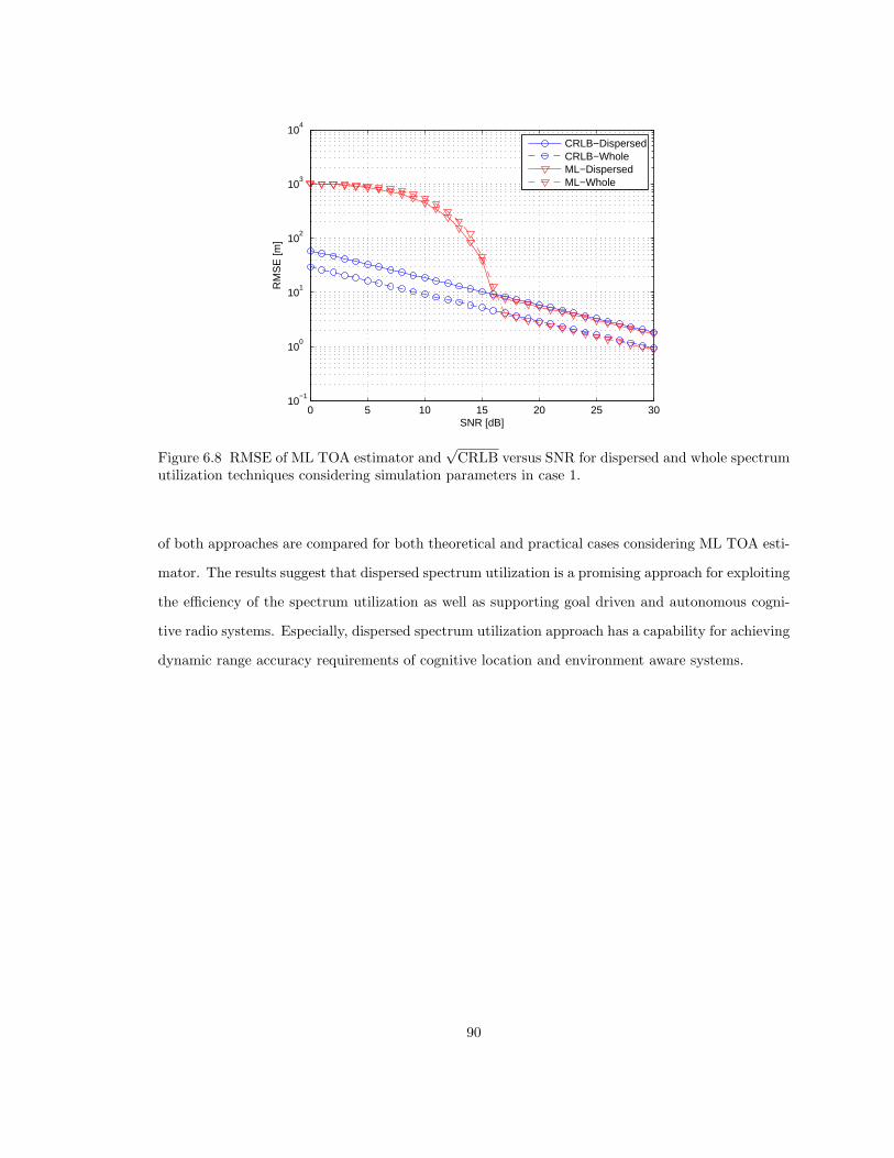
0 5 10 15 20 25 3010
−1
100
101
102
103
104
SNR [dB]
RM
SE
[m]
CRLB−DispersedCRLB−WholeML−DispersedML−Whole
Figure 6.8 RMSE of ML TOA estimator and√
CRLB versus SNR for dispersed and whole spectrumutilization techniques considering simulation parameters in case 1.
of both approaches are compared for both theoretical and practical cases considering ML TOA esti-
mator. The results suggest that dispersed spectrum utilization is a promising approach for exploiting
the efficiency of the spectrum utilization as well as supporting goal driven and autonomous cogni-
tive radio systems. Especially, dispersed spectrum utilization approach has a capability for achieving
dynamic range accuracy requirements of cognitive location and environment aware systems.
90

0 5 10 15 20 25 3010
−1
100
101
102
103
104
SNR [dB]
RM
SE
[m]
CRLB−DispersedCRLB−WholeML−DispersedML−Whole
Figure 6.9 RMSE of ML TOA estimator and√
CRLB versus SNR for dispersed and whole spectrumutilization techniques considering simulation parameters in case 2.
0 5 10 15 20 25 3010
−1
100
101
102
103
104
SNR [dB]
RM
SE
[m]
CRLB−DispersedCRLB−WholeML−DispersedML−Whole
Figure 6.10 RMSE of ML TOA estimator and√
CRLB versus SNR for dispersed and whole spectrumutilization techniques considering simulation parameters in case 3.
91

CHAPTER 7
LOCATION AWARE SYSTEMS IN COGNITIVE WIRELESS NETWORKS
7.1 Introduction
One of the most prominent features of cognitive radio (CR) technology is its location awareness.
Incorporation of this capability to CR brings challenges and opportunities such as location sensing,
seamless positioning and interoperability, statistical learning and tracking, security and privacy,
mobility management, adaptation of location aware systems, and location aware applications. Some
of these issues and applications have been studied for the legacy radios and wireless networks in some
extent. However, all of these issues need to be revisited in the CR and cognitive wireless network
(CWN) domains. Therefore, a location awareness engine handling all these issues and applications
in CWNs is proposed in Chapter 2. The focus of this chapter is to present some representative
applications of the location awareness engine that it can support.
Applications of the location awareness engine are folded under four major groups: location-based
services (e.g. monitoring real-time traffic), location-assisted network optimization (e.g. location-
assisted dynamic spectrum access systems), location-assisted transceiver optimization (e.g. location-
assisted link adaptation), and location-assisted environment identification (e.g. location-assisted
channel environment characterization). Only some representative applications of location-assisted
network optimization are presented in this chapter to demonstrate the utilization of location infor-
mation for different applications in CWNs.
In this chapter, a brief taxonomy of CWNs based on cognition, collaboration, and node diversity
criteria is presented. Implementation options of location awareness in cognitive radios and networks
are discussed. Furthermore, several location-assisted network optimization applications for CWNs
such as location-assisted dynamic spectrum access management, network planning and expansion,
and handover along with preliminary results are presented.
92

7.2 Cognitive Wireless Network Model
Cognition, collaboration, and node diversity are the main criteria that can be used to classify
CWNs. These networks consist of two major parts, which are central cognitive engine and nodes.
One can think of a central cognitive engine in CWNs like a mobile switching center with more
intelligence in cellular networks. We consider both CR base station and mobile station as a node in
this chapter.
Partitioning cognition features between the central cognitive engine of a network and cogni-
tive engine of nodes plays a key role to classify CWNs. In theory, various type of CWNs can be
developed between two extreme cognition limits, which are absolute centralized and distributed
(non-centralized) cognition [14]. In the former limit, central cognitive engine has full cognition ca-
pabilities whereas nodes possess limited cognition capabilities. Basically, central cognitive engine
can be considered as the brain and nodes are members. On the other hand, the structure is totally
opposite in the absolute distributed cognition case, where the full cognition capability is embedded
into the cognitive engine of each node. Note that this type of network will always have a central
cognitive engine to maintain network organization regardless of the cognition level of CR nodes.
Indeed, nodes will have more cognition capabilities as the technology advances. On the other hand,
ad-hoc CR network [94] can be considered as a network type between these two cognition limits.
CWNs can be classified under three types from the perspective of collaboration within a net-
work [95]. Collaboration can be between a node and central cognitive engine of network and/or
between nodes. Since there is a natural collaboration between central cognitive engine and nodes,
the following classification is based on the collaboration between nodes. The first type is so called
cooperative network, in which all the nodes agree on performing predefined (i.e. cooperative spec-
trum sensing) or ideally goal driven tasks collectively. Non-cooperative network is the second type
of network, in which there are no collaborations between nodes. On the other hand, if a group of
nodes do and the rest of them do not agree to collaborate, then this forms the third type of network
that is so called partially cooperative network. Ideally, CWNs can have a capability to transit from
one type to another dynamically depending on the collaboration of nodes. It is worth to note that
CR nodes and CWNs can have a capability to cooperate with the satellites such as in the case of
assisted-global positioning system (A-GPS).
93

Based on the node diversity criteria, CWNs can be grouped under two main categories: pure
cognitive wireless networks and mixed cognitive and non-cognitive wireless networks. As the names
imply, the former consists of only cognitive radio nodes and the latter composed of both cognitive
and non-cognitive radio nodes. Pure cognitive wireless networks can be divided further into two
subgroups, which are homogeneous and heterogeneous networks. For a given geographical area or
cell, all cognitive radio nodes are identical (they use same waveform) in the homogeneous networks.
For instance, a network consisting of only cognitive Worldwide Interoperability for Microwave Access
(WiMAX) nodes is an example for the homogeneous networks, which is illustrated in Fig. 7.1. On
the other hand, if the given geographical area or cell consists of mixture of different cognitive radio
nodes (i.e. WiMAX base stations, Ultrawideband (UWB) nodes), this type of network is called as
heterogeneous network [2]. In this type of network, a mobile device can roam across the cell borders
of the other networks and inter-operate with the other wireless devices. A representative example
of mixed cognitive and non-cognitive wireless networks is illustrated in Fig. 7.2. Notice that in this
type of networks interoperability is an issue. Although cognitive radios can communicate among
themselves and with non-cognitive radios, non-cognitive radio nodes may not be able to communicate
among themselves. Location information of mobile cognitive radio nodes play important roles to
achieve global mobility and seamless connectivity in CWNs. For instance, mobile cognitive radio
node can switch from WLAN to WiMAX networks as the user leaves home by tracking the location
of the user. Note that, in reality, the heterogeneity of CWNs can change dynamically as well.
7.3 Implementation Options
Learning through interactions of cognitive radio with the surrounding environment can be ac-
complished mainly in one of three ways: cooperative, self, and composite. Without loss of generality,
the details of each implementation option are provided in the context of location awareness in the
sequel.
In cooperative location awareness approach, (at least) two cognitive radios collaborate on learning
the distance between them by estimating the ranging information. In this approach, one of the
cognitive radios transmits signal (e.g. RF or acoustic) through channel environment and the other
cognitive radio extracts the ranging information from the received signal as illustrated in Fig. 7.3.
In other words, the transmitter and receiver are not co-located. Cooperative location awareness can
be accomplished by using cognitive positioning systems [12]. Both cognitive radios negotiate on the
94

CR1(WiMAX BS)CR2(WiMAX MS)
CR3(WiMAX MS)CR4(WiMAX MS)CR5(WiMAX MS) CR6(WiMAX MS)
Figure 7.1 Illustration of the homogeneous pure cognitive wireless networks; text in the parenthesesshow the instantaneous waveform of each cognitive radio node (CR: cognitive radio node).
ranging parameters that achieves given accuracy through cognitive ranging protocol illustrated in
Fig. 7.4. This protocol consists of three stages: ranging parameter setup, two-way TOA ranging,
time-stamp report. Both cognitive radios negotiate or provide feedbacks to each other during the
ranging parameter setup stage (loop). Once both agree on the parameters, the next two stages are
initiated. The last two stages are parts of conventional two-way TOA ranging protocol, which the
details of these steps can be found in [96].
Unlike to cooperative location awareness approach, self location awareness method enables a
cognitive radio to perform location awareness without the need of another cognitive radio or in-
frastructure. The self location awareness can be achieved in one of two ways, which are active and
passive manners as illustrated in Fig. 7.5. In active self location awareness methods, simply, both
transmitter and receiver are utilized and they are co-located. A perfect example for this approach in
the nature is bat echolocation system. Such system can be accomplished in cognitive radios by using
95

CR1(WiMAX BS)NCR2(WLAN Device)
CR3(WiMAX MS)CR2(CDMA MS)CR5(UWB Device) NCR4(GSM MS)
NCR1(TV Transmitter) CR4(CDMA BS)NCR3(Satellite)
NCR5(Bluetooth Device)Figure 7.2 Illustration of the mixed cognitive and non-cognitive wireless networks (NCR: non-cognitive radio nodes). EnvironmentCRDevice A CRDevice BRanging Parameter Setup LoopFigure 7.3 A conceptual model for cooperative location awareness between two cognitive radios.
cognitive radar [21] or cognitive sonar techniques. On the other hand, passive self location aware-
ness methods observe and acquire the signals (e.g. optic or acoustic) from the environment without
transmitting any signal. Basically, this approach requires only receptor such as image sensors. Hu-
man vision and hearing are two natural examples of passive self location awareness technique. Such
capabilities can be embodied into cognitive radios using aforementioned location sensing methods.
96

CR Device A CR Device BD1TtoaTpdTtoaTrt D2ACK1
ACK2D3ACK3
Ranging parameter setupTwo-way rangingTime-stamp report
Figure 7.4 Illustration of cognitive ranging protocol.Environmenta) Active b) Passive
EnvironmentFigure 7.5 A conceptual model for self location awareness: a) active, b) passive.
Both cooperative and self location awareness methods have some strengths and weaknesses.
For instance, cooperative methods have capability to provide absolute and relative ranging and
positioning information whereas the self techniques can provide only relative ranging information.
97

Furthermore, the implementation of closed-loop feedback (receiver-transmitter-environment) in self
location awareness architectures is less complex than that in cooperative location awareness archi-
tectures since the transmitter and receiver are co-located in the former architectures. Cognitive
radio can leverage the strengths of both cooperative and self location awareness methods, which is
referred as composite location awareness for supporting advanced and autonomous location aware
applications.
7.4 Location-based Services
Location-based services (LBSs) are well known location aware systems. By using the location
awareness capability of cognitive radios and networks, numerous location aware applications can be
developed. Therefore, some representative location aware applications are provided in Table 7.1.
Nevertheless, the focus of this chapter are location assisted network optimization methods, which
are discussed in the following sections.
7.5 Location-assisted Network Optimization
Various location-assisted network optimization algorithms can be developed for CWNs such as
location-assisted spectrum management, network plan and expansion, handover, dynamic channel
allocation, routing, power control, internetworking, and adaptive coverage system. However, only
the first three applications are discussed in this section.
7.5.1 Location-assisted Dynamic Spectrum Management
Under-utilization of the licensed bands and scarceness in the license-exempt bands prompt the
concept of efficient usage of spectrum. Basically, in the absence of the licensed users that have
the privileges to use their bands, unlicensed users can utilize these bands temporarily. This can be
achieved by using overlay and/or underlay spectrum access techniques. There are many different
proposals for dynamic spectrum management in CWNs. However, we consider three potential ap-
proaches proposed by the Federal Communications Commission (FCC) in the United States, which
are Listen-before-talk, Geolocation-database, and Local beacon techniques [97]. These schemes are
proposed for allowing unlicensed operations in the TV bands while preventing interference to TV
receptions. Moreover, a recently formed IEEE 802.22 working group for the Wireless Regional Area
Networks has the same vision as the FCC. The main goal of this group is to establish a CR-based
98

Table 7.1 Some representative location aware applications for cognitive radios and networks.
Application Type Applications
Location-based Services (LBS) • Public safety (e.g. police, fire),
• E911, E112,
• Package tracking,
• Child finder,
• Patient tracking,
• Real-time traffic services,
• Roadside assistance.
Location-assisted Network Optimization • Dynamic spectrum management,
• Network plan and upgrade,
• Handover,
• Dynamic channel allocation,
• Routing,
• Power management,
• Internetworking,
• Adaptive coverage system.
Location-assisted Transceiver Optimization • Adaptive beamforming
• Interference avoidance,
• Link adaptation,
Location-assisted Environment Identification • Channel environment characterization,
• LOS/NLOS identification.
standard that allows unlicensed users to utilize the bands allocated to TV broadcast services in a
non-interfering fashion. It is worth to mention that low frequency analog TV bands (54− 862MHz)
has some attractive features for wireless broadband services such as achieving long-distance trans-
99

mission. Since the Geolocation-Database and Local Beacon techniques utilize location information,
the other technique is out of scope of this section.
According to Geolocation-database approach, licensed users (e.g. TV transmitter) are equipped
with the location sensing device to estimate their current location information. The licensed users
provide their spectrum and location information to the FCC central database. The FCC database
broadcasts available channel information along with the location information of the licensed users.
On the other hand, unlicensed users are also equipped with the location sensing device to estimate
their current locations. Unlicensed users cross-check their locations with the location of licensed
users in order to obtain the channel information that they can use locally. Two major concerns
regarding this scheme are the reliability of the current geolocation technologies and the performance
of FCC central database. For instance, some TV broadcasters point out that the GPS does not
provide reliable location information of a user that is located in indoor environments. However,
some deficiencies of GPS such as low accuracy and indoor inoperability are addressed with the
recent advances in this technology such as A-GPS and Indoor GPS. Alternatively, the licensed users
and unlicensed users can utilize more reliable positioning techniques such as the CPSs to obtain
their current location information. The other concern is that the current FCC central databases are
slow to catch up the frequency changes and they are not 100 % reliable. This is a valid concern and
the FCC is aware of this issue. As a solution, the FCC can upgrade its database technology in order
to be used for the spectrum sensing and allocation purposes.
Local beacon method is pretty similar to geolocation-database scheme except that the database
will be placed in a local cell to manage the spectrum. Cognitive base station within a cell broadcasts
local geolocation-database at predefined time intervals. A snapshot of local geolocation-database
example is illustrated in Table 7.2. Unlicensed CR nodes within local cell receive the geolocation-
database and cross-check with their own location information. Consequently, they can determine
their prospective spectrum plans (e.g. center frequency and absolute bandwidth). In the US, the
FCC states that short-range signals will be used to broadcast the available channel information.
Since the FCC does not specify the ”short-range signals” term, long-range signals can be used and
they can introduce interferences to the neighbor cells. Consequently, such signals can degrade the
performance of this scheme significantly and even it can shut down the system. Although these
two location-assisted dynamic spectrum management approaches are recommended, there are many
challenges to implement them, which are open research areas.
100
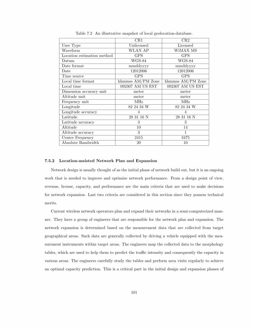
Table 7.2 An illustrative snapshot of local geolocation-database.
CR1 CR2User Type Unlicensed LicensedWaveform WLAN AP WiMAX MSLocation estimation method GPS GPSDatum WGS-84 WGS-84Date format mmddyyyy mmddyyyyDate 12012006 12012006Time source GPS GPSLocal time format hhmmss AM/PM Zone hhmmss AM/PM ZoneLocal time 092307 AM US EST 092307 AM US ESTDimension accuracy unit meter meterAltitude unit meter meterFrequency unit MHz MHzLongitude 82 24 34 W 82 24 34 WLongitude accuracy 4 4Latitude 28 31 16 N 28 31 16 NLatitude accuracy 3 3Altitude 10 14Altitude accuracy 3 1Center Frequency 2415 3475Absolute Bandwidth 20 10
7.5.2 Location-assisted Network Plan and Expansion
Network design is usually thought of as the initial phase of network build out, but it is an ongoing
work that is needed to improve and optimize network performance. From a design point of view,
revenue, license, capacity, and performance are the main criteria that are used to make decisions
for network expansion. Last two criteria are considered in this section since they possess technical
merits.
Current wireless network operators plan and expand their networks in a semi-computerized man-
ner. They have a group of engineers that are responsible for the network plan and expansion. The
network expansion is determined based on the measurement data that are collected from target
geographical areas. Such data are generally collected by driving a vehicle equipped with the mea-
surement instruments within target areas. The engineers map the collected data to the morphology
tables, which are used to help them to predict the traffic intensity and consequently the capacity in
various areas. The engineers carefully study the tables and perform area visits regularly to achieve
an optimal capacity prediction. This is a critical part in the initial design and expansion phases of
101
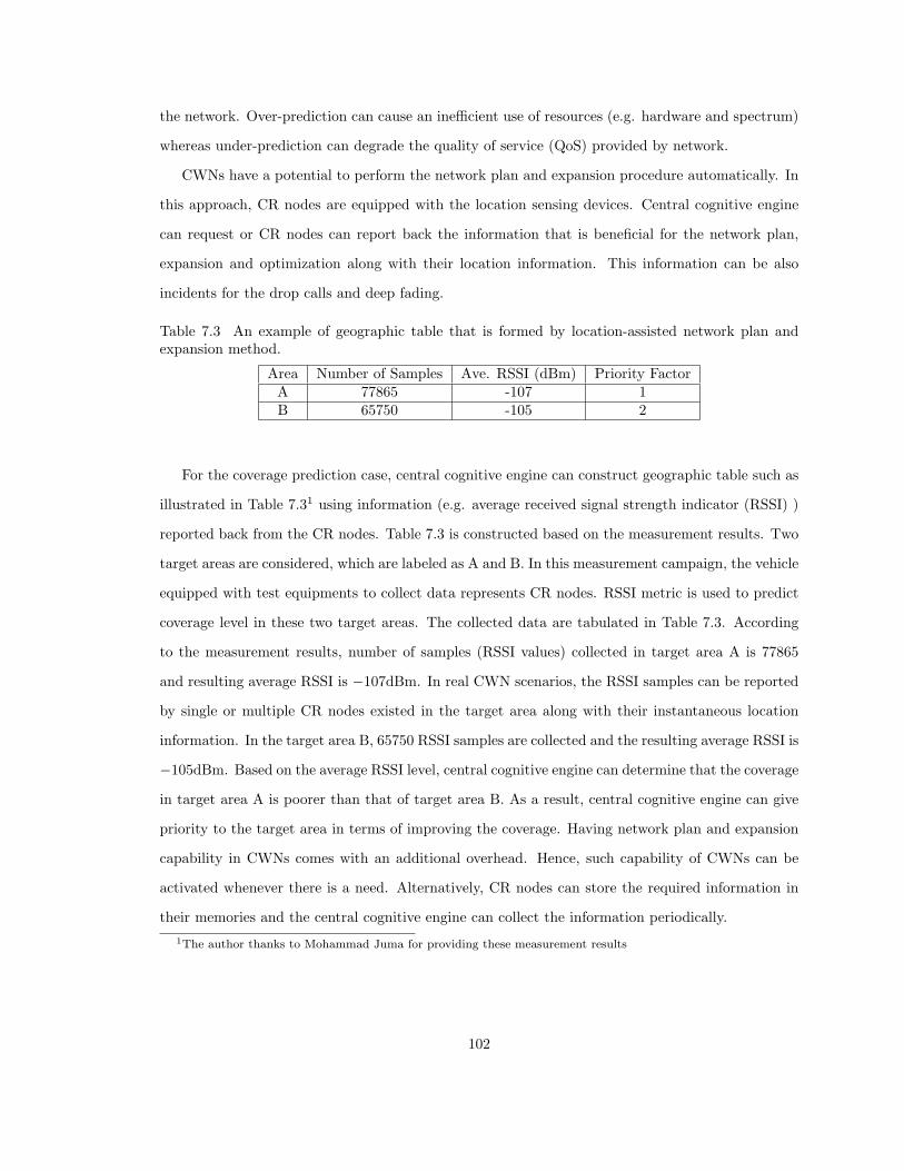
the network. Over-prediction can cause an inefficient use of resources (e.g. hardware and spectrum)
whereas under-prediction can degrade the quality of service (QoS) provided by network.
CWNs have a potential to perform the network plan and expansion procedure automatically. In
this approach, CR nodes are equipped with the location sensing devices. Central cognitive engine
can request or CR nodes can report back the information that is beneficial for the network plan,
expansion and optimization along with their location information. This information can be also
incidents for the drop calls and deep fading.
Table 7.3 An example of geographic table that is formed by location-assisted network plan andexpansion method.
Area Number of Samples Ave. RSSI (dBm) Priority FactorA 77865 -107 1B 65750 -105 2
For the coverage prediction case, central cognitive engine can construct geographic table such as
illustrated in Table 7.31 using information (e.g. average received signal strength indicator (RSSI) )
reported back from the CR nodes. Table 7.3 is constructed based on the measurement results. Two
target areas are considered, which are labeled as A and B. In this measurement campaign, the vehicle
equipped with test equipments to collect data represents CR nodes. RSSI metric is used to predict
coverage level in these two target areas. The collected data are tabulated in Table 7.3. According
to the measurement results, number of samples (RSSI values) collected in target area A is 77865
and resulting average RSSI is −107dBm. In real CWN scenarios, the RSSI samples can be reported
by single or multiple CR nodes existed in the target area along with their instantaneous location
information. In the target area B, 65750 RSSI samples are collected and the resulting average RSSI is
−105dBm. Based on the average RSSI level, central cognitive engine can determine that the coverage
in target area A is poorer than that of target area B. As a result, central cognitive engine can give
priority to the target area in terms of improving the coverage. Having network plan and expansion
capability in CWNs comes with an additional overhead. Hence, such capability of CWNs can be
activated whenever there is a need. Alternatively, CR nodes can store the required information in
their memories and the central cognitive engine can collect the information periodically.1The author thanks to Mohammad Juma for providing these measurement results
102

7.5.3 Location-assisted Handover
Handover is an important mechanism in CWNs likewise in legacy cellular networks. In [98],
a location-based handover algorithm is proposed for the GSM networks and the performance of
conventional handover and the proposed handover algorithms are compared. The measurement
results show that the location-based handover algorithm provides 30 % reduction in the number
of handovers compare to the conventional RSSI-based handover for a given call. In this section, a
set of measurement results (without detailed performance analysis) are presented to demonstrate
the impact of handover mechanism on the network performance. Furthermore, a location-assisted
handover mechanism is proposed for CWNs to reduce number of handovers and consequently network
load.
The majority of the current handover mechanisms are based on only signal strength, signal
quality and cell traffic parameters due to the complexity limitations. As the QoS requirements
increase, the current handover algorithms such as RSSI-based handover start to lag. Therefore,
they can be replaced with more efficient handover algorithms such as location-assisted handover
method, which is based on use of the location information of mobile stations. In this algorithm, the
handover zones in which all mobile stations are served by the predetermined candidates are defined.
Mobile stations are equipped with the location sensing devices to report their locations back to
mobile switching center. Once a mobile station enters into a handover zone, mobile station can be
served by one of the predetermined candidates. Moreover, these candidates can be prioritized in the
case of congestion, site outages or exceptions. The location-assisted handover algorithm can reduce
the number of handovers along the intended road, release the signaling load on the network, and
maintain the handover pattern between the serving sites in other areas.
A measurement campaign is conducted in a live cellular network to obtain the performance
of RSSI-based handover and location-assisted handover in the presence of ping pong effects. The
experiment is performed as follows: the first drive test is performed to obtain the performance of
RSSI-based handover and it is conducted between two cells to capture the handover pattern along
one stretch (5 miles) of a highway. The signal strength, signal quality, and handover pattern of the
test phone (MS2) in the dedicated mode are shown in Fig. 7.6a and 7.6b, and 7.6c2, respectively.
The dedicated mode is the mode of the test phone when a call is in progress. During this trial, the2The author thanks to Mohammad Juma for providing these measurement results
103

phone is allowed to handover from cell 200C to cell 201B. It is clear from the results that neither
RSSI nor the signal quality is affected from the handover process.
Figure 7.6 Test phone (MS2) in the dedicated mode: a) signal quality, b) signal strength, c) handoverpattern.
In the second part of the experiment, the performance of location-assisted handover algorithm
is observed. Since the test phone does not have the location estimation capability, the performance
of location-assisted handover mechanism is obtained using a priori location information. Basically,
we have the information about the boundaries of actual cell, in which the part of the highway that
is used during the experiment resides. This a priori information is used to eliminate the need for
the location sensing device. As a result, the test phone (MS1) is locked to the actual cell prior to
104

driving the test vehicle in the opposite direction of the same part of highway. The test phone is
set to not accept any handover offer from any cells in the surrounding areas. The signal strength
and signal quality profiles of the test phone are measured and the results are shown in Fig. 7.7a
and 7.7b3, respectively. It is observed that the drop call does not occur and the signal quality as
well as the signal strength are preserved in the handover region as shown in Fig. 7.7. In the case
of RSSI-based handover, the handover decision is initiated too early, which resulted in excessive
number of handovers. Although the handover did not occur during the location-assisted handover
experiment due to the restriction that we set in the test phone, the handover occurrence is inevitable
in reality for this case. In such case, the proposed range accuracy adaptation can be utilized to reduce
number of handovers. This can be accomplished to improve range accuracy adaptively in handover
zone. In summary, we can conclude that the number of handovers can be reduced significantly by
employing the location-assisted handover algorithms along with range accuracy adaptation method.
As a result, it is recommended to incorporate the location-assisted handover algorithms into CWNs
to optimize handover mechanism.
Figure 7.7 Test phone (MS1) in the locked mode: a) signal quality, b) signal strength.
3The author thanks to Mohammad Juma for providing these measurement results
105

7.6 Conclusions
A classification of cognitive wireless networks based on the cognition, collaboration, and node
diversity criteria is provided. Implementation options and challenges for the location awareness in
cognitive radios and networks are discussed. Several representative examples of location-assisted
network optimization are discussed to demonstrate applications of location awareness in cognitive
radios. The preliminary results show that location information plays an important role in network
optimization and we strongly recommend to balance the utilization of location information in the
cognitive wireless networks and the protection of user privacy. Detailed performance analysis of the
location-assisted optimization algorithms can be investigated further.
106

CHAPTER 8
CONCLUSIONS AND FUTURE WORKS
In this dissertation, we investigated the following topics: development of conceptual model for
cognitive radio with location and environment awareness engines, cognitive positioning systems along
with range accuracy adaptation, time delay estimation for whole spectrum utilization considering
practical challenges, dispersed spectrum utilization method and its performance for time delay esti-
mation problem, comparison of whole and dispersed spectrum utilization approaches in the context
of time delay estimation, and some representative location aware systems in cognitive wireless net-
works. In what follows, the summary of the contributions are presented. Then, potential directions
of our future work are provided.
In Chapter 2, a cognitive radio architecture with location and environment awareness engines
and cycles is developed in order to support goal driven, autonomous, and advanced location aware
systems. The architecture consists of engines (cognitive, location awareness, environment awareness,
and spectrum awareness engines), adaptive waveform generation/processing, and sensing interface
(radiosensing, radiovision, radiohearing sensors). The functionalities of location and environment
awareness engines are identified and presented with details. Finally, the details of radiovision,
radiohearing, and radiosensing sensors are presented.
In Chapter 3, cognitive positioning systems (CPS) for the location awareness engine is developed.
One of the main features of the CPS is range accuracy adaptation, which is developed by inspiring
from the range adaptation behavior of bats. Therefore, ML range accuracy adaptation algorithm is
proposed to achieve arbitrarily given range accuracy requirements. The proposed ML range accuracy
adaptation employs CRLB information at the transmitter side to optimize transmission parameters
for the given range accuracy requirements and ML location estimator in the receiver side. Therefore,
CRLBs for both AWGN and multipath channels are derived. The performance of ML range accuracy
adaptation is simulated in dynamic spectrum access environment and compared to the theoretical
bound. The results show that there is a margin between the practically achieved and desired range
107

accuracy. Therefore, three potential approaches are introduced in order to improve the performance
of the proposed method (i.e. reducing the margin). These approaches are hybrid overlay and un-
derlay dynamic spectrum access systems (HDSASs), dispersed spectrum utilization, and employing
suboptimal lower bounds such as Ziv-Zakai lower bound (ZZLB) for the parameter optimization. In
this chapter, we only emphasize on the HDSASs. In addition, a switching mechanism that manages
the transition between overlay and underlay dynamic spectrum access schemes for the HDSASs is
proposed.
In Chapter 4, we investigate the performance of time delay estimation using whole spectrum
utilization approach in dynamic spectrum access systems. Therefore, asymptotic frequency domain
CRB is derived through Whittle formula. The effects of dynamic spectrum access systems, especially
bandwidth and carrier frequency, on the performance of time delay estimator are investigated. In
addition, the effects of different channel environment on the performance of time delay estimator
considering frequency dependence feature of channel environment as metric are studied. Further-
more, for the practical considerations, a generic list of TOA ranging related channel statistics are
identified and quantified through computer simulations.
In Chapter 5, a new method for exploiting the spectrum utilization that is referred dispersed
spectrum utilization is introduced. A cognitive radio transceiver for this new method is developed.
The performance of this transceiver is studied in the context of time delay estimation. Hence, a
generic CRLB is derived considering unknown channel coefficients and carrier frequency offsets.
Then, the effects of various modulation and unknown channel coefficients and carrier frequency
offsets on the accuracy of time delay estimation are quantified. Finally, numerical results are obtained
to verify the theoretical analysis.
In Chapter 6, the performance of whole and dispersed spectrum utilization approaches are com-
pared in the context of time delay estimation for theoretical and practical scenarios. Hence, cognitive
radio transceivers for both approaches are proposed. A combining technique based on maximizing
signal to noise ratio (SNR) criterion is proposed for the dispersed spectrum utilization approach.
Consequently, CRLBs for both approaches are presented as well considering AWGN channel. For
the practical considerations, ML TOA estimator is considered. Finally, the performance of both ap-
proaches are compared by providing theoretical (i.e. CRLBs) and practical (i.e. ML TOA estimator)
results.
108

In Chapter 7, a taxonomy for cognitive wireless network is presented. This is followed by the
discussion of implementation options challenges of cognitive radios and networks. Then, several
potential cognitive location aware systems are presented with preliminary results in order to demon-
strate the utilization of location information in cognitive radios and networks. These systems are
categorized under four group:
• Location-based services (LBS),
• Location-assisted network optimization,
• Location-assisted transceiver optimization,
• Location-assisted environment identification.
For each group, various potential cognitive location aware applications are listed and some repre-
sentative location-assisted network optimization applications with preliminary results are presented.
Note that development of each of these systems can be considered as future work.
After providing the specific contributions of this dissertation, we summarize some of the directions
of our future work in the sequel.
Each functionality of the proposed cognitive radio architecture with location and environment
awareness engines is an open research area. Especially, the functionalities of location awareness
engine, which are given as follows, are active research areas:
• Sensing interface (radiosensing, radiovision, radiohearing),
• Location sensing and adaptation (focus of this dissertation, still there are many open issues,
which will be presented later in this section),
• statistical learning and tracking,
• Seamless positioning and interoperability,
• Mobility management,
• Secure positioning systems and privacy protection methods,
• Location aware systems.
109

During the development of this dissertation, we discovered several fundamental problems for the
realization cognitive radio, which are presented as follows.
Since the available spectrum in cognitive radios is dynamic, statistical modeling of dynamic
spectrum utilization for a given geographical region is a must in order to evaluate the performance
of cognitive radio algorithms. This is a crucial and open issue in cognitive radio literature.
The propagation channel is the bottleneck of wireless systems. The observed channel at the
wireless receiver mainly depends on the transmission parameters and the surrounding environment.
Hence, the first task for developing a wireless system (i.e., transceiver) for a given environment and
transmission parameters is to statistically model the propagation characteristics of the environment.
A wireless channel is generally described by two main sets of statistics: large statistics and small
statistics. The large and small statistics of the given channel environment are conventionally obtained
by conducting channel measurement campaigns. However, in cognitive wireless systems, transmission
parameters are dynamic due to the dynamic available spectrum and the goal driven autonomous
operation feature of cognitive radios. Since the transmission parameters such as bandwidth, carrier
frequency, transmit power are dynamic in cognitive systems, the observed channel and corresponding
statistics are also dynamic. It is a challenging task to realize and design cognitive wireless systems
for such dynamic channel environments. As a result, there is a need to develop rapid and low
complexity channel statistics acquisition methods.
Two potential approaches for channel statistics acquisition in cognitive wireless networks are
off-line and on-line channel statistics acquisition. In the first approach, the channel statistics are
obtained from the cognitive base station for the given geographical area [24]. In this approach,
it is assumed that cognitive radios have their position information. A cognitive radio provides its
transmission parameters and position information to the cognitive base station in order to obtain
the channel statistics information for its position. Then, the cognitive base station retrieves the
channel statistics for the given position from a pre-built database by mapping the position to the
corresponding channel statistics information [24]. The second approach, which is the on-line method,
is based on the idea of acquiring channel statistics information between two cognitive radios in real-
time (i.e., a cognitive base station and a cognitive radio node). It is obvious that this is a challenging
task to achieve. As a result, development of rapid and low complexity channel statistics acquisition
methods is a current research topic.
110

Since the utilized spectrum, transmission parameter, cognitive radio channel are dynamic, the
cognitive radio receiver is dynamic as well. Therefore, development of dynamic, low complexity, and
rapid cognitive radio receivers that can cope with dynamic spectrum utilization, transmission and
channel conditions is an active research area.
The proposed CPS, range accuracy adaptation, whole and dispersed utilization methods are
mainly studied for theoretical cases for proofing the concepts. In this dissertation, the CPS and
range accuracy adaptation method are developed using time of arrival statistics. However, the
analysis can be extended for the case of RSSI and AOA statistics. Furthermore, range estimation
between two cognitive radios (i.e. 1-D location information) is considered. The current study can
be extended to the estimation of 2-D and 3-D location information. In addition, CRLB, which is
the optimal bound, is utilized for the parameter optimization in the range accuracy adaptation.
More practical (or suboptimal) bounds such as ZZLB and Barankin bound can be considered for
the parameter optimization and this can be investigated further.
In addition, a large number of research challenges and problems are identified by introducing the
method of dispersed spectrum utilization. For instance, development of signaling, transmitter archi-
tectures and algorithms, channel behaviors, receiver structures and algorithms, and signal processing
techniques for the dispersed spectrum utilization systems are open research areas. More specifically,
we studied performance of dispersed spectrum utilization systems considering AWGN channel in or-
der to proof the concept and explore the fundamental challenges. Therefore, the present study can
be extended to the multipath channel case. In addition, we study the effects of carrier frequency off-
set (CFO) on the performance of the dispersed spectrum utilization systems in this study. However,
additional practical impairments such as out-of-band radiation for each band can be included to the
analysis. Furthermore, performance and complexity of the dispersed spectrum utilization systems
for different waveforms such as OFDM, UWB [99], and CDMA can be investigated and compared.
Finally, different combining technique can be developed for dispersed spectrum utilization systems.
111

REFERENCES
[1] “Human Consciousness,” 2007. [Online]. Available: www.iddl.vt.edu/
[2] H. Celebi and H. Arslan, “Utilization of Location Information in Cognitive Wireless Net-works,” IEEE Wireless Communications Magazine-Special issue on Cognitive Wireless Net-works, vol. 14, no. 4, pp. 6–13, Aug. 2007.
[3] Y. Xing, R. Chandramouli, and S. Mangold, “Dynamic Spectrum Access in Open SpectrumWireless Networks,” IEEE J. Selec. Commun., vol. 24, no. 3, pp. 626–637, March 2006.
[4] N. Sai Shankar, C. Cordeiro, and K. Challapali, “Spectrum Agile Radios: Utilization andSensing Architectures,” in First IEEE International Symposium on New Frontiers in DynamicSpectrum Access Networks, Baltimore, MD, USA, Nov. 2005, pp. 160–169.
[5] H. Arslan and M. E. Sahin, “Cognitive UWB-OFDM: Pushing Ultrawideband Beyond Its Limitvia Opportunistic Spectrum Usage,” Journal of Communications and Networks-Special Issueon Spectrum Resource Optimization, vol. 8, no. 2, pp. 151–157, June 2006.
[6] R. A. Altes, “A Theory for Animal Echolocation and Its Application to Ultrasonics,” in IEEEUltrasonics Symposium, Moneterey, California, USA, Nov. 1973, pp. 67–72.
[7] T. K. Horiuchi, “Seeing in the dark: neuromorphic vlsi modeling of bat echolocation,” IEEESignal Processing Mag., vol. 22, no. 5, pp. 134–139, August 2005.
[8] D. Bank and T. Kampke, “High-Resolution Ultrasonic Environment Imaging,” vol. 23, no. 2,pp. 370–381, April 2007.
[9] H. Arslan, Cognitive Radio, Software Defined Radio, and Adaptive Wireless Systems. Springer,June 2007.
[10] J. Mitola and G. Q. Maguire, “Cognitive radio: Making software radios more personal,” IEEEPersonal Commun. Mag., vol. 6, no. 4, pp. 13–18, August 1999.
[11] “IEEE 1900 Standards Committee on Next Generation Radio and Spectrum Management,”2006. [Online]. Available: http://www.ieeep1900.org/
[12] H. Celebi and H. Arslan, “Cognitive Positioning Systems,” IEEE Trans. Wireless Commun.,vol. 6, no. 12, pp. 4475–4483, Dec. 2007.
[13] J. O. Neel, “Analysis and design of cognitive radio networks and distributed radio resource man-agement algorithms,” Ph.D. dissertation, Virginia Polytechnic Institute and State University,VA, Sept. 2006.
[14] S. Haykin, “Cognitive Radio: Brain-empowered Wireless Communications,” IEEE J. Select.Areas Commun., vol. 23, no. 2, pp. 201–220, Feb. 2005.
[15] H. Celebi and H. Arslan, “Enabling location and environment awareness in cognitive radios,”Elsevier Computer Communications-Special Issue on Advanced Location-Based Services, vol. 31,no. 6, pp. 1114–1125, April 2008.
112

[16] H. Celebi, H. Arslan, “Adaptive Positioning Systems for Cognitive Radios,” in IEEE Symposiumon New Frontiers in Dynamic Spectrum Access Networks (DySpan), Dublin, Ireland, Apr. 2007,pp. 78–84.
[17] H. Celebi and H. Arslan, “Ranging Accuracy in Dynamic Spectrum Access Networks,” IEEECommun. Lett., vol. 11, no. 5, pp. 405–407, May 2007.
[18] H. Celebi, I. Guvenc, and H. Arslan, “On the statistics of channel models for uwb ranging,” inProc. IEEE Sarnoff Symposium, Princeton, NJ, March 2006, to appear.
[19] S. Gezici, H. Celebi, H. V. Poor, and H. Arslan, “Fundamental limits on time delay estimationin dispersed spectrum cognitive radio systems,” IEEE Trans. on Wireless Communications,June 2008, under revision.
[20] S. Haykin, “Cognitive radio: Brain-empowered wireless communications,” IEEE J. Select AreasCommun., vol. 23, no. 2, pp. 201–220, Feb. 2005.
[21] ——, “Cognitive radar: a way of the future,” IEEE Signal Processing Mag., vol. 23, no. 1, pp.30–40, Jan. 2006.
[22] Y. Zhao, J. H. Reed, S. Mao, and K. K. Bae, “Overhead analysis for radio environment mapen-abled cognitive radio networks,” in Proc. IEEE Workshop on Networking Technologies for Soft-ware Defined Radio Networks, Reston, VA, Sep. 2006, pp. 18–25.
[23] I. Akyildiz, W. Lee, M. Vuran, and S. Mohanty, “Next generation/dynamic spectrum ac-cess/cognitive radio wireless networks: A survey,” Elsevier Computer Networks, vol. 50, no. 13,pp. 2127–2159, 2006.
[24] H. Arslan and S. Yarkan, “Exploiting Location Awareness Towards Improved Wireless SystemDesign in Cognitive Radio,” IEEE Communications Magazine, 2007, to appear.
[25] D. Cabric, S. M. Mishra, and R. W. Brodersen, “Implementation issues in spectrum sensingfor cognitive radios,” in IEEE Thirty-Eighth Asilomar Conference on Signals, Systems andComputers, Pacific Grove, California, USA, Nov. 2004, pp. 772–776.
[26] H.-H. Nagel, “Steps Towards a Cognitive Vision System,” Artificial Intelligence Magazine,vol. 25, no. 2, pp. 31–50, 2004.
[27] R. Koch, “Dynamic 3-D scene analysis through synthesis feedback control,” IEEE Trans. onPattern Analysis and Machine Intelligence, vol. 15, no. 6, pp. 556–568, June 1993.
[28] Y.-H. Lu and E. J. Delp, “Image-based location awareness and navigation: who cares?” inIEEE Southwest Symposium on Image Analysis and Interpretation, Lake Tahoe, Nevada, USA,March 2004, pp. 26–30.
[29] P. Luley, A. Almer, C. Seifert, G. Fritz, and L. Paletta, “A Multi-Sensor System for MobileServices with Vision Enhanced Object and Location Awareness,” in IEEE International MobileCommerce and Services, Munich, Germany, July 2005, pp. 52–59.
[30] T. Starner, B. Schiele, and A. Pentland, “Visual context awareness via wearable computing,”in IEEE International Symposium on Wearable Computers, Pittsburgh, PA, USA, Oct. 1998,pp. 50–57.
[31] A. Quazi, “An overview on the time delay estimate in active and passive systems for targetlocalization,” IEEE Trans. Acoust., Speech, Signal Processing, vol. 29, no. 3, pp. 527–533, 1981.
113

[32] A. Smith, H. Balakrishnan, M. Goraczko, and N. B. Priyantha, “Tracking Moving Devices withthe Cricket Location System,” in 2nd International Conference on Mobile Systems, Applicationsand Services, Boston, MA , USA, June 2004.
[33] J. Agre, A. Akinyemi, L. Ji, R. Masuoka, and P. Thakkar, “A layered architecture for location-based services in wireless ad hoc networks,” in Proc. IEEE Aerospace Conference, vol. 3, BigSky, MT, USA, March 2002, pp. 1085–1097.
[34] N. Patwari, A. Hero, M. Perkins, N. Correal, and R. O’Dea, “Relative location estimation inwireless sensor networks,” IEEE Trans. on Signal Processing, vol. 51, no. 8, pp. 2137–2148,Aug. 2003.
[35] “Standard Molodensky Datum Conversion,” 2006. [Online]. Available:http://www.colorado.edu/geography/
[36] G. Sun, J. Chen, W. Guo, and K. Liu, “Signal processing techniques in network-aided posi-tioning: a survey of state-of-the-art positioning designs,” IEEE Signal Processing Mag., vol. 22,no. 4, pp. 12–23, july 2005.
[37] S. Feng and W. Y. Ochieng, “User Level Autonomous Integrity Monitoring for Seamless Po-sitioning in All Conditions and Environments,” in Proceedings of The European NavigationConference, Manchester, UK, May 2006.
[38] X. Li, “RSS-Based Location Estimation with Unknown Pathloss Model,” IEEE Trans. WirelessCommun., vol. 5, no. 12, pp. 3626–3633, Dec. 2006.
[39] “IEEE Standard Computer Dictionary: A Compilation of IEEE Standard ComputerGlossaries,” New York, NY, 1990. [Online]. Available: http://www.ieeexplore.ieee.org
[40] S. Capkun and J. Hubaux, “Secure positioning in wireless networks,” IEEE J. Select. AreasCommun., vol. 24, no. 2, pp. 221–232, Feb. 2006.
[41] “Geographic Location/Privacy (geopriv),” 2006. [Online]. Available: http://www.ietf.org/
[42] M. Brunato and R. Battiti, “Statistical learning theory for location fingerprinting in wirelessLANs,” Elsevier Computer Networks, vol. 47, no. 6, pp. 825–845, 2005.
[43] A. F. Molisch, “Ultrawideband Propagation Channels-Theory, Measurement, and Modeling,”IEEE Trans. Veh. Technol., vol. 54, no. 5, pp. 1528–1545, Sept. 2005.
[44] C. Sinka and J. Bito, “Rain attenuation countermeasure technique for broadband fixed wirelessaccess networks,” in Twelfth International Conference on Antennas and Propagation, vol. 1,UK, March 2003, pp. 441–444.
[45] M. Vossiek, L. Wiebking, P. Gulden, J. Wieghardt, C. Hoffmann, P. Heide, S. Technol, andG. Munich, “Wireless Local Positioning,” IEEE Microwave Magazine, vol. 4, no. 4, pp. 77–86,2003.
[46] “Federal Communications Commission (FCC) 911 Services,” 2006. [Online]. Available:http://www.fcc.gov/911/enhanced/
[47] “StarFire: A Global High Accuracy Differential GPS System,” 2006. [Online]. Available:http://www.navcomtech.com
[48] “A Taxonomy of Indoor and Outdoor Positioning Techniques for Mobile Location Services,”2003. [Online]. Available: www.acm.org
114

[49] F. van Diggelen, “Indoor GPS theory & implementation,” in IEEE Position, Location andNavigation Symposium, Palm Springs, CA, USA, April 2002, pp. 240–247.
[50] “Geolocation Development Document,” 2006. [Online]. Available: http://www.ieee802.org/22/
[51] C. Fretzagias and M. Papadopouli, “Cooperative Location-Sensing for Wireless Networks,” inProc. IEEE Pervasive Computing and Communications, Orlando, FL, March 2004, pp. 121–131.
[52] Y. Qi and H. Kobayashi, “On Relation among Time Delay and Signal Strength based Geolo-cation Methods,” in Proc. IEEE Globecom Conf., vol. 7, San Francisco, CA, Dec 2003, pp.4079–4083.
[53] B. Fette, Cognitive Radio Technology. Newnes, 2006.
[54] S. Gezici, Z. Tian, G. B. Giannakis, H. Kobayashi, A. F. Molisch, H. V. Poor, and Z. Sahinoglu,“Localization via UWB Radios,” IEEE Signal Processing Mag., vol. 22, no. 4, pp. 70–84, July2005.
[55] J. Hightower and G. Borriello, “A Survey and Taxonomy of Location Systems for UbiquitousComputing,” University of Washington, Tech. Rep., 2001.
[56] H. V. Poor, An Introduction to Signal Detection and Estimation. New York: Springer-Verlag,1994.
[57] Y. Qi, “Analysis of wireless geolocation in a non-line-of-sight environment,” Ph.D. dissertation,Princeton University, New Jersey, Nov. 2003.
[58] Y. Qi, H. Kobayashi, and H. Suda, “Analysis of wireless geolocation in a non-line-of-sightenvironment,” IEEE Trans. Wireless Commun., vol. 5, no. 3, pp. 672–681, march 2006.
[59] B. H. Fleury and P. E. Leuthold, “Radiowave propagation in mobile communications: anoverview of European research,” IEEE Communications Magazine, vol. 34, no. 2, pp. 70–81,1996.
[60] B. Kim, N. K. Shankaranarayanan, P. S. Henry, K. Schlosser, and T. K. Fong, “The AT&T Labsbroadband fixed wireless field experiment,” IEEE Communications Magazine, vol. 37, no. 10,pp. 56–62, 1999.
[61] K. Sheikh, D. Gesbert, D. Gore, and A. Paulraj, “Smart antennas for broadband wireless accessnetworks,” IEEE Communications Magazine, vol. 37, no. 11, pp. 100–105, 1999.
[62] P. Grover, R. Agarwal, and A. K. Chaturvedi, “Geolocation Using Transmit and Receive Di-versity,” in Proc. IEEE Globecom Conf., vol. 6, Dallas, TX, Dec 2004, pp. 3681–3684.
[63] S. Venkatraman, J. Caffery Jr., H-R, You , “A novel ToA location algorithm using LoS rangeestimation for NLoS environments,” IEEE Trans. Veh. Technol., vol. 53, no. 5, pp. 1515–1524,Sept. 2004.
[64] Z. Sahinoglu and I. Guvenc, “Multiuser interference mitigation in noncoherent uwb rangingvia nonlinear filtering,” EURASIP Journal on Wireless Communications and Networking, vol.2006.
[65] W. Lehr and J. Crowcroft, “Managing Shared Access to a Spectrum Commons,” in Proc. ofthe first IEEE Symposium on New Frontiers in Dynamic Spectrum Access Networks, Baltimore,MD, USA, Nov. 2005, pp. 420–444.
[66] “Dynamic Spectrum Sharing,” 2006. [Online]. Available:http://www.sharedspectrum.com/?section=presentations
115

[67] D. Willkomm, J. Gross, and A. Wolisz, “Reliable Link Maintenance in Cognitive Radio Sys-tems,” in First IEEE International Symposium on Dynamic Spectrum Access Networks (DyS-PAN), Baltimore, MD, USA, Nov. 2005, pp. 371–378.
[68] D. Landi and C. Fischer, “The effects of UWB interference on GSM systems,” in InternationalZurich Seminar on Communications, Zurich, Switzerland, Feb. 2004, pp. 86–89.
[69] R. Giuliano and F. Mazzenga, “Performance Evaluation of UWB Sensor Network with AlohaMultiple Access Scheme,” in International Workshop on Wireless Ad Hoc Networks, London,UK, May. 2005.
[70] X. Li, K. Pahlavan, and J. Beneat, “Performance of TOA Estimation Techniques in Indoor Mul-tipath Channels,” in Proc. IEEE Int. Symp. on Personal, Indoor and Mobile Radio Commun.,vol. 2, Lisbon, Portugal, 15-18 Sept. 2002, pp. 911–915.
[71] Y. Xing and R. Chandramouli and S. Mangold and S. Shankar N, “Dynamic Spectrum Accessin Open Spectrum Wireless Networks,” IEEE J. Select. Areas Commun., vol. 24, no. 3, pp.626–637, March 2006.
[72] Holloway, CL and Cotton, MG and McKenna, P., “A Model for Predicting the Power DelayProfile Characteristics Inside a Room,” IEEE Trans. on Vehicular Technology, vol. 48, no. 4,pp. 1110–1120, July 1999.
[73] R.C. Qiu, I-T. Lu, “Multipath Resolving with Frequency Dependence for Wide-band WirelessChannel Modeling,” IEEE Trans. on Vehicular Technology, vol. 48, no. 1, pp. 273–285, Jan1999.
[74] R. Cardinali, Luca De Nardis, M.-G. Di Benedetto, P. Lombardo, “UWB Ranging Accuracy inHigh- and Low-Data-Rate Applications,” IEEE Trans. on Microwave Theory and Techniques,vol. 54, no. 4, pp. 1865–1875, Apr 2006.
[75] P. Whittle, “The Analysis of Multiple Stationary Time Series,” Journal of the Royal StatisticalSociety, Series B (Methodological), vol. 15, no. 1, pp. 125–139, 1953.
[76] M.J.D. Rendas, J.M.F. Moura, “Cramer-Rao Bound for Location Systems in Multipath Envi-ronments,” IEEE Trans. on Signal Processing, vol. 39, no. 12, pp. 2593–2610, Dec 1991.
[77] J.-Y. Lee and R. A. Scholtz, “Ranging in a Dense Multipath Environment Using an UWB RadioLink,” IEEE J. Select. Areas Commun., vol. 20, no. 9, pp. 1677–1683, December 2002.
[78] E. D. Zand, K. Pahlavan, and J. Beneat, “Measurement of TOA Using Frequency DomainCharacteristics for Indoor Geolocation,” in Proc. IEEE Personal, Indoor and Mobile RadioCommunications (PIMRC), vol. 3, Beijing, China, Sept. 2003, pp. 2213–2217.
[79] A. F. Molisch, “UWB Wireless Channels - Propagation Aspects and Interplay with SystemDesign,” Mitsubishi Electric Research Laboratories, Tech. Rep., December 2004. [Online].Available: www.merl.com
[80] I. Guvenc and Z. Sahinoglu, “Threshold-Based TOA Estimation for Impulse Radio UWB Sys-tems,” in in Proc. IEEE Int. Conf. UWB (ICU), Zurich, Switzerland, Sept. 2005, pp. 420–425.
[81] ——, “TOA Estimation with Different IR-UWB Transceiver Types,” in Proc. IEEE Int. Conf.UWB (ICU), Zurich, Switzerland, Sept. 2005, pp. 426–431.
[82] A. F. Molisch, K. Balakrishnan, D. Cassioli, C. C. Chong, S. Emami, A. Fort, J. Karedal,J. Kunisch, H. Schantz, U. Schuster, and K. Siwiak, “IEEE 802.15.4a Channel Model- Final Report,” 2005, tech. rep. doc: IEEE 802.15-04-0662-02-004a. [Online]. Available:http://www.ieee802.org/15/pub/TG4a.html
116

[83] J. Foerster, “IEEE P802.15 Working Group for Wireless Personal Area Networks(WPANs), Channel Modeling Sub-committee Report - Final,” Mar. 2003. [Online]. Available:http://www.ieee802.org/15/pub/2003/Mar03/
[84] A. F. Molisch, K. Balakrishnan, D. Cassioli, C. C. Chong, S. Emami, A. Fort, J. Karedal,J. Kunisch, H. Schantz, U. Schuster, and K. Siwiak, “A comprehensive model for ultrawidebandpropagation channels,” to appear in Proc. IEEE Global Telecommun. Conf. (GLOBECOM),St. Louis, MO, Dec. 2005.
[85] I. Guvenc, Z. Sahinoglu, A. F. Molisch, and P. Orlik, “Non-coherent TOA estimation in IR-UWB Systems with Different Signal Waveforms,” to appear in Proc. IEEE Int. Workshop onUltrawideband Networks (UWBNETS), Boston, MA, July 2005, (invited paper).
[86] R. I. C. Chiang, G. B. Rowe, and K. W. Sowerby, “A quantitative analysis of spectral occu-pancy measurements for cognitive radio,” in Proc. IEEE IEEE Vehicular Technology Confer-ence, Dublin, Ireland, Apr. 2007.
[87] T. A. Weiss and F. K. Jondral, “Spectrum pooling: An innovative strategy for the enhancementof spectrum efficiency,” IEEE Commun. Mag., vol. 42, no. 3, pp. 8–14, March 2004.
[88] S. Brandes, I. Cosovic, and M. Schnell, “Reduction of out-of-band radiation in OFDM basedoverlay systems,” IEEE Commun. Lett., vol. 10, no. 6, pp. 420–422, June 2006.
[89] H. Mahmoud and H. Arslan, “Sidelobe suppression in OFDM-based spectrum sharing systemsusing adaptive symbol transition,” IEEE Commun. Lett., vol. 12, no. 2, pp. 133–135, Feb. 2008.
[90] J. G. Proakis, Digital Communication, 4th ed. New York: McGraw-Hill, 2001.
[91] S. Brandes, I. Cosovic, and M. Schnell, “Sidelobe suppression in ofdm systems by insertion ofcancellation carriers,” in Proc. IEEE Veh. Technol. Conf., vol. 1, Dallas, TX, USA, Sep. 2005,pp. 152–156.
[92] H. Mahmoud and H. Arslan, “Spectrum shaping of ofdm-based cognitive radio signals,” in Proc.IEEE Radio and Wireless Symposium, Orlando, FL, USA, Jan. 2008.
[93] A. Zeira and P. Schultheiss, “Realizable lower bounds for time delay estimation,” IEEE Trans.on Signal Processing, vol. 41, no. 11, pp. 3102–3113, Nov. 1993.
[94] T. Fujii and Y. Suzuki, “Ad-hoc Cognitive Radio-Development to Frequency Sharing Systemby Using Multi-hop Network,” in Proc. IEEE International Symposium on New Frontiers inDynamic Spectrum Access Networks, Baltimore, MD, USA, Nov. 2005, pp. 589–592.
[95] H. Zheng and C. Peng, “Collaboration and Fairness in Opportunistic Spectrum Access,” inProc. IEEE International Conference on Communications, vol. 5, Seoul, South Korea, May2005, pp. 3132–3136.
[96] Z. Sahinoglu and S. Gezici, “Ranging in the IEEE 802.15. 4a Standard,” in IEEE Wireless andMicrowave Technology Conference, Clearwater, FL, USA, Dec. 2006, pp. 1–5.
[97] M. J. Marcus, P. Kolodzy, and A. Lippman, “Reclaiming the Vast Wasteland: Why UnlicensedUse of the White Space in the TV Bands will not Cause Interference to DTV Viewers,” NewAmerica Foundation: Wireless Future Program, Tech. Rep., 2005.
[98] H. Lin, R. Juang, and D. Lin, “Validation of an Improved Location-based Handover AlgorithmUsing GSM Measurement Data,” IEEE Trans. on Mobile Computing, vol. 4, no. 5, pp. 530–536,2005.
117

[99] S. Gezici, H. Celebi, H. Arslan, and H. V. Poor, “Theoretical limits on time delay estimation forultra-wideband cognitive radios,” in Proc. IEEE International Conference on UWB (ICUWB),Hannover, Germany, Sept. 2008, invited Paper.
118

APPENDICES
119

Appendix A FIM Elements
[Jττ ]mn =−2Nπ2
3
(PS
PR
)2
[Cττ ]mn ,
[Jββ ]mn =N
2
(PS
PR
)2
[Cββ ]mn ,
[Jαα]mn =N
2
(PS
PR
)2 [Cαα]mn
αmαn,
[Jφφ]mn =N
2
(PS
PR
)2
[Cφφ]mn ,
[Jτβ ]mn = [Jβτ ]mn =jNπ
2
(PS
PR
)2
[Cτβ ]mn ,
[Jτα]mn = [Jατ ]mn =N
2
(PS
PR
)2 [Cτα]mn
αn,
[Jτφ]mn = [Jφτ ]mn =Nπ
2
(PS
PR
)2
[Cτφ]mn ,
[Jαβ ]mn = [Jβα]mn =−N
2
(PS
PR
)2 [Cαβ ]mn
αm,
[Jφβ ]mn = [Jβφ]mn = −j2N(PS
PR
)2
[Cφβ ]mn ,
[Jφα]mn = [Jαφ]mn =jN
4π
(PS
PR
)2 [Cφα]mn
αn,
[Cττ ]mn = [Cφφ]mn = (UmH∗ −HU∗m)(UnH∗ −HU∗
n) ,
[Cββ ]mn = [Cαα]mn = (UmH∗ + HU∗m)(UnH∗ + HU∗
n) ,
[Cτβ ]mn = [Cτα]mn = (UmH∗ −HU∗m)(UnH∗ + HU∗
n) ,
[Cτφ]mn = [Cττ ]mn ,
[Cαβ ]mn = [Cφβ ]mn = [Cφα]mn = [Cτβ ]mn ,
γ = Jββ [JααJφφ − JαφJφα] + Jβα[JαφJφβ − JαβJφφ]
+ Jβφ[JαβJφα − JααJφβ ] .
120

Appendix B Derivation of CRLB for Dispersed Spectrum Utilization
Let A =
Iττ Iτa
ITτa Iaa
, B =
Iτφ Iτω
0 0
and D =
Iφφ Iφω
ITφω Iωω
. Then, I can be expressed as
I =
A B
BT D
, and the first (K + 1)× (K + 1) block of I−1 is given by
(A−BD−1BT
)−1 by the
block matrix inversion formula.
From (5.7), (5.8) and (5.10)-(5.12), BD−1BT can be shown to be an all-zeros matrix except for
the element in the first row and first column, which is given by ξ in (5.19). Then, the block matrix
inversion formula can be applied to A−BD−1BT in order to obtain the CRLB as follows
[I−1
]11
=[(
A−BD−1BT)−1
]11
=1
(Iττ − ξ)− IτaI−1aa IT
τa
. (B.1)
From (5.5), (5.6) and (5.9), (B.1) can be shown to be equal to the CRLB expression in (5.18) and
(5.19). ¤
121

ABOUT THE AUTHOR
Hasari Celebi received his BS degree in Electronics and Communications Engineering in 2000
from Yildiz Technical University, Istanbul, Turkey and his MS degree in Electrical Engineering in
2004 from San Jose State University, San Jose, California, USA. He received his Ph.D. degree in
Electrical Engineering in June 2008 from University of South Florida, Tampa, FL, USA. His research
interests are location and environment awareness in cognitive radio systems, cognitive wireless net-
works, cognitive positioning systems, UWB communications and positioning, and software defined
radio structures. He received distinguished graduate achievement award from University of South
Florida in 2008. He is a member of IEEE.