Locating Faulty Rolling Element Bearing Signal by Simulated Annealing

Jing TianCourse Advisor: Dr. Balan, Dr. Ide

Research Advisor: Dr. Morillo

AMSC 663 Mid Year Presentation, Fall 2012

1

Background

• Rolling element bearings are used in rotating machines in different industry sections.

Wind turbine gearbox

Computer cooling fan

Bearings

Bearings inside

Gas turbine engine

Induction motor

Bearing

Bearing

http://en.wikipedia.org/w

iki/File:J85_ge_17a_turbojet_engine.jpg

http://en.wikipedia.org/w

iki/File:Silniki_by_Z

ureks.jpg

http://en.wikipedia.org/w

iki/File:Scout_m

oor_gearbox,_rotor_shaft_and_brake_assem

bly.jpg

Health Monitoring of Bearing

• Bearing failure is a concern is a concern for many industrial sections- Bearing fault is a main source of system failure, e.g.: Gearbox bearing

failure is the top contributor of the wind turbine’s downtime [1, 2].- The failure of bearing can result in critical lost, e.g.: Polish Airlines Flight

5055 Il-62M crashed because of bearing failure [3].

• Vibration signal is widely used in the health monitoring of bearing- It is sensitive to the bearing fault. The fault can be detected at an

early stage.- It can be monitored in-situ.- It is inexpensive to acquire.

Offshore wind turbines

http://en.wikipedia.org/w

iki/File:D

anishWindT

urbines.jpg

http://en.wikipedia.org/w

iki/File:L

OT

_Ilyushin_Il-62M

_Rees.jpg

LOT Polish Airlines Il-62M

3

Project Objectives

• How to detect the bearing fault? Test if the vibration signal x(t) contains the faulty bearing signal s(t)- Faulty bearing: x(t) = s(t) + ν(t)- Normal bearing: x(t) = ν(t), where v(t) is the noise, which is unknown

4

• How to test the existence of faulty bearing signal s(t)? Check if unique frequency component of s(t) can be extracted.- Faulty bearing signal is a modulated signal : s(t) = d(t)c(t)- d(t) is the modulating signal. Its frequency component is the fault

signature. The frequency is provided by the bearing manufacturer.- c(t) is the carrier signal, which is unknown.

• Objective of the project: given vibration signal x(t), test if the frequency component of d(t) can be extracted.

Approach• Use FIR filter-bank to decompose the test signal into sub-signals.• Use spectral kurtosis (SK) to locate the sub-signal which contains faulty bearing signal

s(t). SK is the kurtosis of the discrete Fourier transform of the vibration signal. The sub-signal containing faulty bearing signal has higher SK [4].

• Apply simulated annealing (SA) to optimize the frequency band of the located sub-signal.- The optimum frequency band is determined by the optimum filter.- The filter is optimized by solving the following problem:

22;

2

),,(

fff

fffftoSubject

MffSKMaximize

sc

sFault

c

• Perform envelope analysis (EA) to the sub-signal which has the optimum frequency band to extract the fault feature frequency (modulating frequency)

fc is the frequency band’s central frequency; Δf is the width of the band; M is the order of FIR filter; fFaul is the fault feature frequency; fs is the sampling rate.

5

Flow Chart of the Algorithm

FIR filterhi (fci, Δfi, Mi)

SK

SAMaximize SK by fc, Δf, M

Optimized FIR filter

h(fco, Δfo, Mo)EA

x(n) yi(n) SKi

x(n) yo(n)FFT

a(n)Magnitude

A(f)

|A(f)|

Maximized SKSKo

f=fFault?

The bearing is faulty

The bearing is normal

Yes

Nox(n) is the sampled vibration signal;

yi(n) is filtered output of the ith FIR filter hi;

SKi is the SK of the yi(n);

yo(n) is the output of the optimized FIR filter;

a(n) is the envelope of yo(n) ;

A(f) is the FFT of a(n) 6

Filter-bank

7

Band-Pass Filter the Vibration Signal

• Matlab’s built-in function “fir1” is used. It uses the following method

hnxny )()(

8

)2/(

]2/

2/)2/sin[(]

2/

2/)2/sin[(

)(Mn

f

ffMn

f

ffMn

nh s

c

s

c

d

MnM

nnw 0),2cos(46.054.0)(

- hd(n) is the impulse response of the filter

- w(n) is the Hamming window

• Therefore, the filtered signal y(n) is a function of fc, Δf, M.

)()( nwnhh d

- M is the order of the filter. bi is the coefficient of the filter.

][...]1[][)( 10 Mnxbnxbnxbny M

• FIR filter is defined as

Initial Input for Simulated Annealing• Initial input w(fc1, Δf1, M1) is obtained by calculating SK for a binary tree of

FIR filter-bank.- Output of the jth filter at level k is- Structure of the filter-bank

N

iikjjk inxbns

0, ][][

Level 0

Level 1

Level 2

Level 3

…

Level k Sk,j…

0 f s /2

…

Frequency

S0,1

… …

S2,3S2,2S2,1

S1,2S1,1

…S3,1 S3,2 S3,3 S3,4 S3,5 S3,6 S3,7 S3,8

S2,4

• Frequency bands are ranked according to their SK value from large to small. Top h frequency bands are selected as the initial input.

9

Validation of the Filter-bank• The test signal has four frequency components.

- One component locates at the edge of two filters in frequency domain. - Two components locates near the edge of the filter.

10

)3/5102cos(4)2/3842cos(6

)4/1402cos(8)22cos(10

tt

ttx

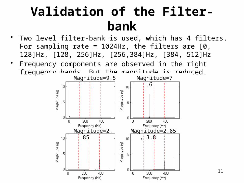
Validation of the Filter-bank• Two level filter-bank is used, which has 4 filters. For sampling rate = 1024Hz,

the filters are [0, 128]Hz, [128, 256]Hz, [256,384]Hz, [384, 512]Hz• Frequency components are observed in the right frequency bands. But the

magnitude is reduced.

11

Magnitude=9.5 Magnitude=7.6

Magnitude=2.85 Magnitude=2.85, 3.8

Spectral Kurtosis

12

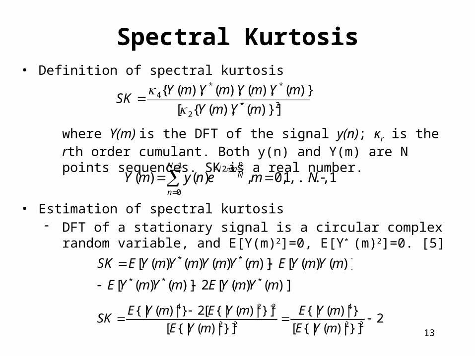
Spectral Kurtosis• Definition of spectral kurtosis

2*2

**4

)}](),({[

)}(),(),(),({

mYmY

mYmYmYmYSK

13

2}]|)({|[

}|)({|

}]|)({|[

}]|)({|[2}|)({|22

4

22

224

mYE

mYE

mYE

mYEmYESK

• Estimation of spectral kurtosis- DFT of a stationary signal is a circular complex random variable, and

E[Y(m)2]=0, E[Y* (m)2]=0. [5]

where Y(m) is the DFT of the signal y(n); κr is the rth order cumulant. Both y(n) and Y(m) are N points sequences. SK is a real number.

1,...,1,0,)()(1

0

2

NmenymY

N

n

N

nmi

)]()([2)]()([

)]()([)]()()()([***

**

mYmYEmYmYE

mYmYEmYmYmYmYESK

Result of SK• The SK have small value for white noise and high values for periodic signal.

- White noise, SK = -0.0406

- Pure periodic signal , SK = 510

14

Simulated Annealing

15

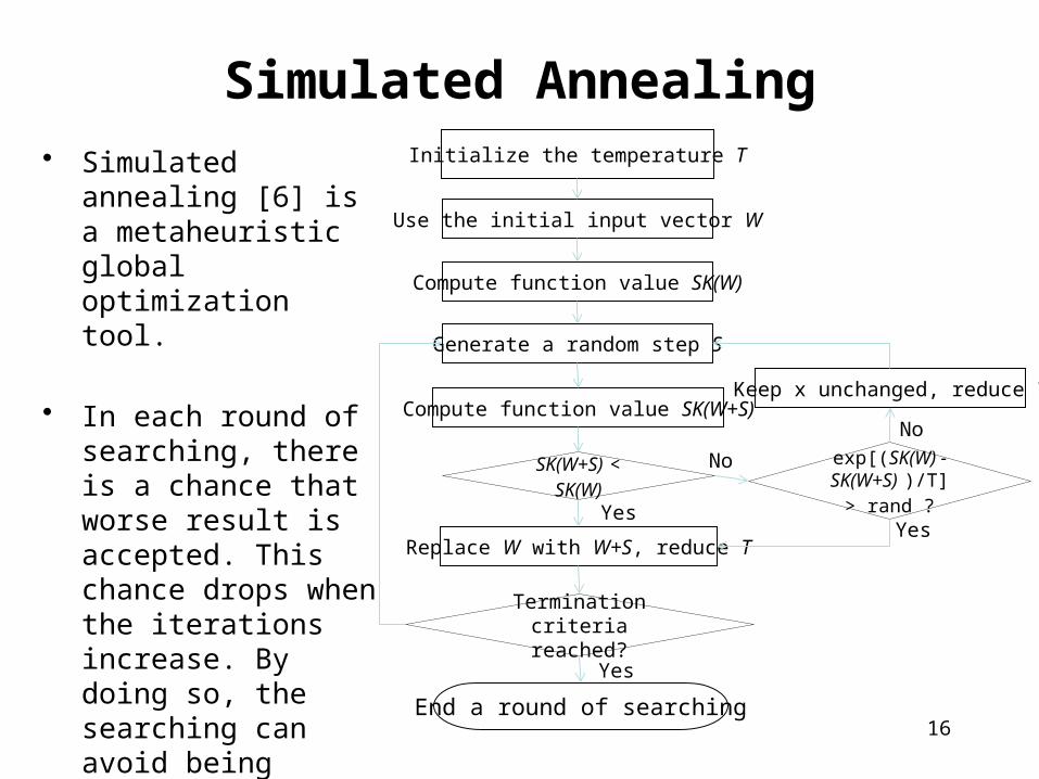
• Simulated annealing [6] is a metaheuristic global optimization tool.

• In each round of searching, there is a chance that worse result is accepted. This chance drops when the iterations increase. By doing so, the searching can avoid being trapped in a local extremum.

Initialize the temperature T

End a round of searching

Use the initial input vector W

Compute function value SK(W)

Generate a random step S

Compute function value SK(W+S)

SK(W+S) < SK(W)

exp[(SK(W) - SK(W+S) )/T] >

rand ?

Termination criteria reached?

Replace W with W+S, reduce T

Keep x unchanged, reduce T

Yes

No

Yes

Yes

No

Simulated Annealing

16

Validation of SA: 1-D Function• One dimensional function optimization

- The function has a global minimum and many local minimums.- The function is used to check the fundamental of the algorithm.- The global minimum is y=-100 when x= π

17

2)()cos(100 xxy

-10 0 10 20

-100

0

100

200

x

y

Initialize the temperature T

End a round of searching

Use the initial input vector W

Compute function value SK(W)

Generate a random step S

Compute function value SK(W+S)

SK(W+S) < SK(W)

exp[(SK(W) - SK(W+S) )/T] >

rand ?

Termination criteria reached?

Replace W with W+S, reduce T

Keep x unchanged, reduce T

Yes

No

Yes

Yes

No

Setting of the SA

18

T = 1000

W: A random number in [-10,10]

S: A random number in [-10,10]

T = 0.99T

T = 0.99T

1,000 iterations

Validation of SA: Result

19

• Result- SA ends at 1,000 iterations. The optimum is found at 943th iteration.- The minimum found is -99.9996, - Optimum variable x= 3.1389

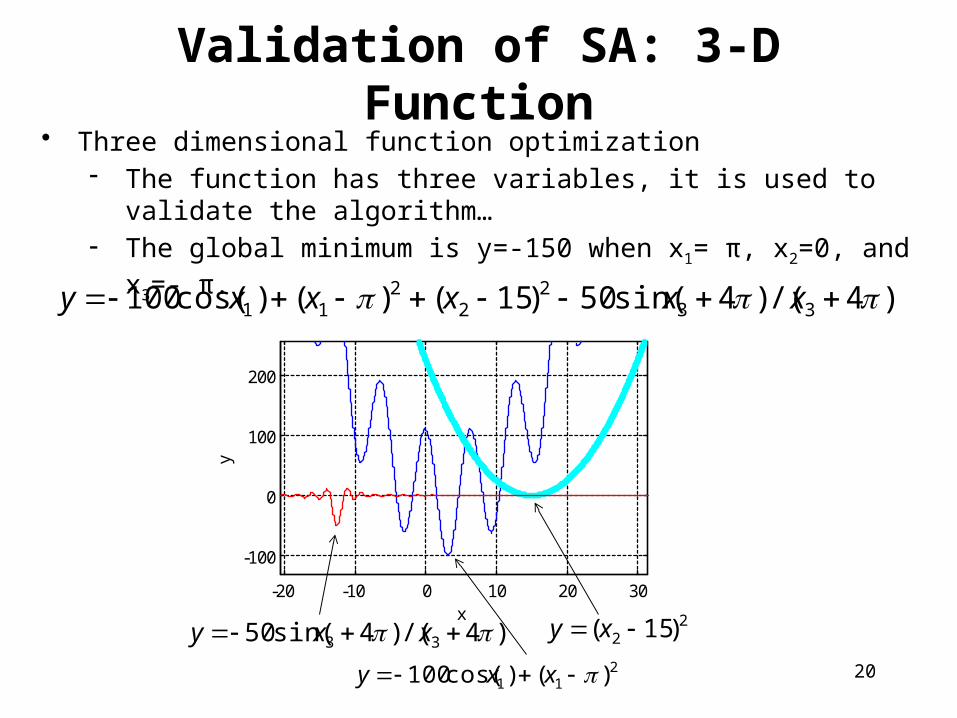
• Three dimensional function optimization- The function has three variables, it is used to validate the algorithm…- The global minimum is y=-150 when x1= π, x2=0, and x3=- π.

20

)4/()4sin(50)15()()cos(100 332

22

11 xxxxxy

-20 -10 0 10 20 30

-100

0

100

200

x

y

211 )()cos(100 xxy

22 )15( xy)4/()4sin(50 33 xxy

Validation of SA: 3-D Function

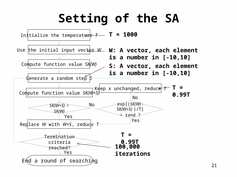
Initialize the temperature T

End a round of searching

Use the initial input vector W

Compute function value SK(W)

Generate a random step S

Compute function value SK(W+S)

SK(W+S) < SK(W)

exp[(SK(W) - SK(W+S) )/T] >

rand ?

Termination criteria reached?

Replace W with W+S, reduce T

Keep x unchanged, reduce T

Yes

No

Yes

Yes

No

Setting of the SA

21

T = 1000

W: A vector, each element is a number in [-10,10]

S: A vector, each element is a number in [-10,10]

T = 0.99T

T = 0.99T

100,000 iterations

22

Validation of SA: Setting and Result• Result

- SA ends at 100,000 iterations. The optimum is found at 76,455th iteration.- The minimum found is -149.5179- Optimum variable x= [3.1437 15.6941 -12.5659]

Envelope Analysis

23

• The enveloped signal is obtained from the magnitude of the analytic signal.• The analytic signal is constructed via Hilbert transform.

• Hilbert transform shifts the signal by π/2 via the following formula

• The analytic signal is constructed

• Magnitude of the analytic signal forms the enveloped signal.

dthyty oo )()()(ˆ

0.032 0.033 0.034 0.035 0.036 0.037 0.038-0.5

0

0.5

Time(s)

Am

plit

ude

tth

1

)(

Original signal

)(ˆ)()( tyjtyty ooa

|)(|)( tyta a

Hilbert transform of the original signal

Enveloped signal

Envelope Analysis

24

• A modulated signal y is used to validate the algorithm.

Validation of Envelope Analysis: Test Signal

25

200Hz

190Hz 210Hz

21 )1( xxy )102cos(1 tx

)4/2002cos(1002 tx

• After envelope analysis, modulating signal is obtained with a different magnitude.

• After FFT, the modulating frequency component is obtained.

Validation of Envelope Analysis

26

10Hz

Progress• October

- Literature review; exact validation methods; code writing• November

- Middle: code writing- End: Validation for envelope analysis and spectral kurtosis

• December- Semester project report and presentation

• February- Complete validation

• March- Adapt the code for parallel computing

• April- Validate the parallel version

• May- Final report and presentation

27

Remaining Work at this Stage

• Complete the validation of spectral kurtosis.• Put the sub-programs together to a single program.• Validate the whole program.

28

References

[1] Wind Stats Newsletter, 2003–2009, vol. 16, no. 1 to vol. 22, no. 4, Haymarket Business Media, London, UK [2] H. Link; W. LaCava, J. van Dam, B. McNiff, S. Sheng, R. Wallen, M. McDade, S. Lambert, S. Butterfield, and F. Oyague,“Gearbox Reliability Collaborative Project Report: Findings from Phase 1 and Phase 2 Testing", NREL Report No. TP-5000-51885, 2011

[3] Plane crash information

http://www.planecrashinfo.com/1987/1987-26.htm

[4] J. Antoni, “The spectral kurtosis: a useful tool for characterising non-stationary signals”, Mechanical Systems and Signal Processing, 20, pp.282-307, 2006

[5] P. O. Amblard, M. Gaeta, J. L. Lacoume, “Statistics for complex variables and signals - Part I: Variables”, Signal Processing 53, pp. 1-13, 1996

[6] S. Kirkpatrick, C. D. Gelatt, and M. P. Vecchi, "Optimization by Simulated Annealing". Science 220 (4598), pp. 671–680, 1983

29