locally orderless tracking - tau

Int J Comput VisDOI 10.1007/s11263-014-0740-6

Locally Orderless Tracking

Shaul Oron · Aharon Bar-Hillel · Dan Levi ·Shai Avidan

Received: 30 April 2012 / Accepted: 13 June 2014

Abstract Locally Orderless Tracking (LOT) is a visual tracking algorithm that automati-cally estimates the amount of local (dis)order in the target. This lets the tracker specializein both rigid and deformable objects on-line and with no prior assumptions. We providea probabilistic model of the target variations over time. We then rigorously show that thismodel is a special case of the Earth Mover’s Distance (EMD) optimization problem wherethe ground distance is governed by some underlying noise model. This noise model has sev-eral parameters that control the cost of moving pixels and changing their color. We developtwo such noise models and demonstrate how their parameters can be estimated on-line dur-ing tracking to account for the amount of local (dis)order in the target. We also discuss thesignificance of this on-line parameter update and demonstrate its contribution to the perfor-mance. Finally we show LOT’s tracking capabilities on challenging video sequences, bothcommonly used and new, displaying performance comparable to state-of-the-art methods.

Keywords Tracking · EMD

S.OronTel Aviv UniversityTel Aviv 69978, IsraelE-mail: [email protected]

A.Bar-HillelMicrosoft Research, Advanced Technology Labs Israel MicrosoftHaifa RD Center, Building No. 23, Matam, Haifa 31905, IsraelE-mail: [email protected]

D.LeviGeneral Motors Advanced Technical CenterHamada 7, Herzliya, IsraelE-mail: [email protected]

S.AvidanTel Aviv UniversityTel Aviv 69978, IsraelE-mail: [email protected]

2

1 Introduction

When addressing the visual tracking problem one often makes an explicit or implicit as-sumption about the type of target being tracked, treating it as either a rigid object or adeformable one. For example, when tracking a rigid object, where the only change in ap-pearance is due to rigid geometric transformations, it is reasonable to use a method such astemplate matching where the location of pixels is fixed and governed by a geometric trans-formation and similarity is reduced to per-pixel intensity difference. If, on the other hand,the object is extremely deformable, then tracking based on color histogram matching mightbe more suitable reducing the similarity between target and candidate to similarity betweentheir color distributions.

In this work we present a novel visual tracking algorithm we call Locally OrderlessTracking (LOT). This algorithm uses a joint spatial-appearance space representation andis able to estimate, on-line, the amount of local (dis)order in the target. Thus if the targetis rigid and there is little or no local disorder then LOT preserves spatial information liketemplate matching. However, if the target is nonrigid, LOT disregards spatial information asin histogram matching.

The first contribution of our work is a new probabilistic interpretation of the EarthMover’s Distance (EMD) that we name Locally Orderless Matching (LOM). Using thisinterpretation one can calculate the likelihood of patch P being a noisy replica of patch Qwhere noise can be introduced by change in the spatial order of pixels in the patch, changein their appearance, or both. In other words, LOM infers the probability Pr(P |Q,Θ) whereΘ are noise model parameters, some of which control the cost of moving pixels spatiallywhile others control the cost of changing a pixels appearance, for example due to illumi-nation variation. Since our derivation is general one can plug in any noise model into thisframework and we demonstrate the use of two such noise models.

The second contribution of our work is introducing Locally Orderless Tracking whichapplies Locally Orderless Matching to visual tracking. Locally Orderless Tracking is a par-ticle filter based tracker that uses Locally Orderless Matching to infer the likelihood of eachobserved particle being a noisy replica of the target. Particles are represented as signaturesin a joint spatial-appearance space, using superpixels for better efficiency. Key to our ap-proach is the ability to adapt to both rigid and deformable targets. This ability is obtainedby an on-line noise model parameter estimation scheme driven by the LOM solution. Thisadaptation is a fully automated process that requires no user intervention.

This work is an extension of Oron et al. (2012), providing additional experiments andmore discussions.

The rest of this paper is organized as follows. Section 2 covers related work. Section 3presents Locally Orderless Matching. Section 4 discusses noise models. Section 5 introducesLocally Orderless Tracking. Section 6 covers experiments and we conclude in section 7.

2 Related Work

We are inspired by the work of Koenderink and Van Doorn (1999) on the structure of lo-cally orderless images which proposes an image representation method where the amountof spatial order preserved globally and locally can be tuned using two parameters. This rep-resentation was shown by Ginneken and Haar Romeny (1999) to be useful for applicationssuch as adaptive histogram equalization, noise removal and segmentation. In our case, wewish to determine the optimal extent of local disorder of the data for the purpose of tracking.

3

In rigid object tracking one usually attempts to exploit spatial information in the objectby using template based methods. In some cases the template is used in a simple manner(Hager and Belhumeur (1998)) while others use multiple templates and sparse representa-tions (Ross et al. (2004, 2007); Mei et al. (2011); Kwon and Lee (2010)). These approachesoffer good stability and can handle occlusions and scale estimation but are less suitable forhandling non-rigid deformations and dynamics such as out-of-plane-rotations.

When tracking deformable objects one often uses histogram representations (Comaniciu(2002)) or discriminative methods that treat the problem as a pixel-wise binary classificationproblem (Godec et al. (2011); Avidan (2005); Grabner et al. (2006)). These approachesmostly disregard spatial order, and can therefore handle difficult non-rigid transformations.However they are more prone to drift and are often less stable especially at scale estimationor occlusion handling.

Some attempt to combine rigid and deformable object approaches. For example Wanget al. (2011) use mid level cues that capture spatial information to some extent while Santneret al. (2010) heuristically combine discriminative and generative components . However,unlike LOT, these methods do not measure nor adapt to local disorder in the data in anexplicit manner.

The work most related to ours is that of Elgammal et al. (2003), proposing a trackerthat uses a joint spatial-appearance space and can specialize to either histogram trackingor sum-of-square-difference (SSD) tracking by an off-line adjustment of parameters. Theproposed method is significantly different in several ways. First and foremost, due to theon-line parameter estimation which enables LOT to specialize in rigid template trackingor deformable object tracking on-line and secondly due to the use of Particle Filtering andEMD instead of the kernel based gradient decent approach of Elgammal et al.

The Earth Mover’s Distance (EMD) has a long history in computer vision. EMD wasfirst considered by Peleg et al. (1989) as an image similarity metric and popularized byRubner et al. (2000) (who coined the name) for content based image retrieval. A proba-bilistic analysis of EMD and its relation with the Mallows distance was proposed by Levinaand Bickel (2001) although that analysis differs from the proposed probabilistic frameworkwhich introduces a noise process that governs the ground distance in the EMD. Recently,Zhao et al. (2010) proposed a differential EMD approach that derives a gradient descentmethod to find the object location quickly using the EMD as a similarity measure. How-ever, the focus of that paper is on using EMD to handle illumination changes, the object isrepresented as a color signature and no consideration is given to pixels inner location in thetemplate.

Generative probabilistic Bayesian approaches also known as Particle Filters or Sequen-tial Monte Carlo (Doucet et al. (2001)) are widely used for visual tracking (Kwon and Lee(2010); Ross et al. (2007)). In our work we closely follow the Condensation algorithm pro-posed by Isard and Blake (1998) which suggest a Particle Filtering technique using factoredsampling.

Superpixels first proposed by Ren and Malik (2003) have been used in recent years formany computer vision applications such as segmentation and classification (Hoiem et al.(2005); He et al. (2006)) and tracking (Wang et al. (2011)). In our work, similar to Boltzet al. (2010), superpixels are used to reduce the computational cost of EMD.

We refer interested readers to a thorough survey of the vast work in visual tracking doneby Yilmaz et al. (2006).

4

3 Locally Orderless Matching

Locally Orderless Matching measures the similarity between two images or two imagepatches based on the EMD. Pixels are represented in a joint spatial-appearance domain.For appearance we use color values but other descriptors such as gradients or local texturecan also be used. For position pixel coordinates in a patch, normalized to the range [0, 1],are taken. A pixel is represented as pi = (pLi , p

Ai ) where pLi = (x, y) is the pixels location

and pAi ∈ RD its appearance.We want to probabilistically explain a candidate patch P as a noisy replica of the tem-

plate Q. We begin by looking at the pixel-wise inference problem, where patches P and Qare treated as sets of pixels, and show that in this case the problem is equivalent to a form ofEMD optimization problem. We then propose using signature representations for P and Qin which pixels are clustered together using superpixel segmentation and claim the problemcan now be formulated as the signature EMD problem (Rubner et al. (2000)). This is donein order to reduce the computational cost of EMD and we justify it by bounding the errorresulting from the related coarsening of the representation.

Let us consider patches P and Q as sets of pixels. We start with a probabilistic perspec-tive of EMD and wish to show that it measures the conditional probability of one set, giventhe other set and model parameters. Formally, denote the two sets by P = {pi}ni=1, Q =

{qi}ni=1, and assume that we have a probabilistic model stating the probability that a spe-cific element p ∈ P originated from a specific element q ∈ Q, Pr(p|q,Θ), with Θ the modelparameters. We want to extend it to the conditional probability between the sets Pr(P |Q,Θ).

The extension relies on a hidden 1:1 mapping between elements of P and Q. Denotesuch a mapping by h : {1, .., n} → {1, .., n} with h(i) = j meaning that element pi wasgenerated from element qj . We can get the probability of P being generated from Q bymarginalizing over the possible hidden assignments (dropping Θ from the notation as it iscurrently constant):

Pr(P |Q) =∑h

Pr(P |Q,h)Pr(h) (1)

Assuming a uniform prior over the h’s (no reason to assume anything else) we have:

Pr(P |Q) =1

n!

∑h

Pr(P |Q,h) (2)

Approximating the average using maximum a posteriori (MAP) estimation, i.e. assumingthe sum is dominated by the highest term (the best hidden map) we get:

Pr(P |Q) ∼ c ·maxhPr(P |Q,h) (3)

Dropping the constant c, assuming independence between the set elements and taking thelogarithm we get:

logPr(P |Q) ∼ maxhlogPr(P |Q,h)

= maxh

∑ni=1 logPr(pi|qh(i), Θ)

(4)

5

Proposition 1 Optimization problem (4) is the signature EMD problem EMD(P,Q,d) for thefollowing signatures and ground distance:

P = {(p1, 1), (p2, 1), . . . , (pn, 1)}Q = {(q1, 1), (q2, 1), . . . , (qn, 1)}d(p, q) = −logPr(p|q,Θ)

(5)

Where the signatures are comprised of objects, e.g. (pi, wi), each having a description piand weight wi. In our case the signatures are simply collections of all the pixels in patchesP and Q equally weighted.

Proof Starting with Equation (4) we have:

maxh

∑ni=1 logPr(pi|qh(i), Θ) =

minh

∑ni=1−logPr(pi|qh(i), Θ) =

minh

∑ni=1 d(pi, qh(i))

(6)

where the mapping h can be expressed as a permutation matrix F in which fij = 1 iff h(i) =j. Denoting dij = d(pi, qj) the problem statement becomes:

min∑i,j fijdij

such that ∑i fij = 1,

∑j fij = 1, fij ∈ {0, 1}

(7)

If we put this integer linear programming problem in the canonical form {min c · x|Ax =

b, x ≥ 0} we find that the matrix A is totally unimodular (Heller and Tompkins (1956)).This implies the linear programming problem in which we relax the constraint fij ∈ {0, 1}to fij ≥ 0 has an integral optimum, meaning the constraint can be relaxed without changingthe result.

The linear programming problem obtained by this relaxation is identical to the one ob-tained for signature EMD with identical mass as presented by Rubner et al. (2000).

min∑i,jfijdij

such thatfij ≥ 0,

∑i fij ≤ wqj ,

∑j fij ≤ wpi∑

i,jfij = min(

∑i wpi ,

∑j wqj )

(8)

Where in our case all wpi and wqj are equal to 1. In which case the inequalities∑i fij ≤

wqj ,∑j fij ≤ wpi can be replaced by equalities and then the last constraint can be dropped.

ut

In other words, conditional set probability, under 1:1 mapping and element indepen-dence assumptions, is equivalent to signature EMD with singleton bins. However, the equiv-alence naturally extends to conditional probabilities with P and Q containing repeating ele-ments and signature EMD with general integer bin quantities.

Proposition 2 Let

P = {(p1, wp1), (p2, wp2), . . . , (pn1 , w

pn1)}

Q = {(q1, wq1), (q2, wq2), . . . , (qn2 , w

qn2)}

(9)

6

be signatures for which we cluster repeating elements into single objects increasing theirweights accordingly (i.e. p1 appears wp1 ∈ N times in P , etc.). Solving the pixel matchingproblem for P and Q as formulated in optimization problem (7) (which has m2 variableswhere m =

∑ni=1 w

pi ) is equivalent to solving the EMD problem (8) for P and Q (which

has n1 · n2 variables) i.e. both problems have the same minima.

The proof of proposition 2 is given in the appendix. We see that when sets P and Q containidentical items it lowers the computational cost of the matching using EMD formulation.Hence clustering similar items and replacing them with a single object is an attractive ap-proximation to the likelihood. However this approximation degrades as the clustering be-comes coarser. We can bound this error in likelihood estimation as follows:

Proposition 3 Assuming that the ground distance d(p, q) is a metric.Let P = {(p1, wp1), . . . , (pn1 , w

pn1)} , Q = {(q1, wq1), . . . , (qn2 , w

qn2)} be two signatures

and let P , Q be crude versions of P,Q such that any object in P is created by unitingobjects in P and the same holds for Q,Q. Denote by hp, hq the functions mapping eachobject P,Q to its containing object in P , Q. Then:

|EMD(P,Q, d)− EMD(P , Q, d)| ≤∑n1

i=1 wpi d(pi, php(i)) +

∑n2

i=1 wqi d(qi, qhq(i))

(10)

In other words, the EMD approximation gap is bounded by the sum of distances betweenthe original cluster centers and their cruder counterparts in the crude signatures. The proofis given in the appendix.

4 Noise Model

We have shown that Locally Orderless Matching attempts to explain a set P as a noisyreplica of set Q, under some pixel-pair noise model with parameters Θ. We now present anddiscuss the Gaussian noise model for pixel-pairs. We give special attention to the parameterestimation scheme, demonstrating how these noise model parameters and their estimationallow our algorithm to adapt, on-line, to both rigid and deformable objects.

We note that since the derivation presented in section 3 is general with respect to thenoise model, any distribution can be used as a noise model. One can use prior knowledge,theoretical or empirical, about the noise to make an educated choice. Furthermore, since ourproblem is cast in term of probabilistic inference the noise model parameters can be inferredusing maximum-likelihood (ML) estimation based on the EMD solution, as we demonstratefor the models we present here.

We focus on the Gaussian noise model as it is simple and intuitive and also as it wasfound to be empirically superior to a second noise model we tested, as presented in section6.5. Information on additional noise models is provided in appendix A.

4.1 Gaussian Noise

A Gaussian distribution with zero mean and scalar covariance is considered for both lo-cation and appearance, assuming independence between the two, i.e. Pr(p|q,ΘL, ΘA) =

Pr(pL|qL, ΘL) · Pr(pA|qA, ΘA), in which case we have:

Pr(pL|qL) ∼ N(0, ΣL = σL · I)Pr(pA|qA) ∼ N(0, ΣA = σA · I)

(11)

7

Denoting Θ = (σL, σA). The conditional probability is:

Pr(p|q,Θ) =1

2πσ2Le− ||p

L−qL||222σ2L · 1

(2π)D/2σDAe− ||p

A−qA||222σ2A (12)

Ground distance in this case is:

d(p, q) =1

2σ2L||pL − qL||22 +

1

2σ2A||pA − qA||22 + C (13)

WhereC = D+22 log(2π)+2log(σL)+Dlog(σA). This model is simple and intuitive, closely

related to Koenderink and Van Doorn (1999) locally orderless image representation.Observing equation (13) it is easy to see that if σA >> σL the ground distance is

dominated by the first term, i.e. the cost of moving a pixels spatially is much higher than thecost of appearance errors. In this case the optimal EMD solution would leave all the pixelsin place, reducing to a sum-of-square-difference, as in rigid template matching. If howeverσL >> σA then the ground distance is dominated by the second term, making it very costlyto change pixels appearance compared with moving them spatially. In this case all spatialinformation is lost and the EMD is reduced to histogram matching (in the EMD sense).

This property is key to LOT’s ability to adapt to both rigid and deformable targets. More-over, since the noise model parameter update is done on-line, based on the EMD solutionobtained at each frame, the “rigidity” adaptation is also done on-line in a fully automaticmanner requiring no user intervention and very little parameter tuning.

4.1.1 Gaussian Noise Parameter Estimation

Locally Orderless Matching with a Gaussian noise model of the form discussed above hastwo parameters σA and σL. Due to the independence assumed between appearance and lo-cation each parameter can be estimated separately using the same Maximum Likelihood(ML) estimator. Therefore, p, q, σ,D will be used without the superscripts A,L. Recallfrom propositions 1,2 that logPr(P |Q,Θ) ∼

∑i,jdijfij , where the fij providing the map-

ping, are obtained from the EMD solution. Maximum likelihood can hence be obtained bydifferentiating

∑i,jdijfij with respect to σ and comparing to zero. For dij = d(pi, qj) =

12σ2 ||pi − qj ||22 + D

2 log(2π) +Dlog(σ) we get:

σ2 =1

D

∑i,jfij ||pi − qj ||22∑

i,jfij

. (14)

5 Locally Orderless Tracking

Locally Orderless Tracking applies Locally Orderless Matching to tracking. This is done ina Baysian approach using Particle-Filtering (PF) where the likelihood that a certain particlehas originated from the tracked object is inferred using Locally Orderless Matching. Theoverall algorithm is given in Algorithm 1. Specific details are provided below.

8

Algorithm 1 Locally Orderless Tracking

Input: Frame I(n), target signature Q0 = {qi, wqi }MQ0i=1 , noise parameters Θ(n−1), particle states

{X(n)k }

Nk=1

Output: New target state X(n)Target, updated parameters Θ(n), new particle states {X(n+1)

k }Nk=1

1. Partition ROI in I(n) into superpixels ISP2. For each particle X(n)

k do:

(a) Build signature P (n)k = {pki , w

pk

i }MPki=1 using ISP

(b) Compute ground distances:{dk}ij = d(pki , qj) = −log(pki |qj , Θ(n−1))

(c) Compute EMDk ← EMD(P(n)k , Q0, dk)

(d) Compute particle weight according to (17)3. Find new target state X(n)

Target according to (18)

4. Build target signature P (n)Target and ground distance dTarget

5. Compute EMD flow fi,j ← EMD(P(n)Target, Q0, dTarget)

6. Update parameters Θ(n) according to (19).7. Create new particle set {X(n+1)

k }Nk=1 using the Condensation algorithm Isard and Blake (1998).

We use a Bayesian tracking formulation where the goal is to find the most probable stateat frame n denoted X(n)

Target. This state in our case is a rectangle defined by (x, y, w, h).

Given some particle state at frame n, X(n)k and the observations up to frame n , Z(1:n)

k ,which are the signatures associated with that state. We assume that target dynamics forma temporal Markov chain so that Pr(X(n)

k |X(n−1)k , . . . , X

(1)k ) = Pr(X

(n)k |X

(n−1)k ). We

would like to estimate the posteriori probability Pr(X(n)k |Z

(1:n)k ). Using Bayesian formu-

lation we have:

Pr(X(n)k |Z

(1:n)k ) = c

(n)k · Pr(Z(n)

k |X(n)k )Pr(X

(n)k |Z

(1:n−1)k ) (15)

where

Pr(X(n)k |Z

(1:n−1)k ) =

∫Pr(X

(n)k |X

(n−1)k )Pr(X

(n−1)k |Z(1:n−1)

k )dX(n−1)k (16)

and c(n)k is a normalization constant that does not depend on X(n)k . Computing equation

(15) requires multiplying the observation density Pr(Z(n)k |X

(n)k ) by the effective prior

Pr(X(n)k |Z

(1:n−1)k ). This effective prior term is generated based on the process dynam-

ics which determine Pr(X(n)k |X

(n−1)k ) and using the posterior from the previous time step

Pr(X(n−1)k |Z(1:n−1)

k ) which will be discussed later. The observation density in (15) is in

fact the probability Pr(P (n)k |Q0, Θ) inferred using LOM, where P (n)

k is the correspondingpatch representation for the k’th particle in the n’th frame and Q0 is our target patch rep-resentation. To define this conditional probability between patches we only have to definethe probabilistic noise model for single pixels Pr(p|q,Θ). Then the ground distance for theEMD is defined as d(p, q) = −log(p|q,Θ) and Pr(P (n)

k |Q0, Θ) is obtained by solving theEMD problem.

Since solving an EMD problem can be a computationally challenging task, instead of us-ing raw pixel values we work with superpixels. Specifically, we use Levinshtein et al. (2009)

9

TurboPixels clustering algorithm to produce over segmentation in a region-of-intrest (ROI)which supports all the particle related patches. Candidate patches are then represented bysignatures which are generated from this superpixel image. A signature consists of M clus-ters that reside in the signature support, i.e. a rectangle. Each cluster is represented by itslocation , i.e. geometric center of mass (in patch canonical coordinates ranging [0, 1]), andaverage appearance (e.g. average HSV values). We note that each signature is normalizedto have unit weight. In this setup running LOM maps all the weight of the target patch tothe candidate patch. This does not result in a 1:1 mapping of superpixles nor pixels, sincetarget superpixels can be split into several candidate superpixels, also each patch might becomprised of a different number of pixels. This however does not pose a theoretical problem(see proposition 2) nor a practical one since solving the EMD optimization problem is stillfeasible and the flow obtained can still be used for parameter estimation.

The full Particle Filtering scheme we use follows closely the Condensation algorithmof Isard and Blake (1998). For each new frame that comes in we do the following: Builda signature for each of the N particles according to their state i.e. each particle representsa rectangular image patch. Then calculate the EMD between each of these candidate sig-natures {P (n)

k }Nk=1 and the target signature Q0 with ground distances as explained above

(calculated using the noise model parameters Θ). The EMD scores {EMD(n)k }

Nk=1 are then

used to set particle weights according to:

π(n)k =

e−β·EMD(n)k∑N

k=1 e−β·EMD

(n)k

(17)

We now have a set of weighted particle states {X(n)k , π

(n)k }

Nk=1 with which we do two things.

The first is compute the final state X(n)Target according to:

X(n)Target = E[X(n)] =

N∑k=1

X(n)k · π(n)k (18)

The second thing we do with this weighted particle set is create a new particle set for thenext frame that comes in. This is done as described in Isard and Blake (1998) by samplingparticles from the current weighted set (with probability proportional to their weight) thensubjecting them to a prediction phase according to the process dynamics which also includesome random noise process. This factored sampling process uses Pr(X(n−1)

k |Z(1:n−1)k ) in

order to produce a particle set approximating the required Pr(X(n)k |Z

(1:n−1)k ).

Finally the last step of each iteration is noise model parameter update based on thenew target state found. This stage is carried out as follows. We begin by building P (n)

Target

the signature for our new target state X(n)Target. Then we compute the EMD flow between

this signature and the target signature Q0 providing the most probable mapping betweensource and target signatures. Using this flow we estimate the noise distribution parametersΘ

(n)ML according to what is described in section 4. These estimated parameters are then

regulated using a prior ΘPrior and a moving average (MA) process before producing thefinal parameters Θ(n):

Θ(n)MAP =

Θ(n)ML+ΘPrior·wPrior

1+wPrior

Θ(n) = (1− αMA) ·Θ(n−1) + αMA ·Θ(n)MAP

(19)

10

We emphasize that noise model parameters reflect the degree of rigidity in the target,thus on-line noise model parameter update enables LOT to adapt to different types of targets.

Although we do not update the target template explicitly, noise parameter update can beviewed as a limited form of template update. This is because setting noise model parametersdirectly affects the EMD solutions space thus effectively changing the space of possiblematches.

We note that currently our algorithm does not handle occlusions explicitly, however par-tial occlusions are handled quite well due to two mechanisms: one is the use of particlefiltering which allows locking back to a target after it was lost due to an occlusion. Addi-tionally since in many cases the visible part of an occluded target shares its color statisticswith the entire target, LOT can reduce to tracking only the visible part of the target, allowingit to overcome partial occlusions.

6 Experiments

This section presents experimental results. We begin with a synthetic experiment demon-strating noise parameter estimation in a simplified scenario. Then we present the experi-mental setup, parameter configurations, data-sets and performance evaluation method thatwill be used throughout the rest of the experimental section. We present the on-line param-eter estimation of LOT on both a toy-example and real data, followed by an experimentillustrating the significance of updating the noise parameters on-line using benchmark se-quences. We then consider two noise models and compare their performance after which wepresent quantitative results comparing LOT with 6 state-of-the-art tracking algorithms.

6.1 Synthetic Noise Model Parameter Estimation Experiment

The following synthetic experiment demonstrates parameter estimation for the Gaussiannoise model in a simplified scheme. We estimate the noise in location σL and the noisein appearance σA. This estimation is done in a Maximization-Maximization (MM) schemewhere we solve the EMD then estimate the noise model parameter using an ML estimator,we then use these parameters to solve the EMD again and so on until both EMD and param-eters converge. We note that convergence to a local maxima is guaranteed as both MM steps(i.e. EMD and ML) increase the likelihood.

Figure 1 shows the result of two such experiments. We started with an image over-segmented into super-pixels and coarsened it appropriately. This coarsened image was con-taminated by two types of noise. In the first case additive-white-Gaussian-noise (AWGN),σA = 0.4, was added to the cluster appearances. σA was also empirically calculated from theknown cluster correspondence (σEmpiricA = 0.417). We performed parameter estimation us-ing our MM scheme allowing both σL and σA to vary (starting from σL = 0.05, σA = 0.05)and found that σA converged to 0.396 . For better visualization of the results we coloredeach cluster of the noisy image according to the coarsened image cluster which contributedthe maximal amount of weight to it based on the EMD flow. For comparison, we repeatedthe experiment with randomly chosen parameter values σL = 0.35, σA = 0.11 (drawn uni-formly from the interval [0, 0.5]), and found that using the estimated parameters producesbetter visual results.

In the second case cluster appearances were locally permutated (i.e. cluster colors wereswapped) to produce localization noise. This time σL was empirically calculated using

11

(a) Input (b) Noisy versions (c) Correct matches (d) Wrong matches

Fig. 1 Synthetic Experiment : (a) Original image with super-pixel boundaries (top) and image coarsenedinto super pixels (bottom) (b) Coarsened image with additive-white-Gaussian-noise added to the color of thesuper pixels (top) and super-pixel appearance permutation (bottom). (c) Matching found of images in (b) tocoarsened image using estimated σA, σL (top/bottom accordingly). Colors projected from coarsened image.(d) Matching found of images in (b) to coarsened image using random σA, σL (top/bottom accordingly).Colors projected from coarsened image.

Fig. 2 In blue: Values of σA estimated using Maximization-Maximization (MM) vs. empirical values calcu-lated based on known noise values. Contaminating noise was additive-white-Gaussian-noise (AWGN), withdifferent variance values, added to cluster appearance. In red: σL values estimated using MM vs. empiri-cal values calculated based on known noise (permutation). Localization noise was modeled as local clusterappearance permutation i.e. swapping cluster colors in different neighborhood sizes.

the known correspondence (σEmpiricL = 0.497) and compared to our estimated parame-ters (same initialization) calculated without knowing the permutation. Again, our estima-tions converged correctly to the value σL = 0.492, taking σA → 0 . Colors were pro-jected as explained before to demonstrate the advantage over using random parameter values(σL = 0.28, σA = 0.32).

12

This experiment was repeated for 2 additional σA and σL values. Figure 2 presents thevalues of σA, σL found using our MM estimation versus empirical values measured fromthe actual noises. The graphs show we can consistently estimate the parameters correctly fora wide range of noises.

We conclude that parameter estimation based on the EMD solution can produce resultshighly correlated with the contaminating noises at least in the case of the Gaussian noisemodel.

6.2 Experimental Setup

In the experiments reported here HSV color space is used for appearance description. Bothappearance and location spaces are used in a canonical form, i.e. normalized to the range[0, 1]. Cluster weights are determined according to the fraction of pixels associated withthem in the signature (thus ensuring a total signature weight of 1). The state vector includesposition and scale, i.e. Xi = (xi, yi, wi, hi), and a zero-order motion model is assumedthus the process model for the Condensation algorithm includes only effects of noise. For xand y the process noise is additive-white-Gaussian-noise (AWGN) with σxy = 7. For scaleparameters w and h we use multiplicative-Gaussian-noise with mean 1 and σwh = 0.07

(i.e. STD reflecting 7% scale change). The noise is added to each of the state variablesindependently. We use N = 250 particles with particle weighing parameter β set to 10 inorder to better differentiate between particle scores.

Superpixels are built in a ROI that supports all the particles. The desired number of su-perpixels (a parameter of the Turbopixel algorithm) is set in the range 300− 1000 where theactual value is determined such that the target region would consist of roughly 20 superpix-els. All the parameters are kept fixed for all experiments.

Using a standard PC equipped with an Intel Core i7 processor our Matlab-Mex imple-mentation runs at ∼ 1 frame per second for a target window size of ∼ 50 × 50 pixels. Therun time is divided almost equally between two major time consuming operations which arethe superpixel clustering and the EMD calculation for all the particles.

Our evaluation dataset is comprised of two subsets. The first includes 9 commonly usedsequences (5 color and 4 grayscale) appearing in recent related publications (Ross et al.(2004, 2007); Babenko et al. (2009); Mei et al. (2011); Kwon and Lee (2010); Wang et al.(2011); Santner et al. (2010)). The second subset presents 6 challenging new sequences in-cluding gray-scale and color examples with both static and moving cameras. The targetsin these sequences are subject to many appearance changes due to different types of de-formations, pose changes, out-of-plane-rotations, massive scale changes, motion blur andillumination changes.

We adopt the widely used PASCAL VOC (Everingham et al. (2010)) criterion whichquantifies both the centering accuracy as well as the scale accuracy. The criterion is a0 =area(Bp∩Bgt)area(Bp∪Bgt) where Bp and Bgt denotes the predicted and ground truth bounding boxesaccordingly. Successful tracking is considered as a0 > 0.5 (50%). We note that some ofthe sequences were re-annotated in order to provide ground truth for each frame that alsoaccounts for scale changes disregarded in some of the original annotations.

13

6.3 On-line Parameter Update

Before we start the performance evaluation on the main dataset we would like to firstdemonstrate the on-line noise parameter update capabilities of LOT. We begin with a 500

frame toy-example of a LEGO target subject to both appearance and localization noises.We use the Gaussian noise model which means Gaussian noise for both appearance andlocalization (as presented in section 4.1). This Gaussian model has two parameters i.e.Θ = {σA, σL} which are updated according to (19). Parameters are initialized accordingto σAprior = 0.05, σLprior = 0.1, with prior weights set to w

σpriorA= w

σpriorL= 0.25. The

ML estimators are calculated according to equation (14) and the MA parameter is fixed toαMA = 0.3. Figure 3 presents the behavior of the noise parameters σL and σA and sample

50 100 150 200 250 300 350 400 450 5000

0.05

0.1

0.15

0.2

0.25

0.3

Frame

σ

135

290

420

σA

σL

Frame 1 Frame 135 Frame 290 Frame 420

Fig. 3 Parameter estimation for the LEGO sequence: (Top) Noise parameter values, σL (Dashed-Red) andσA (Solid-Blue) per frame showing their on-line update.(Bottom) Four sample frames. First the target isilluminated with a strong light causing an appearance change handled by increasing σA. Next the targetis rotated and since we only model 2D translation (w/o rotation) this creates localization noise which ishandled by a large σL variation. Finally the target moves away from the camera causing a scale changewhich is correctly tracked without significant noise parameter changes.

frames for the LEGO sequence. The target is first subject to an illumination change. LOTdetects the appearance change and increases the appearance noise parameter σA while main-taining perfect tracking. As the illumination returns to normal the value of σA decreases.Next the target is rotated about its origin. The tracker state space does not include rotationtherefore this rotation is effectively localization noise. As before the target is tracked per-fectly while LOT estimates and adapts the value of σL on-line, increasing σL as the rotationangle increases and then decreasing σL as the target is rotated back. Towards the end ofthe sequence the algorithm correctly tracks target scale changes without altering the noiseparameters which is a desired behavior.

We proceed to demonstrate the on-line parameter update using two sequences from ourdataset. Figure 4 presents the noise parameter values as well as sample frames for the Dogand Shirt sequences. For the Dog sequence (Top) we observe that as there are no illuminationor other appearance changes the value of σA remains low and almost constant throughoutthe entire sequence. The value of σL on the other hand is updated due to localization noise

14

200 400 600 800 1000 12000

0.05

0.1

0.15

0.2

0.25

Frame

σ

280

1048

1200

σA

σL


100 200 300 400 500 600 700 800 900

0.08

0.09

0.1

0.11

0.12

0.13

0.14

0.15

Frame

σ

517

601

850

σA

σL


Fig. 4 Parameter estimation for the Dog (upper half) and Shirt (bottom half) sequences demonstrating on-line noise parameter update. For each sequence, on top is Noise parameter values, σL (Dashed-Red) andσA (Solid-Blue) per frame showing their on-line update. On the bottom four sample frames. For the Dogsequence there are no appearance changes and mainly out-of-plane rotations which cause localization noiseaffecting only σL. For the Shirt we observe appearance noise dominates over localization noise explainingmotion blur and local self occlusions.

in the form of target out-of-plane rotations and scale changes that push part of the target outof the frame support.

For the Shirt sequence (bottom part of figure 4) we notice that both noise model pa-rameters are actively updated although σA dominates over σL. The main reasons for thisbehavior are: 1) the rapid movement of the shirt creates motion blur mixing the differentcolors creating appearance changes. 2) The waving of the bottom part of the shirt cause lo-cal deformations and self occlusions that most of the time do not affect the top-left part ofthe target (which does not suffer localization changes). Due to these reasons LOM tends toassociate matching errors with appearance changes rather than localization noise.

6.4 Significance of On-line Parameter Update

In order to point out the importance and significance of on-line parameter estimation wecompare the performance of LOT with and without on-line parameter update. To do so we

15

use the Gaussian noise model considering two fixed parameter configurations. In the firstconfiguration we fix σA = 0.05, σL = 0.2 making the cost of changing cluster appearancesmore expensive then the cost of changing a clusters locations. In the second configurationwe fix σA = 0.2, σL = 0.05 making appearance changes less costly compared with locationchanges. We evaluate the tracking performance as explained above using our full dataset (15sequences).

Table 1 Comparison of tracking performance with fixed noise parameters vs. on-line updating parameters.Table entries are the percent of frames for which the PASCAL criterion was a0 > 0.5. Best result are inbold preface. As can be seen on-line parameter estimation improves tracking performance in 12 out of 15sequences.

Sequence Dataset σA = 0.05, σL = 0.2 σA = 0.2, σL = 0.05 On-lineShop Common 33.6 33.6 34.6Girl Common 32.3 49.1 67.6Human Common 94.2 7.3 97.6Skating Common 13.4 15.6 29.4Lemming Common 67.4 56.4 73.8Dog Common 91.3 51.4 97.4David Common 8 3.5 10Sylv Common 48.7 2.6 46Face Common 42.5 21.7 44.4DH New 33.9 16.8 92.3Shirt New 75 60.9 88.1Train New 53.2 82 69.6UCSDPeds New 6.5 1.5 73.9Boxing New 72.8 55.7 70.1Towel New 97.3 93 99.7

Results presented in Table 1 demonstrate the significance of on-line parameter update.When using on-line update the algorithm outperforms the fixed parameter configuration in12 out of 15 cases. For some of these sequences performance with on-line update is closeto the best results produced by fixed parameters (e.g. Human and Face) while for othersequences on-line update allows better performance relative to both fixed parameter con-figuration (e.g DH, Skating and Girl) demonstrating the advantage of the on-line parame-ter updating scheme. Closely examining the remaining 3 examples where fixed parametersdo better (Sylv,Train,Boxing), we can see that for Sylv and Boxing fixed parameters, withσA = 0.05 and σL = 0.2, only give a marginal absolute improvement of less than 3%. Thusonly in one case (Train) fixed parameters, with σA = 0.2 and σL = 0.05, are able to producesubstantially better results than on-line updating parameters (82% vs. 69.6%). In this specificcase the performance gain is due to better behavior under several partial occlutions allowingthe fixed parameters to retain large overlap while the updating parameters cause the targetto shrink only to the visible part of the target. Overall, although on occasion fixed parameterconfigurations can lead to better performance, in general, fixed parameters lack the muchneeded flexibility to cope and explain different object types and different levels of targetrigidity. On-line parameter update grants us this adaptation flexibility which leads to bettertracking performance in most cases, many times exceeding what a single fixed parameterconfiguration can achieve.

16

6.5 Noise models

LOM derivation is general in the sense that any noise model can be plugged into this frame-work. The noise model controls the ground distance in the EMD optimization and thereforeits choice can have a substantial affect on tracking performance especially if the noise useddoes not model the true nature of the noise domain.

We experiment with two noise models based on our derivations from section 4 and ap-pendix A. The first is the Gaussian model, already presented, where both appearance andlocalization noises are Gaussian. The initialization configuration for this model is as ex-plained in section 6.3. The second noise model we test is a Gaussian-Uniform model wherethe appearance noise is Gaussian while the localization noise is a mixture-of-uniforms (asdiscussed in appendix A.2). This model has 3 parametersΘ = {σA, r, α}. Appearance noisevariance σA was initialized as in the Gaussian case. The mixture-of-uniforms parametersr, α were set according to the following priors rprior = 0.2 and αprior = 0.9 with all priorweights set to 0.25 as before.

Table 2 Tracking using different noise models. Comparing performance with two different noise models theGaussian-Uniform and Gaussian. Table entries are the percent of frames for which the PASCAL criterion wasa0 > 0.5. Best result are in bold preface. Results suggest that the Gaussian noise model is better suited formodeling the noises at hand and their parameter domain.

Sequence Dataset Gaussian-Uniform Gaussian-GaussianShop Common 33.8 34.6Girl Common 16.6 67.6Human Common 94.2 97.6Skating Common 11.2 29.4Lemming Common 76.3 73.8Dog Common 41.1 97.4David Common 4.5 10Sylv Common 45.7 46Face Common 36.3 44.4DH New 54.9 92.3Shirt New 76.8 88.1Train New 4.12 69.6UCSDPeds New 71.3 73.9Boxing New 71.5 70.1Towel New 98.1 99.7

Tracking performance using both noise models is presented in Table 2. We see that theGaussian model outperforms the Gaussian-Uniform model in almost every case. Even whenthe Gaussian-Uniform model provides better tracking performance (i.e. Lemming and Box-ing) the improvement is only marginal. These results demonstrate the importance of noisemodel selection and its effect on tracking performance. Evidently, choosing an adequatenoise model and parametrization can enhance tracking performance.

In light of these results the rest of our experiments are conducted using the Gaussianmodel.

17

6.6 Comparison with other tracking algorithms

We compare LOT’s performance with 7 state-of-the-art tracking algorithms with publiclyavailable implementations: Incremental Visual Tracking (IVT) Ross et al. (2007), OnlineAdaBoost (OAB) Grabner et al. (2006), Multiple Instance Learning (MIL) Babenko et al.(2009), Visual Tracking Decomposition (VTD) Kwon and Lee (2010), Tracking-Learning-Detection (TLD) Kalal et al. (2010) , Robust Object Tracking via Sparsity-based Collabo-rative Model (SCM) Zhong et al. (2012) and Visual Tracking via Adaptive Structural LocalSparse Appearance Model (ASLA) Jia et al. (2012).

6.6.1 Commonly Used Sequences

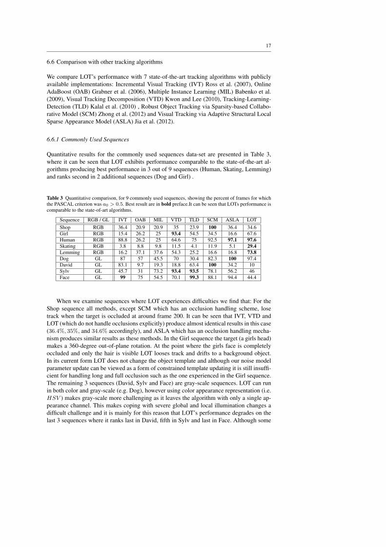
Quantitative results for the commonly used sequences data-set are presented in Table 3,where it can be seen that LOT exhibits performance comparable to the state-of-the-art al-gorithms producing best performance in 3 out of 9 sequences (Human, Skating, Lemming)and ranks second in 2 additional sequences (Dog and Girl) .

Table 3 Quantitative comparison, for 9 commonly used sequences, showing the percent of frames for whichthe PASCAL criterion was a0 > 0.5. Best result are in bold preface.It can be seen that LOTs performance iscomparable to the state-of-art algorithms.

Sequence RGB / GL IVT OAB MIL VTD TLD SCM ASLA LOTShop RGB 36.4 20.9 20.9 35 23.9 100 36.4 34.6Girl RGB 15.4 26.2 25 93.4 54.5 34.5 16.6 67.6Human RGB 88.8 26.2 25 64.6 75 92.5 97.1 97.6Skating RGB 3.8 8.8 9.8 11.5 4.1 11.9 5.1 29.4Lemming RGB 16.2 37.1 37.6 54.3 25.2 16.6 16.8 73.8Dog GL 87 57 45.5 70 30.4 82.3 100 97.4David GL 83.1 9.7 19.3 18.8 63.4 100 34.2 10Sylv GL 45.7 31 73.2 93.4 93.5 78.1 56.2 46Face GL 99 75 54.5 70.1 99.3 88.1 94.4 44.4

When we examine sequences where LOT experiences difficulties we find that: For theShop sequence all methods, except SCM which has an occlusion handling scheme, losetrack when the target is occluded at around frame 200. It can be seen that IVT, VTD andLOT (which do not handle occlusions explicitly) produce almost identical results in this case(36.4%, 35%, and 34.6% accordingly), and ASLA which has an occlusion handling mecha-nism produces similar results as these methods. In the Girl sequence the target (a girls head)makes a 360-degree out-of-plane rotation. At the point where the girls face is completelyoccluded and only the hair is visible LOT looses track and drifts to a background object.In its current form LOT does not change the object template and although our noise modelparameter update can be viewed as a form of constrained template updating it is still insuffi-cient for handling long and full occlusion such as the one experienced in the Girl sequence.The remaining 3 sequences (David, Sylv and Face) are gray-scale sequences. LOT can runin both color and gray-scale (e.g. Dog), however using color appearance representation (i.e.HSV ) makes gray-scale more challenging as it leaves the algorithm with only a single ap-pearance channel. This makes coping with severe global and local illumination changes adifficult challenge and it is mainly for this reason that LOT’s performance degrades on thelast 3 sequences where it ranks last in David, fifth in Sylv and last in Face. Although some

18




Fig. 5 Sample frames from three sequences: Dog, Skating and Lemming. The different algorithms are: IVTin Yellow, OAB in Cyan, MIL in Red, VTD in Magenta and LOT in light Green.

methods produce better results for some sequences, looking at the entire dataset it can beseen that the overall performance of LOT is comparable to the state-of-the-art methods.We believe that MIL and OAB have poorer performance mainly due to their lack of scaleadaptability.

Figure 5 presents sample frames from 3 sequences (Dog, Skating and Lemming) qual-itatively showing LOT’s ability to cope with difficult appearance changes such as massivescale changes and out-of-plane-rotations.

6.6.2 New Sequences

LOT was also compared to the state-of-the-art algorithms using our second data-set of 6challenging new sequences. Sample frames from these sequences are presented in Figure 6.

The first, 481 frame long, sequence shows a Down-Hill (DH) bike ride. As the riderjumps and moves in and out of shade a lot of motion blur, deformations and illuminationchanges are created. IVT, TLD and SCM drift after the first jump at around frame 56, MILand OAB keep tracking until around frame 400 where they also drift. Only VTD and LOTare able to track the rider until the end of the sequence.

The second, 951 frame long, sequence we captured is of a T-shirt undergoing severenon-rigid deformations and motion blur. LOT with its inherent ability to explain non-rigiddeformations is able to track the shirt throughout the entire length of the sequence. LOToutperforms all other methods except ASLA which is able to produce more accurate results.

The third, 900 frame long, sequence was taken from the PETS-2006 dataset1. It shows aman walking around a busy train station making many pose changes and undergoing severalocclusions. Although LOT does not have an explicit mechanism for handling occlusions itis able to handle partial occlusions by tracking the remaining visible part of the target whichoften captures the full target color statistics. In this sequence the first partial occlusion occursaround frame 35 causing IVT, OAB, TLD, ASLA and MIL to drift. A second occlusion at

1 http://www.cvg.rdg.ac.uk/PETS2006/data.html

19

Table 4 Quantitative comparison, for 6 new sequences, showing the percent of frames for which the PASCALcriterion was a0 > 0.5. Best result are in bold preface. LOT has the best overall performance on this dataset.

Sequence RGB / GL IVT OAB MIL VTD TLD SCM ASLA LOTDH RGB 8.9 47.8 45.5 69.4 10.8 8.3 8.7 92.3Shirt RGB 0.5 66.7 32.5 79 0.6 80.8 92.4 88.1Train RBG 2.7 3.4 2.3 2.9 2.8 10 4.6 69.6UCSDPeds GL 26.4 42.5 26.8 60.5 55.6 100 99.2 73.9Boxing RGB 7.3 18.7 18.4 21.2 28.8 34.8 55.2 70.1Towel RGB 8.8 5 46 34.5 94.7 90.1 44 99.7

around frame 60 throws VTD and SCM off track as well. LOT is able to overcome these 2occlusion by shrinking and matching to the remaining visible part of the target. It continuestracking the man for the entire length of the sequence while overcoming pose changes andadditional occlusions. We note that the final tracking score for this sequence is only 69.7%

since during the occlusions the predicted bounding box shrinks to the visible part of thetarget while the ground truth annotation continues marking the whole occluded target.

The forth, 261 frame long, gray-scale, sequence taken from the UCSD crowd dataset2

shows two people walking and fighting. We track both people as a single target. This crowdtarget undergoes non-rigid deformations as the people draw nearer and apart and as theyfight with each other. All the methods are able to track the targets location throughout mostof the sequence with only minor glitches, LOT ranks in 3rd place producing results betterthan most trackers and second only to SCM and ASLA.

The fifth, 352 frame long, is a boxing sequence. At the beginning of this sequence onlyLOT is able to correctly track the boxer through the difficult pose changes. All methods driftbetween frame 200-225 due to a rapid movement followed by a full occlusion however LOTis able to lock back on at frame 261 and continue tracking the target until the end of thesequence.

The sixth and last, 374 frame long, sequence (taken from Alterman et al. (2012)) wasshot from underwater into air. Our target is a towel hanging on a fence. This target is subjectto a complex non-uniform deformation field caused by the waters movement. Due to theinherent properties of LOT it is able to handle these difficult deformations and producenearly perfect tracking. TLD and SCM also produce good results for this sequence but notas good as LOT. Other algorithms drift.

Quantitative results are presented in Table 4. LOT has the best overall performance, itoutperforms the other tracking methods producing better results for all but one sequence(where it comes second).

7 Conclusions

Locally Orderless Tracking is a new visual tracking algorithm that estimates and adapts,on-line, to the rigidity of the tracked object. The algorithm is governed by a small set ofparameters Θ that are estimated on-line allowing it to go from rigid template matching onone end to histogram-like tracking on the other, or be anywhere in between. At the heartof this framework lies Locally Orderless Matching, a new probabilistic interpretation ofEMD that rigorously shows how EMD can be used to infer the likelihood that patch P is anoisy replica of patch Q using some noise model with parameters Θ. Since the framework

2 http://www.svcl.ucsd.edu/projects/peoplecnt/index.htm

20







Fig. 6 Sample frames from the new sequence set: DH, Shirt, Train, UCSDPeds, Boxing and Towel. Thedifferent algorithms are: IVT in Yellow, OAB in Cyan, MIL in Red, VTD in Magenta and LOT in lightGreen.

is generic any noise model can be plugged in and we have demonstrated the use of twosuch noise models. We have shown the significance and importance of estimating noisemodel parameters on-line and demonstrated how this parameter estimation and adaptationcan be achieved using the data at hand both theoretically and empirically. Finally we haveshown that LOT’s performance is comparable to state-of-the-art methods on a wide range ofcommonly used and new videos presenting superior performance in many cases.

Future work is intended in 3 main aspects: The first is exploiting the flow produced dur-ing the EMD calculation not merely for parameter update but also for on-line template up-date and foreground-background target segmentation which can help in overcoming occlu-sions. The second aspect is speed where we believe that using different Superpixel schemesand maybe some EMD approximations can make this algorithm run at real-time. The third

21

aspect is looking into different noise models and appearance representations that might bebetter suited for specific applications (such as tracking in gray-scale sequences).

A Additional noise models

A.1 Uniform Noise

A Uniform distribution with parameter r can be used as location and/or appearance noise model again. Dueto the independence assumed between appearance and location parameters p, q, r,D will be used without thesuperscripts A,L.

Pr(p|q, r) ={

1(2r)D

||p− q||∞ ≤ r0 otherwise

(20)

Where D is the dimension of p and q. The ground distance in this case is:

d(p, q) =

{D · log(2r) ||p− q||∞ ≤ r∞ otherwise (21)

This distance means the cost of changing the appearance and/or location of a pixel by less than a certain quantcosts nothing (the same as not moving it at all), and changing it by more than that is not allowed.

This model may pose some problems as certain mismatches are not allowed at all and also since thesignature EMD problem can become unfeasible in some cases i.e. giving∞ distance. Therefore a mixture oftwo uniforms might be a better choice.

A.2 Uniform-Mixture Noise

Using a mixture of two uniforms provides us with one low cost for small perturbations and a second highcost (but not ∞) for large ones.This means we allow any match but with high cost. The parameter for thesecond uniform should include the entire space. We formulate this model using a mixture variable h ∼Bernoulli(α) and marginalizing over it:

Pr(p|q, r, α) = αPr(p|q, h = 0) + (1− α)Pr(p|q, h = 1) (22)

Where P (p|q, h = {0, 1}) are both uniform distributions. The ground distance is given by:

d(p, q) =

{−log( α

(2r)D+ 1−α

S) ||p− q||∞ ≤ r

−log( 1−αS

) otherwise(23)

Where S is the hyper-volume of the entire space (e.g. for un-normalized RGB space S = (28)3 which is theRGB cube volume).

A.2.1 Uniform-Mixture Parameter Estimation

This model has two parameters Θ = {α, r}. We use the EMD correspondence mapping fij and the grounddistance matrix dij = d(pi, qj) from which we build a CDF of the transported distance. We denoted thisCDF by c(r) : [0, R] → [0, 1] where R is the maximal distance a mass can move in our subspace i.e.

∀r c(r) =

∑i,j:dij≤r

fij dij∑i,jfij dij

. We can now estimate α and r using an ML consideration:

logPr(P |Q, r, α) =∑ilogPr(pi|qj) =

∑i∈D1

log( α(2r)D

+ 1−αS

) +∑i∈D2

log( 1−αS

) =

N [c(r) · log( α(2r)D

+ 1−αS

) + (1− c(r)) · log( 1−αS

)](24)

22

where D1 = {i : ||pi − qj ||∞ ≤ r}, D2 = {i : ||pi − qj ||∞ > r} and N is the total mass. If we onlywant to estimate r and leave α constant we can numerically find r that maximizes (24). For estimating bothr and α we differentiate (24) with respect to α and compare to 0 which leads to:

α =c(r)S − (2r)D

S − (2r)D(25)

Plugging this result back to equation (24) we see that we need to find:

argmaxr

(c(r) · log(

c(r)

(2r)D) + (1− c(r)) · log(

1− c(r)S − (2r)D

)

)(26)

Equation (26) can be solved numerically given c(r) built using the EMD result and then α is calculated basedon equation (25).

B Proof of Proposition 2

Proof For all i, j in (7), we take all the variables {fk1j , . . . , fkwpij} that correspond to wpi similar pixels

(with singleton weights). We then collapse each set into a single variable representing their sum gij =∑wpi

l=1 fklj . This can be done as their coefficients (dklj ) in the optimization argument∑ijfijdij are the

same. Thus the wpi constraints of the form∑j fklj = 1 can be replaced with a single constraint demanding∑

j gij = wpi and the wqj constraints of the form∑i fikl = 1 can be replaced with a single constraint

demanding∑i gij = wqj . We then obtain the following integer linear program (ILP):

minn1∑i=1

n2∑j=1

gijdij

such thatn1∑i=1

gij = wpi ,n2∑j=1

gij = wqj , gij ∈ {0, 1, . . . ,min(wpi , wqj )}

(27)

By construction we have that the space of feasible solutions w.r.t to optimization problem (7) did not change

i.e. minm∑i=1

m∑j=1

fijdij = minn1∑i=1

n2∑j=1

gijdij where the dij on the left and right side of the equation are set

according to the appropriate source and sink nodes. Again this is true since every gij is simply a sum of fijhaving the same ground distance dij . If we now write (27) in the canonical form (as we did in proposition 1)we see that the matrix A is again totally unimodular which means that the relaxed linear programming (LP)problem has an integral solution. This relaxed LP is exactly optimization problem (8) and given a solution(i.e. the gij ) to this problem we can always find an assignment to the fij such that would satisfy (7). This istrue since we can always break down the compact signatures back into the pixel-wise problem with singletonbins which as we have shown would have the same minima. ut

C Proof of Proposition 3

Proof It is enough to look at a single step of uniting two clusters. Assume we unite pn1 , pn1−1 into a singlecluster pn−1. For weight/flow assignment fij we have:

n1∑i=1

n2∑j=1

fijdij =

n1−2∑i=1

n2∑j=1

fijdij +

n2∑j=1

fn−1,jd(pn1−1, qj) + fn1,jd(pn1 , qj) (28)

23

Denoting C =n1−2∑i=1

n2∑j=1

fijdij and using the triangle inequality we have:

C +n2∑j=1

fn−1,jd(pn1−1, qj) + fn1,jd(pn1 , qj)

≤ C +n2∑j=1

fn1−1,j [d(pn1−1, pn1−1) + d(pn1−1, qj)] + fn,j [d(pn1 , pn1−1) + d(pn1−1, qj)]

(29)Reorganizing the last expression by collecting elements related to the distance between the original clusters

and their crude version and elements related to the distance between the crude cluster and its assignment leadsto,

C +n2∑j=1

(fn1−1,j + fnj)d(pn1−1, qj) + wn1−1d(pn1−1, pn1−1) + wn1d(pn1 , pn1−1)

= C +n2∑j=1

fn1−1,jd(pn1−1, qj) + wn1−1d(pn1−1, pn1−1) + wn1d(pn1 , pn1−1)(30)

Where fn1−1 = fn1−1+fn1 . The expressionn1−2∑i=1

n2∑j=1

fijdij+n2∑j=1

fn1−1,jd(pn1−1, qj) appearing

in the last line is the optimization argument EMD(P , Q, d). Lets fix now the variables {fij}n−2i=1 , fn1−1

to the argmin values of the problem (the values achieving the minimun for EMD(P , Q, d). Now using theinequality in (30) we have

EMD(P , Q, d) =n1−2∑i=1

n2∑j=1

fijdij +n2∑j=1

fn1−1,jd(pn1−1, qj)

≥n1∑i=1

n2∑j=1

fijdij − wn1−1d(pn1−1, pn1−1)− wnd(pn1 , pn1−1)

≥ argminfij

n1∑i=1

n2∑j=1

fijdij − wn1−1d(pn1−1, pn1−1)− wnd(pn1 , pn1−1)

= EMD(P,Q, d)− wn1−1d(pn1−1, pn1−1)− wnd(pn1 , pn1−1)

(31)

Since wn1−1d(pn1−1, pn1−1) + wnd(pn1 , pn1−1 > 0 it follows that,

|EMD(P,Q, d)− EMD(P , Q, d)| ≥ wn1−1d(pn1−1, pn1−1) + wn1d(pn1 , pn1−1) (32)

In an analogous way it can be shown that,

|EMD(P,Q, d)− EMD(P, Q, d)| ≥ wn2−1d(qn2−1, qn2−1) + wn2d(qn2 , qn2−1) (33)

The proposition follows by repeating this argument for all pi, qj

References

M. Alterman, Y. Schechner, P. Perona, J. Shamir, Independent components in dynamic refraction. CCITReport 805 (2012)

S. Avidan, Ensemble Tracking, in CVPR, 2005, pp. 494–501B. Babenko, M.H. Yang, S. Belongie, Visual Tracking with Online Multiple Instance Learning, in CVPR,

2009S. Boltz, F. Nielsen, S. Soatto, Earth Mover Distance on Superpixels, in ICIP, 2010D. Comaniciu, Bayesian Kernel Tracking., in DAGM-Symposium, 2002, pp. 438–445A. Doucet, N. de Freitas, N. Gordon, Sequential monte carlo methods in practice. Springer-Verlag (2001)A. Elgammal, R. Duraiswami, L.S. Davis, Probabilistic Tracking in Joint Feature-spatial Spaces, in CVPR,

2003M. Everingham, L.J. Van Gool, C.K.I. Williams, J.M. Winn, A. Zisserman, The pascal visual object classes

(voc) challenge. IJCV (2010)B.V. Ginneken, B.M.T. Haar Romeny, Applications of Locally Orderless Images, in Scale-Space Theories in

Computer Vision, 1999

24

M. Godec, P.M. Roth, H. Bischof, Hough-based Tracking of Non-rigid Objects, in ICCV, 2011H. Grabner, M. Grabner, H. Bischof, Real-time Tracking Via Online Boosting, in BMVC, 2006G.D. Hager, P.N. Belhumeur, Efficient region tracking with parametric models of geometry and illumination.

PAMI (1998)X. He, R. Zemel, D. Ray, Learning and Incorporating Top-down Cues in Image Segmentation, in ECCV,

2006I. Heller, C.B.G. Tompkins, An extension of a theorem of dantzig’s. Linear Inequalities and Related Systems,

Annals of Mathematics Studies, 38, Princeton (NJ), 247–254 (1956)D. Hoiem, A. Efros, M. Hebert, Geometric Context from a Single Image, in ICCV, 2005M. Isard, A. Blake, Condensation - conditional density propagation for visual tracking. IJCV (1998)X. Jia, H. Lu, M.H. Yang, Visual Tracking Via Adaptive Structural Local Sparse Appearance Model, 2012Z. Kalal, K. Mikolajczyk, J. Matas, Tracking-learning-detection. TPAMI (2010)J.J. Koenderink, A.J. Van Doorn, The structure of locally orderless images. IJCV (1999)J. Kwon, K.M. Lee, Visual Tracking Decomposition, in CVPR, 2010E. Levina, P. Bickel, The Earth Mover’s Distance Is the Mallows Distance: Some Insights from Statistics, in

ICCV, 2001A. Levinshtein, A. Stere, K.N. Kutulakos, D.J. Fleet, S.J. Dickinson, K. Siddiqi, Turbopixels: Fast superpixels

using geometric flows. TPAMI (2009)X. Mei, H. Ling, Y. Wu, E. Blasch, L. Bai, Minimum Error Bounded Efficient L1 Tracker with Occlusion

Detection, in ICCV, 2011S. Oron, A. Bar-Hillel, D. Levi, S. Avidan, Locally Orderless Tracking, in CVPR, 2012S. Peleg, M. Werman, H. Rom, A unified approach to the change of resolution: Space and gray-level. TPAMI

(1989)X. Ren, J. Malik, Learning a Classification Model for Segmentation, in ICCV, 2003D. Ross, J. Lim, M.H. Yang, Adaptive Probabilistic Visual Tracking with Incremental Subspace Update, in

ECCV, 2004D. Ross, J. Lim, R.S. Lin, M.H. Yang, Incremental learning for robust visual tracking. IJCV (2007)Y. Rubner, C. Tomasi, L.J. Guibas, The earth mover’s distance as a metric for image retrieval. IJCV (2000)J. Santner, C. Leistner, A. Saffari, T. Pock, H. Bischof, Prost:parallel Robust Online Simple Tracking, in

CVPR, 2010S. Wang, H. Lu, F. Yang, M.H. Yang, Superpixel Tracking, in ICCV, 2011A. Yilmaz, O. Javed, M. Shah, Object tracking: A survey. ACM Comput. Surv. (2006)Q. Zhao, Z. Yang, H. Tao, Differential earth mover’s distance with its applications to visual tracking. PAMI

(2010)W. Zhong, H. Lu, M.H. Yang, Robust Object Tracking Via Sparsity-based Collaborative Model, in CVPR,

2012

locally orderless tracking - tau

Documents