localization in wireless sensor networks haroon...
TRANSCRIPT
Localization
inWireless Sensor Networks
Haroon Rashid
Department of Computer Science and Engineering
National Institute of Technology Rourkela
Rourkela-769 008, Odisha, India
July, 2013

Localizationin
Wireless Sensor Networks
Thesis submitted in partial fulfillment
of the requirements for the degree of
Master of Technology
(Research)
in
Computer Science and Engineering
by
Haroon Rashid
(Roll No: 611CS102)
under the guidance of
Dr. Ashok Kumar Turuk
Department of Computer Science and Engineering
National Institute of Technology Rourkela
Rourkela-769 008, Odisha, India
July, 2013
Department of Computer Science and Engineering
National Institute of Technology Rourkela
Rourkela-769 008, Odisha, India.
July 20, 2013
Certificate
This is to certify that the work in the thesis entitled “Localization in Wireless Sensor
Networks” by Haroon Rashid is a record of an original research work carried out under
my supervision and guidance in partial fulfillment of the requirements for the award of the
degree of Master of Technology (Research) in Computer Science and Engineering, National
Institute of Technology, Rourkela. Neither this thesis nor any part of it has been submitted
for any degree or academic award elsewhere.
Dr. Ashok Kumar Turuk
Associate Professor
CSE department of NIT Rourkela
Acknowledgement
First of all, I am very thankful to Almighty Allah for granting me the wisdom, health and
strength for doing this work. Next, I am thankful to my supervisor Prof. Ashok Kumar
Turuk for providing me an opportunity to work under him. I am indebted to him for being
a constant source of knowledge for me from joining of this course till now. He not only
corrected me in the technical issues related to the localization of wireless sensor networks,
but his painstakingly paper correction as well as paper presentation helped me a lot to
represent this research work in a novel way.
I owe a deep gratitude to Prof. S. K. Rath, Prof. B. Majhi, Prof. S. K. Patra, and
Prof. S. Das for not only being the members of my Masters Scrutiny Committee, but also
providing insightful comments at different times during these two years.
I am also thankful to my lab-mates Alekha Kumar Mishra, Yogender Soni, Ambuj
Kumar, and Rajendra Prasad for maintaining a calm research oriented environment in the
lab. Also, they were source of continuous technical discussions.
At last, I would like to say that all this would have been difficult to achieve without the
support and patience of my parents. They have been a source of consistent motivation for
this work. I love them for their perseverance and the moral character they provided to me.
Haroon Rashid
Abstract
The technique of finding physical co-ordinates of a node is known as localization. Importance
of localization arises from the need to tag the sensed data and associate events with their
location of occurrence. Location information of a sensor node can be obtained by using GPS.
But, installing GPS in every node is not a feasible solution. This is because: (i) sensor nodes
are deployed in a very large number. Installing GPS at every node will increase the cost
as well as size, (ii) GPS consume power, which will effect the network lifetime. Moreover,
location cannot be pre-programmed as it is un-known where nodes will be deployed during
their operational phase.
In this thesis, we have made an attempt to address localization in static as well as
mobile sensor networks. For static network we have proposed two distributed range based
localization techniques called (i) Localization using a single anchor node (LUSA), (ii) Dis-
tributed binary node localization estimation (DBNLE). Both the techniques are proposed
for grid environment. In LUSA, we have identified three types of node: anchor, special and
unknown node. For every anchor node there exists two special node and they are placed
perpendicular to the anchor node. Localization in LUSA is achieved by a single anchor node
and two special nodes. Localization occurs in two steps. First special nodes are localized
and then the unknown nodes. We have compared LUSA with a closely related localization
technique called Multi-duolateration (MDL). It is observed that the localization error and
localization time is lesser in LUSA. In DBNLE a node is localized with only two location
aware nodes instead of three nodes in most localization techniques. This not only reduces
the localization time but also the dependency.
For mobile WSNs, we have proposed a distributed localization technique called dead
reckoning localization in mobile sensor networks (DRLMSN). In DRLMSN, localization is
done at discrete time intervals called checkpoint. Unknown nodes are localized for the first
time using three anchor nodes. In their subsequent localization, only two anchor nodes
are used. Using Bezouts theorem, we estimate two possible locations of a node. A dead
reckoning approach is used to select one among the two estimated locations. We have used
Castalia simulator to evaluate the performance of the schemes.
Dissemination of Work
Published:
1. H. Rashid, A. K. Turuk, “Localization of Wireless Sensor Networks Using a Single
Anchor Node”, Wireless Personal communications (Springer), 72(2), 2013.
Under Review:
1. H. Rashid, A. K. Turuk, “Distributed Binary Node Localization Estimation Ap-
proach”, International Journal of Sensor Networks (Inderscience), 2013.
2. H. Rashid, A. K. Turuk, “Dead Reckoning Localization Technique for Mobile Wire-
less Sensor Networks”, IET Wireless Sensor Systems, 2013. [Accepted With Revi-
sion]
v
Contents
Certificate ii
Acknowledgement iii
Abstract iv
Dissemination of Work v
List of Figures viii
List of Tables x
1 Introduction 1
1.1 Key Issues in Wireless Sensor Networks . . . . . . . . . . . . . . . . . . . . . 2
1.2 Motivation . . . . . . . . . . . . . . . . . . . . . . . . . . . . . . . . . . . . . 4
1.3 Objective . . . . . . . . . . . . . . . . . . . . . . . . . . . . . . . . . . . . . . 5
1.4 Organization of The Thesis . . . . . . . . . . . . . . . . . . . . . . . . . . . . 5
2 Localization System 7
2.1 Distance/Angle Estimation . . . . . . . . . . . . . . . . . . . . . . . . . . . . 7
2.1.1 Time of Arrival . . . . . . . . . . . . . . . . . . . . . . . . . . . . . . . 8
2.1.2 Time-Difference of Arrival . . . . . . . . . . . . . . . . . . . . . . . . . 9
2.1.3 Received Signal Strength Indication . . . . . . . . . . . . . . . . . . . 9
2.1.4 Angle/Direction of Arrival . . . . . . . . . . . . . . . . . . . . . . . . . 11
2.1.5 Hop Count . . . . . . . . . . . . . . . . . . . . . . . . . . . . . . . . . 12
2.2 Position Calculation . . . . . . . . . . . . . . . . . . . . . . . . . . . . . . . . 13
2.2.1 Trilateration/Multilateration . . . . . . . . . . . . . . . . . . . . . . . 14
2.2.2 Triangulation . . . . . . . . . . . . . . . . . . . . . . . . . . . . . . . . 15
2.3 Localization algorithm . . . . . . . . . . . . . . . . . . . . . . . . . . . . . . . 15
vi

2.4 Summary . . . . . . . . . . . . . . . . . . . . . . . . . . . . . . . . . . . . . . 20
3 Localization Using Single Anchor Node 21
3.1 Proposed Technique . . . . . . . . . . . . . . . . . . . . . . . . . . . . . . . . 21
3.2 Simulation Results . . . . . . . . . . . . . . . . . . . . . . . . . . . . . . . . . 23
3.2.1 Localization Error . . . . . . . . . . . . . . . . . . . . . . . . . . . . . 26
3.2.2 Localization Time . . . . . . . . . . . . . . . . . . . . . . . . . . . . . 28
3.3 Summary . . . . . . . . . . . . . . . . . . . . . . . . . . . . . . . . . . . . . . 28
4 Distributed Binary Estimation Approach 30
4.1 Introduction . . . . . . . . . . . . . . . . . . . . . . . . . . . . . . . . . . . . . 30
4.2 Distributed Binary Node Localization . . . . . . . . . . . . . . . . . . . . . . 30
4.2.1 Localization of Edge nodes . . . . . . . . . . . . . . . . . . . . . . . . 31
4.2.2 Localization of Unknown nodes . . . . . . . . . . . . . . . . . . . . . . 33
4.3 Simulation Results . . . . . . . . . . . . . . . . . . . . . . . . . . . . . . . . . 36
4.3.1 Localization Error . . . . . . . . . . . . . . . . . . . . . . . . . . . . . 37
4.3.2 Localization Time . . . . . . . . . . . . . . . . . . . . . . . . . . . . . 37
4.4 Summary . . . . . . . . . . . . . . . . . . . . . . . . . . . . . . . . . . . . . . 38
5 Dead Reckoning Technique 39
5.1 Introduction . . . . . . . . . . . . . . . . . . . . . . . . . . . . . . . . . . . . . 39
5.2 Related work . . . . . . . . . . . . . . . . . . . . . . . . . . . . . . . . . . . . 40
5.3 Proposed Localization Technique . . . . . . . . . . . . . . . . . . . . . . . . . 42
5.3.1 Initialization Phase: . . . . . . . . . . . . . . . . . . . . . . . . . . . . 43
5.3.2 Sequent Phase: . . . . . . . . . . . . . . . . . . . . . . . . . . . . . . . 43
5.4 Performance Evaluation . . . . . . . . . . . . . . . . . . . . . . . . . . . . . . 49
5.5 Summary . . . . . . . . . . . . . . . . . . . . . . . . . . . . . . . . . . . . . . 53
6 Conclusions 55
6.1 Contribution . . . . . . . . . . . . . . . . . . . . . . . . . . . . . . . . . . . . 55
6.2 Direction for Future Research . . . . . . . . . . . . . . . . . . . . . . . . . . . 56

List of Figures
1.1 Wireless Sensor Network. . . . . . . . . . . . . . . . . . . . . . . . . . . . . . 1
1.2 Protocol stack of wireless sensor network. . . . . . . . . . . . . . . . . . . . . 2
2.1 Three components of localization system. . . . . . . . . . . . . . . . . . . . . 7
2.2 (a) ToA, (b) ToA using RTT, (c) TDoA . . . . . . . . . . . . . . . . . . . . . 8
2.3 Effect of path loss exponent on RSSI with distance. . . . . . . . . . . . . . . . 11
2.4 Angle of Arrival. . . . . . . . . . . . . . . . . . . . . . . . . . . . . . . . . . . 12
2.5 Distance estimation using hop count. . . . . . . . . . . . . . . . . . . . . . . . 13
2.6 Trilateration . . . . . . . . . . . . . . . . . . . . . . . . . . . . . . . . . . . . 13
2.7 Triangulation . . . . . . . . . . . . . . . . . . . . . . . . . . . . . . . . . . . . 13
3.1 Deployment of Beacon node, Special node and Unknown node in a grid. . . . 22
3.2 Localization in LUSA. . . . . . . . . . . . . . . . . . . . . . . . . . . . . . . . 22
3.3 Localization pattern. . . . . . . . . . . . . . . . . . . . . . . . . . . . . . . . . 23
3.4 Beacon node at the corner of grid. . . . . . . . . . . . . . . . . . . . . . . . . 24
3.5 Beacon node at the middle of grid. . . . . . . . . . . . . . . . . . . . . . . . . 24
3.6 Process of localization when the beacon node is placed at the middle of the
grid. . . . . . . . . . . . . . . . . . . . . . . . . . . . . . . . . . . . . . . . . . 24
3.7 Distribution of localization error without interference in LUSA and MDL. . . 25
3.8 Mean localization error (meters) in various grid: (a) Without interference,
(b) With interference. . . . . . . . . . . . . . . . . . . . . . . . . . . . . . . . 26
3.9 Distribution of localization error with interference in LUSA and MDL. . . . . 27
3.10 Localization Time. . . . . . . . . . . . . . . . . . . . . . . . . . . . . . . . . . 28
4.1 Deployment of nodes in a grid, showing the placement of anchor and unknown
nodes. . . . . . . . . . . . . . . . . . . . . . . . . . . . . . . . . . . . . . . . . 31
4.2 Selection of settled nodes for localization. . . . . . . . . . . . . . . . . . . . . 33
4.3 Localization of unknown nodes 7 and 10 . . . . . . . . . . . . . . . . . . . . . 34
viii

4.4 Nodes involved in the localization of unknown nodes in a 4 x 4 grid. . . . . . 34
4.5 Localization pattern in a 4 x 4 grid. . . . . . . . . . . . . . . . . . . . . . . . 35
4.6 Localization process in MDL: (a) Localization of edge nodes, (b) Localization
of surface nodes using nearest edge nodes. . . . . . . . . . . . . . . . . . . . . 35
4.7 Geographical distribution of error for a grid size of 6 × 4, 6 × 6, and 9 × 9
is shown in a, c, and e respectively for MDL and b, d, and f respectively for
DBNLE. . . . . . . . . . . . . . . . . . . . . . . . . . . . . . . . . . . . . . . . 36
4.8 Localization time of MDL vs. DBNLE in different grid sizes. . . . . . . . . . 38
5.1 Initialization phase: (a) At the first checkpoint, anchor nodes transmit bea-
cons and normal nodes localize via trilateration; (b) normal nodes that are
short of 1 or 2 beacons localize with the help of settled nodes. . . . . . . . . 45
5.2 Normal node 3 at checkpoint ti+1 estimate two locations P1 and P2 using two
anchor nodes 0 and 2. The correct position is selected by using the previous
position of node 3 at checkpoint ti . . . . . . . . . . . . . . . . . . . . . . . . . 46
5.3 Impact of increase in the number of nodes on the localization error in modified
random waypoint mobility model. . . . . . . . . . . . . . . . . . . . . . . . . . 50
5.4 Impact of increase in the number of nodes on the localization error in random
direction mobility model. . . . . . . . . . . . . . . . . . . . . . . . . . . . . . 50
5.5 Mobility pattern of nodes in random waypoint mobility model. . . . . . . . . 50
5.6 Mobility pattern of nodes in random direction mobility model. . . . . . . . . 50
5.7 Impact of increase in anchors on the localization error in modified random
waypoint mobility model. . . . . . . . . . . . . . . . . . . . . . . . . . . . . . 51
5.8 Impact of increase in anchors on the localization error in random direction
mobility model. . . . . . . . . . . . . . . . . . . . . . . . . . . . . . . . . . . . 51
5.9 Impact of node deployment on the localization error in modified random
waypoint mobility model. . . . . . . . . . . . . . . . . . . . . . . . . . . . . . 53
5.10 Impact of node deployment on the localization error in random direction
mobility model. . . . . . . . . . . . . . . . . . . . . . . . . . . . . . . . . . . . 53
5.11 Percenatge of localized nodes at successive checkpoints in modified random
waypoint mobility model. . . . . . . . . . . . . . . . . . . . . . . . . . . . . . 54
5.12 Percenatge of localized nodes at successive checkpoints in random direction
mobility model. . . . . . . . . . . . . . . . . . . . . . . . . . . . . . . . . . . . 54
List of Tables
2.1 A qualitative comparison of range based localization techniques. . . . . . . . 12
3.1 Evaluation of proposed algorithm, placing the beacon node at two different
places within the network. . . . . . . . . . . . . . . . . . . . . . . . . . . . . . 24
5.1 Comparison of different localization techniques for Mobile WSN’s . . . . . . . 42
x

Chapter 1
Introduction
Wireless Sensor Networks (WSNs) has become an emerging area of interest among the
academia and industry in the last one decade [1]. It consists of a large number of densely
deployed nodes which are tiny, low power, in-expensive, multi-functional and have limited
computational and communication capabilities. These nodes interact with their environ-
ment, sense the parameters of the interest such as temperature, light, sound, humidity, and
pressure; and report it to the sink node/base station. Deployment of WSN may vary from
a controlled indoor environment to a remote and inaccessible area. Therefore, a sensor
node is configured with necessary extra components for on-board limited processing ability,
communication, and storage capabilities. A typical WSN is shown in Figure - 1.1.
���������
���������
���������
���������
������������
������������
������������
������������
���������
���������
��������
��������
������������
������������
���������
���������
���������
���������
Event occurs
Monitoring System
Forwarding node
Sink node
Gateway
Internet
2. Event detection and reporting 3. Event processing1. Event occurrence
������������������
Figure 1.1: Wireless Sensor Network.
With the span of time, usage of WSN in diverse field have increased with the agile growth
in micro-electromechanical systems (MEMS), very large scale integration (VLSI), low-power
radios, and wireless communication protocols. Applications of WSN includes environment
monitoring (e.g., habitat, geophysical monitoring) [2–4], traffic management [5], military
applications (e.g., surveillance and battle field monitoring) [6], health monitoring (e.g.,
1

Chapter 1 Introduction
medical sensing) [7, 8], industrial process control, context-aware computing (e.g., smart
homes, remote metering), infrastructure protection (e.g., bridges, tunnels) [9] and so on.
For interoperability, sensor nodes produced by different manufacturer need to follow
a particular standard. Protocol stack of WSN consists of five layers: (i) physical layer,
(ii) data-link layer, (iii) network layer, (iv) transport layer, and (v) application layer [10].
Physical and data-link layer operations are specified by the task group 4 of IEEE 802.15,
accordingly named as IEEE 802.15.4. The remaining layers of WSN follow the ZigBee
standard, developed by the ZigBee Alliance, which consists of various companies working
for low-power, reliable and open global wireless networking standards focused on control,
monitoring, and sensor applications. An overview of protocol stack in WSNs and the main
functions performed at each layer is shown in Figure - 1.2.
32/64/128 bit−encryption
Star/ Mesh/ Cluster−Tree
PHY
MAC
Network
Security
API
Application
{{
Customer
Management Services (Synchronization)
ZigBee
Alliance
902 − 928 MHZ (North America)
20 kbps
Data rate
IEEE802.15.4
868 − 868.6 MHZ (Europe)
Band
2400 − 2483.5 MHZ (Worldwide) 250 kbps
40 kbps
Data Services.
Figure 1.2: Protocol stack of wireless sensor network.
1.1 Key Issues in Wireless Sensor Networks
Some of the important issues in WSNs are stated below:
(i) Energy Efficiency: Sensor nodes have limited battery capacity. This puts a con-
straint for other applications and on the lifetime of sensor node. Major sources of bat-
tery drainage include: (i) continuous sensing, (ii) transmission and reception modes
of radio. Therefore, to increase the lifetime in unattended environments, efficient al-
gorithms should be developed at each layer of WSN in concern with the less energy
utilization. This includes techniques of data compression, data fusion (removal of data
redundancy), rotation of cluster heads, and adaptive mechanisms for radio operations.
2

Chapter 1 Introduction
(ii) Routing: Topology of WSN changes too frequently; as new nodes are added or
some nodes die due to meager resources. Therefore, to increase the connectivity,
coverage, and remain updated of network topology, neighbour information should be
disseminated timely. Furthermore, transmitting node should identify the best reliable
shortest path to the sink node/base station. Therefore, routing serves as a bottleneck
in overall efficiency of WSN.
(iii) Time Synchronization: Synchronizing time in sensor nodes serves as a basic pre-
requisite for various applications and protocols such as Time division multiple access
(TDMA), Time difference of arrival (TDoA), Time of arrival (ToA) and so on. Basic
property of WSNs, i.e., co-operation in communication, computation, sensing and
actuation of different nodes solely depends on the time synchronization among nodes
[11].
(iv) Fault-Tolerance: Reliability in WSNs is oftenly affected by various faults arising
from environmental hazards, battery depletion, hardware malfunctioning and so on.
Individual node failures should not affect the global performance of WSNs. This rate of
failure may be high in harsh or hostile environments. In such cases, intended purpose
of WSN is achieved by techniques such as load balancing, etc. Nodes should have the
capability of self-testing, self-calibrating, self-recovering and so on [12].
(v) Localization: For robust WSN, localization of nodes is one of the most important
issue. Information sensed by a sensor node becomes useful only when its geographical
location is tagged. Geographical routing is possible only after the localization, and
other issues like spatial querying and load balancing can also be achieved [13].
(vi) Security: This is one of the critical issues in WSN deployments - where the purpose
is to get battle-field awareness or vigilance in confidential data monitoring systems.
In such cases, a node can be compromised at any layer if the security is not properly
implemented say:
(a) At application layer - to send the bogus data,
(b) At network layer - to change the routing information,
(c) At data-link layer - to schedule data transfer at inappropriate time slots resulting
in network jam.
3
Chapter 1 Introduction
In such cases, WSN should enable: (i) intrusion detection to prevent the integrity of
collected information, (ii) authentication system - to keep information privacy.
For smooth functioning of WSNs each issue needs deep investigation. Some of these issues
like synchronization, localization and data gathering needs much more attention. This is
because these not only help in attaining the basic function of WSNs but also serve as pre-
requisite for other applications. In this thesis, we have concentrated on the localization
issues in WSNs.
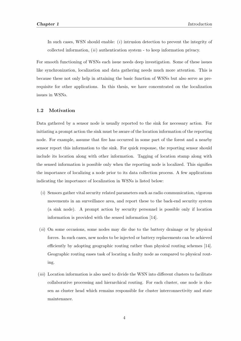
1.2 Motivation
Data gathered by a sensor node is usually reported to the sink for necessary action. For
initiating a prompt action the sink must be aware of the location information of the reporting
node. For example, assume that fire has occurred in some part of the forest and a nearby
sensor report this information to the sink. For quick response, the reporting sensor should
include its location along with other information. Tagging of location stamp along with
the sensed information is possible only when the reporting node is localized. This signifies
the importance of localizing a node prior to its data collection process. A few applications
indicating the importance of localization in WSNs is listed below:
(i) Sensors gather vital security related parameters such as radio communication, vigorous
movements in an surveillance area, and report these to the back-end security system
(a sink node). A prompt action by security personnel is possible only if location
information is provided with the sensed information [14].
(ii) On some occasions, some nodes may die due to the battery drainage or by physical
forces. In such cases, new nodes to be injected or battery replacements can be achieved
efficiently by adopting geographic routing rather than physical routing schemes [14].
Geographic routing eases task of locating a faulty node as compared to physical rout-
ing.
(iii) Location information is also used to divide the WSN into different clusters to facilitate
collaborative processing and hierarchical routing. For each cluster, one node is cho-
sen as cluster head which remains responsible for cluster interconnectivity and state
maintenance.
4

Chapter 1 Introduction
(iv) Sensor networks is like a distributed database for users to query the physical world for
useful information. With localization, efficient spatial querying by a sink or a gateway
node is responded only by the intended sensor node.
(v) Location based routing saves significant energy by eliminating the need for route
discovery and improve caching behaviour for applications where requests are location
dependent [15].
(vi) Determining the quality of coverage of all active sensors using their position.
1.3 Objective
Sensor nodes are low cost devices. Use of GPS to obtain location information will increase
their cost. An alternative to the use of GPS is to obtain location information through
localization algorithms. Use of localization algorithms mandate the deployment of a few
location aware node. The remaining nodes are localized with the help of these location
aware nodes. The objective of this thesis includes:
(i) Localization using lesser number of location-aware nodes.
(ii) Develop a localization algorithm with no extra hardware cost.
(iii) Reduce the localization error, and localization time.
1.4 Organization of The Thesis
The thesis is organized into following chapters:
Chapter 1: A brief introduction to wireless sensor networks is provided. Some of the key
issues in WSNs are identified. The importance of localization in WSNs is discussed.
Chapter 2: This chapter introduces the localization system. A brief review of different
localization schemes is presented.
Chapter 3: This chapter proposes a localization technique for grid environment. A single
anchor node is used for localization. The proposed technique is compared with a contem-
porary proposed for grid environment called multi-duolateration (MDL). We observed that
the proposed scheme has lesser localization time and error.
Chapter 4: In this chapter, we proposed a range based, distributed localization algorithm
for grid environment. We call the proposed scheme a Distributed Binary Node Localization
5

Chapter 1 Introduction
Estimation (DBNLE). It uses two reference/localized nodes for localization.
Chapter 5: This chapter proposes a localization technique called Dead Reckoning Local-
ization (DRLMSN) for mobile WSN. In this technique both the unknown and anchor nodes
are mobile. Through simulation, we have studied the impact of node mobility, anchor den-
sity, node density and deployment topology on location estimation.
Chapter 6: A few conclusions, along with the future scope for research in localization of
WSNs is mentioned in this chapter.
6
Chapter 2
Localization System
The objective of localization is to find the physical coordinates of sensor nodes. These
coordinates can be either global or relative. Localization is achieved with the help of a
few location aware nodes usually referred as seeds/anchor nodes/beacon nodes. These an-
chor nodes are either manually programmed with their physical position or use the global
positioning system (GPS) to determine their location.
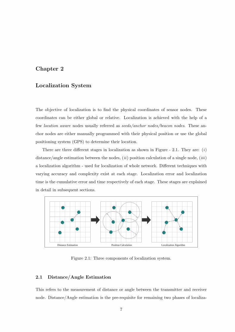
There are three different stages in localization as shown in Figure - 2.1. They are: (i)
distance/angle estimation between the nodes, (ii) position calculation of a single node, (iii)
a localization algorithm - used for localization of whole network. Different techniques with
varying accuracy and complexity exist at each stage. Localization error and localization
time is the cumulative error and time respectively of each stage. These stages are explained
in detail in subsequent sections.
��������
��������
���������
���������
������
������
������
������
��������
��������
��������
��������
������������
������������
������
������
���������
���������
���������
��������� ��
����
������
������������
������������
��������
��������
���������
���������
������
������
������
������ ���
������
���������
��������
��������
Distance Estimation Position Calculation Localization Algorithm
Figure 2.1: Three components of localization system.
2.1 Distance/Angle Estimation
This refers to the measurement of distance or angle between the transmitter and receiver
node. Distance/Angle estimation is the pre-requisite for remaining two phases of localiza-
7

Chapter 2 Localization System
tion. Different techniques for distance/angle estimation include: time of arrival (ToA), time
difference of arrival (TDoA), received signal strength indicator (RSSI), and angle of arrival
(AoA).
2.1.1 Time of Arrival
This technique estimates the distance by calculating the time required by a signal to traverse
from transmitter to receiver. Types of signal used includes: RF, acoustic, infrared and
ultrasound. GPS enabled devices use this technique for distance estimation.
������
������
������
������
������
������
������
������
������
������
������
������
���
���
������
������
������
������
������
������
Ultrasound Signal
BB
Del
ay
ta
tb
ta1
tb1
tb2
a2t
tb2
ta1
ta2
BAAA
(a) (b) (c)
Radio Signal tb1
Figure 2.2: (a) ToA, (b) ToA using RTT, (c) TDoA
We consider Figure - 2.2(a) to illustrate distance estimation using ToA. Let node A be
the sender and B the receiver, ta is the time at which a signal is transmitted from A and tb
be the time at which it is received at B, and v be the velocity of signal. Distance d between
A and B is estimated as:
d = (tb − ta)× v
Since, nodes are mostly not synchronized, distance between nodes at various instances as
calculated above may vary. Also, the signal (mostly ultrasound signals) speed may vary.
This is because they are oftenly affected by temperature, humidity and pressure. Therefore,
to remove the problem of synchronization ToA is reformed with round trip time (RTT).
This is shown in Figure - 2.2(b). Node A transmit a signal at ta1 and node B receive at tb1.
After some processing B retransmit a signal to A at tb2, and A receive it at ta2. Distance d
is calculated as:
d =((ta2 − ta1)− (tb2 − tb1))× v
2
8

Chapter 2 Localization System
Further, it is assumed the path traversed by signal is symmetrical.
ToA provides a good level of accuracy, but requires relatively fast processing sensor
nodes in order to resolve timing differences for accurate distance measurement. Further,
the accuracy of ToA depends upon the receiver ability to accurately estimate the arrival
time of received signal. This is oftenly affected by the multipath signal and shadowing.
2.1.2 Time-Difference of Arrival
Time-Difference of Arrival (TDoA) uses the same approach as ToA. But it use two differ-
ent signals say RF and ultrasound signal of different velocity. This removes the need of
synchronization between the nodes. In TDoA, each node is equipped with a speaker and a
microphone. Various localization systems such as Cricket [16], Active Bat [17], and Cricket
Compass [18] uses TDoA for distance estimation.
Distance estimation using TDoA is shown in Figure - 2.2(c). Node A transmits a radio
signal with velocity v1 at ta1 and node B received the signal at tb1. Distance d calculated
as
d = (tb1 − ta1)× v1 (2.1)
After some delay (possibly 0) node A transmit an ultrasound signal with velocity v2 at ta2
and node B received the signal at tb2. Distance d calculated as
d = (tb2 − ta2)× v2 (2.2)
Solving equation 2.1 and 2.2 we get d as
d = (tb2 − ta2)− (tb1 − ta1))× [v1 × v2v1 − v2
] (2.3)
TDoA works efficiently under line-of-sight conditions. But achieving line-of-sight condition
is difficult to met in some environments. Extra hardware such as speakers, microphones, etc.
removes the need of synchronization. Speakers and microphones used should be properly
calibrated, and the signals should not be effected by external factors as in ToA.
2.1.3 Received Signal Strength Indication
Radio signal attenuates as the distance between the transmitter and receiver increases. With
the increase in distance, strength of radio signal decreases exponentially. The attenuation
9
Chapter 2 Localization System
in signal strength is measured by the receivers received signal strength indicator (RSSI)
circuit. RSSI estimates the distance covered by a signal to the receiver by measuring the
power of received signal. Decrease in transmitted power at the receiver can be calculated
and translated into an estimated distance. An ideal radio propagation model predicts the
distance d as:
Pr(d) =PλGtGrλ
2
4π2dnL(2.4)
where Pλ is the transmitted power, Gt and Gr is the antenna gain of the transmitter and
receiver respectively, L is the system loss, and λ is the system wavelength. Usually Gt, Gr,
and L are set to 1. The usage of RSSI in distance calculation can be interpreted as [19]:
Pr(d) = Pr(d0) + 10 · η · log( dd0
) +Xσ (2.5)
where d is distance from transmitter to receiver, η is path loss exponent that measures
the rate at which the RSSI decreases with distance, Xσ is zero mean Gaussian distributed
random variable whose mean value is zero and it reflects the change of received signal power
in certain distance, d0 is reference distance and usually equal to one meter, Pr(d0) is the
calculated power at a reference distance d0 from the transmitter.
Most of the chips which provide RSSI measurement show the relation of transmission
power and receiving power by the formula [20] as given below:
Pr =Pt
dη(2.6)
From the above equation we get,
Pr(dBm) = A− 10 · η · log(d) (2.7)
where Pr is the received signal power, A is signal power at a distance of one meter.
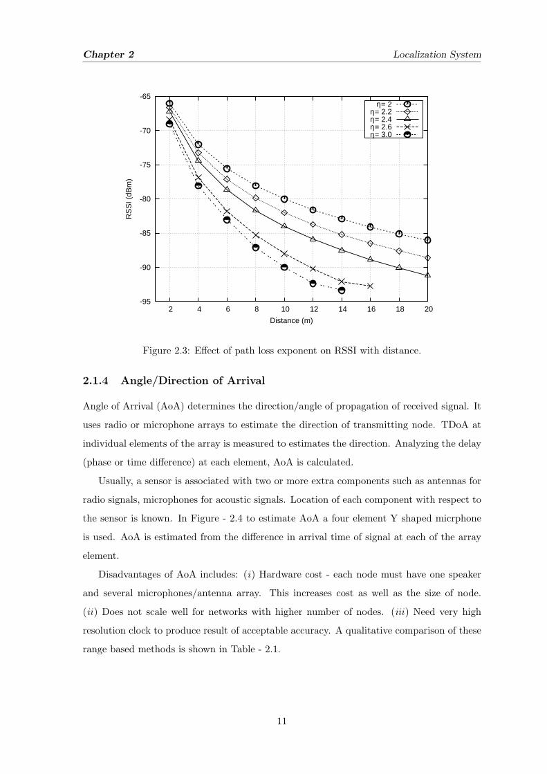
Using the above equation we can easily calculate the distance. Accuracy of RSSI depends
on the path loss model. This is because RSSI is affected by fast fading, mobility, shadows,
terrain. Savarse et al. [21] reported that the range error introduced by RSSI is ±50%.
This can be reduced by taking mean of the number of measurements at some distance.
The improper calibration of cheap radio transceiver also affects the RSSI calculation. RSSI
behaviour at different values of η is shown in Figure - 2.3.
10
Chapter 2 Localization System
-95
-90
-85
-80
-75
-70
-65
2 4 6 8 10 12 14 16 18 20
RS
SI (
dBm
)
Distance (m)
η= 2η= 2.2η= 2.4η= 2.6η= 3.0
Figure 2.3: Effect of path loss exponent on RSSI with distance.
2.1.4 Angle/Direction of Arrival
Angle of Arrival (AoA) determines the direction/angle of propagation of received signal. It
uses radio or microphone arrays to estimate the direction of transmitting node. TDoA at
individual elements of the array is measured to estimates the direction. Analyzing the delay
(phase or time difference) at each element, AoA is calculated.
Usually, a sensor is associated with two or more extra components such as antennas for
radio signals, microphones for acoustic signals. Location of each component with respect to
the sensor is known. In Figure - 2.4 to estimate AoA a four element Y shaped micrphone
is used. AoA is estimated from the difference in arrival time of signal at each of the array
element.
Disadvantages of AoA includes: (i) Hardware cost - each node must have one speaker
and several microphones/antenna array. This increases cost as well as the size of node.
(ii) Does not scale well for networks with higher number of nodes. (iii) Need very high
resolution clock to produce result of acceptable accuracy. A qualitative comparison of these
range based methods is shown in Table - 2.1.
11

Chapter 2 Localization System
α
Sensor node
Incoming signal
E1E
E
2
3
E4
Figure 2.4: Angle of Arrival.
Techniques Addational Hardware Issues Precision
AoA [22] Arrays of Microphone Directivity, Shadowing Few degrees
ToA [17] None Synchronization Centimeters (2− 5 cm)
TDoA [22] Speaker, Microphones – Centimeters (2− 5 cm)
RSSI [19] None Interference Meters (2− 3 m)
Table 2.1: A qualitative comparison of range based localization techniques.
2.1.5 Hop Count
Sensor are deployed in a fashion such that each node remains in the range of its neighbour
nodes, that is a node lies within the range R of its neighbouring node. Knowing the number
of hops (hopcount) and length of one hop (hoplength) the distance d between any two nodes
is computed as
d = (hopcount)× (hoplength) (2.8)
In the above formula, hoplength may vary, because a node may remain at any location
within the range R. Therefore, hoplength may give erroneous result. However, Kleinrock
and Silvester [23] have proposed a better estimation of hoplength if the expected number
of neighbours/node (nlocal) is known. This is given as below:
hoplength = R[1 + e−nlocal −∫ 1
−1e(nlocal/π)arccost−t
√1−t2dt] (2.9)
12

Chapter 2 Localization System
Nagpal et al. [24] have shown that the above computation works well when nlocal > 5. For
measuring distance hop count is the best metrics. However, hop count metric has some
limitation. They are: (i) Nodes not forming convex-hull may fail to find accurate hopcount.
This is because of obstacles in shortest path to neighbour as shown in Figure - 2.5, and (ii)
Distance measurement is always multiples of hoplength.
������
������
������
������
������
������
������
������
������
������
������
������
������
������
������
������
������
������
������
������
������
������
Obstacle
Figure 2.5: Distance estimation using hop count.
2.2 Position Calculation
Techniques used to estimate a node’s location are trilateration, multilateration, and trian-
gulation. Estimated distance and the position of anchor nodes is used to estimate a node’s
location.
������
������
������
������
������
������
������
������
(x
Anchor nodes
Unknown nodes
0 ,y
2(x ,y )
1(x ,y )
0)
u(x ,y ) 2
u
1
Figure 2.6: Trilateration
������
������
������
������
������������
������������
α1
2α
Figure 2.7: Triangulation
13

Chapter 2 Localization System
2.2.1 Trilateration/Multilateration
Trilateration is a geometric technique used to determine the location of an unknown node
with the help of three location aware nodes/anchor nodes. It uses distance between the
anchor nodes and the unknown node. A pictorial view of this geometric technique for
localizing an unknown node (xu, yu) with anchor nodes (xi, yi) is shown in Figure - 2.6.
Distance measurements are never perfect. As a result it is difficult to get an accurate
location. Distance measurement from more than three anchors is known as multilateration.
This technique can be used to get a unique location.
We illustrate multilateration in a 2-dimensional space with known distances between
anchor nodes and an unknown node as
d21 = (x1 − xu)2 + (y1 − yu)
2 (2.10)
d22 = (x2 − xu)2 + (y2 − yu)
2 (2.11)
...
d2n = (xn − xu)2 + (yn − yu)
2 (2.12)
Subtracting equation (2.10) from (2.11) .. (2.12) gives
d22 − d21 = x22 − x21 − 2(x2 − x1)xu + y22 − y21 − 2(y2 − y1)yu (2.13)
d23 − d21 = x23 − x21 − 2(x3 − x1)xu + y23 − y21 − 2(y3 − y1)yu (2.14)
...
d2n − d21 = x2n − x21 − 2(xn − x1)xu + y2n − y21 − 2(yn − y1)yu (2.15)
Rearranging, (2.13) .. (2.15) in matrix form, we obtain
x2 − x1 y2 − y1
x3 − x1 y3 − y1...
...
xn − x1 yn − y1
xuyu
= 12
x22 + y22 − d22 − (x21 + y21 − d21)
x23 + y23 − d23 − (x21 + y21 − d21)...
x2n + y2n − d2n − (x21 + y21 − d21)
14

Chapter 2 Localization System
Above matrix can be rewritten as
Au = b (2.16)
where
A =
x2 − x1 y2 − y1
x3 − x1 y3 − y1...
...
xn − x1 yn − y1
, u =
xuyu
, b = 12
x22 + y22 − d22 − (x21 + y21 − d21)
x23 + y23 − d23 − (x21 + y21 − d21)...
x2n + y2n − d2n − (x21 + y21 − d21)
Therefore, u can be derived as
u = (ATA)−1AT b
2.2.2 Triangulation
Triangulation is a geometric technique that uses the trigonometry laws of sine and cosines
on the angles of incoming signal α to estimate a unique location. A geometric computation
of this is shown in Figure - 2.7.
AoA measurement requires bulkier and expensive hardware such as multi-sectored an-
tennae. This makes triangulation unsuitable for small sensor nodes.
2.3 Localization algorithm
Localization algorithm is the last and most important stage of localization system. It
utilizes the information collected in previous two stages. It defines how this information can
be transformed to localize sensor nodes cooperatively. Cooperative localization refers to the
collaboration between sensor nodes to find their locations. Mostly, accuracy of this stage
is effected by the ranging method, deployment environment, and the relative geometry of
unknown nodes to the anchor nodes.
Broadly, localization algorithms in WSNs can be divided into two categories: (i) cen-
tralized, and (ii) distributed. Centralized localization requires the migration of internode
ranging and connectivity data to a sufficiently powerful central base station and then the
migration of resulting locations back to respective nodes [25]. Centralization allows an al-
gorithm to undertake much more complex mathematics than is possible in a distributed
15

Chapter 2 Localization System
setting. Whereas in distributed localization, all the relevant computations are done on the
sensor nodes themselves and the nodes communicate with each other to get their positions
in a network.
On the basis of ranging method used, localization algorithms for WSNs can be broadly
categorized into two types: (i) range based, and (ii) range free. Range based localization
algorithms use the range (distance or angle) information from the beacon node to estimate
the location [26]. Several ranging techniques exist to estimate an unknown node distance to
three or more beacon nodes. Based on the range information, location of a node is deter-
mined. Some of the range based localization algorithm includes: Received signal strength
indicator (RSSI) [19], Angle of arrival (AoA) [22], Time of arrival (ToA) [17], Time difference
of arrival (TDoA) [22].
Range-free localization algorithms use connectivity information between unknown node
and landmarks. A landmark can obtain its location information using GPS or through an
artificially deployed information. Some of the range-free localization algorithm includes:
Centroid [27], Appropriate point in triangle (APIT) [28], and DV-HOP [29]. In centroid
the number of beacon signals received from the pre-positioned beacon nodes is counted and
localization is achieved by obtaining the centroid of received beacon generators. DV-HOP
uses the location of beacon nodes, hop counts from beacons, and the average distance per
hop for localization. A relatively higher ratio of beacons to unknown nodes, and longer range
beacons are required in APIT [30]. They are also more susceptible to erroneous reading of
RSSI.
Range-based algorithms achieve higher localization accuracy, at the expense of hardware
cost and power consumption. Range-free algorithms have lower hardware cost and are more
efficient in localization. A brief review of different localization algorithms proposed in the
literature for wireless sensor networks is presented below.
Simic et al. [31] proposed a range free distributed localization algorithm, in which each
unknown node estimate its position within the intersection of bounding box of beacon nodes.
Also, they found optimal number of known nodes required to minimize the localization error
in WSN based on network area, number of nodes, and communication range (r). In their
proposed scheme a sufficient number of beacon nodes should be deployed in order to localize
entire network. Whitehouse [32] showed that the technique proposed by Simic et al. [31]
fails in the localization of non-convex network (nodes not present in convex-hull of beacons),
and under noisy range estimate.
16
Chapter 2 Localization System
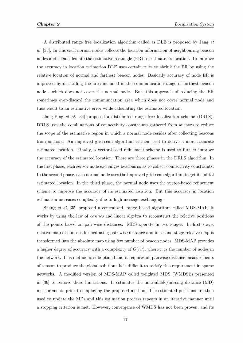
A distributed range free localization algorithm called as DLE is proposed by Jang et
al. [33]. In this each normal nodes collects the location information of neighbouring beacon
nodes and then calculate the estimative rectangle (ER) to estimate its location. To improve
the accuracy in location estimation DLE uses certain rules to shrink the ER by using the
relative location of normal and farthest beacon nodes. Basically accuracy of node ER is
improved by discarding the area included in the communication range of farthest beacon
node - which does not cover the normal node. But, this approach of reducing the ER
sometimes over-discard the communication area which does not cover normal node and
thus result to an estimative error while calculating the estimated location.
Jang-Ping et al. [34] proposed a distributed range free localization scheme (DRLS).
DRLS uses the combinations of connectivity constraints gathered from anchors to reduce
the scope of the estimative region in which a normal node resides after collecting beacons
from anchors. An improved grid-scan algorithm is then used to derive a more accurate
estimated location. Finally, a vector-based refinement scheme is used to further improve
the accuracy of the estimated location. There are three phases in the DRLS algorithm. In
the first phase, each sensor node exchanges beacons so as to collect connectivity constraints.
In the second phase, each normal node uses the improved grid-scan algorithm to get its initial
estimated location. In the third phase, the normal node uses the vector-based refinement
scheme to improve the accuracy of its estimated location. But this accuracy in location
estimation increases complexity due to high message exchanging.
Shang et al. [35] proposed a centralized, range based algorithm called MDS-MAP. It
works by using the law of cosines and linear algebra to reconstruct the relative positions
of the points based on pair-wise distances. MDS operate in two stages: In first stage,
relative map of nodes is formed using pair-wise distance and in second stage relative map is
transformed into the absolute map using few number of beacon nodes. MDS-MAP provides
a higher degree of accuracy with a complexity of O(n3), where n is the number of nodes in
the network. This method is suboptimal and it requires all pairwise distance measurements
of sensors to produce the global solution. It is difficult to satisfy this requirement in sparse
networks. A modified version of MDS-MAP called weighted MDS (WMDS)is presented
in [36] to remove these limitations. It estimates the unavailable/missing distance (MD)
measurements prior to employing the proposed method. The estimated positions are then
used to update the MDs and this estimation process repeats in an iterative manner until
a stopping criterion is met. However, convergence of WMDS has not been proven, and its
17
Chapter 2 Localization System
computational complexity is high [37].
He et al. [30] proposed a distributed, range free localization algorithm called Appropriate
Point in Triangle (APIT). In this each unknown node receive beacons from the neighbouring
anchor nodes and then construct exhaustive set of triangles using these anchor nodes. APIT
repeats Point in Triangulation (PIT) test with different combination of triangles to narrow
down the nodes estimative region. It uses a grid-scan algorithm to derive the intersection
region of all the triangles using the PIT test and then sets the center of the intersection
region as the estimated location of the normal node. APIT performs better under the high
ratio of anchors. But, as the network area is divided into large number of small square grids;
memory requirements by grid-scan algorithm to store the value of grid array is increases.
Hence make it inappropriate for memory constrained sensor nodes.
Chandrasekhar et al. [38] proposed centralized, range free area based localization scheme
(ALS). In this scheme, anchor nodes transmit signal at different power levels and each
unknown node records the lowest power level corresponding to each neighbouring anchor
node. As soon as an unknown node records power levels of four anchor nodes, it sends
the recorded vector to a sink node (powerful node). Sink then decides in which region the
reporting node lies and retransmit the same information to the reporting node.It provides
a coarse location estimate of a sensor within a certain area, rather than its exact position.
Hasebullaha et al. [39] proposed a localization algorithm using a single anchor node and
considered both the coarse grained, fine grained scenarios. In coarse grained, anchor nodes
are equipped with larger number of antennas in order to cover full network area. In fine
grained, beacon node is equipped with only one antenna, which rotates at a constant angular
velocity. In the technique proposed by Kumar and Varma [40] sensor nodes are equipped
with directional antenna in order to determine the angle (position) with respect to anchor
node.
Zhang and Yu [41] proposed a distributed, range free localization algorithm called
LSWD, in which unknown nodes are equipped with omni-directional antenna and a sin-
gle mobile beacon node is equipped with a directional antenna. The mobile beacon node
moves through the sensor area and transmit beacons (beacon node coordinates and time-
stamp when the beacon is broad-casted) to sensor nodes for localization. Based on the
collected beacon messages sensor nodes determine their locations by using the geometric
characteristics of the confined area. To localize nodes correctly LSWD uses three different
methods which include: (i) the greatest gain direction line intersection (GDDI), (ii) radiate
18

Chapter 2 Localization System
region of intersection (RROI), and (iii) the border line intersection (BLI). Although, LSWD
localizes nodes but it increases the cost of WSN as each node is equipped with an omni-
directional antennae. Its efficiency depends on the trajectory taken by the mobile beacon
node. Furthermore, with omni-directional antennae energy radiated in all directions can be
easily interfared by wide range of environment noise. This may result in high localization
error.
Khan et al. [42] proposed a distributed, iterative localization algorithm called DILOC,
in m dimensional Eucledian space Rm , that only requires only local communication. It
exploits the structure of matrix resulting from the topology of communication graph of
the network. For localization, it requires each node lies inside a convex hull of at least
(m + 1) anchor nodes. The location of each node can be computed iteratively by these
(m + 1) anchors. Basically, each node starts with a initial guess (random guess) of their
position, and then update its location estimates as a convex combination. The coefficients
o the convex combination are the barycentric co-ordinates of sensors with respect to their
neighbours, which are determined from the Cayley-Menger determinants. These are the
determinants of matrices that collect the local internode distances. Main problem with
DILOC algorithm is that normal nodes outside the convex hull of the anchor nodes are
unable to be localized.
Lee et al. [43] proposed a localization algorithm termed multiduolateration localization
(MDL) and grouping multiduolateration localization (GMDL) for indoors by employing
jumper setting of nodes. Their algorithm operate in two stages: First, edge nodes are
localized using internal division and then the remaining surface nodes, are localized using
localized edge nodes. It uses four beacon nodes placed at the corners of field. Localization
accuracy of MDL and GMDL depends on the localization of edge nodes. It results in more
error propagation as one wrongly localized edge node affects location estimation of all those
surface nodes which use it as a reference node.
Antonio et al. [44] proposed a fully decentralized, range based algorithm that allows
individual wireless nodes to iteratively refine the estimate of their position. It is based on
the combined use of convex and non-convex optimization procedures. The algorithm starts
with initialization phase where unknown node gather coordinates of adjacent anchor nodes
and corresponding distances to them. Then, it performs a convex minimization using a
gradient descent technique. This iterates until cost of the new position reaches a proper
threshold close to zero. After this a refinement step by means of vertex search heuristic is
19

Chapter 2 Localization System
accomplished. In vertex search heuristic, a minimum non-convex cost is searched among
all intersections and the selected intersection is chosen as the final node position. This
scheme ensure sensors qualifying the convex hull constraint to be globally convergent, but
the converged solution suffer from significant gap in estimation performance as compared
to optimal solution [45].
Shouhong et al. [45] proposed a distributed cooperative localization scheme and several
iterative self-positioning algorithms. They are: (i) ‘Pulled only’ - on running this algorithm
iteratively at all the sensors of the considered network, it leads to global convergence in the
sense of the global convex cost it minimizes. But, in the presence of measurement errors it
does not result in the global convergence. (ii) ‘Pulled or Pushed’ - on iteratively running this
algorithm on all the sensors of the considered network, it suffers from the local convergence.
But once correctly converged, resulted solution would be the least-square solution. (iii) A
combined version that switches between the former two algorithms iterations independently
at individual sensors based on locally collected information. It converges globally to the
least-square solution, as long as the measurement errors are sufficiently small. Efficiency of
this algorithm is heavily affected by measurement errors and it fails to localize nodes outside
the convex hull of reference nodes.
2.4 Summary
In this chapter, we discussed about the localization system. We also discussed different
components employed for localization. A brief review of different localization techniques for
static WSNs is discussed.
In the next chapter, we proposed a localization technique for static WSN, where nodes
are deployed in a grid pattern.
20

Chapter 3
Localization Using Single Anchor Node
Localization of nodes in a sensor network is essential for the following two reasons: (i) to
know the location of a node reporting the occurrence of an event, and (ii) to initiate a
prompt action whenever necessary. Different localization techniques have been proposed
in the literature. Most of these techniques use three anchor nodes for localization of an
unknown node. Increasing the number of anchor nodes will increase the overall cost of
WSN. This is because GPS enabled nodes need frequent battery replacements or a battery
of large capacity. Furthermore, GPS does not work well in indoors and dense areas/forests.
Localization techniques also differ from environment to environment. In this chapter, we
proposed a localization technique for grid environment. Sensor nodes are deployed in a grid
pattern and localization can be achieved using a single location aware or anchor node.
3.1 Proposed Technique
In this section, we proposed a distributed range based localization algorithm for a grid
environment. Since, a single anchor node is used for localization, we call this technique as
localization using single anchor node (LUSA). We made the following assumptions:
(a) Sensors are deployed in a grid pattern as shown in Figure - 3.1.
(b) We identify three types of node: (i)Beacon node: A node which can locate its own
position, and is usually equipped with GPS, (ii) Special node: Nodes which are per-
pendicular to the beacon node, and can determine their co-ordinates with respect to
beacon node. For every beacon node there exist two Special nodes, (iii) Unknown
node: Nodes which are un-aware of their location. They use localization algorithm to
determine their position. Special nodes are treated as unknown nodes.
21

Chapter 3 Localization Using Single Anchor Node
Unknown Node
Beacon Node Special Node
Figure 3.1: Deployment of Beacon node, Special node and Unknown node in a grid.
For localization, the beacon node initially broadcast its location information. Special
nodes compute their distance from the beacon node using RSSI and determine their co-
ordinates with respect to the beacon node. After computing their location information,
Special nodes also act as beacon node. Unknown nodes use trilateration mechanism to
compute their location information. We illustrate the localization process in the proposed
(a) (b)
Figure 3.2: Localization in LUSA.
scheme using Figure - 3.2. Let node 12 in the figure is a beacon node, node 13 and 17 are
special nodes, and the remaining nodes are unknown nodes. Initially, node 12 broadcast
its position. This is received by the special nodes 13 and 17 along with other unknown
nodes within the transmission range of node 12 as shown in Figure - 3.2(a). Nodes 13,
22
Chapter 3 Localization Using Single Anchor Node
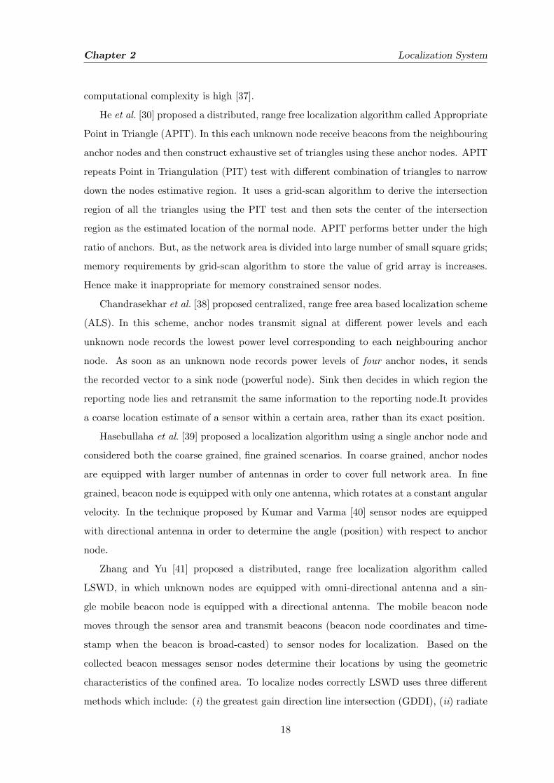
Figure 3.3: Localization pattern.
and 17 calculate their distance with respect to node 12, and localize themselves. At this
stage all the nodes within the transmission range of node 12 has the position estimate of
beacon node 12. In next stage, node 13 and 17 act as beacon nodes and broadcast their
estimated position, as shown in Figure - 3.2(b), which is received by nodes 7, 8, 11, 14, 18,
22, and 23. These nodes localize themselves using trilateration. As more and more nodes
gets localized, they act as beacon nodes. Above process continues until the whole network
is localized. Figure - 3.3 shows the progress of localization in the proposed scheme in a 9×9
grid environment. Nodes encircled with same numerical value are likely to get localized at
the same time instant.
3.2 Simulation Results
We have simulated the proposed scheme using Castalia simulator that runs on top of Om-
net++. Transmitting power of nodes is considered to be -5 dBm (0.316 mW) so as to limit
the communication range to 30 meters, and the path loss coefficient (η) to be 2.4.
A grid network of size 9 × 9 is considered for simulation. Metrics of interest are: (i)
Localization time; and (ii) Localization error - which is computed as described below:
Error =
∑N−Ri=1 ||θi − θi||
N −R
where θi is estimated position, θi is actual position, N is the total number of sensors in the
network, and R is number of beacon nodes. We have considered the following two scenarios:
23
Chapter 3 Localization Using Single Anchor Node
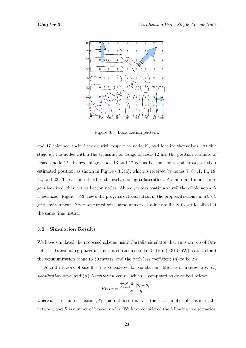
(i) Beacon node is placed at the corner of the grid as shown in Figure - 3.4, and (ii) Beacon
node is placed at the middle of the grid as shown in Figure - 3.5. In each of the above
scenarios there are one beacon node, two special nodes and many unknown nodes in the
grid.
Figure 3.4: Beacon node at the corner of
grid.
Figure 3.5: Beacon node at the middle of
grid.
Location of Beacon node Localization Time (s) Localization Error (m)
At Corner 4.636377959069 0.000175
At Middle of grid 3.422031239100 0.001892
Table 3.1: Evaluation of proposed algorithm, placing the beacon node at two different places
within the network.
Figure 3.6: Process of localization when the beacon node is placed at the middle of the grid.
The time for localization and the average localization error in the above two scenarios
24

Chapter 3 Localization Using Single Anchor Node
is shown in Table - 3.1. It is observed from the Table - 3.1, that localization error when the
beacon node is at the corner of grid is lower in comparison to placing at the center of the
grid.
0
10
20
30
40
50
60
70
80
0 10 20 30 40 50 60 70 80
0
10
20
30
40
50
60
70
80
0 10 20 30 40 50 60 70 80
(a) (b)
0
10
20
30
40
50
0 10 20 30 40 50
0
10
20
30
40
50
0 10 20 30 40 50
(c) (d)
0
10
20
30
0 10 20 30 40 50
0
10
20
30
0 10 20 30 40 50
(e) (f)
Figure 3.7: Distribution of localization error without interference in LUSA and MDL.
Localization proceeds parallely in four quadrants as shown in Figure - 3.6 when the
25

Chapter 3 Localization Using Single Anchor Node
beacon is placed at the center of the grid. As a result of parallel localization process,
localization error propagates in more than one direction resulting in increase in the average
localization error.
Next, we have compared LUSA with Multiduolateration (MDL). This is because MDL
closely resembles with LUSA. MDL is proposed for a grid environment. It works using
internal division. First, it localizes the edge nodes and then the remaining surface nodes.
In MDL, four beacon nodes are placed at the four corners of the grid. For comparison with
MDL, we also placed four beacon nodes at the four corners of the grid in LUSA. Metrices
considered for comparison are localization time and localization error. a two scenarios: (i)
without intereference, and (ii) with intereference; and the following grid sizes: (i) Square
grid of size: 9× 9, and 6× 6, and (ii) Rectangular grid of size: 6× 4, for comparison.
0.4
0.6
0.8
1
1.2
1.4
1.6
1.8
2
2.2
2.4
2.6
(6x4) (6x6) (9x5) (9x9)
Mea
n Lo
caliz
atio
n E
rror
(m
)
Grid Size
MDLLUSA
1
1.5
2
2.5
3
3.5
4
4.5
(6x4) (6x6) (9x5) (9x9)
Mea
n Lo
caliz
atio
n E
rror
(m
)
Grid Size
MDLLUSA
(a) (b)
Figure 3.8: Mean localization error (meters) in various grid: (a) Without interference, (b)
With interference.
3.2.1 Localization Error
The geographical distribution of error without interference in LUSA and MDL for different
grid size is shown in Figure - 3.7. Distribution of error in LUSA is shown in Figure - 3.7(a),
3.7(c), 3.7(e) and MDL in Figure - 3.7(b), 3.7(d), 3.7(f) for grid size of 9 × 9, 6 × 6, and
6 × 4 respectively. In each figure - dot ’•’ represents actual position of node and symbol
’×’ represents corresponding estimated position. The line joining ’•’ and ’×’ represents the
magnitude of error. From Figure - 3.7, it is observed that LUSA has lower localization error
than MDL. Higher localization error in MDL is attributed to the localization of surface
nodes. Each surface node localize itself on the basis of four nearest edge nodes (left, right,
26
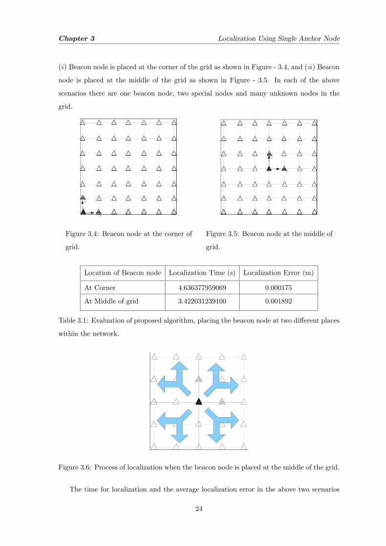
Chapter 3 Localization Using Single Anchor Node
above, below ) using internal division. Localization of each surface node is independent of
other surface nodes and depends solely on the edge nodes. Therefore, if any of the edge
node do not get its exact location, it affects the location estimation of all surface nodes
making use of that edge node for location estimation. We have shown the mean localization
error in the corresponding grids for LUSA and MDL in Figure - 3.8(a).
0
10
20
30
40
50
60
70
80
0 10 20 30 40 50 60 70 80
0
10
20
30
40
50
60
70
80
0 10 20 30 40 50 60 70 80
(a) (b)
0
10
20
30
40
50
0 10 20 30 40 50
0
10
20
30
40
50
0 10 20 30 40 50
(c) (d)
0
10
20
30
0 10 20 30 40 50
0
10
20
30
0 10 20 30 40 50
(e) (f)
Figure 3.9: Distribution of localization error with interference in LUSA and MDL.
27

Chapter 3 Localization Using Single Anchor Node
Next, we consider the effect of interference on location estimation. Effect of interference
in LUSA and MDL is shown in Figure - 3.9 where Figures - 3.9(a), 3.9(c), 3.9(e) corresponds
to LUSA and Figures - 3.9(b), 3.9(d), 3.9(f) corresponds to MDL in a grid size of 9×9, 6×6,
and 6×4 respectively. Effect of interference on the localization error in grid of different size
is shown in Figure - 3.8(b). It is observed that MDL is heavily affected in the presence of
interference as compared to LUSA.
3.2.2 Localization Time
Localization time of LUSA and MDL for different grid size is shown in Figure - 3.10. Higher
localization time in MDL is attributed to the localization of surface nodes. In MDL, local-
ization proceed in two stages : (i) First, it localizes the edge nodes, and (ii) Next, it localizes
the remaining surface nodes. In the second stage, each surface node select a reference edge
node based on shortest path. This contributes to higher localization time. Whereas, in
LUSA, localization of node’s proceeds simultaneously and does not put any constraint on
the selection of reference nodes.
0
0.5
1
1.5
2
2.5
3
3.5
(6x4) (6x6) (9x5) (9x9)
Tot
al L
ocal
izat
ion
Tim
e (s
)
Grid Size
MDLLUSA
Figure 3.10: Localization Time.
3.3 Summary
In this chapter, we proposed a localization method for grid network called LUSA. In LUSA
three types of nodes are identified. They are anchor, special and unknown nodes. For every
anchor there are two special nodes and they are placed perpendicular to the anchor node.
Localization in LUSA is achieved using a single beacon node and two special nodes. LUSA
28

Chapter 3 Localization Using Single Anchor Node
is compared with MDL, which is also a localization technique proposed for grid network.
It is observed that the proposed scheme has lower localization error and lower localization
time in comparison with MDL.
29

Chapter 4
Distributed Binary Estimation Approach
4.1 Introduction
Most of the existing localization techniques use three or more anchor nodes for localizing
a single unknown node except for those schemes where directional antenna is used. In the
scheme using directional antenna [39] algorithmic complexity, size and cost of node is more.
In this chapter, we propose a range based localization algorithm for sensor networks in a grid
environment. The proposed technique localizes an unknown node using two anchor/location-
aware nodes.
4.2 Distributed Binary Node Localization
In this section, we proposed a node localization technique called Distributed Binary Node
Localization Estimation (DBNLE). The proposed localization technique is distributed in
nature. We call it binary, because each unknown node other than the edge nodes (placed
with respect to anchor node) use two location aware nodes in the localization process. The
following assumptions are made in DBNLE:
(i) Nodes are deployed in a grid.
(ii) Distance between the grid points are set as per the RSSI requirement.
(iii) Nodes are classified into three types: (a) Anchor node: Nodes whose position is known
either through GPS or manually built-in. In DBNLE there is one anchor node. (b) Un-
known node: Node which use localization technique to determine its position. (c) Set-
tled node: These are the nodes that have obtained their location information through
a localization technique. They serve as an anchor node for the remaining unknown
nodes. Deployment of nodes in a grid is shown in Figure 4.1.
30

Chapter 4 Distributed Binary Estimation Approach
0 21
15
3
13 14
Anchor Node Unknown Node
7 8 9
1210 11
4
5
6
Figure 4.1: Deployment of nodes in a grid, showing the placement of anchor and unknown
nodes.
DBNLE operate in three phases: (i) First phase: Edge nodes with respect to anchor
node get localized and become settled nodes, (ii) Second phase: Settled nodes broadcast
their position, and (iii) Third phase: Unknown node gets localized after obtaining position
and range measurements from any two settled nodes. Phase Two and Three continues until
all nodes get localized. Localization of edge nodes is explained in Subsection 4.2.1 and the
remaining unknown nodes in Subsection 4.2.2.
4.2.1 Localization of Edge nodes
Lines 13− 16 in Algorithm 1 explain localization of edge nodes. We consider Figure 4.1 to
illustrate localization of edge nodes. In Figure 4.1, node 0 is the anchor node, and nodes
1, 2, 3, 4, 5, and 6 are the edge nodes. Let (x0, y0) be the location of anchor node 0. On
receiving location information from the node 0, node 1, and node 4 gets localized. Node 1
compute its co-ordinate as follows:
x1 = x0 + distance between node 0 and 1,
y1 = y0.
Node 4 compute its position as:
x4 = x0,
y4 = y0 + distance between node 0 and 4.
31

Chapter 4 Distributed Binary Estimation Approach
Algorithm 1: DBNLE Localization algorithmInput: Nen: Edge node with respect to Anchor node, Nr: Nodes other than Nen, A: Anchor node
1 beaconSet← ϕ /* Set of received locations */
2 rBeacon← 0 /* Number of received beacons */
3 flag ← 0 /* Set to 1, if node gets localized */
4 dist[2]← −1 /* Array for storing distances */
5 Initialization:
6 if n ∈ A then /* If this is an anchor node */
7 Broadcast beacon
8 Input:
9 msg ← beacon
10 dist← distanceEstimation(msg)
11 increment rBeacon
12 Action:
13 if n ∈ Nen then
14 estimate Position using msg and dist
15 broadcast beacon
16 flag ← 1
17 else if (n ∈ Nr) and (rBeacon < 2) then
18 beaconSet← beaconSet ∪msg
19 dist[rBeacon]← dist
20 if dist[rBeacon] = dist[−−rBeacon] then /* Check distance constraint */
21 delete dist[rBeacon]
22 delete recent msg from beaconSet
23 decrement rBeacon
24 if rBeacon = 2 then
25 estimate Position using dist[2] and beaconSet
26 broadcast beacon
27 flag ← 1
Description of Algorithm 1: Localization in DBNLE starts with a beacon broadcast
by an anchor node as shown in lines 6 – 7. Lines 13 – 16 represent localization of edge
nodes and simultaneously acting as settled nodes. Lines 17 – 27 represent localization of
unknown nodes as soon as they receive beacons from two non-equidistant settled nodes.
32
Chapter 4 Distributed Binary Estimation Approach
After computing their location information, node 1 and 4 become settled node. Node 2
and 3 gets localized as node 1 on receiving location information from node 1 and node 2
respectively. Node 5 and 6 gets localized as in node 4 on receiving location information from
node 4 and 5 respectively.
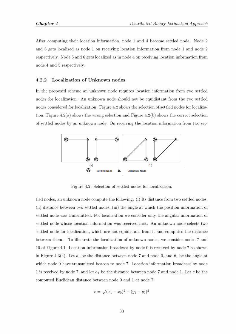
4.2.2 Localization of Unknown nodes
In the proposed scheme an unknown node requires location information from two settled
nodes for localization. An unknown node should not be equidistant from the two settled
nodes considered for localization. Figure 4.2 shows the selection of settled nodes for localiza-
tion. Figure 4.2(a) shows the wrong selection and Figure 4.2(b) shows the correct selection
of settled nodes by an unknown node. On receiving the location information from two set-
Figure 4.2: Selection of settled nodes for localization.
tled nodes, an unknown node compute the following: (i) Its distance from two settled nodes,
(ii) distance between two settled nodes, (iii) the angle at which the position information of
settled node was transmitted. For localization we consider only the angular information of
settled node whose location information was received first. An unknown node selects two
settled node for localization, which are not equidistant from it and computes the distance
between them. To illustrate the localization of unknown nodes, we consider nodes 7 and
10 of Figure 4.1. Location information broadcast by node 0 is received by node 7 as shown
in Figure 4.3(a). Let b1 be the distance between node 7 and node 0, and θ1 be the angle at
which node 0 have transmitted beacon to node 7. Location information broadcast by node
1 is received by node 7, and let a1 be the distance between node 7 and node 1. Let c be the
computed Euclidean distance between node 0 and 1 at node 7.
c =√
(x1 − x0)2 + (y1 − y0)2
33

Chapter 4 Distributed Binary Estimation Approach
1
0 1
7
θ14
5 10a2
θ2
c b2a
1b
c
(b)(a)
Figure 4.3: Localization of unknown nodes 7 and 10
0 1
15
3
13 14
2
1 2
8 973
4
0
2
45
78
89
56
11125
0
4
1110
5 10 11 12
6
Anchor Node Unknown Node
Settled Sources
201
1
Figure 4.4: Nodes involved in the localization of unknown nodes in a 4 x 4 grid.
where (x0, y0) is the location of node 0, and (x1, y1) is the location of node 1. Similarly,
unknown node 10 receives location information from nodes 4 and 5 as shown in Figure
4.3(b). Let θ2 be the angle at which node 4 have transmitted beacon to node 10. The angle
θ1 and θ2 is computed as follows:
θ1 = cos−1((b12 + c2 − a1
2)/2b1c).
θ2 = 90◦ − (cos−1((b22 + c2 − a2
2)/2b2c)).
Let (x7, y7) and (x10, y10) be the co-ordinates of nodes 7 and 10 respectively. Node 7
compute its co-ordinate (x7, y7) as follows:
34

Chapter 4 Distributed Binary Estimation Approach
0 1
15
3
13 14
2
8 974
5 10 11 12
6
Anchor Node
1 3 6
2 4 7 10
5 8 12 13
9 11 14 15
Unknown Node
Localizing Order
Figure 4.5: Localization pattern in a 4 x 4 grid.
��������
���������
���������
0 1 2 3 4 5
6 7 8 9 10 11
12 13 14 15 16 17
19 20 22 23
A(0,0) AB(x ,0)
E(xA, yA)A)C(0,y
P(x,0)
21)
18
General NodeAnchor Node Edge Node
AQ(x’,y
��������
������
������
���������
���������
������������
������
������
��������
������
������
0 1 2 3 4 5
6 7 8 9 10 11
12 13 14 15 16 17
19 20 22 23
A(0,0) AB(x ,0)
E(xA, yA)A)C(0,y
P(x,0)
21)
18AQ(x’,y
Wrong Estimated PostionCorrect Estmated Position
(a) (b)
Figure 4.6: Localization process in MDL: (a) Localization of edge nodes, (b) Localization
of surface nodes using nearest edge nodes.
x7 = x0 + b1 ∗ cosθ1
y7 = y0 + b1 ∗ sinθ1
Similarly, node 10 compute its co-ordinates (x10, y10) as follows:
x10 = x4 + b2 ∗ cosθ2
y10 = y4 + b2 ∗ sinθ2
The above process continues until all nodes are localized. Figure 4.4 shows the progress of
localization in a 4 × 4 grid. Rectangular box to the right of each node shows the settled
nodes used for its localization. Figure 4.5 shows the localization pattern i.e., the order in
35

Chapter 4 Distributed Binary Estimation Approach
which unknown nodes are localized in a 4 x 4 grid. Rectangular box to the right of each
node shows its corresponding localization order.
4.3 Simulation Results
We have simulated DBNLE, using Castalia simulator [46] that runs on the top of the Om-
net++ and compared with a closely related scheme called Multiduolateration (MDL) [43].
Metrics considered for comparison are: (i) Accuracy in location estimation, and (ii) Time
required for localization. Localization of MDL is shown in Figure 4.6. It works in two
phases: (i) First phase: In this phase edge nodes are localized using internal division as
010
2030
4050 0
510
1520
2530
0
0.2
0.4
0.6
0.8
1
Err
or
(m)
X Coordinate (m)
Y Coordinate (m)
Err
or
(m)
0
0.02
0.04
0.06
0.08
0.1
0.12
0.14
0.16
0.18
010
2030
4050 0
510
1520
2530
0
0.2
0.4
0.6
0.8
1E
rror
(m)
X Coordinate (m)
Y Coordinate (m)
Err
or
(m)
0
0.02
0.04
0.06
0.08
0.1
0.12
0.14
(a) (b)
010
2030
4050 0
10
20
30
40
50
0
0.2
0.4
0.6
0.8
1
1.2
Err
or
(m)
X Coordinate (m)
Y Coordinate (m)
Err
or
(m)
0
0.2
0.4
0.6
0.8
1
1.2
010
2030
4050 0
10
20
30
40
50
0
0.2
0.4
0.6
0.8
1
1.2
Error(m)
X Coordinate (m)
Y Coordinate (m)
Error(m)
0
0.2
0.4
0.6
0.8
1
1.2
(c) (d)
0 10 20 30 40 50 60 70 80 010
2030
4050
6070
80
0
2
4
6
8
10
Err
or
(m)
X Coordinate (m)
Y Coordinate (m)
Err
or
(m)
0
1
2
3
4
5
6
7
8
9
0 10 20 30 40 50 60 70 80 010
2030
4050
6070
80
0
2
4
6
8
10
Err
or
(m)
X Coordinate (m)
Y Coordinate (m)
Err
or
(m)
0
0.2
0.4
0.6
0.8
1
1.2
1.4
1.6
(e) (f)
Figure 4.7: Geographical distribution of error for a grid size of 6 × 4, 6 × 6, and 9 × 9 is
shown in a, c, and e respectively for MDL and b, d, and f respectively for DBNLE.
36

Chapter 4 Distributed Binary Estimation Approach
shown in Figure 4.6(a), and (ii) Second phase: In this phase surface nodes are localized
using four nearest edge nodes (left edge node, right edge node, above edge node, below edge
node) as shown in Figure 4.6(b). Parameters considered for simulation are given below:
(i) Path loss coefficient (η) = 2.4.
(ii) Distance between successive nodes = 10 meters.
(iii) Number of anchors nodes = 4. They are placed at the corners of the grid.
RSSI technique is used for ranging. Grid of size 6 × 4, 6 × 6, 9 × 9 is considered for
comparison.
4.3.1 Localization Error
The geographical distribution of error in MDL and DBNLE for grid of different size is shown
in Figure 4.7. Distribution of error in MDL for grid size of 6 × 4, 6 × 6, 9 × 9 is shown in
Figure 4.7(a), 4.7(c), 4.7(e) respectively, Distribution of error in DBNLE for the grid size of
6 × 4, 6 × 6, 9 × 9 is shown in Figure 4.7(b), 4.7(d), 4.7(f) respectively. Figure 4.7 depicts
the distribution of location error, where the peaks indicate magnitude of error in estimated
position vis-a-vis their real position. It is observed from the Figure that the magnitude of
peaks are lower in DBNLE compared to that of MDL. This is because in MDL each surface
node required location information from four edge nodes for localization. Any error in the
localization of edge node, propagates to the surface nodes to a greater extent.
Figure 4.6 illustrate the error propagation in MDL. Suppose there is an error in the
localization of edge nodes 2 and 21 as shown in Figure 4.6(a). Localization of node 15
requires the location information of edge nodes 3, 12, 17, and 21. Since there is an error in
the localization of 21, this error contributes to the localization error of node 15. Similarly,
node 9 will be wrongly localized. Localization error in node 2, leads to localization error
in node 8 and 14. In DBNLE, an unknown node needs only two node for localization as
compared to four nodes in MDL. As a result the cumulative error propagation is lesser in
DBNLE.
4.3.2 Localization Time
Localization time refers to the time required for the localization of the whole network.
Localization time of both MDL and DBNLE for different grid size is shown in Figure 4.8.
37

Chapter 4 Distributed Binary Estimation Approach
0
0.5
1
1.5
2
2.5
3
3.5
(6x4) (6x6) (9x9)
Loca
lizat
ion
Tim
e (s
)
Grid Size
MDLDBNLE
Figure 4.8: Localization time of MDL vs. DBNLE in different grid sizes.
It is observed that MDL takes more time for localization than DBNLE. This increase in
localization time is attributed to the shortest path algorithm used by each surface node for
the selection of its reference edge nodes.
4.4 Summary
In this chapter we proposed a localization method called distributed binary node localization
estimation (DBNLE) for grid network. Three types of node are identified in DBNLE. They
are: anchor node, settled node, and unknown node. For localization, an unknown node
require two settled nodes. An unknown node becomes settled node after obtaining location
information. Localization can be achieved using a single anchor node. DBNLE is compared
with a similar scheme called multi-duolateration (MDL) also proposed for grid. It is observed
that the DBNLE has lower localization error and localization time compared to MDL.
In the next chapter we proposed a localization technique for mobile WSN.
38

Chapter 5
Dead Reckoning Technique
5.1 Introduction
Mobility of sensor nodes increase the applicability of wireless wensor networks (WSNs).
Mobility of sensor nodes with respect to environment can be of two types: (i) static, and
(ii) dynamic. In both the case, sensor node is either fixed to a carrier like zebras in a
zebranet [2], or placed on a robotic platform. In static case, a sensor node is only data
driven, i.e., to sense the environment and report to the base station (BS). In dynamic case,
a sensor node is not only data driven, but also serve as an actuator. Whether it is static
or dynamic, the position of nodes changes oftenly. As a result a node in mobile WSNs is
localized more than once, compared to static WSNs - where a node is localized only once at
the initialization of network. The continuous localization of nodes with mobility results in:
(i) faster battery deletion and hence reduces the lifetime of sensor nodes, (ii) increase in the
communication cost. On the contrary, mobility improves: (i) coverage of WSN - uncovered
locations at one instant can be covered at some other instant of time, (ii) enhances the
security - intruders can be detected easily as compared to the static WSNs, (iii) increases
connectivity - mobility increases the neighbours of a node [13].
A mobile WSN can be in one of the following scenarios [15,47–58]:
1. Normal nodes are static, and seeds are moving : In this scenario, mobile anchor nodes
(≥ 1) continuously broadcast their location. As soon as a static node receives three or
more than three beacons, it localizes itself. Accuracy and localization time depends
mostly on the trajectory followed by the seeds.
2. Normal nodes are moving, and seeds are static: In this scenario, each normal node is
expected to receive the beacons at the same instant of time. Otherwise, it will result in
inaccurate estimated location. With time span the previous estimated location become
39
Chapter 5 Dead Reckoning Technique
obsolete. As a result nodes localize repeatedly at fixed intervals with new received
seed locations. One of the best example for this scenario is a battlefield, where normal
nodes are attached to military personnel and seeds are fixed as landmarks within the
battlefield. This not only helps in detecting the current position but also helps in
providing feedback from a particular area of battlefield.
3. Both the normal nodes and seeds are moving : This scenario is the most versatile and
complex among all the three. In this, the topology of the network changes very often.
It is difficult for a normal node to get fine grained location. Therefore, the localization
error is comparatively higher than the previous two scenarios.
In this chapter, we present a localization algorithm for third scenario, i.e., for a network
where all the nodes are mobile. We consider this scenario because: (i) a little emphasis has
been given, owing to its complexity, (ii) to the best of our knowledge whatever little local-
ization techniques has been proposed for this scenario have used the range free techniques
only for estimating the distance between nodes. In the propose technique we have used a
range based technique for distance estimation between the mobile nodes.
5.2 Related work
Although a rich literature is available for localization in static WSN, not enough attention
has been drawn for the localization of mobile WSN, owing to the complexity added due to
the node mobility. Most of the existing localization techniques for mobile WSN use Monte-
Carlo localization (MCL) approach, which is not only time-consuming but also memory
intensive. A brief review of different localization algorithms proposed in the literature for
mobile sensor networks is presented below.
Tilak et al. [59] proposed two classes of localization approach: (i) Adaptive, and (ii)
Predictive; for mobile WSNs considering the accuracy as well as energy requirement. Adap-
tive localization dynamically adjusts the localization period based on the recent observed
motion of the sensor, obtained from examining the previous locations. This approach al-
lows a sensor to reduce its localization frequency when it is slow, or increase when it is fast.
In the predictive approach, a sensor estimate the motion pattern and project its motion
in future. If the prediction is accurate, which occurs when nodes are moving predictably,
location estimation may be generated without performing actual localization. This reduces
the localization frequency thereby saving energy.
40

Chapter 5 Dead Reckoning Technique
Bergamo and Mazzimi [51] proposed a range based algorithm for localizing mobile WSNs.
They used fixed beacons which are placed in two corners on the same side of a rectangular
space, whose signals are used by mobile sensors to compute their relative position. Sensors
estimate their power level from the received beacon and estimate their position by triangu-
lation method. They also studied the effect of mobility and fading in finding the accurate
position.
Hu and Evans [15] proposed a range free technique based on Monte-Carlo localization
(MCL). This technique is used for the localization of robots in a predefined map. It work
in two steps: First, it represent the possible locations of an unknown node with a set of
weighted samples and in the next stage, invalid samples are filtered out by incorporating
the newly observed samples of seed nodes. Once enough samples are obtained, an unknown
node estimate its position by taking the weighted average of the samples. In this technique,
the sample generation is computationally intensive and iterative process. This also needs a
higher density of seeds.
Aline et al. [60] proposed a scheme to reduce the sample space generated in [15]. They
named it as Monte-Carlo Boxed (MCB) scheme. The sample generation is restricted within
the bounding box, which is built using 1-hop and 2-hop neighbouring anchor nodes. The
neighbouring anchor information is also used in the filtering phase. Therefore, it reduces the
number of iterations to construct the sample set. However, the localization error in MCB
is not reduced if the number of valid samples is same as that in MCL.
Rudafshani and Datta [61] proposed two algorithms called MSL and MSL* which are
based on MCL technique. MSL* localizes mobile as well as static sensor nodes. It uses
sample set of all 1-hop and 2-hop neighbours of normal nodes and anchor nodes. This
resulted in better estimation of position with increased memory requirements and increased
communication cost. In MSL, a node weight its samples using the estimated position of
common neighbour nodes. MSL* outperforms MSL in most scenarios, but incurs a higher
communication cost. MSL outperforms MSL* when there is significant irregularity in the
radio range. Accuracy of common neighbour nodes is determined by their closeness value.
Closeness value for a node P with N samples is computed as:
ClosenessP =
∑Ni=1Wi
√(xi − x)2 + (yi − y)2
N
where (x, y) is P’s estimated position and (xi, yi) is P’s ith sample with weight Wi. Both
MSL and MSL* need higher anchor density and node density. Also, when vmax (maximum
41

Chapter 5 Dead Reckoning Technique
velocity) is large, performance of both MSL and MSL* reduces to a greater extent. Further-
more, the size of bounding box for the generation of samples is reduced in [62], using the
negative constraint of 2-hop neighbouring anchor nodes. This reduces the computational
cost of obtaining samples, and a higher location accuracy is achieved under higher density
of common nodes.
Wang et al. [63] proposed RSS based MCL scheme to sequentially estimate location of
mobile nodes. First, it uses a set of samples with related weights to represent the posterior
distribution of node’s location. Next, it estimates the node’s location recursively from
the RSS measurements within a discrete state-space localization system. Accuracy of this
scheme depends on the number of samples used and the log normal statistical model of RSS
measurements. Comparison of these techniques is shown in Table 5.1.
PROPOSALS Nature Technique Used Mobility Model Comments
Tilak et al. [59] Range Free Triangulation Random Waypoint Model, Gaus-
sian Markovian Model
Foccused more on localization
frequency.
Bergamo et al. [51] Range
Based
Triangulation Random Waypoint Model (RWP) Puts a limit on the localization
area.
Evans et al. [15] Range Free Sequential MCL Random Waypoint Model, Refer-
ence Point Group Model [64]
MCL does not converge fastly
in slow WSN’s.
Aline et al. [60] Range Free MCL Boxed Modified RWP with pause time =
0 & minimum node speed = 0.1
m/s
Does not improve if no. of sam-
ples same as in MCL.
Datta et al. [61] Range Free Particle filtering ap-
proach of MCL
Modified RWP with pause time =
0 seconds
Computationally intensive &
high communication cost.
Wang et al. [63] Range
Based
Sequential MCL Random Waypoint Model Accuracy depends on the qual-
ity of samples used and RSSI
model.
Table 5.1: Comparison of different localization techniques for Mobile WSN’s
5.3 Proposed Localization Technique
In this section, we propose a range based, distributed localization algorithm for mobile
WSNs. The proposed technique is called Dead Reckoning Localization Technique (DRLMSN).
In DRLMSN nodes are classified into the following three types: (i) Anchor node (A): A node
which can locate its own position, and is usually equipped with GPS, (ii) Normal/unknown
node (U): Nodes which are unaware of their location, and uses localization algorithm to
determine their position, (iii) Settled node (S): These are the normal nodes that have ob-
tained their location information through a localization technique. They serve as an anchor
node for the remaining unknown nodes.
To localize normal mobile nodes accurately with the help of mobile anchor nodes is a
42

Chapter 5 Dead Reckoning Technique
difficult task. This is because the transmitter as well as the receiver changes their position
at every time instant. Therefore, to localize, a normal node must receive the beacons from
all the neighbouring nodes at the same time instant. A beacon is the frequent advertisement
from anchor/settled nodes. This advertisement contains the anchor/settled node identify,
and location. Continuous localization of mobile nodes drains their battery power at a faster
rate which ultimately reduces the lifetime of sensor nodes.
In DRLMSN, sensor nodes are localized during a time interval called checkpoint. There
are two localization phases in DRLMSN. First phase is called Initialization phase. In this
phase, a node is localized using trilateration mechanism. A node remains in the initialization
phase until it localizes using trilateration mechanism. The subsequent localization phase
is called Sequent phase. In this phase a node localizes itself using only two anchor nodes.
Bezout’s theorem is used to estimate locations of a node. A dead reckoning approach is
used to identify their correct estimated position. Once a node is localized in either of the
above two phases, it act as settled node and broadcasts a beacon during the checkpoint.
Initialization and Sequent phases are explained below.
5.3.1 Initialization Phase:
During the checkpoint, each anchor node broadcasts a beacon. A normal node localizes itself
for the first time during the checkpoint by using three anchor nodes. As soon as, a node
localizes, it broadcasts a beacon during the same checkpoint. This results in the localization
of one/two beacon deficit nodes. This process continues until the end of the checkpoint.
At the end of the checkpoint, some nodes fail to localize. The possible reasons for
localization failure and the corresponding actions to be taken are: i) A normal node receives
only one (or two) beacon. In this case, normal node deletes the received beacons and moves
on. In the next checkpoint it attempt to localize using three beacons. ii) A normal node
receives no beacon. In this case, a node moves on and tries to localize itself in the next
checkpoint using three beacons.
5.3.2 Sequent Phase:
A node goes to the sequent phase after localization using trilateration mechanism. In this
phase, each normal node localizes with only two nearest location aware nodes (anchor /
settled node). As the normal node receives two beacons, it estimates two positions using
43

Chapter 5 Dead Reckoning Technique
Bezout’s theorem. According to Bezout’s theorem “The intersection of a variety of degree
m with a variety of degree n in complex projective space is either a common component or it
has mn points when the intersection points are counted with the appropriate multiplicity.”
Position estimation of a node using Bezout’s theorem is explained below.
Let (x, y) be the position of an unknown node and (a1, b1), (a2, b2) be the position of
two of its neighbouring anchor nodes. Also, let the distance between an unknown node and
the respective anchor nodes be d1 and d2 respectively. Then,
(x− a1)2 + (y − b1)
2 = d12 (5.1)
(x− a2)2 + (y − b2)
2 = d22 (5.2)
On re-arranging (5.1) and (5.2),
x2 + y2 = d12 − a1
2 − b12 + 2a1x+ 2b1y (5.3)
x2 + y2 = d22 − a2
2 − b22 + 2a2x+ 2b2y (5.4)
On comparing, (5.3) and (5.4), we have
d12 − a1
2 − b12 + 2a1x+ 2b1y = d2
2 − a22 − b2
2 + 2a2x+ 2b2y (5.5)
2(a1 − a2)x = (d22 − a2
2 − b22 − d1
2 + a12 + b1
2) + 2(b2 − b1)y (5.6)
Let z0 = d22 − a2
2 − b22 − d1
2 + a12 + b1
2
The eqation (5.6) can be reduced to
x =z0 + 2(b2 − b1)y
2(a1 − a2)(5.7)
For simplification, this can be written as
x = z + py (5.8)
where z =z0
2(a1 − a2), and p =
2(b2 − b1)
2(a1 − a2)On substituting the value of x in equation (5.1), we obtained
(p2 + 1)y2 + (2zp− 2a1p− 2b1)y − (d12 − a1
2 − b12 − z2 + 2a1z) = 0 (5.9)
Solving the quadratic equation (5.9), we obtain y1 and y2. Let x1 and x2 be the values
corresponding to y1 and y2 respectively. Therefore, the proposed algorithm estimates two
positions P1 (x1, y1) and P2 (x2, y2).
44

Chapter 5 Dead Reckoning Technique
In order to select the correct estimated position a dead reckoning approach is used.
In this approach, a localized node say k uses its location pprev at the checkpoint ti to
estimate its location in the next checkpoint at ti+1 . Let v be the velocity and t be the
time duration between the two successive checkpoints. Then, the distance d traveled by
the node k between two successive checkpoints is calculated as d = v ∗ t . Therefore, at the
checkpoint ti+1 , an unknown node knows its position at checkpoint ti and the distance d
traveled between the two successive checkpoints. Also, the node has two anchor positions,
i.e., (a1, b1), (a2, b2). Node uses trilateration to calculate the position P(x, y). Then the
node computes the correction factor Cf to select one of the two estimated positions P1 and
P2 . The correctness factor is computed as:
Cf1 =√
(x− x1)2 + (y − y1)2
Cf2 =√
(x− x2)2 + (y − y2)2
where Cf1, Cf2 represents the distance of position P1 , and P2 from the position P estimated
via trilateration. The correct position of the node is P1 (x1, y1) if Cf1 < Cf2 else the correct
position is P2 (x2, y2). This is because, calculated position P(x, y) always deviates from the
actual position by a small margin. Once a node is localized, it broadcasts a beacon. This
process continues until the end of the checkpoint.
(a) (b)
6
1
2
0
4
8
76
5
3
54
5
6
3
4
2
1
7
1 2 3 4 5 6 7 8
1
2
3
4
5
7
8
9
10
0 9 10
1
2
3
4
5
6
7
8
9
10
0 1 2 3 6 7 8 9 10
Anchor node Settled nodeNormal node
08
Figure 5.1: Initialization phase: (a) At the first checkpoint, anchor nodes transmit beacons
and normal nodes localize via trilateration; (b) normal nodes that are short of 1 or 2 beacons
localize with the help of settled nodes.
45

Chapter 5 Dead Reckoning Technique
54
5
6
3
4
2
1
7
1
2
3
4
5
6
7
8
9
10
0 1 2 6 7 8 9 10
08
141 2 3 4 5 6 7 8 9 10 11 12 13
6
Estimated positions
P2
P
2
Cf1
14
16
0
7
8
5
2P
Cf
Position estimated by trilateration
3
At checkpoint (t i+1)
0
)At checkpoint (t i
d
1
2
3
4
5
8
10
9
7
(a) (b)
Figure 5.2: Normal node 3 at checkpoint ti+1 estimate two locations P1 and P2 using two
anchor nodes 0 and 2. The correct position is selected by using the previous position of
node 3 at checkpoint ti .
We illustrate the localization in proposed scheme using Figure 5.1. Localization in the
initialization phase is shown in Figure 5.1(a) and 5.1(b). Node 3 in Figure 5.1(a) receives
beacon from three anchor nodes 0, 1, and 2 at checkpoint ti and localizes. Nodes 4 and
7 receives only two beacon, whereas nodes 5, 6, and 8 receives only one beacon. These
nodes at this point of checkpoint ti can not localize, as the number of beacons required for
localization for the first time is three. Node 3 broadcast a beacon after localization. Nodes 4
and 7 gets localized after receiving beacon from node 3. This is shown in Figure 5.1(b). This
co-operative, distributive process of localization continues until the end of the checkpoint.
At the end of the checkpoint ti, nodes 6 and 8 have only one beacon. Both these nodes
delete the beacons and continue moving.
Figure 5.2(b) illustrate the sequent phase at checkpoint ti+1. We consider node 3, to
explain localization using two anchor nodes. Let the co-ordinate of node 3 at checkpoint
ti be (5.5, 6.3) as shown in Figure 5.2(a), and the distance traveled during the checkpoint
interval ti and ti+1 be 3.5 unit. At checkpoint ti+1, node 3 can be localized using two anchor
nodes 0 and 2, this is shown in Figure 5.2(b). Let the co-ordinate of node 0 and 2 be (7, 8)
and (11, 6) respectively as shown in Figure 5.2(b). Using Bezout’s theorem node 3 estimate
two locations P1 (8.54, 5.54) and P2 (9.98, 8.24). To select one of the above two locations
dead reckoning approach is used. Based on the location of node 0, node 2 and its previous
location, node 3 estimates its new location P(x, y) equal to (8.78, 6.03) using trilateration
46
Chapter 5 Dead Reckoning Technique
technique. Then node 3 calculates the correctness factor Cf1 and Cf2 to find the least
deviated estimated position from P(x, y). The computed value of Cf1 and Cf2 is 0.738 and
2.514 respectively. Since Cf1 < Cf2 the position P1 (8.54, 5.54) is selected as the correct
estimated position. It can be observed from the Figure 5.2(b) the actual position of node 3
is very close to the estimated position.
The proposed localization algorithm is given as Algorithm 1.
47
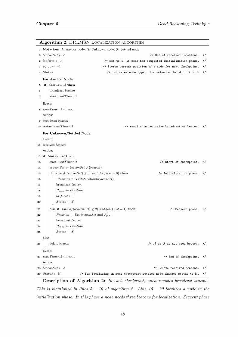
Chapter 5 Dead Reckoning Technique
Algorithm 2: DRLMSN Localization algorithm
1 Notation: A: Anchor node, U : Unknown node, S: Settled node
21 beaconSet← ϕ /* Set of received locations. */
2 locfirst← 0 /* Set to 1, if node has completed initialization phase. */
3 Pprev ← −1 /* Stores current position of a node for next checkpoint. */
4 Status /* Indicates node type: Its value can be A or U or S */
For Anchor Node:
5 if Status = A then
6 broadcast beacon
7 start waitT imer 1
Event:
8 waitT imer 1 timeout
Action:
9 broadcast beacon
10 restart waitT imer 1 /* results in recursive broadcast of beacon. */
For Unknown/Settled Node:
Event:
11 received beacon
Action:
12 if Status = U then
13 start waitT imer 2 /* Start of checkpoint. */
14 beaconSet← beaconSet ∪ {beacon}
15 if (sizeof(beaconSet) ≥ 3) and (locfirst = 0) then /* Initialization phase. */
16 Position← Trilateration(beaconSet)
17 broadcast beacon
18 Pprev ← Position
19 locfirst← 1
20 Status← S
21 else if (sizeof(beaconSet) ≥ 2) and (locfirst = 1) then /* Sequent phase. */
22 Position← Use beaconSet and Pprev
23 broadcast beacon
24 Pprev ← Position
25 Status← S
else
26 delete beacon /* A or S do not need beacon. */
Event:
27 waitT imer 2 timeout /* End of checkpoint. */
Action:
28 beaconSet← ϕ /* Delete received beacons. */
29 Status← U /* For localizing in next checkpoint settled node changes status to U. */
Description of Algorithm 2: In each checkpoint, anchor nodes broadcast beacons.
This is mentioned in lines 5 – 10 of algorithm 2. Line 15 – 20 localizes a node in the
initialization phase. In this phase a node needs three beacons for localization. Sequent phase
48

Chapter 5 Dead Reckoning Technique
localization is mentioned in lines 21 – 25. In this phase a node require only two beacon
node for localization. Timer 1 causes anchor nodes to broadcast beacon at the start of each
checkpoint recursively. Timer 2 controls duration of each checkpoint.
5.4 Performance Evaluation
We have simulated the proposed scheme using Castalia simulator [46] that runs on the
top of OMNET++. We made the following assumptions in our simulation: (i) nodes are
considered to be homogeneous, with respect to transceiver power and receiver sensitivity.
This helps in controlling the connectivity between nodes in the network easily; (ii) for
simplicity, we consider transmission range of all the nodes as a perfect circle. This ensures
that beacon packets transmitted by a neighbouring node are always received successfully;
(iii) all sensor nodes are synchronized.
The key metric used for evaluating the localization algorithm is the accuracy in location
estimation. We calculated the estimated error as the difference between the estimated
position and the actual position. The average root mean square error (RMSE) is calculated
as:
Average RMSE =
∑N−Pi=1 ||θi − θi||
N − P
where θi is estimated position, θi is actual position, N is the total number of nodes in the
network, and P is number of anchor nodes.
We consider the following parameters in our simulation: (i) nodes are randomly deployed
in a sensor field of area 200×200 m2; (ii) symmetric communication and the communication
range is 20 meters; (iii) anchor node density is 10%. We define the anchor density as the
ratio between the anchor nodes to the total nodes in the network; (iv) transmission power is
-5 dBm; (v) path loss exponent (η) is 2.4; (vi) modified random waypoint mobility model [65]
and random direction mobility model [66] are used. We compared DBNLE with another
range based scheme called as RSS-MLE [63]. Through simulation, we studied the impact
of mobility model, anchor density, node speed, number of normal nodes, and deployment
topology on location estimation. Each of these is explained below.
Impact of Mobility Model: Mobility pattern plays an important role in the localiza-
tion process. Besides increasing the network connectivity and coverage area, mobility affects
the accuracy of localization and also drains the battery quickly. Mobility pattern of nodes
affect both the localization accuracy and the percentage of localized nodes. We considered
49

Chapter 5 Dead Reckoning Technique
0.1
0.2
0.3
0.4
0.5
0.6
0.7
0.8
0.9
100 150 200 250 300 350
Ave
rage
RM
SE
(m
)
Total number of nodes
DRLMSN, speed = 1 m/sDRLMSN, speed = 2 m/sRSS-MCL, speed = 1 m/sRSS-MCL, speed = 2 m/s
Figure 5.3: Impact of increase in the num-
ber of nodes on the localization error in
modified random waypoint mobility model.
0.1
0.2
0.3
0.4
0.5
0.6
0.7
0.8
0.9
100 150 200 250 300 350
Ave
rage
RM
SE
(m
)
Total number of Nodes
DRLMSN, speed = 1 m/sDRLMSN, speed = 2 m/sRSS-MCL, speed = 1 m/sRSS-MCL, speed = 2 m/s
Figure 5.4: Impact of increase in the num-
ber of nodes on the localization error in ran-
dom direction mobility model.
0
20
40
60
80
100
120
140
160
180
200
0 20 40 60 80 100 120 140 160 180 200
Random Waypoint Mobility Model
Node 1Node 2
Figure 5.5: Mobility pattern of nodes in
random waypoint mobility model.
0
20
40
60
80
100
120
140
160
180
200
0 20 40 60 80 100 120 140 160 180 200
Random Direction Mobility Model
Node 1Node 2
Figure 5.6: Mobility pattern of nodes in
random direction mobility model.
two mobility models (i) Random Waypoint Mobility Model (RWMM), (ii) Random Direc-
tion Mobility Model (RDMM) and have shown the affect of mobility model on localization
accuracy.
In RWMM, a node randomly chooses a new destination in a direction between [0, 2π] and
moves towards that destination with a speed in the range [vmin, vmax]. While in RDMM,
a node randomly chooses a direction between [0, 2π], a speed in the range [vmin, vmax]
and moves in the chosen direction upto the boundary of the network. After reaching the
boundary same process is repeated. In both RWMM and RDMM, a node pauses for some
predefined time before changing its direction. We have set the pausetime to be zero, in order
to simulate a continuous mobility model. From Figure 5.3 it is observed that RWMM has
50

Chapter 5 Dead Reckoning Technique
0.1
0.2
0.3
0.4
0.5
0.6
0.7
0.8
0.9
5 10 15 20 25 30
Ave
rage
RM
SE
(m
)
Number of anchor nodes
DRLMSN, speed = 1 m/sDRLMSN, speed = 2 m/sRSS-MCL, speed = 1 m/sRSS-MCL, speed = 2 m/s
Figure 5.7: Impact of increase in anchors on
the localization error in modified random
waypoint mobility model.
0.1
0.2
0.3
0.4
0.5
0.6
0.7
0.8
0.9
5 10 15 20 25 30
Ave
rage
RM
SE
(m
)
Number of anchor nodes
DRLMSN, speed = 1 m/sDRLMSN, speed = 2 m/sRSS-MCL, speed = 1 m/sRSS-MCL, speed = 2 m/s
Figure 5.8: Impact of increase in anchors on
the localization error in random direction
mobility model.
less average RMSE than RDMM as shown in Figure 5.4. The reason for this difference in
error is due to mobility pattern of nodes. In RWMM, nodes mostly move within the vicinity
of the center. They are less likely to move towards the boundaries of the network as shown
in Figure 5.5. Therefore, a node will have relatively higher number of neighbours. As a
result, a normal node selects the most nearest neighbours which results in less inaccuracy.
In contrast to this, in RDMM a node moves uniformly throughout the field as shown in
Figure 5.6. This type of movement does not favors the selection of best neighbours, because
a node is surrounded by lesser number of neighbours. It is observed that average RMSE is
less in DBNLE as compared to RSS-MCL from Figure 5.3 and 5.4 . RSS-MCL uses more
number of beacons for filtration of generated samples as compared to DBNLE which uses
only 2–3 beacons. But due to mobility, increasing dependency on the number of beacons
used increases uncertainty in position estimation. Among the two mobility models, RDMM
increases network the coverage while as RWMM increases the connectivity among nodes.
Impact of anchor nodes: Keeping the network size fixed, increase in the anchor
density results in the localization of more nodes in less time. This is because, most of the
nodes get good number of anchor neighbour nodes. To find the effect of anchor density on
localization error we varied the anchor density between 5% to 20% keeping the total number
of nodes fixed at 200. The plot for anchor density vs. localization error in RWMM and
RDMM is shown in Figure 5.7 and 5.8 respectively. It is observed from the figures that
the average RMSE decreases with the increase in the anchor density. This is because: (i)
higher the anchor density, lesser the number of nodes to be localized; (ii) a node gets more
51
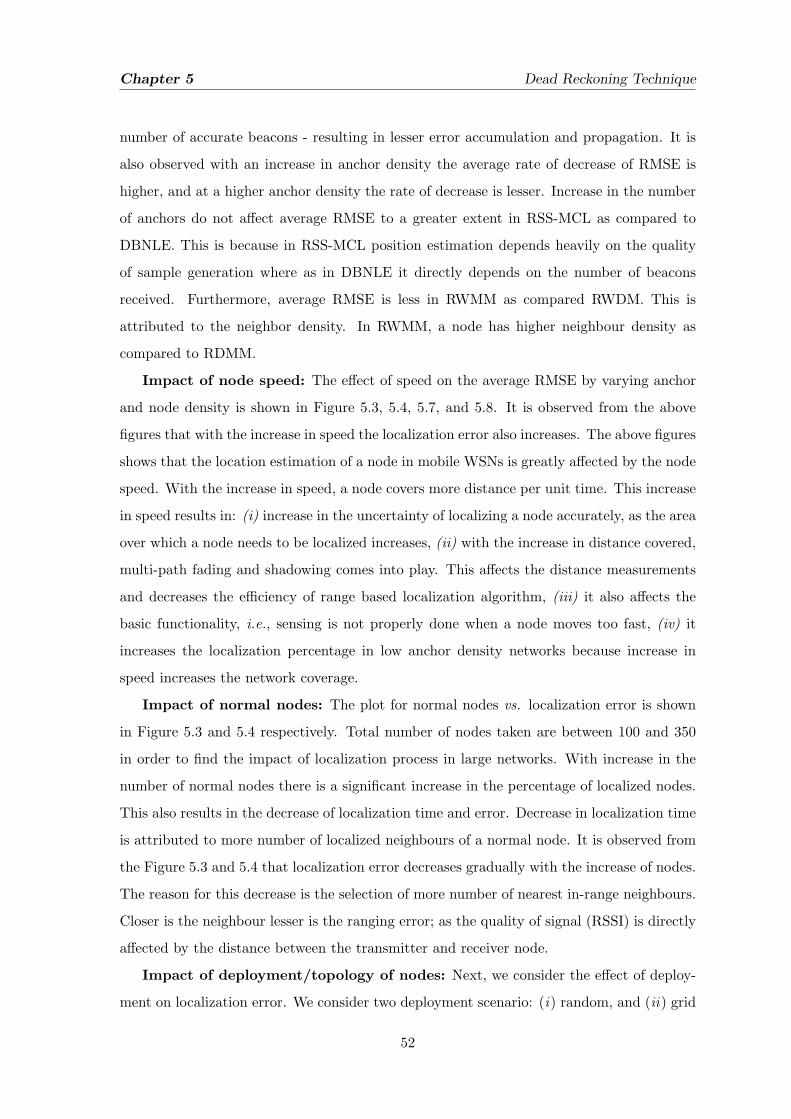
Chapter 5 Dead Reckoning Technique
number of accurate beacons - resulting in lesser error accumulation and propagation. It is
also observed with an increase in anchor density the average rate of decrease of RMSE is
higher, and at a higher anchor density the rate of decrease is lesser. Increase in the number
of anchors do not affect average RMSE to a greater extent in RSS-MCL as compared to
DBNLE. This is because in RSS-MCL position estimation depends heavily on the quality
of sample generation where as in DBNLE it directly depends on the number of beacons
received. Furthermore, average RMSE is less in RWMM as compared RWDM. This is
attributed to the neighbor density. In RWMM, a node has higher neighbour density as
compared to RDMM.
Impact of node speed: The effect of speed on the average RMSE by varying anchor
and node density is shown in Figure 5.3, 5.4, 5.7, and 5.8. It is observed from the above
figures that with the increase in speed the localization error also increases. The above figures
shows that the location estimation of a node in mobile WSNs is greatly affected by the node
speed. With the increase in speed, a node covers more distance per unit time. This increase
in speed results in: (i) increase in the uncertainty of localizing a node accurately, as the area
over which a node needs to be localized increases, (ii) with the increase in distance covered,
multi-path fading and shadowing comes into play. This affects the distance measurements
and decreases the efficiency of range based localization algorithm, (iii) it also affects the
basic functionality, i.e., sensing is not properly done when a node moves too fast, (iv) it
increases the localization percentage in low anchor density networks because increase in
speed increases the network coverage.
Impact of normal nodes: The plot for normal nodes vs. localization error is shown
in Figure 5.3 and 5.4 respectively. Total number of nodes taken are between 100 and 350
in order to find the impact of localization process in large networks. With increase in the
number of normal nodes there is a significant increase in the percentage of localized nodes.
This also results in the decrease of localization time and error. Decrease in localization time
is attributed to more number of localized neighbours of a normal node. It is observed from
the Figure 5.3 and 5.4 that localization error decreases gradually with the increase of nodes.
The reason for this decrease is the selection of more number of nearest in-range neighbours.
Closer is the neighbour lesser is the ranging error; as the quality of signal (RSSI) is directly
affected by the distance between the transmitter and receiver node.
Impact of deployment/topology of nodes: Next, we consider the effect of deploy-
ment on localization error. We consider two deployment scenario: (i) random, and (ii) grid
52
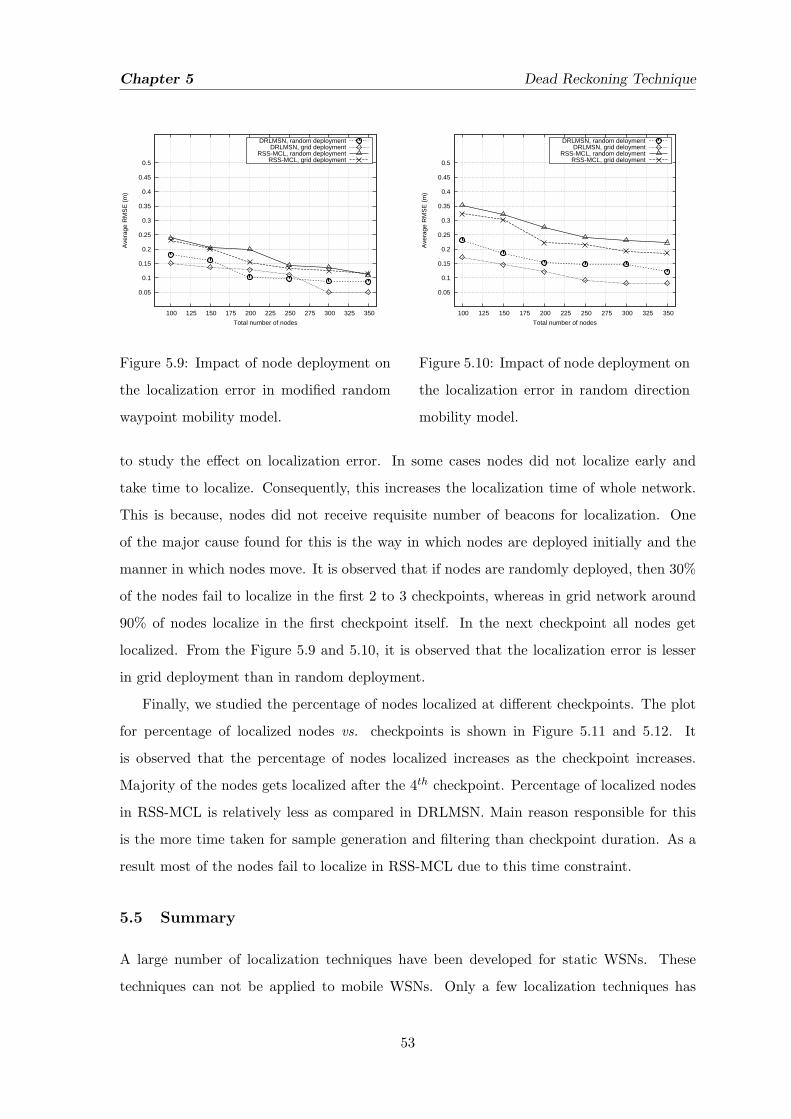
Chapter 5 Dead Reckoning Technique
0.05
0.1
0.15
0.2
0.25
0.3
0.35
0.4
0.45
0.5
100 125 150 175 200 225 250 275 300 325 350
Ave
rage
RM
SE
(m
)
Total number of nodes
DRLMSN, random deploymentDRLMSN, grid deployment
RSS-MCL, random deploymentRSS-MCL, grid deployment
Figure 5.9: Impact of node deployment on
the localization error in modified random
waypoint mobility model.
0.05
0.1
0.15
0.2
0.25
0.3
0.35
0.4
0.45
0.5
100 125 150 175 200 225 250 275 300 325 350
Ave
rage
RM
SE
(m
)
Total number of nodes
DRLMSN, random deloymentDRLMSN, grid deloyment
RSS-MCL, random deloymentRSS-MCL, grid deloyment
Figure 5.10: Impact of node deployment on
the localization error in random direction
mobility model.
to study the effect on localization error. In some cases nodes did not localize early and
take time to localize. Consequently, this increases the localization time of whole network.
This is because, nodes did not receive requisite number of beacons for localization. One
of the major cause found for this is the way in which nodes are deployed initially and the
manner in which nodes move. It is observed that if nodes are randomly deployed, then 30%
of the nodes fail to localize in the first 2 to 3 checkpoints, whereas in grid network around
90% of nodes localize in the first checkpoint itself. In the next checkpoint all nodes get
localized. From the Figure 5.9 and 5.10, it is observed that the localization error is lesser
in grid deployment than in random deployment.
Finally, we studied the percentage of nodes localized at different checkpoints. The plot
for percentage of localized nodes vs. checkpoints is shown in Figure 5.11 and 5.12. It
is observed that the percentage of nodes localized increases as the checkpoint increases.
Majority of the nodes gets localized after the 4th checkpoint. Percentage of localized nodes
in RSS-MCL is relatively less as compared in DRLMSN. Main reason responsible for this
is the more time taken for sample generation and filtering than checkpoint duration. As a
result most of the nodes fail to localize in RSS-MCL due to this time constraint.
5.5 Summary
A large number of localization techniques have been developed for static WSNs. These
techniques can not be applied to mobile WSNs. Only a few localization techniques has
53

Chapter 5 Dead Reckoning Technique
10
20
30
40
50
60
70
80
90
100
1 2 3 4 5 6 7 8
Per
cent
age
of L
ocal
ized
Nod
es
Checkpoints
DRLMSNRSS-MCL
Figure 5.11: Percenatge of localized nodes
at successive checkpoints in modified ran-
dom waypoint mobility model.
10
20
30
40
50
60
70
80
90
100
1 2 3 4 5 6 7 8
Per
cent
age
of L
ocal
ized
Nod
es
Checkpoints
DRLMSNRSS-MCL
Figure 5.12: Percenatge of localized nodes
at successive checkpoints in random direc-
tion mobility model.
been proposed for mobile WSNs. Most of these techniques considered either normal node
or anchor nodes to be static. In this chapter we proposed a localization technique called
dead reckoning for mobile WSN. We have considered both the normal nodes and anchor
nodes to be mobile. As the nodes move in a sensor field, their position changes with time.
Therefore, a mobile node has to be localized as long as it is alive. In the proposed technique,
nodes are localized at discrete time intervals called checkpoint. A normal node is localized
for the first time using three anchor nodes. For subsequent localization it uses only two
anchor nodes and a technique called dead reckoning. Therefore, reducing the number of
anchor nodes required from 3 to 2 at various checkpoints result in: (i) less localization
time, and (ii) lesser localization error as compared to 3 anchor nodes, because more number
of measurements incorporate more inaccurate readings due to multipath and shadowing
effects. We have evaluated the localization error in the proposed scheme by varying the
node density, anchor density, node speed, deployment type and mobility pattern.
In the next chapter, we summarize the contribution made in the thesis. We have also
mentioned the possible future research areas in localization.
54

Chapter 6
Conclusions
Localization in wireless sensor networks have received increasing attention over the last
one decade. It not only provides the geographical position of a sensor node but also fills
the pre-requisite for geographic routing, spatial querying, and data dissemination. With
the continuous research in localization of sensor networks, a number of effective algorithms
have been proposed, but the stability has not yet reached. This is because of the meager
resources (storage, battery, processor) and the harsh deployment environments. Currently,
none of the localization techniques is able to full-fill all these constraints. Most existing
localization algorithms for static WSNs were designed to work with at least three anchor
nodes except in those cases where directional antenna is used. Usage of antenna not only
increases the cost, but also the size of node as well as complexity of the algorithm. As the
number of anchor nodes required in a network increases, overall cost of the network also
increases. In addition, energy drainage of the network increases, but the localization time
of the whole network decreases. Further, anchor nodes installed with GPS do not work well
everywhere. Therefore, at present we are in the need of a novel technology that will solve
the following problems: (i) reduce the number of required anchor nodes, (ii) localize sensor
nodes in areas where GPS do not work well, (iii) minimize the localization error.
In this thesis we have proposed localization technique for static as well as mobile WSNs.
In the reminder of this concluding chapter, we briefly summarize the original contributions
of the study. Finally, some suggestions for future work are given.
6.1 Contribution
Localization Using a Single Anchor Node: First, we proposed a technique for local-
ization, in a grid environment using a single anchor node. It is a distributed, range based
technique. In this technique we classify the nodes into three types. They are: (i) anchor
55

Chapter 6 Conclusions
node, (ii) special node, and (iii) unknown node. Special nodes localize themselves with
respect to anchor node. Unknown node localize with the help of anchor node and special
node. We have compared the proposed scheme with a contemporary scheme called Multi-
duolateration (MDL). We have observed that the localization time and localization error is
smaller in the proposed scheme.
Distributed Binary Node Localization Estimation Approach: It is a distributed,
range based localization algorithm for networks deployed in grid pattern. In this technique
an unknown node is localized using two location aware nodes. This technique is compared
with MDL. It is found that the localization time and localization error is less compared to
MDL.
Dead Reckoning Localization Technique: This technique is proposed for mobile WSNs
while the previous two techniques are for static WSNs. Mobile sensor nodes continuously
change their positions. Therefore, each sensor node needs to be repetitively localized after
certain time interval. This continuously localizing reduces the battery life of sensor nodes.
Furthermore, it is too difficult to localize the mobile sensor nodes accurately as uncertainty
increases with the mobility.
In this technique a node is localized using two anchor nodes. There are two phases
in localization. They are: (i) Initialization phase: In this phase, a node localizes using
trilateration mechanism. Until a node localizes itself using three anchor nodes, it remains
in the initialization phase. (ii) Sequent phase: In this phase a node localizes itself using
only two anchor nodes. Nodes are localized at discrete time interval called checkpoints. A
dead reckoning approach is used to identify the correct estimated position. Once a node is
localized in either of the two phases, it act as settled node and broadcasts a beacon during
the checkpoint.
6.2 Direction for Future Research
Localization problem in WSNs is not yet fully solved. There are several issues in localization
which need further attention. Some of these are below:
(i) Localization accuracy is mostly affected by the ranging techniques used. Each ranging
technique in turn is severely affected by the wireless channel behaviour in different
environments. Therefore, for accurate localization, issues like signal fading, multipath,
additive noise etc needs to be addressed.
56

Chapter 6 Conclusions
(ii) Error in distance measurement between nodes need to be handled with proper cali-
bration because most of localization algorithms depend on the pair-wise distance.
(iii) Not enough work has been drawn on the localization of mobile WSNs. Owing to
more battery drainage in mobile networks, a predictive approach for localization can
estimate the node location with less number of anchors required.
(iv) Monte - Carlo localization (MCL) approach for mobile WSNs needs more attention to
reduce the valid sample generation space. Time required for the generation of valid
samples can be reduced by doing the generation and filtering of samples simultane-
ously.
(v) Localization technique for mobile WSNs needs to be tested in various mobility models.
This ensures that each new proposed technique operate properly in real time networks.
(vi) Furthermore, localization of WSN in certain specific environments like under-water
environments has not been explored much.
57

Bibliography
[1] I. F. Akyildiz, W. Su, Y. Sankarasubramaniam, and E. Cayirci. Wireless Sensor Networks: A
Survey. Computer Networks, 38:393–422, 2002.
[2] P. Juang, H. Oki, Y. Wang, M. Martonosi, Li S. Peh, and D. Rubenstein. Energy-Efficient
Computing for Wildlife Tracking: Design Tradeoffs and Early Experiences with Zebranet. In
Proceedings of the 10th International Conference on Architectural Support for Programming
Languages and Operating Systems, ASPLOS X, pages 96–107, New York, NY, USA, 2002.
ACM.
[3] I. Stojmenovic. Handbook of Sensor Networks : Algorithms and Architectures, chapter 1: In-
troduction to Wireless Sensor Networking, pages 1–34. John Wiley and Sons, first edition,
2005.
[4] I. Mahgoub and M. Ilyas. SMART DUST: Sensor Network Applications, Architecture, and
Design, chapter 1: Opportunities and Challenges in Wireless Sensor Networks, pages 1–13.
Taylor and Francis, first edition, 2006.
[5] A. Pascale, M. Nicoli, F. Deflorio, B. Dalla Chiara, and U. Spagnolini. Wireless Sensor Networks
for Traffic Management and Road Safety. IET Intelligent Transport Systems, 6(1):67–77, 2012.
[6] Dan Li, K. D. Wong, Yu Hen Hu, and A. M. Sayeed. Detection, Classification, and Tracking of
Targets. IEEE Signal Processing Magazine, 19(2):17–29, 2002.
[7] J. G. Ko, C. Lu, M. B. Srivastava, J. A. Stankovic, A. Terzis, and M. Welsh. Wireless Sensor
Networks for Healthcare. Proceedings of the IEEE, 98(11):1947–1960, 2010.
[8] K. Lorincz, D. J. Malan, T. R. F. Fulford-Jones, A. Nawoj, A. Clavel, V. Shnayder, G. Main-
land, M. Welsh, and S. Moulton. Sensor Networks for Emergency Response: Challenges and
Opportunities. IEEE Pervasive Computing, 3(4):16–23, 2004.
[9] L. Buttyan, D. Gessner, A. Hessler, and P. Langendoerfer. Application of Wireless Sensor
Networks in Critical Infrastructure Protection: Challenges and Design Options. IEEE Wireless
Communications, 17(5):44–49, 2010.
[10] J. Zheng and A. Jamalipour. Wireless Sensor Networks A Networking Perspective, chapter 13:
Sensor Network Standards, pages 407–431. John Wiley and Sons, first edition, 2009.
[11] B. Krishnamachari. Networking Wireless Sensors, chapter 4: Time Synchronization, pages
57–68. Cambridge University, first edition, 2005.
58
Bibliography
[12] F. Koushanfar, M. Potkonjak, and A. Sangiovanni-Vincentell. Fault Tolerance Techniques for
Wireless Ad hoc Sensor Networks. In Proceedings of IEEE Sensors, volume 2, pages 1491–1496,
2002.
[13] Y. Liu and Z. Yang. Location, Localization, and Localizability, chapter 7: Localization for
Mobile Networks, pages 97–109. Springer, first edition, 2011.
[14] S. K. Das, J. Wang, R. K. Ghosh, and R. Reiger. Theoretical Aspects of Distributed Computing
in Sensor Networks, chapter 9: Algorithmic Aspects of Sensor Localization, pages 257–259.
Springer, first edition, 2011.
[15] L. Hu and D. Evans. Localization for Mobile Sensor Networks. In Proceedings of the 10th
annual International Conference on Mobile Computing and Networking, MobiCom ’04, pages
45–57, Philadelphia, PA, USA, 2004. ACM.
[16] N. B. Priyantha, A. Chakraborty, and H. Balakrishnan. The Cricket Location-Support System.
In Proceedings of the 6th annual international conference on Mobile computing and networking,
MobiCom ’00, pages 32–43, New York, NY, USA, 2000. ACM.
[17] A. Ward, A. Jones, and A. Hopper. A New Location Technique for The Active Office. IEEE
Personal Communications, 4(5):42–47, 1997.
[18] N. B. Priyantha, Allen K. L. Miu, H. Balakrishnan, and S. Teller. The Cricket Compass for
Context-Aware Mobile Applications. In Proceedings of the 7th annual international conference
on Mobile computing and networking, MobiCom ’01, pages 1–14, New York, NY, USA, 2001.
ACM.
[19] J. Zheng, C. Wua, and Yang Xua Hao Chua. An Improved RSSI Measurement In Wireless
Sensor Networks. Procedia Engineering(Elsevier), 15:876–880, 2011.
[20] D. C. Jenn. Transmission Equation for Multiple Cooperative Transmitters and Collective Beam-
forming. IEEE Antennas and Wireless Propagation Letters, 7:606–608, 2008.
[21] C. Savarese, J. M. Rabaey, and K. Langendoen. Robust Positioning Algorithms for Distributed
Ad-hoc Wireless Sensor Networks. In Proceedings of the General Track of the annual conference
on USENIX Annual Technical Conference, ATEC ’02, pages 317–327, Berkeley, CA, USA, 2002.
USENIX Association.
[22] A. Boukerchie, Horacio A. B. F. Oliveria, E. F. Nakamura, and A. A. F. Loureiro. Localization
Systems For Wireless Sensor Networks. IEEE Wireless Communications, 14(6):6–12, 2007.
[23] L. Kleinrock and J. Silvester. Optimum Transmission Radii for Packet Radio Networks or Why
Six is a Magic Number. In Proceedings of National Telecommunications Conference, volume 1
of NTC ’78, pages 4.3.1–4.3.5, 1978.
[24] R. Nagpal, H. Shrobe, and J. Bachrach. Organizing a Global Coordinate System from Local
Information on an Ad hoc Sensor Network. In Proceedings of the 2nd International Workshop
on Information Processing in Sensor Networks, ISPN 03, Palo Alto, California, April, 2003.
59
Bibliography
[25] I. Stojmenovic. Handbook of Sensor Networks Algorithms and Architectures, chapter 9: Local-
ization in Sensor Networks, pages 277–310. John Wiley and Sons, first edition, 2005.
[26] I. F. Akyildiz and M. C. Vuran. Wireless Sensor Networks, chapter 12: Localization, pages
265–284. John Wiley and Sons Ltd, first edition, 2010.
[27] N. Bulusu, J. Heidemann, and D. Estrin. GPS-less Low-Cost Outdoor Localization for Very
Small Devices. IEEE Personal Communications, 7(5):28–34, Oct. 2000.
[28] X. Li, H. Shi, and Y. Shang. A Partial-Range-Aware Localization Algorithm for Ad-hoc Wireless
Sensor Networks. In Proceedings of the 29th Annual IEEE International Conference on Local
Computer Networks, LCN ’04, pages 77–83, 16–18 Nov. 2004.
[29] Y. Wang, X. Wang, D. Wang, and D. P. Agrawal. Range-Free Localization Using Expected Hop
Progress In Wireless Sensor Networks. IEEE Transactions on Parallel and Distributed Systems,
20(10):1540–1552, Oct. 2009.
[30] T. He, C. Huang, B. Blum, J. Stankovic, and T. Abdelzaher. Range Free Localization Schemes
in Large Scale Sensor Networks. In Proceedings of the 9th annual International Conference on
Mobile Computing and Networking, MobiCom ’03, pages 81–95, 14–19 Sep. 2003.
[31] S. Simic and S. S. Sastry. Distributed Localization in Wireless Ad-hoc Networks. Technical
Report UCB/ERL M02/26, EECS Department, University of California, Berkeley, 2002.
[32] C. Whitehouse. The Design of Calamari: An Ad-hoc Localization System for Sensor Networks.
Technical report, Master’s thesis, University of California, Berkeley, 2002.
[33] J.-P. Sheu, J.-M. Li, and C.-S. Hsu. A Distributed Location Estimating Algorithm for Wireless
Sensor Networks. In IEEE International Conference on Sensor Networks, Ubiquitous, and
Trustworthy Computing, volume 1 of SUTC ’06, pages 218–225, 5–7 June 2006.
[34] J.-P. Sheu, P.-C. Chen, and C.-S. Hsu. A Distributed Localization Scheme for Wireless Sen-
sor Networks with Improved Grid-Scan and Vector-Based Refinement. IEEE Transactions on
Mobile Computing, 7(9):1110–1123, 2008.
[35] Y. Shang, W. Ruml, Y. Zhang, and M. P. J. Fromherz. Localization From Mere Connectivity.
In Proceedings of the 4th ACM international symposium on Mobile Ad-hoc networking and
computing, (MobiHoc ’03), pages 201–212, New York, NY, USA, 1–3 June 2003. ACM.
[36] F. K. W. Chan and H. C. So. Efficient Weighted Multidimensional Scaling For Wireless Sensor
Network Localization. IEEE Transactions on Signal Processing, 57(11):4548–4553, 2009.
[37] S. Zhu and Z. Ding. Bridging Gap Between Multi-dimensional Scaling Based and Optimum
Network Localisation via Efficient Refinement. IET Signal Processing, 6(2):132–142, 2012.
[38] V. Chandrasekhar and W. Seah. An Area Localization Scheme for Underwater Sensor Networks.
In OCEANS ’06, pages 1–8, 16–19 May 2007.
[39] H. M. Khan, S. Olariu, and M. Eltoweissy. Efficient Single-Anchor Localization In Sensor
Networks. In Proceedings Of The Second IEEE Workshop On Dependability and Security in
Sensor Networks and Systems, DSSNS ’06, pages 35–43, 24–28 April 2006.
60

Bibliography
[40] D. Kumar and S. Varma. An Efficient Localization Based On Directional Antenna For Wire-
less Sensor Networks (WSNs). International Journal of Computer and Electrical Engineering,
1(5):542–549, Dec. 2009.
[41] B. Zhang and F. Yu. LSWD: Localization Scheme For Wireless Sensor Networks Using Direc-
tional Antenna. IEEE Transactions on Consumer Electronics, 56(4):2208–2216, Nov. 2010.
[42] U. A. Khan, S. Kar, and J. M. F. Moura. Distributed Sensor Localization In Random Envi-
ronments Using Minimal Number Of Anchor Nodes. IEEE Transactions on Signal Processings,
57(5):2000–2016, May 2009.
[43] H. Lee, Y. Kim, and H. Chong. Grouping Multi-Duolateration Localization Using Partial
Space Information For Indoor Wireless Sensor Networks. IEEE Transactions on Consumer
Electronics, 55(4):1950–1958, 2009.
[44] A. Abramo, F. Blanchini, L. Geretti, and C. Savorgnan. A Mixed Convex/nonconvex Dis-
tributed Localization Approach for the Deployment of Indoor Positioning Services. IEEE Trans-
actions on Mobile Computing, 7(11):1325–1337, 2008.
[45] S. Zhu and Z. Ding. Distributed Cooperative Localization of Wireless Sensor Networks with
Convex Hull Constraint. IEEE Transactions on Wireless Communications, 10(7):2150–2161,
2011.
[46] A. Boulis. Castalia: A simulator for Wireless Sensor Networks and Body Area Networks.
NICTA: National ICT Australia, March 2011.
[47] A. Galstyan, B. Krishnamachari, K. Lerman, and S. Pattem. Distributed Online Localization
in Sensor Networks Using a Moving Target. In Third International Symposium on Information
Processing in Sensor Networks (IPSN), ISPN 04, pages 61–70, 26–27 April 2004.
[48] P. N Pathirana, N. Bulusu, A. V Savkin, and S. Jha. Node Localization Using Mobile Robots
in Delay-Tolerant Sensor Networks. IEEE transactions on Mobile Computing, 4(3):285–296,
May-June 2005.
[49] K.-F. Ssu, C.-H. Ou, and H. C. Jiau. Localization with Mobile Anchor Points in Wireless Sensor
Networks. IEEE transactions on Vehicular Technology, 54(3):1187–1197, May 2005.
[50] J. Jiang, G. Han, H. Xu, Lei Shu, and M. Guizani. LMAT: Localization with a Mobile An-
chor Node Based on Trilateration in Wireless Sensor Networks. In Global Telecommunications
Conference, GLOBECOM ’11, pages 1–6, 5–9 Dec. 2011.
[51] P. Bergamo and G. Mazzimi. Localization in Sensor Networks with Fading and Mobility. In The
13th IEEE International Symposium on Personal, Indoor and Mobile Radio Communications,
volume 2, pages 750–754, 15–18 Sept. 2002.
[52] L. L. de Oliveira, Joao B. Martins, G. Dessbesell, and Jose Monteiro. CentroidM: A Centroid-
based Localization Algorithm for Mobile Sensor Networks. In Proceedings of the 23rd Symposium
on Integrated Circuits and System Design, SBCCI ’10, pages 204–209, New York, NY, USA,
2010. ACM.
61
Bibliography
[53] J.-P. Sheu, W.-K. Hu, and J.-C. Lin. Distributed Localization Scheme for Mobile Sensor Net-
works. IEEE Transactions on Mobile Computing, 9(4):516–526, 2010.
[54] Z. Wang, Y. Wang, M. Ma, and J. Wu. Efficient Localization for Mobile Sensor Networks Based
on Constraint Rules Optimized Monte Carlo Method. Computer Networks, 57(14):2788 – 2801,
2013.
[55] H. J. Rad, A. Amar, and G. Leus. Cooperative Mobile Network Localization via Subspace Track-
ing. In IEEE International Conference on Acoustics, Speech and Signal Processing, ICASSP
’11, pages 2612–2615, 2011.
[56] V. Savic and S. Zazo. Cooperative Localization in Mobile Networks using Nonparametric Vari-
ants of Belief Propagation. Ad Hoc Networks, 11(1):138 – 150, 2013.
[57] M. Nicoli, S. Gezici, Z. Sahinoglu, and H. Wymeersch. Localization in Mobile Wireless and
Sensor Networks. EURASIP Journal on Wireless Communications and Networking, 2011(1):1–
3, 2011.
[58] H. Chen, F. Gao, M. Martins, P. Huang, and J. Liang. Accurate and Efficient Node Localization
for Mobile Sensor Networks. Mobile Networks and Applications, 18(1):141–147, 2013.
[59] S. Tilak, V. Kolar, N. B. Abu-Ghazaleh, and K. D. Kang. Dynamic Localization Control for
Mobile Sensor Networks. In 24th IEEE International Conference on Performance, Computing,
and Communications, IPCC ’05, pages 587–592, 7–9 April 2005.
[60] A. Baggio and K. Langendoen. Monte Carlo Localization for Mobile Wireless Sensor Networks.
Ad Hoc Networks, 6(5):718–733, july 2008.
[61] M. Rudafshani and S. Datta. Localization in Wireless Sensor Networks. In Proceedings of the
6th International Conference on Information Processing in Sensor Networks, ISPN ’07, pages
51–60, Cambridge, Massachusetts, USA, 2007. ACM.
[62] Z. Shigeng, J. Cao, C. Lijun, and C. Daoxu. Locating Nodes in Mobile Sensor Networks More
Accurately and Faster. In 5th Annual IEEE Communications Society Conference on Sensor,
Mesh and Ad Hoc Communications and Networks, SECON ’08, pages 37–45, 16–20 June 2008.
[63] W. D. Wang and Q. X. Zhu. RSS-Based Monte Carlo Localisation for Mobile Sensor Networks.
IET Communications, 2(5):673–681, 2008.
[64] R. R. Roy. Reference Point Group Mobility. In Handbook of Mobile Ad Hoc Networks for
Mobility Models, pages 637–670. Springer US, 2011.
[65] C. Schindelhauer. Mobility in Wireless Networks. In Proceedings of the 32nd Annual Conference
on Current Trends in Theory and Practice of Computer Science, SOFSEM ’06, pages 100–116,
Berlin, Heidelberg, 2006. Springer-Verlag.
[66] E. M. Royer, P. Michael Melliar-Smithy, and L. E. Moser. An Analysis of the Optimum Node
Density for Ad hoc Mobile Networks. In IEEE International conference on Communications,
ICC, volume 3, pages 857–861, 2001.
62