local regression-based short-term load forecasting

Journal of Intelligent and Robotic Systems 31: 115–127, 2001.© 2001 Kluwer Academic Publishers. Printed in the Netherlands.

115

Local Regression-Based Short-Term LoadForecasting

RASTKO ZIVANOVICTechnikon Pretoria, South Africa; e-mail: [email protected]

(Received: 6 February 2000; accepted: 20 June 2000)

Abstract. This paper presents a novel method for short-term load forecasting based on local poly-nomial regression. Before applying the local regression, data mining algorithm selects historic loadsequences satisfying known factors that are characterising required load model. Further on, theselected sequences are pre-processed with robust location estimator (M-estimator) in order to re-duce serial correlation and to eliminate outliers in historic data. On pre-processed load data weapplied locally a truncated Taylor expansion to approximate functional relationship between loadand load-affecting factors. Two methods for selecting optimal smoothing parameters (window sizeand polynomial degree) for local approximations are presented in the paper. These algorithms offerto us close insight into trade-off between bias and variance of the local approximations. In that way,they are able to help in selecting smoothing parameters locally (for each local fit) to fulfil the loadmodelling requirements. An example is presented at the end of this paper that clearly demonstratesthe main features of this method.

Key words: short-term load forecasting, local polynomial regression, locally adaptive models, non-parametric statistics, forecasting, power systems.

1. Introduction

Short-term load forecasting is one of the most important functions in today’s mod-ern energy management systems used in electricity utilities worldwide. It is typ-ically providing hourly forecasts for one day to one week ahead. Hourly loadforecasts are used to establish operational plans for power plants and interchangeschedules with neighbouring utilities. Accuracy of a short-term load forecastingmethod has direct impact on overall financial performance of a utility.

The various methods are developed for short-term load forecasting (Gross andGaliana, 1987; Liu et al., 1995). They could be classified in one of the two broadcategories: parametric and nonparametric. The parametric methods assume that aload model has some pre-specified functional form. This functional form repre-senting quantitative relationships between load and load affecting factors is de-fined through exploratory statistical research of the available historical data. Theseparametric models are developed either in time domain or in frequency domain(Liu et al., 1995). The assumed function parameters are then estimated from histori-cal data and the adequacy of the model checked using classical statistical diagnostic

116 R. ZIVANOVIC

procedures. The serious problem in using parametric approach is the need forrather elaborate models (for example, polynomials with higher degree). This willlead ultimately to inefficient smoothing of historical data with the forecasts havinglarge variance. Another problem is that the model developed through exploratoryresearch is data dependent and it will not perform well in another electricity util-ity.

As an alternative, in the nonparametric approach one tries to formulate loadmodel without reference to a specific function and associated set of parameters.Methods using artificial neural networks belong to the nonparametric category(Park et al., 1991). They have ability to learn the relationship load–load-affectingfactors from historic data without necessity of pre-specifying an appropriate func-tional form. The well-known problem is how to select the optimal structure of anetwork to secure an acceptable forecast accuracy. For example, a network withtoo many hidden neurones will memorize training data instead of learning generalrelationships. With too many neurones we increase variance of the forecasts. Sucha network will perform badly for data outside training set. In the same way, if wetry to reduce the variance by constraining the network to have a limited number ofparameters, we will increase bias of the forecasts. The optimal solution will be acompromise between bias and variance. To find the optimal solution in short-termload forecasting problem we propose local regression method.

The main goal of this paper is to present the application of local (nonparametric)modelling techniques in short-term load forecasting. Load modelling methodologyexplained in the second section of this paper builds upon existing data miningalgorithm for retrieval daily load sequences that are matching specific require-ments (Graupe and Zivanovic, 1999). Errors inside each selected load sequenceare serially correlated but they are independent across matched days. To reducethis correlation and eliminate outliers use of a robust M-estimator is proposed(Huber, 1981). Furthermore, we derived a load-modelling approach based on localregression (Katkovnik, 1985), and methods for estimating local bias and variance.In this approach, instead of solving a parametric problem with many parameterswe solve many local linear or low order polynomial-fitting problems. In the thirdsection, we introduced two criteria for selecting smoothing parameters (polynomialdegree and window size) locally (Cleveland and Loader, 1996; Goldenshlunger andNemirovski, 1997; Katkovnik, 1998). In these algorithms, the size of local neigh-bourhood (window) or local polynomial degree for each fitted point are chosen bydata, to balance between bias and variance in load forecasts. Some of the results inapplying nonparametric regression in short-term load forecasting are presented inthe Section 4.

2. Load Model

Factors influencing pattern of a daily load variation could be classified as calendarvariables (hour, season, day of the week, holiday indicator, and weekend indica-

LOCAL SHORT-TERM LOAD FORECASTING 117

tor), weather variables (temperature, humidity, wind speed, cloud cover, etc.) andsystem variables (electricity price and other electricity market related information).However, in practice, one has to relay on the variables that are ultimately availableand on those, which could be forecasted with high accuracy. We assume the avail-ability of the historic database consisting of daily load-temperature sequences andforecasted tomorrow’s minimal and maximal temperatures (Graupe and Zivanovic,1999).

2.1. HISTORY MATCHING

In the first phase, the historic database is searched for daily load sequences that arematching specific requirements for designing tomorrow’s load model. Calendarvariables and tomorrow’s forecasted minimal and maximal temperatures specifythese requirements. The searching criteria and all results are accessible in an inter-active manner to accommodate the experience of utility load planner to foresee theeffects of some load affecting factors, not taking into consideration in automaticload modelling (Graupe and Zivanovic, 1999). The final result of the search is theset of hourly load sequences for matched days. Each set is extended with loadsfrom days before and after the matched day, to eliminate boundary effects in localregression with symmetrical sliding window.

We assume the following model for a collection of historic load-time series:

Pij = m(i) + εij , i = 1, . . . , Nh, j = 1, . . . , Nd, (2.1)

where Nh > 24 is the number of hourly load values in each extended load se-quence, and Nd is the number of matched days. m is an unknown function andεij is an error term, representing random errors and variability from sources notincluded in the model. The errors are zero mean random variables satisfying

cov(εij , εkl) ={σ 2ρ(i − k) if j = l,0 if j �= l,

(2.2)

where ρ is the correlation function with ρ(0) = 1 and |ρ(u)| � 1 for all u ∈[−1, 1]. As could be deduced from (2.1) and (2.2), this model assumes serial de-pendence structure. Errors inside each load sequence are correlated but they areindependent across the matched days. To reduce this correlation we formulate themodel based on averaged responses as

Pi = m(i) + εi, i = 1, . . . , Nh, (2.3)

where

Pi = 1

Nd

Nd∑j=1

Pij . (2.4)

Now the averaged errors εi satisfy

cov(εi, εk) = σ 2

Nd

ρ(i − k). (2.5)

118 R. ZIVANOVIC

In this way the requirement for independent errors, which is needed in local regres-sion later, could be satisfied. The estimation of m is the problem of fitting a smoothcurve through mean values at each hour.

We must be aware that the mean (2.4) can be upset completely by outliersamong the load values across matched days. Reasons to have these unexpectedload sequences could be outage of some loads due to faults in a system, or holidaysthat we did not exclude in the search. To guard against outliers robust methods haveto be used. Instead of the simple mean (2.4) we used M-estimator (Huber, 1981),defined as

minPi

Nd∑j=1

f (Pij − Pi). (2.6)

For example, the mean (2.4) corresponds to f (r)= r2 and the median to f (r)= |r|.Let ψ = f ′, then Pi is the estimator obtained by solving

∑Nd

j=1 ψ(Pij − Pi) = 0using iterative method. The function we used levels the outliers to Pi ± c,

ψ(r) ={−c if r < −c,r if |r| < c,c if r > c,

(2.7)

where c = 1.345 for 95% efficiency at the normal distribution. Robust standarddeviation estimate for an hour i is based on median absolute residuals

σi = 1.4826 × medianj

∣∣Pij − medianj

(Pij )∣∣, (2.8)

where factor 1.4826 is chosen when the Pij values are normally distributed (ex-cluding outliers). Furthermore, we need to use standard deviation (2.8) to scaleresiduals in (2.6) before we estimate Pi . The estimate (2.8) will be used later inlocal regression procedure, to account for nonhomogeneous variance of historicload data.

It should be noted that we could impose additional weight sequence when weevaluate the means (2.4) or the robust estimates (2.6). To put more weight to recentobservations than on older ones (weights decreasing with age), leads to exponentialsmoothing (Graupe and Zivanovic, 1999).

2.2. LOCAL POLYNOMIAL REGRESSION

We assume that locally around an hour t , the function m in the model (2.3) canbe approximated with a class of polynomial functions. If p derivatives of thefunction m at t exist, we can apply a truncated Taylor’s series expansion (up to theorder p) around point t . It follows that the function at point u (in the neighbourhoodof t) could be approximated by

m(u)≈m(t)+m′(t)(u− t)+ m′′(t)2! (u− t)2 + · · · + m(p)(t)

p! (u− t)p. (2.9)


The neighbourhood (sliding window) is determined with a bandwidth parameterh > 0. In this application the symmetric window centred at t will be used: (t −h, t + h). In some signal processing applications the nonsymmetric window (one-sided smoothing) could be more appropriate (Zivanovic, 1999). To approximatem(u), only observations within this window are used.

It should be noted that the explanatory variables are equally spaced points(hours), and therefore for the window centred at t the Taylor’s series (2.9) is ofthe form:

m(t + k − h) ≈p∑

i=0

Ci(t)(k − h)i, (2.10)

where Ci(t) = m(i)(t)/i!, and k goes from 0 to n = 2h. The coefficients Ci can beestimated by minimising locally weighted sum of squares:

1

n + 1

n∑k=0

1

σ 2k

w

(k − h

h

)[Pk −

p∑i=0

Ci(t)(k − h)i

]2

, (2.11)

where σk is the standard deviation estimate for Pk , obtained from (2.8). The squaredresiduals in (2.11) are additionally weighted with w((k−h)/h) function accordingto the distance from t . The simplest choice for the weight function is the rectangularfunction, but it is rarely used, since it could leads to a discontinuous fitted curve.Usually, the weight function is chosen to be continuous, symmetric, with the peakat 0 (it assigns the largest weight to the residual at t) and supported on the interval[−1, 1]. In this application we going to use the tricube weight function

w(u) = (1 − |u|3)3

, |u| < 1. (2.12)

The weighted least square solution of (2.11) is given by

c = (ATVWA

)−1ATWVP, (2.13)

where

c = [C0, C1, . . . , Cp]T is the (p + 1) coefficient vector;

P =[P0, . . . , Pn]T is the (n+ 1) vector of loads spanning the sliding win-

dow;

W = diag

[w(−1), w

(1 − h

h

), . . . , w(0), . . . , w

(h − 1

h

), w(1)

]and

V = diag

[1

σ 20

1

σ 21

. . .1

σ 2n

]

120 R. ZIVANOVIC

are the (n + 1) × (n + 1) diagonal weight matrices; and

A =

1 (−h) (−h)2 . . . (−h)p

1 (1 − h) (1 − h)2 . . . (1 − h)p

......

...

1 0 0 0...

......

1 h h2 . . . hp

is the (n + 1) × (p + 1) design matrix.

Now, when we know the polynomial coefficients (2.13), local estimate of theload function at hour t is obtained by setting k = h in (2.10)

m(t) = C0. (2.14)

The result (2.14) can be represented in the linear estimator form by using equiva-lent weights lk(p, h), which are the function of polynomial degree (p) and band-width (h)

m(t) =n∑

k=0

lk(p, h)Pk. (2.15)

The vector of equivalent weights l(p, h) = {li(p, h)}ni=0 is obtained from (2.13)

l(p, h)T = eT1

(ATVWA

)−1ATWV, (2.16)

where e1 is the unit vector: e1 = [1 0 . . . 0]T. It should be noted that the ex-pression (2.16) could be reduced to simple formulas for calculating each equivalentweight for given k, h, and p. The standard deviations for each Pk could be includedin these formulas, as in (2.16), to account for nonhomogenous variance. In the sim-plified case of uncorrelated errors with homogenous variance in the model (2.3),the equivalent weights would have the following important property

n∑k=0

lk(p, h)(k − h)j ={

1 if j = 0,0 if 1 � j � p.

(2.17)

This property, as we going to demonstrate later, has a direct effect on bias reductionin load modelling based on local regression. For example, bias of a local linearmodel would not depend on the slope of underlining load function.

2.3. LOCAL BIAS AND VARIANCE

To have a good insight into bias and variance of the linear estimator (2.15) isan essential issue in understanding the influence of polynomial degree and band-width on accuracy of the local regression modelling. A nice feature of the linear


estimator (2.15) is that it reveals simple expressions for estimators of local biasand variance. These expressions are derived assuming uncorrelated errors withhomogenous variance. The conclusions drown from these expressions could beused as valuable guidance in more general case, for errors having nonhomogenousvariance.

The local bias of the linear estimate (2.15) at point t is equal to

E(m(t)

)− m(t) = E

[n∑

k=0

lk(p, h)(m(t + k − h) + εk

)]− m(t). (2.18)

Assuming that m(t) is p + 1 times differentiable, we can expand m(t) in a Taylorseries around t in a same way as in (2.9), and use it in (2.18),

E(m(t)

)− m(t)

= E

[n∑

k=0

lk(p, h)

(p+1∑i=0

m(i)(t)

i! (k − h)i + εk

)]− m(t). (2.19)

An application of the property (2.17) leads to the expression for bias:

E(m(t)

)− m(t) = b(p, h)m(p+1)(t), (2.20)

where

b(p, h) = 1

(p + 1)!n∑

k=0

lk(p, h)(k − h)p+1

is the bias factor that measures the bias change in function of polynomial degree p

and sliding window size (bandwidth h). The expression for local variance at t isderived in a similar way,

var(m(t)

) = σ 2∥∥l(p, h)∥∥2

, (2.21)

where ‖l(p, h)‖2 = ∑nk=0 lk(p, h)

2 is the variance factor that measures the vari-ance change in function of polynomial degree p and sliding window size (band-width h).

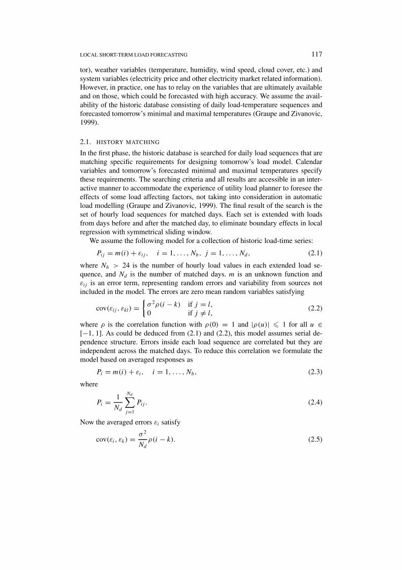
The bias factor (biasn = b(p, h)) and the square root of variance factor (stdn =‖l(p, h)‖) in function of polynomial degree p and sliding window size (2h + 1)are shown in Figure 1.

By analyzing the Figure 1 as well as the expressions for bias and variance,(2.20) and (2.21), we deduce the following important conclusions about influenceof smoothing parameters on local load modeling:(a) bias of a model increases with the p + 1 derivative of the function m when a

polynomial of order p is used;(b) for small window size, the effects of increasing polynomial order (p) are the

bias reduction and increase of the variance;

122 R. ZIVANOVIC

Figure 1. The bias and standard deviation factors in function of p and 2h + 1.

(c) for large window size, by increasing polynomial order (p) the bias will in-crease and the variance will increase.

(d) by increasing the window size for given p variance can be reduced but at thesame time bias will increase.

Based on the above observations one optimal strategy is to keep polynomialorder low (p = 1, for example) and change window size. Maximize the sizefor flat (smooth) regions of the function (p + 1 derivative low) and reduce thesize for the uneven regions (p + 1 derivative high). From the other side, if vari-ability is low and we use small constant bandwidths, it makes sense to increasepolynomial degree, and in that way reduce bias of a model at places with highcurvature.

3. Smoothing Parameters Selection

It has been noticed that load curves have a large amount of structure and that nota single bandwidth or local polynomial degree will produce an adequate fit to alldata. Therefore, we decided to vary locally smoothing parameters (p and h). In thatway we can obtain satisfactory fit for load curve peaks and smoother parts. To findthe best smoothing parameters one needs to solve local regression problems severaltimes. The computationally efficient way of calculating many smooth functions is


based on transformation of the linear estimation equation (2.15) into frequencydomain (Haerdle, 1987). The efficiency comes from decoupling the smoothingoperation from the Fourier transform of the load data (computed via FFT). Forcomputing several local regression functions the rescaled Fourier transform of theequivalent weight vector (2.16) has to be multiplied with Fourier transform of theload data. Each candidate fit should be assessed locally to select the best localfit. The assessment is based on either local goodness of fit measure (we used CPstatistic (Cleveland and Loader, 1996)) or on Intersection of Confidence Intervals(ICI) method (Katkovnik, 1998).

3.1. LOCAL CP STATISTIC

For a fixed point t , consider a local polynomial fit using degree p and bandwidth h.The coefficients c of the fitted polynomial are computed using weighted leastsquares method, as in (2.13) where nonhomogenous variance is allowed. This localpolynomial is evaluated at the data point k − h, as

m(t + k − h) =p∑

i=0

Ci(k − h)i . (3.1)

The local goodness of fit measure is defined as weighted sum of the squared errorsover a local window of size n + 1,

Jt =∑n

k=0(1/σ2k )w((k − h)/h)[m(t + k − h) − m(t + k − h)]2∑n

k=0 w((k − h)/h). (3.2)

The expected value of (3.2) can be decomposed into bias and variance. The un-known bias is replaced with residual sum of squares plus the corresponding vari-ance term, leading to the CP expression for calculating unbiased estimate of thelocal goodness of fit (Cleveland and Loader, 1996)

CPt = 1

tr(W)

n∑k=0

1

σ 2k

w

(k − h

h

)[Pk − m(t + k − h)

]2 + 2ν(m)

tr(W)− 1, (3.3)

where ν(m) is a local fitted degrees of freedom,

ν(m) = tr[(

ATWVA)−1

ATW2VA], (3.4)

and A, W, V are defined in (2.13).

3.2. INTERSECTION OF CONFIDENCE INTERVALS

The Intersection of Confidence Intervals (ICI) method is suitable in finding optimalsize of local window (bandwidth) for given local polynomial degree. For a local

124 R. ZIVANOVIC

model estimate mh(t), computed with bandwidth h at point t , a confidence intervalfor the mean has the form

Dh(t) = [mh(t) − κ

∥∥l(p, h)∥∥, mh(t) + κ∥∥l(p, h)∥∥], (3.5)

where choosing κ = 1.96 leads to 95% confidence interval under normality as-sumption, and l(p, h) is calculated according to (2.16). As we discussed in Sec-tion 2.3, by increasing the window size the variance factor ‖l(p, h)‖ and standarddeviation of mh(t) will decrease. This makes the confidence interval (3.5) narrower.If we make the window too large, the estimate becomes biased. The balance be-tween bias and variance makes goodness of fit measure (3.2) the smallest. Thisis obtained for the bandwidth h∗ such that the set

⋂h1�h�h∗ Dh(t) is nonempty

(Goldenshlunger and Nemirovski, 1997; Katkovnik, 1998).

4. Example

The proposed method was tested using two years of historic records of hourlyload and temperature (Graupe and Zivanovic, 1999). In the first phase, forecastsfor tomorrow’s minimal and maximal temperatures, day of the week, and seasonindicator are used as inputs in the searching algorithm (Graupe and Zivanovic,1999). The result was a selection of 38 similar days. We did not exclude holidaydays in this search and therefore the algorithm selected 6 of them. Figure 2 plotsthese selected loads for each hour (as dots) plus two lines: the upper one representsthe robust location estimator (2.6) and the one beneath represents the mean (2.4).The holiday load curves are clearly outliers (dots far below main data cloud) andtherefore the robust location estimator gives more reliable estimate compared tothe mean. The load sequences selected in the search process (shown in the middleof Figure 2) are extended with day before and day after sequences.

In the second phase we have a choice of two strategies in selecting smoothingparameters. Either to vary polynomial order or window size. The upper panel ofFigure 3 shows the forecast when the sliding window size is fixed to 8 and poly-nomial degree (1, 2 or 3) is selected using local CP statistic (3.3). In the lowerpanel the selected degrees for each fitted point are shown. In the parts with highvariability and small load change (from 11 h till 20 h) the algorithm selected locallinear fits. This reduces variance of load forecast. Around the afternoon peak (highcurvature) and parts with low variance and sharp change (from 22 h till 10 h in themorning), local quadratic and cubic fits are preferred. This clearly reduces bias ofthe load model. The actual load (dashed line) and robust location estimates (circles)are plotted in the same figure for comparison.

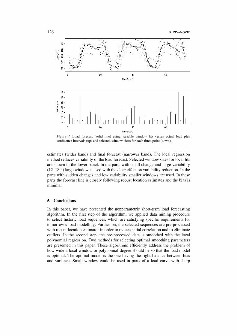
The second choice is to keep constant polynomial degree and change the win-dow size. We applied in this example local linear fit with ICI algorithm for windowsize selection. The upper panel of Figure 4 presents the forecasted load versusthe actual load (dashed line) and robust location estimates (circles). In this fig-ure (using dotted lines) we added 95% confidence intervals for robust location


Figure 2. The selected daily load sequences (dots) with the mean (lower line) and the robustlocation estimate (upper line).

Figure 3. Load forecast (solid line) using variable order fit versus actual load (up) and selectedpolynomial degrees (down).

126 R. ZIVANOVIC

Figure 4. Load forecast (solid line) using variable window fits versus actual load plusconfidence intervals (up) and selected window sizes for each fitted point (down).

estimates (wider band) and final forecast (narrower band). The local regressionmethod reduces variability of the load forecast. Selected window sizes for local fitsare shown in the lower panel. In the parts with small change and large variability(12–18 h) large window is used with the clear effect on variability reduction. In theparts with sudden changes and low variability smaller windows are used. In theseparts the forecast line is closely following robust location estimates and the bias isminimal.

5. Conclusions

In this paper, we have presented the nonparametric short-term load forecastingalgorithm. In the first step of the algorithm, we applied data mining procedureto select historic load sequences, which are satisfying specific requirements fortomorrow’s load modelling. Further on, the selected sequences are pre-processedwith robust location estimator in order to reduce serial correlation and to eliminateoutliers. In the second step, the pre-processed data is smoothed with the localpolynomial regression. Two methods for selecting optimal smoothing parametersare presented in this paper. These algorithms efficiently address the problem ofhow wide a local window or polynomial degree should be so that the load modelis optimal. The optimal model is the one having the right balance between biasand variance. Small window could be used in parts of a load curve with sharp


change and low variability. On the other hand, large window is suitable for moresteady parts of the load curve with large variability. It will reduce variance. Inthe parts with high curvature (like afternoon peak in our example) we could usesmall window and increase polynomial degree. This will reduce bias on daily loadpeak forecast, which is of utmost importance for electricity utilities. In general,the methods for selecting smoothing parameters could be used to adapt locallyload model for a specific situation and requirements. In this way, as shown in ourexample, we are able to achieve the best trade-off between bias and variance in allparts of a tomorrow’s load model.

References

Cleveland, W. S. and Loader, C. R.: 1996, Smoothing by local regression: Principles and meth-ods, in: W. Haerdle and M.G. Schimek (eds), Statistical Theory and Computational Aspects ofSmoothing, Heidelberg, Physica-Verlag, pp. 10–49.

Gross, G. and Galiana, F. D.: 1987, Short-term load forecasting, Proc. IEEE 75(12), 1558–1572.Graupe, W. and Zivanovic, R.: 1999, An overview of the short-term load forecasting methodology in

NamPower, in: Universities Power Engineering Conference, Leicester, England.Goldenshlunger, A. and Nemirovski, A.: 1997, On spatial adaptive estimation of nonparametric

regression, Math. Methods Statist. 6, 135–170.Huber, P. J.: 1981, Robust Statistics, Wiley, New York.Haerdle, W.: 1987, Resistant smoothing using the fast fourier transform, Appl. Statist. 36, 104–111.Katkovnik, V. Y.: 1985, Nonparametric Identification and Smoothing of Data: Local Approximation

Method, Nauka, Moscow.Katkovnik, V. Y.: 1998, On multiple window local polynomial approximation with varying adaptive

bandwidths, in: COMPSTAT 1998, Proceedings in Computational Statistics, Physica-Verlag,pp. 353–358.

Liu, K. et al.: 1995, Comparison of short-term load forecasting techniques, in: IEEE PES ’95 SummerMeeting, paper 95 SM 547-0 PWRS.

Park, D. et al.: 1991, Electric load forecasting using an artificial neural network, IEEE Trans. PowerSystems 6(2), 442–449.

Zivanovic, R.: 1999, Frequency estimation algorithm based on local polynomial approximation, in:Universities Power Engineering Conference, Leicester, England.

local regression-based short-term load forecasting

Documents