local oscillations in finite difference solutions of ... · local oscillations in finite di erence...
TRANSCRIPT

Local Oscillations in Finite Difference Solutions
of Hyperbolic Conservation Laws
Huazhong Tang
School of Mathematical Sciences
Peking University
Beijing 100871, P.R. China
Website: dsec.pku.edu.cn/∼tanghz
Joint work with Jiequan Li & Lumei Zhang (Capital Normal
University, China)
Gerald Warnecke (Otto-von-Guericke-Universitat of Magdeburg,
Germany)

Outline
1 Motivation
2 Chequerboard modes in the initial discretization
3 Propagation of the chequerboard mode
4 Discrete Fourier analysis
5 Modified equation analysis
6 Conclusions

Outline
1 Motivation
2 Chequerboard modes in the initial discretization
3 Propagation of the chequerboard mode
4 Discrete Fourier analysis
5 Modified equation analysis
6 Conclusions

Motivation
-0.25
-0.2
-0.15
-0.1
-0.05
0
0.05
0.1
0.15
0.2
-4 -3 -2 -1 0 1 2 3 4
u
x
-0.15
-0.1
-0.05
0
0.05
0.1
0.15
0.2
-4 -3 -2 -1 0 1 2 3 4
u
x
-0.1
-0.08
-0.06
-0.04
-0.02
0
0.02
0.04
0.06
0.08
0.1
-4 -3 -2 -1 0 1 2 3 4
u
x
Figure: Numerical solutions of IVP of the linear advection equation
ut + 0.2ux = 0 by MONOTONE schemes [H.Z. Tang & G. Warnecke,
M2AN, 38 (2004)].
• Why does the monotone scheme produce local
/counterintuitive oscillations?

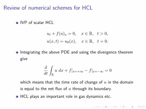
Review of numerical schemes for HCL
IVP of scalar HCL
ut + f(u)x = 0, x ∈ R, t > 0,
u(x, t) = u0(x), x ∈ R, t = 0.
Integrating the above PDE and using the divergence theorem
give
d
dt
∫Ru dx+ f |x=+∞ − f |x=−∞ = 0
which means that the time rate of change of u in the domain
is equal to the net flux of u through its boundary.
HCL plays an important role in gas dynamics etc.

Review of numerical schemes for HCL
Lax-Wendroff theorem [CPAM, 1960]: If the solutions of the
conservative scheme converge to a function u as
max{τ, h} → 0, then u is a weak solution of HCL.
Conservative scheme in the viscous form
un+1j =unj −
ν
2
(f(unj+1)− f(unj−1)
)+Qnj+1/2
2(unj+1 − unj )
−Qnj−1/2
2(unj − unj−1),
where ν = τ/h, and τ & h are time and space step sizes,
respectively.
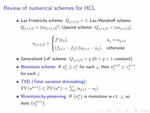
Review of numerical schemes for HCL
Lax-Friedrichs scheme: Qj+1/2 = 1; Lax-Wendroff scheme:
Qj+1/2 = |νaj+1/2|2; Upwind scheme: Qj+1/2 = |νaj+1/2|.
aj+1/2 =
f ′(uj), uj = uj+1
(fj+1 − fj)/(uj+1 − uj), otherwise.
Generalized LxF scheme: Qj+1/2 = q (0 < q < 1 constant)
Monotone scheme: If unj ≥ vnj for each j, then un+1j ≥ vn+1
j
for each j.
TVD (Total variation diminishing):
TV (un+1) ≤ TV (un) :=∑
j |uj+1 − uj |.
Monotonicity-preserving: If {unj } is monotone w.r.t. j, so
does {un+1j }.
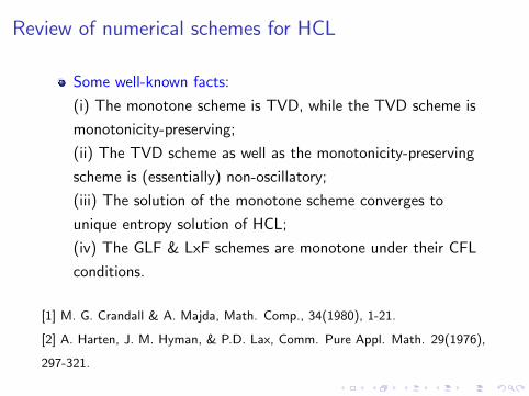
Review of numerical schemes for HCL
Some well-known facts:
(i) The monotone scheme is TVD, while the TVD scheme is
monotonicity-preserving;
(ii) The TVD scheme as well as the monotonicity-preserving
scheme is (essentially) non-oscillatory;
(iii) The solution of the monotone scheme converges to
unique entropy solution of HCL;
(iv) The GLF & LxF schemes are monotone under their CFL
conditions.
[1] M. G. Crandall & A. Majda, Math. Comp., 34(1980), 1-21.
[2] A. Harten, J. M. Hyman, & P.D. Lax, Comm. Pure Appl. Math. 29(1976),
297-321.

Review of numerical schemes for HCL
-1
-0.5
0
0.5
1
1.5
2
-1 -0.5 0 0.5 1 1.5 2
u
x
-1
-0.5
0
0.5
1
1.5
-1 -0.5 0 0.5 1 1.5 2
u
x
-1
-0.5
0
0.5
1
1.5
-1 -0.5 0 0.5 1 1.5 2
u
x
Figure: Numerical results for the linear advection equation ut + ux = 0.
From left to right: 2nd order LW, 1st order upwind, and 2nd order TVD.
• The LW scheme is 2nd order accurate in time and space,
and not monotone & TVD as well as
monotonicity-preserving, thus produces numerical
oscillations.

Glimpse of local oscillations in the GLF scheme
Consider the generalized LxF schemes (GLF)
un+1j = unj −
ν
2
(f(unj+1)− f(unj−1)
)+q
2(unj+1− 2unj + unj−1), (1)
and understand local oscillations in solutions of (1) by Fourier
analysis and modified equation methods, even though GLF is
monotone and TVD under a certain restriction.
A glimpse: Taking the highest frequency mode, a chequerboard
mode, as the initial data, then we have the solution of GLF (1)
unj = (1− 2q)n(−1)j .
It shows that the solution of (1) is still a chequerboard mode,
except for the modified LxF scheme with q = 1/2. The amplitude
of the solution is diminishing if 0 < q < 1 but keeps invariant for
the LxF scheme with q = 1 or for the unstable central scheme with
q = 0.
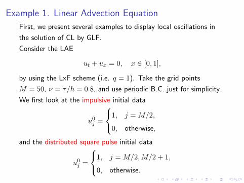
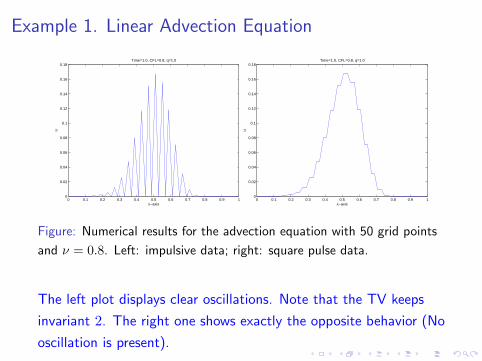
Example 1. Linear Advection Equation
First, we present several examples to display local oscillations in
the solution of CL by GLF.
Consider the LAE
ut + ux = 0, x ∈ [0, 1],
by using the LxF scheme (i.e. q = 1). Take the grid points
M = 50, ν = τ/h = 0.8, and use periodic B.C. just for simplicity.
We first look at the impulsive initial data
u0j =
1, j = M/2,
0, otherwise,
and the distributed square pulse initial data
u0j =
1, j = M/2,M/2 + 1,
0, otherwise.
Example 1. Linear Advection Equation
0 0.1 0.2 0.3 0.4 0.5 0.6 0.7 0.8 0.9 10
0.02
0.04
0.06
0.08
0.1
0.12
0.14
0.16
0.18
x−axis
uTime=1.0, CFL=0.8, q=1.0
0 0.1 0.2 0.3 0.4 0.5 0.6 0.7 0.8 0.9 10
0.02
0.04
0.06
0.08
0.1
0.12
0.14
0.16
0.18
x−axis
u
Time=1.0, CFL=0.8, q=1.0
Figure: Numerical results for the advection equation with 50 grid points
and ν = 0.8. Left: impulsive data; right: square pulse data.
The left plot displays clear oscillations. Note that the TV keeps
invariant 2. The right one shows exactly the opposite behavior (No
oscillation is present).

Example 2. Burgers equation ut + (u2/2)x = 0
0 0.1 0.2 0.3 0.4 0.5 0.6 0.7 0.8 0.9 10
0.02
0.04
0.06
0.08
0.1
0.12
0.14
0.16
0.18
x−axis
u
Time=1.0, CFL=0.8, q=1.0
0 0.1 0.2 0.3 0.4 0.5 0.6 0.7 0.8 0.9 10
0.02
0.04
0.06
0.08
0.1
0.12
0.14
0.16
0.18
x−axis
u
Time=1.0, CFL=0.8, q=1.0
Figure: Same as the last figure except for the Burgers equation. Left:
impulsive data; right: square pulse data.
Similar numerical phenomena are observed. Therefore, the
oscillations are not connected to the nonlinearity, just for
chequerboard mode.
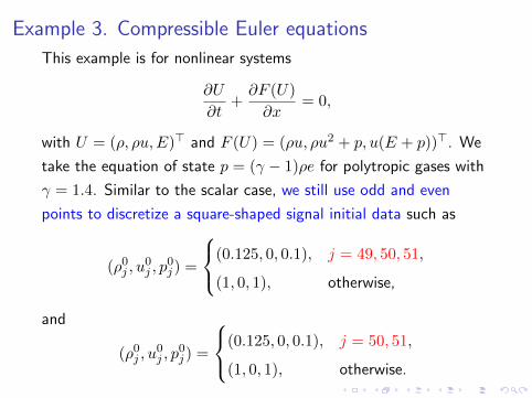
Example 3. Compressible Euler equations
This example is for nonlinear systems
∂U
∂t+∂F (U)
∂x= 0,
with U = (ρ, ρu,E)> and F (U) = (ρu, ρu2 + p, u(E + p))>. We
take the equation of state p = (γ − 1)ρe for polytropic gases with
γ = 1.4. Similar to the scalar case, we still use odd and even
points to discretize a square-shaped signal initial data such as
(ρ0j , u0j , p
0j ) =
(0.125, 0, 0.1), j = 49, 50, 51,
(1, 0, 1), otherwise,
and
(ρ0j , u0j , p
0j ) =
(0.125, 0, 0.1), j = 50, 51,
(1, 0, 1), otherwise.
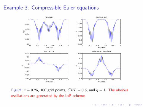
Example 3. Compressible Euler equations
0 0.2 0.4 0.6 0.8 10.9
0.92
0.94
0.96
0.98
1DENSITY
X−AXIS
rho
0 0.2 0.4 0.6 0.8 10.88
0.9
0.92
0.94
0.96
0.98
1PRESSURE
X−AXIS
p
0 0.2 0.4 0.6 0.8 1−0.2
−0.15
−0.1
−0.05
0
0.05
0.1
0.15VELOCITY
X−AXIS
v
0 0.2 0.4 0.6 0.8 12.4
2.45
2.5
2.55
2.6
2.65INTERNAL ENERGY
X−AXIS
e
Figure: t = 0.25, 100 grid points, CFL = 0.6, and q = 1. The obvious
oscillations are generated by the LxF scheme.

Example 3. Compressible Euler equations
0 0.2 0.4 0.6 0.8 10.93
0.94
0.95
0.96
0.97
0.98
0.99
1DENSITY
X−AXIS
rho
0 0.2 0.4 0.6 0.8 10.9
0.92
0.94
0.96
0.98
1PRESSURE
X−AXIS
p
0 0.2 0.4 0.6 0.8 1−0.1
−0.05
0
0.05
0.1VELOCITY
X−AXIS
v
0 0.2 0.4 0.6 0.8 12.4
2.45
2.5
2.55
2.6
2.65INTERNAL ENERGY
X−AXIS
e
Figure: Same as the last Figure except with q = 0.9. The solution is
non-oscillatory.

Example 3. Compressible Euler equations
0 0.2 0.4 0.6 0.8 10.95
0.96
0.97
0.98
0.99
1DENSITY
X−AXIS
rho
0 0.2 0.4 0.6 0.8 10.93
0.94
0.95
0.96
0.97
0.98
0.99
1PRESSURE
X−AXIS
p
0 0.2 0.4 0.6 0.8 1−0.06
−0.04
−0.02
0
0.02
0.04
0.06VELOCITY
X−AXIS
v
0 0.2 0.4 0.6 0.8 12.4
2.45
2.5
2.55
2.6INTERNAL ENERGY
X−AXIS
e
Figure: Same as before except that even points are used to discretize the
initial square-shaped signal. q = 1. No oscillation is present.

Local oscillations in the solutions by the GLF scheme
Remarks:
The presence of oscillations is not only related to the ways in
which the initial data are approximated, but also to the
numerical viscosity coefficient q.
For the LxF scheme, the local oscillations are very strong
although the TV property is not violated.
Those examples show that the different ways of initial
discretization lead to distinct solution behaviors. This
motivates the analysis of the discretization of initial data.
Outline
1 Motivation
2 Chequerboard modes in the initial discretization
3 Propagation of the chequerboard mode
4 Discrete Fourier analysis
5 Modified equation analysis
6 Conclusions

Chequerboard modes in the initial discretization
As observed previously and also in [M. Breuss, M2AN, 38(2004),
519-540], the numerical solutions display very distinct behaviors if
the initial data are discretized in different ways. This motivates us
to discuss the discretization of initial data
u(x, 0) = u0(x), x ∈ [0, 1], (2)
with M grid points and h = 1/M . For simplicity, we assume that
M is even, the initial function is periodic, i.e. u0(0) = u0(1) and
its value at the grid point xj is denoted by u0j . We express grid
function {u0j} by using the usual discrete Fourier sums with scaled
wave number ξ = 2πkh
u0j =
M/2∑k=−M/2+1
c0keiξj , i2 = −1, j = 0, 1, · · · ,M − 1, (3)

Chequerboard modes in the initial discretization
where the coefficients c0k are, in turn, expressed as
c0k =1
M
M−1∑j=0
u0je−iξj , k = −M/2 + 1, · · · ,M/2. (4)
We first pay special attention to the particular case that
c0k =
1, if k = M/2,
0, otherwise,
i.e. the initial data are taken to be just the highest Fourier mode
which is a single chequerboard mode
u0j = ei2πM2jh = eiπj = (−1)j .

Single square signal case.
We start with the simple initial data of a square signal such as
u0(x) =
1, 0 < x(1) < x < x(2) < 1,
0, otherwise,(5)
and take the following two ways to approximate the step function
(5) as a grid function: One uses an ODD number of grid points to
take the value one of the square signal and the other uses the next
smaller EVEN number of grid points. They could be seen as
approximations to some given fixed interval with end points not
represented on the mesh, which we do not explicitly specify here.

Single square signal case.
We use the discrete Fourier sum to clarify their difference.
(i) Discretization with an ODD number of grid points. Take
j1, j2 ∈ N such that j1 + j2 is an even number. We set
x(1) = (M2 − j1)h and x(2) = (M2 + j2)h. Discretize the square
signal (5) with p := j1 + j2 + 1 nodes, i.e. an odd number of grid
points, such that
u0j =
1, if j = M/2− j1, · · · ,M/2 + j2,
0, otherwise.(6)
Substituting them into (4), we obtain by simple calculation,
c0k = h
M−1∑j=0
u0je−iξj =
(−1)keiξj1 (1−e−iξp)
M(1−e−iξ) , for k 6= 0,
ph, for k = 0.(7)

Single square signal case.
Pay special attention to the term
c0M/2 = (−1)j1+M/2h,
since M is even and p is odd. Hence the initial data (6) can be
expressed in the form
u0j = (−1)j+j1+M/2h+ ph+∑
k 6=0,M/2
(−1)keiξ(j+j1)(1− e−iξp)M(1− e−iξ)
.
(8)
It turns out that chequerboard modes are present and will affect
the solutions if the initial data contains a square signal and are
discretized with an odd number of grid points.
Single square signal case.
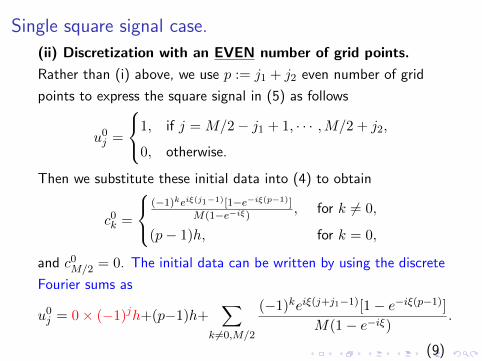
(ii) Discretization with an EVEN number of grid points.
Rather than (i) above, we use p := j1 + j2 even number of grid
points to express the square signal in (5) as follows
u0j =
1, if j = M/2− j1 + 1, · · · ,M/2 + j2,
0, otherwise.
Then we substitute these initial data into (4) to obtain
c0k =
(−1)keiξ(j1−1)[1−e−iξ(p−1)]
M(1−e−iξ) , for k 6= 0,
(p− 1)h, for k = 0,
and c0M/2 = 0. The initial data can be written by using the discrete
Fourier sums as
u0j = 0× (−1)jh+(p−1)h+∑
k 6=0,M/2
(−1)keiξ(j+j1−1)[1− e−iξ(p−1)]M(1− e−iξ)
.
(9)
Comparing (8) with (9), we observe an essential difference lies in
the fact that a checkerboard mode (−1)k+j1+M/2 is present in (8),
but it is filtered out in (9). This is closely related to the oscillatory
phenomenon observed in [M. Breuss, M2AN2004 & M2AN2005,
Tang & Warnecke, M2AN2004].

Step function initial data case
For more general piecewise constant initial data u0(x) there are
analogous discrete Fourier sum expressions. We divide the
computational domain [0, 1] into L subintervals
Il (l = 1, 2, · · · , L),⋃Ll=1 Il = [0, 1], the number of the discrete
points of a subinterval Il is Ml, M1 +M2 + · · ·+ML = M , and
the initial data (2) are expressed as
u0j =
L∑l=1
U l0 · χl(j), (10)
where U l0 are constants, χl(j) is the characteristic function on Il
χl(j) =
1, if xj ∈ Il,
0, otherwise .
Note that (10) can be regarded as the superposition of several
single square signals of the form (5).
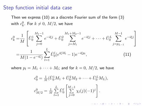
Step function initial data case
Then we express (10) as a discrete Fourier sum of the form (3)
with c0k. For k 6= 0, M/2, we have
c0k =1
M
U10
M1−1∑j=0
e−iξj + U20
M1+M2−1∑j=M1
e−iξj + · · ·+ UL0
M−1∑j=pL−1
e−iξj
=
1
M(1− e−iξ)
L∑l=1
U l0(eiξMl − 1)e−iξpl , (11)
where pl = M1 + · · ·+Ml; and for k = 0, M/2, we have
c00 = 1M (U1
0M1 + U20M2 + · · ·+ UL0 ML),
c0M/2 = 1M
L∑l=1
U l0
[M−1∑j=0
χl(j)(−1)j
].
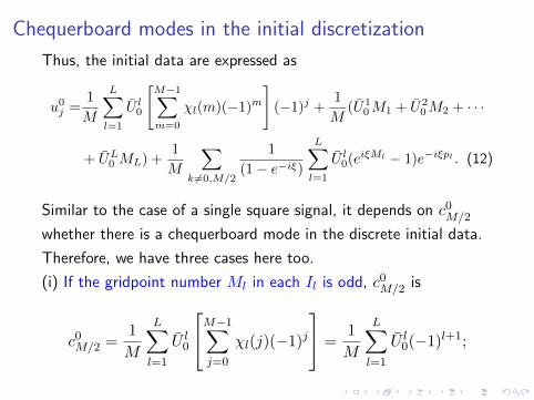
Chequerboard modes in the initial discretization
Thus, the initial data are expressed as
u0j =1
M
L∑l=1
U l0
[M−1∑m=0
χl(m)(−1)m
](−1)j +
1
M(U1
0M1 + U20M2 + · · ·
+ UL0 ML) +1
M
∑k 6=0,M/2
1
(1− e−iξ)
L∑l=1
U l0(eiξMl − 1)e−iξpl . (12)
Similar to the case of a single square signal, it depends on c0M/2
whether there is a chequerboard mode in the discrete initial data.
Therefore, we have three cases here too.
(i) If the gridpoint number Ml in each Il is odd, c0M/2 is
c0M/2 =1
M
L∑l=1
U l0
M−1∑j=0
χl(j)(−1)j
=1
M
L∑l=1
U l0(−1)l+1;
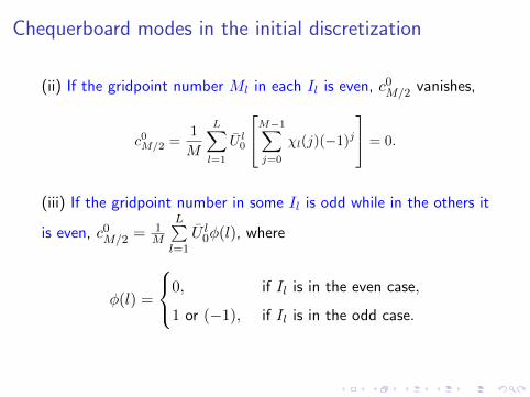
Chequerboard modes in the initial discretization
(ii) If the gridpoint number Ml in each Il is even, c0M/2 vanishes,
c0M/2 =1
M
L∑l=1
U l0
M−1∑j=0
χl(j)(−1)j
= 0.
(iii) If the gridpoint number in some Il is odd while in the others it
is even, c0M/2 = 1M
L∑l=1
U l0φ(l), where
φ(l) =
0, if Il is in the even case,
1 or (−1), if Il is in the odd case.

Chequerboard modes in the initial discretization
Thus, there is no chequerboard mode for Case (ii). For Case (i),
the summation may be zero when the factors cancel. However,
since this summation is taken in the global sense and the
chequerboard mode exists in each subinterval, the solution may
still contain oscillations due to the finite propagation speed
property of the scheme.

Chequerboard modes in the initial discretization
We summarize all of the above analysis as follows.
Proposition
Suppose that the initial data
u(x, 0) = u0(x)
are given as a step function. We can approximate them as the
superposition of several single square signals. For each square
signal we have two different types of discretizations. If they are
approximated with an ODD number of grid points, the
chequerboard (i.e. highest frequency) mode is present. In contrast,
if they are discretized with an EVEN number of grid points, there
is no chequerboard mode.

Outline
1 Motivation
2 Chequerboard modes in the initial discretization
3 Propagation of the chequerboard mode
4 Discrete Fourier analysis
5 Modified equation analysis
6 Conclusions
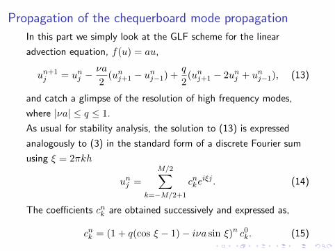
Propagation of the chequerboard mode propagation
In this part we simply look at the GLF scheme for the linear
advection equation, f(u) = au,
un+1j = unj −
νa
2(unj+1 − unj−1) +
q
2(unj+1 − 2unj + unj−1), (13)
and catch a glimpse of the resolution of high frequency modes,
where |νa| ≤ q ≤ 1.
As usual for stability analysis, the solution to (13) is expressed
analogously to (3) in the standard form of a discrete Fourier sum
using ξ = 2πkh
unj =
M/2∑k=−M/2+1
cnkeiξj . (14)
The coefficients cnk are obtained successively and expressed as,
cnk = (1 + q(cos ξ − 1)− iνa sin ξ)n c0k. (15)

Corresponding to the two kinds of discretization of a single square
signal, c0j have different expressions, and the solutions become:
(i) Odd discretization case. With the initial data (8), the
solution of (13) is
unj =1
M(1− 2q)n(−1)j+j1+M/2 +
M/2−1∑k=−M/2+1
cnkeiξj . (16)
(ii) Even discretization case. With the initial data (9), we have
unj = 0× (1− 2q)n(−1)j +
M/2−1∑k=−M/2+1
cnkeiξj . (17)
Comparing them, we see that in the odd case the chequerboard
mode does not vanish if it exists initially, unless we have the MLF
scheme q = 1/2, although it decays with a rate of |2q − 1| at each
time step. So, a proper discretization of initial data would be
important to avoid these possible oscillations in solving CL.

0 0.2 0.4 0.6 0.8 10
0.1
0.2
0.3
0.4
0.5
0.6
0.7
u
(a) q=1.00 0.2 0.4 0.6 0.8 1
0
0.1
0.2
0.3
0.4
0.5
0.6
0.7
u
(b) q=0.85
0 0.2 0.4 0.6 0.8 10
0.1
0.2
0.3
0.4
0.5
u
(c) q=0.750 0.2 0.4 0.6 0.8 1
0
0.1
0.2
0.3
0.4
0.5
u(d) q=0.5
Figure: The decay of oscillations as the parameter q decreases: The
initial data are impulse signal, the CFL number is 0.2 and only one time
step is taken.
Remark 1. The solution of LxF unj = (−1)n+j oscillates between 1
and −1 alternately if the chequerboard mode initial data are taken.
The large numerical dissipation does not have any effect.
Remark 2. In case 0 < q < 1, the chequerboard mode is damped
out quickly. In particular, for the MLF q = 1/2 the chequerboard
mode is eliminated and has no influence on the solution at all.
In the following we attempt to analyze the numerical dissipation
and phase error mechanisms of GLF, particularly on high frequency
modes and explain the phenomenon of oscillations caused by high
frequency modes. We apply discrete Fourier analysis and the
method of modified equation analysis. Both of the methods give
complimentary results, which are consistent. We show that as
0 ≤ q ≤ 1 is away from 1/2, the damping on high frequency modes
becomes weak. In particular, there is no damping effect in the LxF
scheme (i.e. q = 1) and the unstable central scheme (i.e. q = 0).

Outline
1 Motivation
2 Chequerboard modes in the initial discretization
3 Propagation of the chequerboard mode
4 Discrete Fourier analysis
5 Modified equation analysis
6 Conclusions
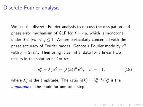
Discrete Fourier analysis
We use the discrete Fourier analysis to discuss the dissipation and
phase error mechanism of GLF for f = au, which is monotone
under 0 < |νa| < q ≤ 1. We are particularly concerned with the
phase accuracy of Fourier modes. Denote a Fourier mode by eiξ
with ξ = 2πkh. Then using it as initial data for a linear FDS
results in the solution at t = nτ
unk = λnkeiξ = (λ(k))n eiξ, i2 = −1, (18)
where λnk is the amplitude. The ratio λ(k) = λn+1k /λnk is the
amplitude of the mode for one time step.
Discrete Fourier analysis
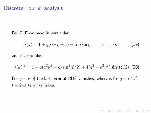
For GLF we have in particular
λ(k) = 1 + q(cos ξ − 1)− iνa sin ξ, ν = τ/h, (19)
and its modulus
|λ(k)|2 = 1 + 4(a2ν2 − q) sin2(ξ/2) + 4(q2 − a2ν2) sin4(ξ/2). (20)
For q = ν|a| the last term at RHS vanishes, whereas for q = ν2a2
the 2nd term vanishes.

Discrete Fourier analysisAlso we see that for GLF, under the conditions 0 < ν2a2 ≤ q ≤ 1,
we have from (20) the estimate of the modulus of amplitude
|λ(k)|2 = 1+4(a2ν2−q)(sin2(ξ/2)− sin4(ξ/2)
)+4q(q−1) sin4(ξ/2) ≤ 1.
(21)
Thus these conditions imply that the schemes are linearly stable.
In fact, these conditions are necessary and sufficient for stability.
Figure: Range of stability of parameter q over CFL number νa.

Discrete Fourier analysis
The exact solution of the Fourier mode eiξ for x = h after one
time step τ is ei(ξ−2πakτ) = e−i2πakτeiξ = λexact(k)eiξ. The exact
amplitude λexact(k) has modulus 1. We see from (20) that the
amplification error, i.e. the error in amplitude modulus, is of order
O(ξ) for the monotone schemes and order O(ξ2) for the LW
scheme. If the modulus of λ(k) is less than one, the effect of the
multiplication of a solution component with λ(k) is called
numerical dissipation and then the amplification error is called
dissipation error. If the modulus is larger than 1, this leads to the
amplification of the Fourier mode, i.e. instability of any solution
containing it. Further, comparing the exponents of λ(k) and
λexact(k) there is a phase error arg λ(k)− (−2πakτ).
Discrete Fourier analysis
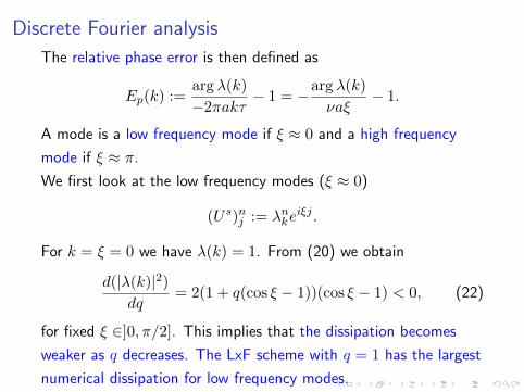
The relative phase error is then defined as
Ep(k) :=arg λ(k)
−2πakτ− 1 = −arg λ(k)
νaξ− 1.
A mode is a low frequency mode if ξ ≈ 0 and a high frequency
mode if ξ ≈ π.
We first look at the low frequency modes (ξ ≈ 0)
(U s)nj := λnkeiξj .
For k = ξ = 0 we have λ(k) = 1. From (20) we obtain
d(|λ(k)|2)dq
= 2(1 + q(cos ξ − 1))(cos ξ − 1) < 0, (22)
for fixed ξ ∈]0, π/2]. This implies that the dissipation becomes
weaker as q decreases. The LxF scheme with q = 1 has the largest
numerical dissipation for low frequency modes.

Discrete Fourier analysis
The phase of the low frequency modes is approximated by Taylor
expansion at ξ = 0
arg λ = arctan
(−νa sin ξ
1 + q[cos ξ − 1]
)≈ −νaξ
(1 +
3q − 1− 2ν2a2
6ξ2 + · · ·
).
This phase has a relative error Ep(k) of order O(ξ2). For the LW
scheme, this phase error causes oscillations, which cannot be
suppressed by the weaker dissipation of order O(ξ2), compared to
the dissipation error O(ξ) of the upwind scheme.

Discrete Fourier analysis
For high frequency modes (18), ξ ≈ π, the situation is very
different. We introduce the decomposition ξ = π + ξ′, i.e.
ξ′ = 2πk′h with kh = 1/2 + k′h, and thus ξ′ ≈ 0. We write the
modes in the form
(Uh)nj = λnkeiξj = λnke
i(π+ξ′)j = (−1)j+nλnk′eiξ′j , (23)
with λnk′ = (−1)j+neiπjλnk and set
(Uo)nj := λnk′eiξ′j .
The factor (Uo)nj can be regarded as a perturbation amplitude of
the chequerboard modes (eiπ)j+n = (−1)j+n. The dissipation
(amplitude error) depends only on λnk′ . Then substituting (Uh)njinto (13) yields
λ′ := λn+1k′ /λnk′ = −1 + q(1 + cos ξ′)− iνa sin ξ′.

Therefore, we have
|λ′|2 =(1− q(1 + cos ξ′))2 + ν2a2 sin2 ξ′
=1 + 4(a2ν2 − q) cos2(ξ′/2) + 4(q2 − a2ν2) cos4(ξ′/2). (24)
It is consistent with a shift of π in the variable ξ in (20).
Regarding the high frequency modes, for all schemes the amplitude
error is O(1). At ξ′ = 0 we have
|λ′|2 = 1− 4q(1− q), (25)
so we have the lowest amplitude error for q = 1 or near zero, the
highest for the modified LxF scheme with q = 1/2. Obviously, for
small ξ′, |λ′|2 is an increasing function of q if q > 1/2 because
d(|λ′|2)/dq = −2[1− q(1 + cos(ξ′))](1 + cos ξ′) > 0. (26)
That is, GLF becomes much more dissipative for high frequency
modes as the parameter q decreases, which is in sharp contrast
with the situation for low frequency modes, see (22).

Furthermore, let us look at the relative phase error. We compute
arg λ′ = tan−1(
−νa sin ξ′
−1 + q(1 + cos ξ′)
)=−νaξ′
2q − 1− νa
3(2q − 1)2
[q + 1
2− ν2a2
2q − 1
]ξ′3 +O(ξ′5). (27)
Then for the high frequency modes (Uh)nj , we have by recalling
that ξ = π + ξ′
(Uh)nj =(−1)j+nλ′nk eiξ′j
=|λ′|nei(jξ−2πkanτ) · ein(−π+arg λ′+νaξ).
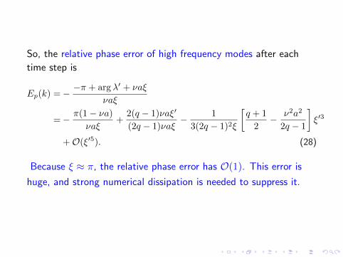
So, the relative phase error of high frequency modes after each
time step is
Ep(k) =− −π + arg λ′ + νaξ
νaξ
=− π(1− νa)
νaξ+
2(q − 1)νaξ′
(2q − 1)νaξ− 1
3(2q − 1)2ξ
[q + 1
2− ν2a2
2q − 1
]ξ′3
+O(ξ′5). (28)
Because ξ ≈ π, the relative phase error has O(1). This error is
huge, and strong numerical dissipation is needed to suppress it.

We summarize the above Fourier analysis in the proposition.
Proposition
We distinguish low and high frequency Fourier modes unj = λnkeijξ,
ξ = 2πkh, and they behave differently.
(i) For the low frequency modes (ξ ∼ 0), the relative phase error is
of order O(ξ2), and the amplitude error (dissipation) becomes
smaller as the parameter q decreases. The order of amplitude error
is O(ξ) for the monotone schemes and O(ξ2) for the LW scheme.
(ii) For the high frequency modes (ξ ∼ π), the relative phase error
is of order O(1), the amplitude error becomes larger as the
parameter q is closer to 1/2.

Outline
1 Motivation
2 Chequerboard modes in the initial discretization
3 Propagation of the chequerboard mode
4 Discrete Fourier analysis
5 Modified equation analysis
6 Conclusions

Modified equation analysis for linear cases
As we know, the amplitude error and relative phase error of the
Fourier modes have a correspondence with dissipation and phase
error mechanisms displayed by related PDEs. Here we use the
modified equation to further investigate the mechanisms of
dissipation and phase error of GLF. Particularly, we want to see
how the dissipation offsets the large phase error of high frequency
modes. The modified equation analysis was originally introduced
for low frequency modes1. Here it is especially used for high
frequency modes, as its usefulness was clearly shown in [K.W.
Morton and D.F. Mayers, Numerical Solution of Partial Differential
Equations, Cambridge Univ Press, 2005].
The modified equation is derived by first expanding each term of a
difference scheme in a Taylor series and then eliminating time
derivatives higher than first order by certain algebraic
manipulations.1R. F. Warming and B. J. Hyett, The modified equation approach to the
stability and accuracy analysis of finite-difference methods, J. Comput. Phys.,
14(1974), 159-179

Modified equation analysis for linear cases
We begin here with the linear case, and still use notation ν = τ/h.
As in [Morton & Mayers, 2005, P173], we will consider a smooth
solution (U s)nj and an oscillatory solution (Uh)nj , respectively. The
oscillatory solution (Uh)nj is written as
(Uh)nj = (−1)j+n(Uo)nj , (29)
where (Uo)nj is viewed as the perturbation amplitude of the
chequerboard mode.

Modified equation analysis for linear cases
The smooth solution (U s)nj satisfies GLF, i.e.
(Us)n+1j = (Us)nj−
νa
2((Us)nj+1−(Us)nj−1)+
q
2((Us)nj+1−2(Us)nj +(Us)nj−1).
Then we derive a modified equation for this solution2, and the
notation U s corresponds to the associated exact solution
∂tUs+a∂xU
s =1
2τ
(qh2 − a2τ2
)∂2xU
s+a
(−h
2
6+
1
2qh2 − 1
3a2τ2
)∂3xU
s+· · · .
It is evident that the numerical viscosity of GLF becomes stronger
for low frequency modes as q is larger, and vice versa. Particularly,
for the LW scheme the dissipation comes from the 4th order term
and therefore is quite weak. This is consistent with the fact
observed by the Fourier analysis that the dissipation becomes
weaker as q decreases, provided that the scheme is stable.2K.W. Morton & D.F. Mayers, CUP, 2005, p169
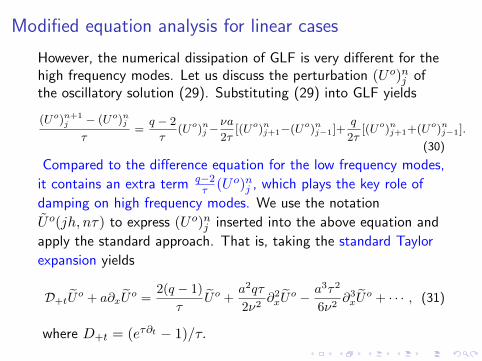
Modified equation analysis for linear cases
However, the numerical dissipation of GLF is very different for thehigh frequency modes. Let us discuss the perturbation (Uo)nj ofthe oscillatory solution (29). Substituting (29) into GLF yields
(Uo)n+1j − (Uo)nj
τ=q − 2
τ(Uo)nj−
νa
2τ[(Uo)nj+1−(Uo)nj−1]+
q
2τ[(Uo)nj+1+(Uo)nj−1].
(30)
Compared to the difference equation for the low frequency modes,
it contains an extra term q−2τ (Uo)nj , which plays the key role of
damping on high frequency modes. We use the notation
Uo(jh, nτ) to express (Uo)nj inserted into the above equation and
apply the standard approach. That is, taking the standard Taylor
expansion yields
D+tUo + a∂xU
o =2(q − 1)
τUo +
a2qτ
2ν2∂2xU
o − a3τ2
6ν2∂3xU
o + · · · , (31)
where D+t = (eτ∂t − 1)/τ.

Note that in (30) the term q−2τ (Uo)nj is unusual compared to
classical modified equation analysis.
We may derive the modified equation for the oscillatory part
∂tUo+
a
2q − 1∂xU
o =ln |2q − 1|
τUo +
h2
2τ
[q(2q − 1)− ν2a2]
(2q − 1)2∂2xU
o
+ah2
6
[(q + 1)(2q − 1)− 2ν2a2]
(2q − 1)3∂3xU
o + · · · .
Introducing for q 6= 1/2 a rescaling x′ = x(2q − 1) and omitting
the use of a primed variable gives
∂tUo+a∂xU
o =ln |2q − 1|
τUo +
h2
2τ[q(2q − 1)− ν2a2]∂2xUo
+ah2
6[(q + 1)(2q − 1)− 2ν2a2]∂3xU
o + · · · .
Unlike the modified equation (52) for the low frequency modes the
numerical dissipation comes from two terms: Zero order termln |2q−1|
τ Uo and the 2nd order term a2τ2ν2a2
[q(2q − 1)− ν2a2]∂2xUo.The former exerts more dominant dissipation than the latter.
Modified equation analysis for linear cases
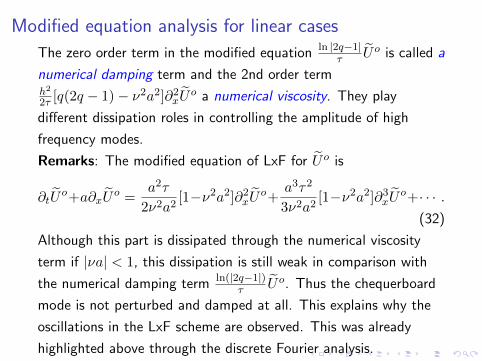
The zero order term in the modified equation ln |2q−1|τ Uo is called a
numerical damping term and the 2nd order termh2
2τ [q(2q − 1)− ν2a2]∂2xUo a numerical viscosity. They play
different dissipation roles in controlling the amplitude of high
frequency modes.
Remarks: The modified equation of LxF for Uo is
∂tUo+a∂xU
o =a2τ
2ν2a2[1−ν2a2]∂2xUo+
a3τ2
3ν2a2[1−ν2a2]∂3xUo+· · · .
(32)
Although this part is dissipated through the numerical viscosity
term if |νa| < 1, this dissipation is still weak in comparison with
the numerical damping term ln(|2q−1|)τ Uo. Thus the chequerboard
mode is not perturbed and damped at all. This explains why the
oscillations in the LxF scheme are observed. This was already
highlighted above through the discrete Fourier analysis.
Modified equation analysis for linear cases
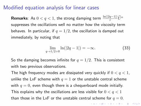
Remarks: As 0 < q < 1, the strong damping term ln(|2q−1|)τ Uo
suppresses the oscillations well no matter how the viscosity term
behaves. In particular, if q = 1/2, the oscillation is damped out
immediately, by noting that
limq→1/2+0
ln(|2q − 1|) = −∞. (33)
So the damping becomes infinite for q = 1/2. This is consistent
with two previous observations.
The high frequency modes are dissipated very quickly if 0 < q < 1,
unlike the LxF scheme with q = 1 or the unstable central scheme
with q = 0, even though there is a chequerboard mode initially.
This explains why the oscillations are less visible for 0 < q < 1
than those in the LxF or the unstable central scheme for q = 0.
Outline
1 Motivation
2 Chequerboard modes in the initial discretization
3 Propagation of the chequerboard mode
4 Discrete Fourier analysis
5 Modified equation analysis
6 Conclusions

Conclusions
The talk discussed the local oscillations in the GLF scheme. It
has general implications into more extensive (monotone)
schemes and multidimensional cases.
The discrete Fourier analysis and the modified equation are
applied to investigating the numerical dissipative and
dispersive mechanisms as well as relative phase errors.
The resolutions of the low and high frequency modes
unj = λnkeijξ, ξ = 2πkh in numerical solutions are individually
discussed.
The presence of high frequency modes results from the
initial/boundary conditions. The discretization may produce
the chequerboard modes.
Conclusions
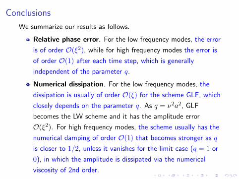
We summarize our results as follows.
Relative phase error. For the low frequency modes, the error
is of order O(ξ2), while for high frequency modes the error is
of order O(1) after each time step, which is generally
independent of the parameter q.
Numerical dissipation. For the low frequency modes, the
dissipation is usually of order O(ξ) for the scheme GLF, which
closely depends on the parameter q. As q = ν2a2, GLF
becomes the LW scheme and it has the amplitude error
O(ξ2). For high frequency modes, the scheme usually has the
numerical damping of order O(1) that becomes stronger as q
is closer to 1/2, unless it vanishes for the limit case (q = 1 or
0), in which the amplitude is dissipated via the numerical
viscosity of 2nd order.
Conclusions
In the LW scheme the oscillations are caused by the relative
phase error of low frequency modes, while in LxF, oscillations
are caused by the relative phase error of high frequency
modes. To control the oscillations by high frequency modes,
the strong numerical damping is necessary to add.
Compared to LxF, the GLF (0 < q < 1) introduces the
numerical damping as well, which is stronger as q is closer to
1/2. Hence, to control the oscillations caused by high
frequency modes, the numerical damping plays an important
role.

Conclusions
Indeed, the GLF scheme is monotone and thus TVD under a
certain restriction. The TVD property is proposed to describe
the global property of solutions of CLs. The oscillations we
are investigating is local and does not contradict to this global
TVD property. As far as hyperbolic problems are concerned,
local properties should be paid more attention because of
finite propagation of waves.

Thank you for your attention!
J.Q. Li, H.Z. Tang, G. Warnecke,& L.M. Zhang, Math. Comp.,
78(2009), 1997-2018.