local one class optimization gal chechik, stanford joint work with koby crammer, hebrew university...
Post on 20-Dec-2015
220 views
TRANSCRIPT
Local one class optimization
Gal Chechik, Stanford
joint work with Koby Crammer, Hebrew university of Jerusalem

The one-class problem:
Find a subset of similar/typical samplesFormally: find a ball of a given radius (with some metric) that covers as many data points as possible (related to the set covering problem).

Motivation I
Unsupervised setting: Sometimes we wish to model small parts of the data and ignore the rest. This happens when many data points are irrelevant.
Example: – Finding sets of co-expressed
genes in genome wide-experiment: identify the relevant genes out of thousands irrelevant ones.
– Finding a set of document of the same topic, in an heterogeneous corpus

Motivation II
Supervised setting: Learning given positive samples only
Examples: – Protein interactions– Intrusion detection application
Care about low false positive rate

Current approaches
Often treat the problem as Outliers and novelty detection:
most samples are relevantCurrent approaches use
– A convex cost function (Schölkopf 95, Tax and Duin 99, Ben-Hur et al 2001).
– A parameter that affects the size or weight of the ball
• Bias towards center of mass
When searching for a small ball, the center of the optimal ball is in the global center of mass, w*=argmin Σx(x-w)2 missing the
interesting structures.

Example with synthetic data:– 2 Gaussians + uniform background
Convex one class (OSU-SVM)
Local one-class
Current approaches

How do we do it:
1. A cost function designed for small sets2. A probabilistic approach: allow soft
assignment to the set3. Regularized optimization

1. A cost function for small sets
• The case where only few samples are relevant
• Use cost function that is flat for samples not in the set
– Two parameters:• Divergence measure DBF
• Flat cost K
– Indifferent to the position of “irrelevant” samples.
– Solutions converge to the center of mass when ball is large.

2. A probabilistic formulation
• We are given m samples in a d dimensional space or simplex, indexed by x .
• p(x) is the prior distribution over samples• c ={TRUE,FALSE} is an R.V. that characterizes
assignment to the interesting set (the “Ball”).• p(c|x) reflects our belief that the sample x is
“interesting”.• The cost function will be
D=p(c|x)DBF(w|vx) + (1-p(c|x))KDBF is a divergence measure, to be discussed later
m mx x 1{ } v

3. Regularized optimization
The goal: minimize the mean cost+regularization
min β <DBF,K(,wC;vx)>p(c,x) + I(C;X) {p(c|x),w}
• The first term: measures the mean distortion<DBF,R(p(c|x),w;vx)> = Σ p(x) [p(c|x)BF(w|vx)+(1-p(c|x))K]
• The second term: regularizes the compression of the data (removes information about X)
I(C;X) = H(X) – H(X|C),
It pushes for putting many points in the set.• This target function is not convex

To solve the problem
• It turns out that for a family of divergence functions, called Bregman divergences, we can analytically describe properties of the optimal solution.
• The proof follows the analysis of the Information Bottleneck method (Tishby,Pereira,Bialek,99)

Bregman divergences
• A Bregman divergence is defined by a convex function F (in our case F(v)=Σf(vi))
• Common examples: L2 norm f(x)=½x2
Itkura-Saito f(x)=-log(x)DKL f(x)=xlog(x)
Unnormalized relative entropy f(x)=xlogx-x
• Lemma: Convexity of the Bregman BallThe set of points {v s.t. BF(v||w)<R} is convex
FB (v||w) F(v) [F(w) F(w)(v w)]

Properties of the solution
OC solutions obey three fixed point equations
When β→∞,
Best assignment for x is to minimize
x
1p(x)p(c|x)
p(c) w v
F x
1 p(c)p(c|x) 1/ 1 exp [B (v ||w) K]
p(c)
p(c) p(c|x)p(x)
F x
F x
F x
1 B ( || ) K
limp(c|x) 0 B ( || ) K
p(c) B ( || ) K
v w
v w
v w
F xLoss min(B (v ||w),K)

The effect of the K
• K controls the nature of the solution. – Is the cost of leaving a point out of the ball – Large K => large radius & many points in set
– For the L2 norm, K is formally related to the prior of a single Gaussian fit to the subset.
• A full description of a data may require to solve for the complete spectrum of K values.

Algorithm: One-Class IB
Adapting the sequential-IB algorithm: One-Class IB:Input: set of m points vx, divergence BF, cost K
Output: centroid w, assignment p(c|x)Optimization method:
– Iteratively operating sample-by-sample, try to modify the status of a single sample
– One step Look-ahead re-fit the model and decide if to change assignment of a sample
– This uses a simple formula because of the nice properties of Bregman divergences
– search in the dual space of samples, rather than parameters w.

Experiments 1: information retrievalFive most frequent categories of
Reuters21578.Each document represented as a multinomial
distribution over 2000 terms.The experimental setup: For each category:
– train with half of the positive documents, – test with all rest of documents
Compared one-class IB with One-class Convex which uses a convex loss function (Crammer&
Singer-2003). Controlled by a single parameter η, that determines weight of the class.

Experiments 1: information retrievalCompare precision recall performance, for a
range or K/μ values.
recall
prec
isio
n

Experiments 1: information retrievalCentroids of clusters, and their distances
from the center of mass

Experiments 2: gene expression
A typical application for searching small but interesting sets of genes.
Genes represented by expression profile across tissues from different patientsAlizadeh-2000, (B-cell lymphoma tissues) has mortality data which can be used as an objective method for validating quality of the genes selected.
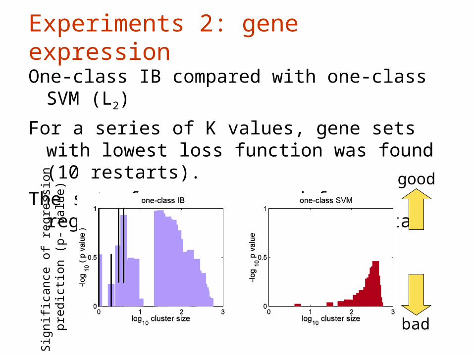
Experiments 2: gene expression
One-class IB compared with one-class SVM (L2)
For a series of K values, gene sets with lowest loss function was found (10 restarts).
The set of genes was used for regression vs, the mortality data.
Sig
nific
ance
of
regr
essi
on
pred
ictio
n (p
- va
lue)
good
bad
Future work: finding ALL relevant subsets• Complete characterization of all interesting
subsets in the data. • Assume we have a function that assign an
interest value to each subset. We search in the space of subsets and for all local maxima.
• Requires to define the locality. A natural measure of locality in the subsets-space is the Hamming distance.
• The complete characterization of the data require description using a range of local neighborhoods.

Future work: multiple one-class
• Synthetic example: two overlapping Gaussians and background uniform noise

Conclusions
• We focus on learning one-class for cases where a small ball is sought.
• Formalize the problem using IB, and derive its formal solutions
• One-class IB performs well in the regime of small subsets.