local governments and economic freedom - mercatus … · local governments and economic freedom ......

Local Governments and Economic Freedom

A Test of the Leviathan Hypothesis

Adam A. Millsap, Bradley K. Hobbs, and Dean Stansel

MERCATUS WORKING PAPER

All studies in the Mercatus Working Paper series have followed a rigorous process of academic evaluation, including (except where otherwise noted) at least one double-blind peer review. Working Papers present an author’s provisional findings, which, upon further consideration and revision, are likely to be republished in an academic journal. The opinions expressed in Mercatus Working Papers are the authors’ and do not represent

official positions of the Mercatus Center or George Mason University.

Adam A. Millsap, Bradley K. Hobbs, and Dean Stansel. “Local Governments and Economic Freedom: A Test of the Leviathan Hypothesis.” Mercatus Working Paper, Mercatus Center at George Mason University, Arlington, VA, 2017. Abstract Geoffrey Brennan and James M. Buchanan, in their 1980 book The Power to Tax, hypothesize that “the potential for fiscal exploitation varies inversely with the number of competing governmental units in the inclusive territory.” This paper tests that theory at the local level using data for US metropolitan statistical areas (MSA). MSAs are constructed on the basis of commuting patterns and are meant to delineate the local economy. Because of their construction, MSAs typically contain several distinct and nonoverlapping political jurisdictions, each with the power to tax residents, mitigate local externalities, and provide local public goods. Following previous literature, we measure “competing governmental units” using the number of general-purpose local governments within an MSA, adjusted for land area and population. In contrast to previous work, which uses less comprehensive measures of “fiscal exploitation,” we test Brennan and Buchanan’s “Leviathan hypothesis” using various measures of MSA economic freedom, rather than more limited measures of spending or revenue, as our dependent variable. We find mixed evidence that the number of competing jurisdictions is positively associated with economic freedom. When examining the individual components of economic freedom, we find a positive and statistically significant relationship with labor market freedom but only a weak relationship with government spending or taxes. These results offer mixed support for the Leviathan hypothesis, though support strengthens when metro areas in the South are excluded. JEL codes: H77, H71, R23 Keywords: federalism, local taxation, decentralization, regional migration, economic freedom Author Affiliation and Contact Information Adam A. Millsap Bradley K. Hobbs Dean Stansel Florida State University Clemson University Southern Methodist University [email protected] [email protected] [email protected] Copyright 2017 by Adam A. Millsap, Bradley K. Hobbs, Dean Stansel, and the Mercatus Center at George Mason University This paper can be accessed at https://www.mercatus.org/publications/local-governments -economic-freedom-leviathan

https://www.mercatus.org/publications/local-governments-economic-freedom-leviathan

https://www.mercatus.org/publications/local-governments-economic-freedom-leviathan

3

Local Governments and Economic Freedom: A Test of the Leviathan Hypothesis

Adam A. Millsap, Bradley K. Hobbs,* and Dean Stansel

1. Introduction

In their 1980 book The Power to Tax, Geoffrey Brennan and James M. Buchanan propose the so-

called Leviathan hypothesis: “The potential for fiscal exploitation varies inversely with the

number of competing governmental units in the inclusive territory.”1 Although governments

often hold substantial power over their particular political entities, they are limited by

competition from proximate governments in their power to extract monopoly rents. Here, we

investigate the Leviathan hypothesis in the framework of competing local governments.

Competition among nearby political entities limits the monopoly power of each entity, thus

making local economies more dynamic and robust. The ability of competition to restrict

Leviathan is particularly important to the success of small business entrepreneurs. (This idea is

related to Weingast’s concept of “market-preserving federalism.”2)

The Leviathan hypothesis posits that horizontal competition occurs among

governmental entities when the tax base is mobile and has choice. Firms and entrepreneurs

use the leverage of exit to maximize their preferred array of services, amenities, and tax

treatment across alternatives in a form of “horizontal” competition. The Leviathan model has

been subjected to numerous empirical tests. Most of that literature relies on levels of taxation

or spending as the measure of what Brennan and Buchanan referred to as “fiscal exploitation.”

Thus, the focus has been on the ability of governments to tax and spend and on the effects of

* Dr. Hobbs is the contact author for this paper. 1 Geoffrey Brennan and James M. Buchanan, The Power to Tax (New York: Cambridge University Press,1980), 211. 2 Barry Weingast, “The Economic Role of Political Institutions: Market-Preserving Federalism and Economic Development,” Journal of Law, Economics and Organization 11, no. 1 (1995): 1–31.

4

this ability on two things: the financial viability of a political entity—be it a nation, state, or

municipality—and the response of citizens to it. This empirical literature is mixed, though

subnational studies have been more likely to confirm the Leviathan hypothesis.3 For example,

Richard E. Wagner and Warren E. Weber;4 David L. Sjoquist;5 Thomas J. DiLorenzo;6 Mark

Schneider;7 Michael A. Nelson;8 Jeffrey Zax;9 Randall W. Eberts and Timothy J. Gronberg;10

David Joulfaian and Michael L. Marlow;11 Dean Stansel;12 Michael Craw;13 Joshua Hall and

Justin Ross;14 Lars P. Feld, Gebhard Kirchgassner, and Christoph A. Schaltegger;15 and

3 Ryan Yeung, “The Effects of Fiscal Decentralization on the Size of Government: A Meta-Analysis,” Public Budgeting and Finance 29, no. 4 (2009): 1–23. Confirmatory results at the national level include Thushyanthan Baskaran, “On the Link between Fiscal Decentralization and Public Debt in OECD Countries,” Public Choice 145 (2010): 351–78; and Jason Sorens, “The Institutions of Fiscal Federalism,” Publius 41, no. 2 (2011): 207–31. 4 Richard E. Wagner and Warren E. Weber, “Competition, Monopoly, and the Organization of Government in Metropolitan Areas,” Journal of Law and Economics 18, no. 3 (1975): 670–84. 5 David L. Sjoquist, “The Effect of the Number of Local Governments on Central City Expenditures,” National Tax Journal 35, no. 1 (1982): 79–87. 6 Thomas J. DiLorenzo, “Economic Competition and Political Competition: An Empirical Note,” Public Choice 40, no. 2 (1983): 203–9. 7 Mark Schneider, “Fragmentation and the Growth of Local Government,” Public Choice 48, no. 3 (1986): 255–64; Mark Schneider, The Competitive City: The Political Economy of Suburbia (Pittsburgh, PA: University of Pittsburgh Press, 1989); Mark Schneider, “Intercity Competition and the Size of the Local Public Work Force,” Public Choice 63, no. 3 (1989): 253–65. 8 Michael A. Nelson, “An Empirical Analysis of State and Local Tax Structure in the Context of the Leviathan Model of Government,” Public Choice 49, no. 3 (1986): 283–94; Michael A. Nelson, “Searching for Leviathan: Comment and Extension,” American Economic Review 77, no. 1 (1987): 198–204. 9 Jeffrey Zax, “Is There a Leviathan in Your Neighborhood?,” American Economic Review 79, no. 3 (1989): 560–67. 10 Randall W. Eberts and Timothy J. Gronberg, “Structure, Conduct, and Performance in the Local Public Sector,” National Tax Journal 43, no. 2 (1990): 165–73. 11 David Joulfaian and Michael L. Marlow, “Government Size and Decentralization: Evidence from Disaggregated Data,” Southern Economic Journal 56, no. 4 (1990): 1094–1102. 12 Dean Stansel, “Interjurisdictional Competition and Local Government Spending in U.S. Metropolitan Areas,” Public Finance Review 34, no. 2 (March 2006): 173–94. 13 Michael Craw, “Taming the Local Leviathan: Institutional and Economic Constraints on Municipal Budgets,” Urban Affairs Review 43, no. 5 (2008): 663–90. 14 Joshua Hall and Justin Ross, “Tiebout Competition, Yardstick Competition, and Tax Instrument Choice: Evidence from Ohio School Districts,” Public Finance Review 38, no. 6 (2010): 710–37. 15 Lars P. Feld, Gebhard Kirchgassner, and Christoph A. Schaltegger, “Decentralized Taxation and the Size of Government: Evidence from Swiss State and Local Governments,” Southern Economic Journal 77, no. 1 (2010): 27–48.

5

George R. Crowley and Russell S. Sobel16 all found subnational evidence to support the

Leviathan hypothesis.17

Notable exceptions that contradict the model are Wallace E. Oates,18 Kevin F. Forbes and

Ernest Zampelli,19 Campbell and Mitchell,20 and Alfred M. Wu and Mi Lin.21 Campbell and

Mitchell also reject the Leviathan model. They argue that economic freedom at the state level

converges over time and place as political party majorities consolidate power. They contend that

majorities matter because they reduce the “logrolling and monitoring costs” associated with the

agreements made quid pro quo to entice political opponents to support legislation that they

initially reject. The net effect is that the size of government falls as political majorities

consolidate—or, as Campbell and Mitchell put it, “What we fail to find . . . is evidence that both

parties would prefer a larger, more expansive government than the one preferred by the median

voter.”22 So, the response of poltiticians to strong median voter preference may lead to the

observed conflicting empirical results with the Leviathan model. Wu and Lin find that “fiscal

decentralization in China does not curb bureaucratic expansion. Rather, the revenue sharing

16 George R. Crowley and Russell S. Sobel, “Does Fiscal Decentralization Constrain Leviathan? Evidence from Local Property Tax Competition,” Public Choice 149, no. 1–2 (2011): 5–30. 17 In what was not explicitly a test of the Leviathan hypothesis, Gaines H. Liner examined cities in 43 states and found that more lenient annexation laws (allowing central cities to expand more easily and thus gain greater monopoly power) were not associated with lower costs of service delivery, contrary to what is often argued by those who support consolidated local government. Liner, “Institutional Constraints, Annexation and Municipal Efficiency in the 1960s,” Public Choice 79, no. 3–4 (1994): 305–23. 18 Wallace E. Oates, “Searching for Leviathan: An Empirical Study,” American Economic Review 75 (September 1985): 748–57. 19 Kevin F. Forbes and Ernest Zampelli, “Is Leviathan a Mythical Beast?,” American Economic Review 79, no. 3 (1989): 569–77. 20 Noel Campbell and David T. Mitchell, “U.S. State Governments Are Not Leviathans: Evidence from the Economic Freedom Index,” Social Science Quarterly 92, no. 4 (2011): 1057–73. 21 Alfred M. Wu and Mi Lin, “Determinants of Government Size: Evidence from China,” Public Choice 151, no. 1 (2012): 255–70. 22 Campbell and Mitchell, “U.S. State Governments Are Not Leviathans,” 1069.

6

system increases local government size.”23 For more detailed recent summaries, see Samuel R.

Staley et. al.,24 Ryan Yeung,25 and Benedict S. Jimenez and Rebecca Hendrick.26

Another influential vein of theoretical and empirical work on the relationships between

various levels of government and taxation counters the implications of the Leviathan hypothesis:

the “tragedy of the anticommons” literature.27 Michael A. Heller posits that when numerous

parties hold conflicting or multiple claims of ownership or control over a resource, socially

efficient use is unlikely. Just as numerous “use” claimants often lead to resource overuse in a

“tragedy of the commons” result, numerous “rights” claimants lead to the systematic and

inefficient underuse of resources. This is yet another reason that we might observe conflicting

empirical results in tests of the Leviathan model.

Francesco Parisi, Norbert Schulz, and Ben Depoorter analyze fragmentation in legal

systems using their anticommons model.28 The model posits a “one-directional stickiness on the

process of reallocating property” and assumes that “anticommons losses increase monotonically

in both (a) the extent of fragmentation; and (b) the foregone synergies and complementarities

between the property fragments.” In short, putting the pieces back together is difficult: “It is

easier to divide a packet of property rights than to reassemble it.” Heller acknowledges this

23 Wu and Lin, “Determinants of Government Size,” 267. 24 Samuel R. Staley et al., The Effects of City-County Consolidation: A Review of the Recent Academic Literature (Fort Wayne, IN: Indiana Policy Review Foundation, 2005). 25 Yeung, “Effects of Fiscal Decentralization on the Size of Government.” 26 Benedict S. Jimenez and Rebecca Hendrick, “Is Government Consolidation the Answer?,” State and Local Government Review 42, no. 3 (2010): 258–70. 27 Michael A. Heller, The Gridlock Economy: How Too Much Ownership Wrecks Markets, Stops Innovation, and Costs Lives (New York: Basic Books, 2008); Michael A. Heller, “The Tragedy of the Anticommons: Property in the Transition from Marx to Markets,” Harvard Law Review 111, no. 3 (1998): 621–88. 28 Francesco Parisi, Norbert Schulz, and Ben Depoorter, “Simultaneous and Sequential Anticommons,” European Journal of Law and Economics 17, no. 2 (2004): 175–90.

7

problem, but his treatment of it is negligible;29 Parisi, Schulz, and Depoorter counter his

treatment, claiming the problem is ubiquitous, costly, and more difficult to disentangle than

assumed, once established.30 Ivan Major, Ronald F. King, and Cosmin Gabriel Marian find that

the tragedy of the anticommons is persistent and becomes more problematic as the number of

parties holding ownership claims increases: “Suboptimal bundling agreements in cases of

multiple stakeholders is not the mere product of market imperfection, but instead is a systematic

weakness.” They claim that the traditional assumption “that bargaining inefficiencies [within the

tragedy of the anticommons model] would disappear under conditions of complete information,

perfect rationality, and frictionless exchange is incorrect.” The authors also maintain that “Heller

is incorrect.” 31 If they are right, then there is no reason for the Leviathan hypothesis to operate as

posited either.

Matthew Mitchell and Thomas Stratmann apply Heller’s anticommons model to local cell

phone tax jurisdictions. They empirically demonstrate a positive relationship between “the

number of parties with exclusionary rights”—in this case, overlapping tax authorities—and a

level of overtaxation that leads to the underutilization of cell phone service. Their results provide

empirical support for an anticommons market failure in the cell phone market.32

Previous work on the Leviathan model has tended to focus on spending and revenue as

measures of “fiscal exploitation” and has tended to examine national- or state-level data. Levels

of federal aid to state and local governments vary and create a disparity between the tax burden

29 Heller, The Gridlock Economy. 30 Parisi, Schulz, and Depoorter, “Simultaneous and Sequential Anticommons.” 31 Ivan Major, Ronald F. King, and Cosmin Gabriel Marian, “Anticommons, the Coase Theorem and the Problem of Bundling Inefficiency,” International Journal of the Commons 10, no. 1 (2016): 244–64. 32 Matthew Mitchell and Thomas Stratmann, “A Tragedy of the Anticommons: Local Option Taxation and Cell Phone Bills,” Public Choice 165, no. 3 (2015): 171–91.

8

in an individual area and the spending level. As a result, those simple measures may not

accurately capture differences in “fiscal exploitation” across disparate areas. Instead, we use a

unique measure of economic freedom constructed for US metropolitan areas that provides a

more comprehensive measure of fiscal exploitation measured at the local level.33

Compared with taxes or spending, economic freedom measures are more broadly

constructed and are designed to provide a measure of the impediments (or encouragements) to

productivity faced by market actors. For instance, a constraint not captured in taxing and

spending policies, but often captured in economic freedom indices, would be labor market

freedom. Just as the losses associated with the FDA regulatory environment are better described

by capturing both drug loss and drug lag, economic freedom measures can help better capture the

relationship between government policies and the level and type of economic activity within

political units.

An influential paper by William J. Baumol notes that the energies of entrepreneurs are

guided and shaped by political institutions.34 Value-creating or “productive” entrepreneurship is

one avenue toward profit, but rent-seeking or “unproductive” entrepreneurship is another.

Douglass C. North also makes a strong case for the influence of institutional frameworks on the

behaviors of market participants.35 North describes institutions as “a set of rules, compliance

33 Dean Stansel, “An Economic Freedom Index for U.S. Metropolitan Areas,” Journal of Regional Analysis and Policy 43, no. 1 (2013): 3–20. 34 William J. Baumol, “Entrepreneurship: Productive, Unproductive, and Destructive,” Journal of Political Economy 98, no. 5 (1990): 893–921. 35 Douglass C. North, Structure and Change in Economic History (London: W.W. Norton & Company, Inc., 1981); Douglass C. North, Institutions, Institutional Change and Economic Performance (Cambridge, UK: Cambridge University Press,1990); Douglass C. North, “Institutions,” Journal of Economic Perspectives 5, no. 1 (1991): 97–112; Douglass C. North, “Economic Performance through Time,” American Economic Review 84, no. 3 (1994): 359–68; Douglass C. North, Understanding the Process of Economic Change (Princeton, NJ: Princeton University Press, 2005).

9

procedures, and moral and ethical behavioral norms designed to constrain the behavior of

individuals in the interest of maximizing the wealth or utility of principles.”36 This literature and

the research program that has emanated from it make the case that economic freedom measures

may provide a more robust measure of the conditions affecting economic activity within a given

metropolitan statistical area (MSA) that extend well beyond those captured directly in tax and

spending figures. Of course, tax and spending figures are easier to measure, but a great deal of

work has been done on economic freedom indices at the international and state levels.

Variations in both institutional framework and economic activity among regions are

extensive. In the index we employ, the overall economic freedom measure is normed for a value

between 0 and 10, with the highest value at 8.52 and the lowest at 3.32.37 With regard to

entrepreneurship variation among states, we know that higher economic freedom scores are

positively related to new business starts for the United States.38 Also, in a survey of the 15

largest MSAs, the rate of entrepreneurial activity39 varied from a high of 580 per 100,000 adults

in Los Angeles to a low of 180 per 100,000 adults in both Chicago and Detroit.40 Clearly, the

activities of entrepreneurs are also reflected in production measures. Real per capita GDP varies

from a low of $17,123 in Sebring, Florida, to a high of $162,786 in Midland, Texas.41

36 North, Structure and Change in Economic History, 201–2. 37 Stansel, “An Economic Freedom Index for U.S. Metropolitan Areas.” 38 Noel D. Campbell and Tammy M. Rogers, “Economic Freedom and Net Business Formation,” Cato Journal 27, no. 1 (2007): 23–36; Stephen F. Gohmann, Bradley K. Hobbs, and Myra McCrickard, “Economic Freedom and Service Industry Growth in the United States,” Entrepreneurship Theory and Practice 32, no. 5 (2008): 855–74; Stephen F. Gohmann, Bradley K. Hobbs, and Myra McCrickard, “Economic Freedom, Entrepreneurial Activity, and the Service Sector,” Journal of Entrepreneurship and Public Policy 2, no. 2 (2013): 144–59; Steven F. Kreft and Russell S. Sobel, “Public Policy, Entrepreneurship, and Economic Growth,” Cato Journal 25, no. 3 (2005): 595–616. 39 Entrepreneurial activity is measured here by the business-creation rate extracted from the Current Population Survey, a monthly survey conducted by the US Census Bureau and the US Bureau of Labor Statistics. 40 Robert W. Fairlie, Kauffman Index of Entrepreneurial Activity: National Report 1996–2011 (Kansas City, MO: Ewing Marion Kauffman Foundation, 2012). 41 2014 data accessed on May 13, 2016, from Bureau of Economic Analysis, http://www.bea.gov/regional/.

http://www.bea.gov/regional/

10

The empirical literature on the Leviathan model at the state and local level provides a

number of potential control variables. Early studies include measures of population, per capita

income, intergovernmental grants, and government decentralization.42 At the local level,

government decentralization is a measure of potential horizontal competition, whereas grants

from national governments to state and local entities serve as a proxy variable for transfers among

vertical entities. Kneebone noted in 1992 that in previous studies, some measures of real per

capita income and size of population are ubiquitously present, and this has been true ever since.43

Within the previous literature, economic freedom indices have been used as both

dependent and independent variables. Most of the literature focuses on economic freedom as an

explanatory variable for economic activity as measured by economic growth. An alternative is to

use economic freedom as a dependent variable to test hypotheses about the factors most

important in determining differences in economic freedom across jurisdictions. Our approach is

the latter. Robert Lawson and Walter Block tested the Leviathan hypothesis using a country-level

economic freedom index with a sample of 77 nations and failed to find a significant relationship

between economic freedom and fiscal fragmentation or fiscal centralism.44 However, the authors

focused solely on fiscal measures, and they included only two control variables: the urbanization

rate and per capita GNP.

42 Wallace E. Oates, “Searching for Leviathan: An Empirical Study,” American Economic Review 75, no. 4 (1985): 748–57; Michael L. Marlow, “Fiscal Decentralization and Government Size,” Public Choice 56, no. 3 (1988): 259–69; Philip J. Grossman, “Fiscal Decentralization and Government Size: An Extension,” Public Choice 62, no. 1 (1989): 63–69; David Joulfaian and Michael L. Marlow, “Government Size and Decentralization: Evidence from Disaggregated Data,” Southern Economic Journal 56, no. 4 (1990): 1094–102; Joulfaian and Marlow, “Centralization and Government Competition,” Applied Economics 23, no. 10 (1991): 1603–12. 43 Ronald Kneebone, “Centralization and the Size of Government in Canada,” Applied Economics 24, no. 12 (1992): 1293–1300. 44 Robert Lawson and Walter Block, “Government Decentralization and Economic Freedom,” Asian Economic Review 38, no. 3 (1996): 421–34.

11

An expanding literature explores the determinants of economic freedom at the state

level.45 Christian Bjørnskov and Niklas Potrafke use variables capturing party ideology within

Canadian provinces and find that ideology matters in labor markets but not elsewhere.46 Most of

the economic freedom literature has treated economic freedom as an explanatory variable using

one of the national-level indices or one of the state-level indices. We make two innovations to

that literature: we examine economic freedom as a dependent variable, and we do so at the local

level. We provide only the second empirical test of the Leviathan hypothesis using a measure of

economic freedom (rather than a single fiscal concept),47 and it is the first such test to do so at

the local level. Section 2 presents our data and empirical model. Section 3 provides econometric

results, and section 4 concludes.

2. Data and Empirical Model

Brennan and Buchanan’s Leviathan model states, “The potential for fiscal exploitation varies

inversely with the number of competing governmental units in an inclusive territory.”48 Uniquely

in the literature, we consider the MSA to be the inclusive territory and the competing

governmental units to be general-purpose local governments. As noted, we use an index of MSA-

level economic freedom to capture the extent of fiscal exploitation at the level of the MSA.49 The

45 Christian Bjørnskov and Niklas Potrafke, “Political Ideology and Economic Freedom across Canadian Provinces,” Eastern Economics Journal 38 (2012): 143–66; Matthew Nattinger and Joshua Hall, “Legal Origins and State Economic Freedom,” Journal of Economics and Economic Education Research 13, no. 1 (2012): 25–32; Christian Bjørnskov and Niklas Potrafke, “The Size and Scope of Government in the US States: Does Party Ideology Matter?,” International Tax and Public Finance 20, no. 4 (2013): 687–714. 46 Bjørnskov and Potrafke, “Political Ideology and Economic Freedom across Canadian Provinces”; Bjørnskov and Potrafke, “The Size and Scope of Government in the US States.” 47 Lawson and Block were the first. Robert Lawson and Walter Block, “Government Decentralization and Economic Freedom,” Asian Economic Review 38, no. 3 (1996): 421–34. Mantzavinos provided a theoretical exploration of this relationship and found that federalism had an ambivalent overall effect on individual liberty. C. Mantzavinos, “Federalism and Individual Liberty,” Constitutional Political Economy 21, no. 2 (2010): 101–18. 48 Brennan and Buchanan, Power to Tax. 49 Stansel, “An Economic Freedom Index for U.S. Metropolitan Areas.”

12

Leviathan model relates directly to political fragmentation; political fragmentation provides for

the horizontal dispersion of political power, which in turn leads to competition among nearby

political entities. In short, our testable hypothesis is that economic freedom is positively

associated with the number of competing general-purpose governments within a given MSA.

The model we estimate is

!"#%&'(. *+%%,'- = / + 1 #'*3'456 + 78 + 9 &%(,:4;< + =(1),

where X is a vector of control variables that may also affect economic freedom. To

capture other factors that vary geographically, we include census division fixed effects. (Figure 1

provides a map of the official census divisions.) Depending on the specification, we use robust

standard errors or standard errors that are clustered at the state level.

Figure 1. Map of US Census Divisions and Regions

Source: US Energy Information Administration, Annual Energy Review, 2011, 337, app. C, figure C1.

13

Table 1 (pages 27–28) and table 2 (pages 29–30) provide variable means for the entire

dataset and a subset that includes nonmissing values for all the independent variables

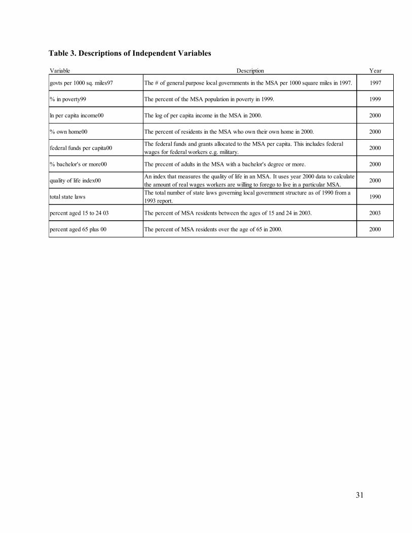
respectively. Table 3 (page 31) provides a list of the independent variables and a description for

each one. The economic freedom measures were constructed using data from 2002.

Because many of the control variables are likely affected by economic freedom, causality

may work in the reverse direction. For example, although the proportion of people in an MSA

with a bachelor’s degree or higher likely affects public policy and thus economic freedom, it may

also be the case that people with a bachelor’s or advanced degree are attracted to places with

more economic freedom. To reduce such endogeneity concerns, we have chosen to use data for

all of our regressors from years before 2002 because that is the year of the data used to construct

the economic freedom index.50 This strategy assumes, for example, that the proportion of people

with a bachelor’s or advanced degree in 2000 contributed to the MSA’s economic freedom score

in 2002, rather than the other way around. In general, we use data from the 2000 Census, but in

the case of our number of governments’ variables, the data we use are from the 1997 Census of

Governments (COG) because the next COG took place in 2002, the same year from which data

were used to construct the economic freedom indices. Thus, the use of the 1997 number of

governments reduces concerns of reverse causation. The two-digit number after the control

variable indicates the year of the data (e.g., 00 means the data are from 2000.)

There are 384 MSAs with measures of economic freedom from Stansel’s “Economic

Freedom Index,” which is our dependent variable.51 This index is modeled after the 2008 edition

50 The only exception is proportion of residents between the ages of 15 and 24. We could not locate accurate data for this age group in an earlier year, but the 2003 data should be strongly correlated with the 2002 or earlier data, and use of the former should not affect any of our results. 51 Stansel, “An Economic Freedom Index for U.S. Metropolitan Areas.”

14

of Economic Freedom of North America but aggregated at the MSA level rather than at the state

(or province) level.52 The three major categories are the same: size of government, takings and

discriminatory taxation, and labor market freedom.

Area 1, the size of government, contains three variables: (1) general consumption

expenditures by government as a percentage of personal income, (2) transfers and subsidies as a

percentage of personal income, and (3) social security payments as a percentage of personal income

(which at the state and local levels refers to social insurance and retirement payments). Area 2,

taxation, contains four variables: (1) total tax revenue as a percentage of personal income, (2) total

individual income tax revenue as a percentage of personal income, (3) indirect tax revenue as a

percentage of personal income, and (4) sales taxes collected as a percentage of personal income.

Areas 1 and 2 include the spending and revenue from all local governments within each county

contained in the MSA. The US Census Bureau provides such data in its Census of Governments,

performed every five years. It includes general-purpose governments—counties, municipalities, and

townships—as well as special-purpose governments—school districts and all other single-purpose

local governments. To facilitate comparisons across states with varying levels of fiscal

decentralization, a state average for state-level taxes and spending is added to that local number.

Area 3, labor market freedom, contains three variables: (1) minimum wage annual

income as a percentage of MSA per capita personal income, (2) state and local government

employment as a percentage of total employment, and (3) state union density (aggregated at the

state level because of limited availability of local-level data). The values for each of those 10

variables are standardized so that the most free receives a score of 10, the least free receives a

score of 0, and all others fall proportionately between 0 and 10. In each of the three areas, the

52 Amela Karabegović and Fred McMahon, Economic Freedom of North America: 2008 Annual Report (Vancouver, BC: The Fraser Institute, 2008).

15

average of the variables is calculated. Those three area scores are then averaged to produce the

overall economic freedom score for each of the 384 separate MSAs. There is wide dispersion in

the index, and in general, it is positively correlated with positive economic outcomes (as have the

national-level and state-level indices).53

Our measure of the intensity of local government competition, which is our key

independent variable, is the number of general-purpose54 local governments per 1,000 square miles

(from the 1997 Census of Governments conducted by the US Census Bureau). This measure

captures the geographical proximity of these governments, whereas per capita measures may not.

We argue that within a particular MSA, geography is likely to be more important than absolute

population in determining political entities.55 This relative importance of geography is likely

because of the historical conglomerations of “neighborhoods” and may also be affected by school

districting, both of which are likely to influence relocation decisions. Additionally, the cost of

relocating to a new jurisdiction (voting with one’s feet), in terms of both actual expenditures and

lost social capital, is largely a function of distance. That cost is best captured by a measure of

53 Examples of other work using the MSA index include Jamie Bologna, Andrew T. Young, and Donald J. Lacombe, “A Spatial Analysis of Incomes and Institutional Quality: Evidence from US Metropolitan Areas,” Journal of Institutional Economics 12, no. 1 (2016): 191–216; Jamie Bologna, “A Spatial Analysis of Entrepreneurship and Institutional Quality: Evidence from U.S. Metropolitan Areas,” Journal of Regional Analysis and Policy 44, no. 2 (2015): 109–31; James V. Koch, “Why Do People Move from One Metropolitan Area to Another?,” in Economic Behavior, Economic Freedom, and Entrepreneurship, ed. Richard Cebula, Joshua C. Hall, Franklin G. Mixon Jr., and James E. Payne (Cheltenham, UK: Edward Elgar Publishing, 2015), 145–60; and Crystal Wong and Dean Stansel, “An Exploratory Empirical Note on the Relationship between Local Labor Market Freedom and the Female Labor Force Participation Rate in US Metropolitan Areas,” Empirical Economics Letters 15, no. 11 (2016). 54 General-purpose local governments include only counties, municipalities, and townships. Single-purpose governments, such as school and water districts, within an individual metro area generally do not compete with each other (because they have different purposes) and they sometimes overlap. 55 In preliminary work, we also used the number of local governments per 100,000 people as an alternative measure of the intensity of local government competition. This variable does not capture geographic proximity, which can affect location decisions. In fact, the correlation between the two measures is 0.46, which is evidence that they are not measuring the same thing. The regressions using the number of local governments per 100,000 people were not statistically significant across any model’s specification. Regressions using the alternative measure of local government competition are available upon request.

16

governments’ geographic proximity. Our a priori expectation, based on the Leviathan hypothesis,

is that the number of local governments per 1,000 square miles variable will exhibit positive signs.

We know from firm location decision models that labor quality, human capital, labor

costs, employee stability, and market access matter.56 Given that individual relocation decisions

are strongly linked to employment, we use a handful of standard control variables. The control

variables are included to capture the characteristics of the MSAs’ populations that could affect

local institutions and thus economic freedom. The percentage of people in poverty in an MSA

and the MSA’s average per capita income can affect the desire for local redistribution.

Homeowners are likely to be more tied to an area and have longer time horizons when it comes

to local politics, so MSAs with a larger percentage of homeowners may have different local

institutions. Educated people and elderly people are more likely to vote and influence local

politics, so variation in those factors across MSAs can affect economic freedom. The “federal

funds per capita” variable serves to capture intergovernmental transfers from the national to the

MSA level. The number of state laws governing local government structure affects the ability of

local governments to tax and regulate their residents, an ability that can affect economic

freedom. And finally, places with a better quality of life because of climate and geography may

be able to have lower economic freedom, ceteris paribus, because better climate serves as a form

of compensating differential.

56 Peter Doeringer, Christine Evans-Klock, and David Terkla, “What Attracts High Performance Factories? Management Culture and Regional Advantage,” Regional Science and Urban Economics 34, no. 5 (2004): 591–618; Stephan J. Goetz, “State- and County-Level Determinants of Food Manufacturing Establishment Growth: 1987–93,” American Journal of Agricultural Economics 79, no. 3 (1997): 838–50; Paulo Guimarães, Octávio Figueirdo, and Douglas Woodward, “A Tractable Approach to the Firm Location Decision Problem,” Review of Economics and Statistics 85, no. 1 (2003): 201–4; Leslie E. Papke, “Interstate Business Tax Differentials and New Firm Location: Evidence from Panel Data,” Journal of Public Economics 45, no. 1 (1991): 47–68; Michael Wasylenko, “Taxation and Economic Development: The State of the Economic Literature,” New England Economic Review (March–April 1997): 37–52.

17

Percentage of adults with a bachelor’s degree or more, percentage of people who own

their own home, percentage of people in poverty, per capita income, and federal funds per capita

come from the 2006 State and Metropolitan Area Data Book published by the US Census

Bureau. The data themselves are from the year 2000. The number of state laws governing local

government structure is from a US Advisory Council on Intergovernmental Relations report.57

This measure is a count of state laws from 1990.

The quality-of-life measure comes from an index created by Yong Chen and Stuart S.

Rosenthal.58 This relative measure is determined by “the amount of real wage workers are

willing to forgo for the opportunity to locate in the more attractive area.” The index is

constructed through hedonic modeling for each particular MSA. Other variables are often used to

measure an MSA’s amenities, such as average January temperature, which partially captures

climate amenities only, and proportion of employment in accommodations, which indirectly

measures an area’s appeal on the basis of the proportion of its labor resources devoted to

tourism. Instead, we use the quality-of-life index (life index) in our primary specification. We

contend that it more directly measures an area’s amenities by calculating how much a person is

willing to pay in the form of forgone wages to live in a particular place.

Chen and Rosenthal provide indexes for 1970, 1980, 1990, and 2000; we employ the

2000 index. Unfortunately, the quality-of-life index by MSA is available for only 268 of the

MSAs,59 so only 268 of our observations have nonmissing values for all of the independent and

dependent variables.

57 US Advisory Commission on Intergovernmental Relations, State Laws Governing Local Government Structure and Administration, March 1993. 58 Yong Chen and Stuart S. Rosenthal, “Local Amenities and Life-Cycle Migration: Do People Move for Jobs or Fun?,” Journal of Urban Economics 64, no. 3 (2008): 519–37. 59 Ibid.

18

Because the quality-of-life index is missing for 100 observations, table 1 contains the

averages and standard errors of the dependent and independent variables for the entire dataset,

whereas table 2 contains the same measures for only the MSAs for which the life index variable

is available. A comparison of the two tables shows that the 100 MSAs without a life index score

are located across all the census divisions and that their omission does not substantially alter the

average values of any of the dependent or independent variables. We check our preferred result

with robustness checks using alternative measures of quality of life. The robustness checks yield

similar results, so we are confident that using the life index to capture an MSA’s amenities in our

preferred specification does not bias our results.60

Our hypothesis is that having more local governments in an MSA will have a positive

effect on MSA economic freedom because actual and potential exit restricts local government’s

ability to extract resources from and impose constraints on citizens. The MSA is an appropriate

unit of analysis for examining local government competition because most relocation takes place

within an MSA. According to recent migration data from the US Census, 64 percent of the 35.9

million people who moved between 2012 and 2013 remained within the same county (ergo, the

same MSA.) Another 13 percent (4.7 million people) made intercounty moves of less than 50

miles.61 Thus, most of the intranational migration in the United States—almost 78 percent—is

relatively local and likely within the same MSA. This is evidence that the relevant location

choice set facing citizens largely consists of various local government jurisdictions within the

same MSA rather than jurisdictions across MSAs.

60As a robustness check, we estimate the model using two common alternative measures of an MSA’s place-specific amenities: average January temperature and proportion of private employment in the accommodations industry. These measures are available for 373 and 350 MSAs, respectively, and the results are available upon request. The point estimates for the number of governments per 100,000 square miles are consistent with the model using the life index. Later we show that using average January temperature in a regression that includes MSAs only in the Northeast, Midwest, and West regions also does not significantly affect the results (see table 9). 61 David Ihrke, “Reasons for Moving: 2012 to 2013,” US Census Bureau, June 2014.

19

3. Regression Results

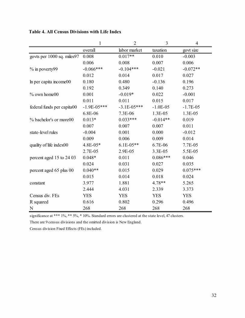
Table 4 (page 32) contains the results from running the complete model. In this specification, the

number of local governments has a statistically significant relationship only with labor market

freedom (column 2). The point estimate is positive but statistically insignificant for the overall

regression and the tax freedom regression, whereas it is negative and insignificant for the size of

government regression (column 4). These effects, which are statistically significant on labor

markets but not on the size of government and taxation, are similar to Mitchell and Stratmann’s

findings for overlapping tax jurisdictions.62

Areas with higher poverty rates have lower scores for overall economic freedom, labor

market freedom, and size of government, perhaps because areas with higher poverty rates tend to

have governments that spend more. Federal funds per capita also has a negative relationship with

overall economic freedom and labor market freedom. One explanation for this result is that

higher levels of federal funding reduce an area’s reliance on local tax revenue and thus reduce

the incentive to implement local policies that generate economic growth. The quality-of-life

index has a positive and significant association with labor market freedom and a positive but

marginally significant association with overall freedom.

The proportion of adults with a bachelor’s degree or more has a positive and statistically

significant relationship with overall freedom and labor market freedom, but it has a negative and

statistically significant relationship with taxation freedom. One explanation is that better-

educated residents value local government goods and services more than less-educated residents

do and are thus willing to pay more local taxes. If local government goods such as police and fire

62 Mitchell and Stratmann, “Tragedy of the Anticommons.”

20

protection are normal goods, then we might expect more educated residents with higher average

incomes will have a higher willingness to pay as well.

To get a better idea of the impact of an increase in the number of local governments per

square mile on labor market freedom, we calculate how an increase of one standard deviation in

the “number of governments” variable would affect labor market freedom. The sample standard

deviation of the number of local governments is 20.95, which means that an increase of one

standard deviation would increase labor market freedom by 0.36 points.63 This is about one-third

of the standard deviation of labor market freedom (1.15). A 0.36 increase in labor market freedom

is about equal to increasing Chicago’s labor market freedom (6.26) to that of Cincinnati (6.60).

3A. Regional Results

Next we run separate regressions by region to ascertain regional heterogeneity. This analysis has

a theoretical motivation, as explained by William A. Fischel.64 In the South and arid West

regions, Fischel finds that local government power is more concentrated in county governments

than in the denser Northeast and Midwest regions, largely because of rainfall and historical race-

based segregation.

In rainy areas that are relatively flat, population densities in the 19th and 20th centuries

were high enough to warrant forming many local governments. In such areas, the city or village

government had most of the power, and county governments, which are the states’ local

administrative units, played a relatively minor role, a relationship that continues to this day. As

63 The standard deviation can be calculated by multiplying the standard error in table 2 (1.28) by the square root of the number of observations (268); e.g., 1.28× 268 = 20.95. 64 William A. Fischel, Making the Grade: The Economic Evolution of American School Districts (Chicago: University of Chicago Press, 2009); William A. Fischel, Zoning Rules!: The Economics of Land Use Regulation (Cambridge, MA: Lincoln Institute of Land Policy, 2015).

21

the urban population spread out in the mid-20th century, the small rural towns in the North

became suburbs, each with its own distinct local government.

In more arid and mountainous areas such as western California, Arizona, Nevada, Utah,

and Colorado, populations were more scattered. To achieve economies of scale in the provision

of government goods and services (school districts, fire districts, and so on) with such sparse

populations, local government had to cover more area. Thus, the larger county, not a smaller

local government, became more influential in local governance in these areas.

The South is similar to the arid West because of racial segregation. As stated in Fischel,

“separate but equal” government services required local government jurisdictions that covered a

wide area in order to be economical.65 So, to maintain black-white segregation, more power was

allocated to the state and the state’s local administrative unit, the county. Because of this history,

local government in the South is more similar to the arid West than to the North, despite the

South’s having terrain and rainfall similar to the North.

Because of the differences in the intensity of local government power at the city (or

village) and county level that these historical and geographic factors created, we estimate four

separate regional regressions. Table 5 (page 33) shows the results for a regression that includes

the New England, Mid-Atlantic, East North Central, and West North Central divisions. Together

these divisions compose the Northeast and Midwest regions of the country (the North.) (Figure 1

provides a map that depicts the locations of the census divisions, and division Fixed Effects

(FEs) are included in the regressions.)

In this regional subsample, our results are largely consistent with theory. The number of

governments has a statistically significant relationship with overall, labor market, and taxation

65 Fischel, Making the Grade; Fischel, Zoning Rules!

22

freedom. An interesting result is that in states with more laws governing local government

structure, economic freedom is lower across all measures and statistically significant for three

out of four, the exception being taxation.

Again, to get a better idea of the impact of the number of local governments per square

mile, we calculate how an increase of one standard deviation in the “number of governments”

variable would affect overall economic freedom. The standard deviation of number of local

governments is 18.4 in the Midwest and Northeast regions.66 So an increase of one standard

deviation is associated with a 0.22 point increase in overall economic freedom, which is a little

less than one-third of the standard deviation of overall economic freedom in these regions (0.71).

As an example, a 0.22 increase would increase the overall economic freedom of Ocean City,

New Jersey (5.40), to roughly that of Dayton, Ohio (5.66).

Table 6 (page 34) displays the results from a regression that examines MSAs in only the

West South Central, East South Central, and South Atlantic divisions (the South). In this region

of the country, the number of local governments has no statistically significant relationship with

any measure of economic freedom, and the point estimates have a negative sign, which is

inconsistent with the Leviathan hypothesis.

Finally, table 7 (page 35) looks at the Mountain and Pacific Census Divisions (the West).

The number of governments per 100,000 square miles has a positive but statistically insignificant

relationship with each of the freedom measures.

With respect to the Leviathan hypothesis, only the Southern region of the country is

vastly inconsistent with the theory. Not only is the number of competing governments

66 The standard error for governments per 100,000 square miles for this subsample is 1.80, so the sample standard deviation is calculated as 1.80× 105 = 18.4.

23

statistically insignificant across all measures of economic freedom in the Southern MSAs, but the

coefficients also have the wrong sign.

Because of the South’s history of racial segregation and that history’s subsequent effects

on local government, in table 8 (page 36) we combine the Northeast, Midwest, and West regions

and leave out the South region (West South Central, East South Central, and South Atlantic

divisions). The regressions were run with all of the regressors in the model, but we omitted them

from the table to focus on the “number of local governments” coefficient. As shown in the table,

the coefficient is positive and significant at the 10 percent level in the overall freedom column

and at the 5 percent level in the labor market freedom column.

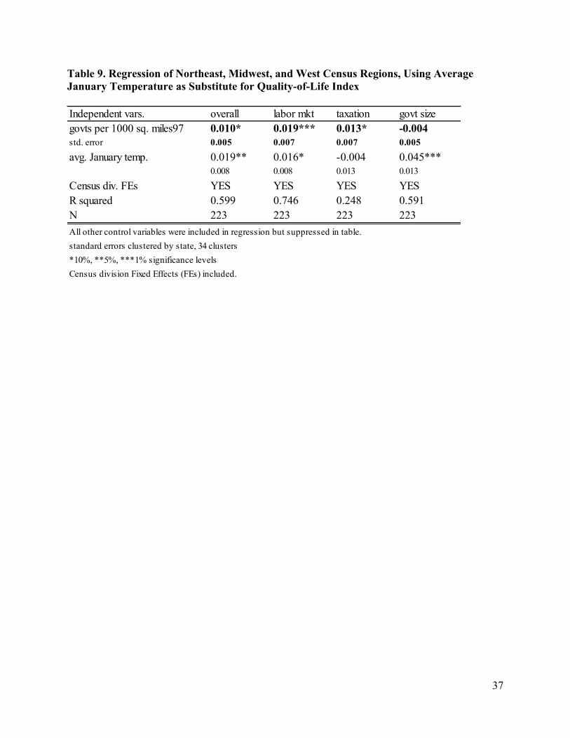
As mentioned previously, use of the quality-of-life index variable to control for climate

and geographic features limits our overall dataset to 268 observations. To test whether this

reduction in observations has an effect on the Leviathan-consistent results in the Northeast,

Midwest, and West regions, we estimate the regressions using an alternative climate control

variable, average January temperature. With this alternative measure, the number of observations

increases from 161 to 223. The results of this robustness check are in table 9 (page 37).

In table 9, the number of local governments control is still positive and statistically

significant at the 5 percent level for labor market freedom and the 10 percent level for overall

freedom and taxation freedom. Also, average January temperature has a positive and statistically

significant relationship at the 10 percent level or better for three of the four dependent variables,

the exception being taxation freedom. The signs on January temperature are qualitatively

consistent with those on the quality-of-life index in table 8, a finding which suggests that the two

variables are capturing similar relationships.67

67 But the two variables do not capture the exact same thing: the correlation coefficient between average January temperature and the quality-of-life index is 0.38.

24

These results are aligned with previous findings on the Leviathan hypothesis—namely,

that they are mixed. There is relatively strong evidence for the Leviathan hypothesis in the

North, weaker evidence in the arid West, and no evidence in the South. The historical structure

of local governance may explain some of this variation, but further research is needed before we

can make any firm conclusions.

Another reason we may see this result is unique to the study of metropolitan areas and

states. Both local and state political entities operate under the umbrella of wide-ranging, and

expansive, institutional rules and constraints at the federal level. It is certainly plausible that

institutional variations at state and local levels are simply being swamped by the federal-level

institutional framework.

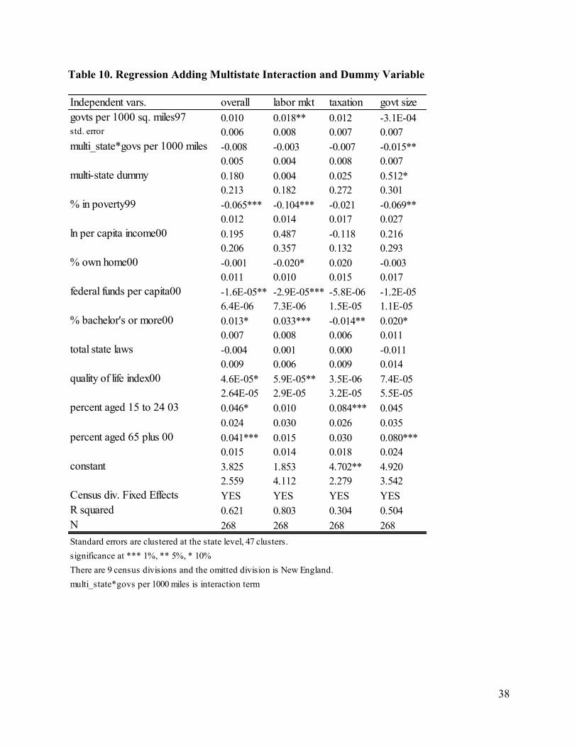
3B. MSAs That Cross State Borders

Some MSAs cross state borders, and this extra layer of government could have an effect on our

results because it affects the cost of intra-MSA migration. To see if there is any difference

between MSAs that are completely within one state and those that cross state borders, we added

a dummy variable that equals 1 if an MSA crosses state borders and 0 otherwise. We also

interacted this dummy variable with the “number of local governments” regressor to check for

effects on how the number of local governments affects economic freedom in an MSA when the

MSA contains multiple state governments. These results are presented in table 10 (page 38).

Adding the dummy and interaction term has a significant effect only on government size

(last column of table 10). If the MSA crosses state borders, the more competing local

governments within the MSA, the lower the “government size” economic freedom score. But the

dummy variable itself is positive and significant at the 10 percent level, and using the

25

magnitudes of the two coefficients, it would take about 30 additional governments to actually

decrease the “government size” score. The point estimates for these variables in the other

regressions are not statistically significant, nor does their inclusion significantly alter the point

estimates on the number of local governments from those of the original model in table 4.

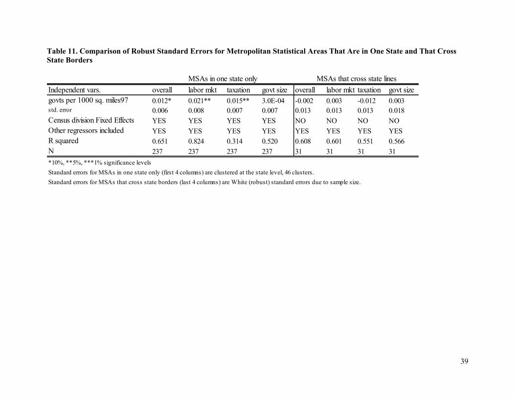
We also ran two separate regressions, one for MSAs that are contained within one state’s

borders and another for MSAs that cross state borders (table 11, page 39). Only 31 of the latter

also have all of the control variables, so drawing strong conclusions from this regression is not

recommended. The results for the 237 MSAs that are located within one state are similar in

magnitude to the original results in table 4, though the coefficient for the “number of local

governments” variable is now significant at the 10 percent level for overall freedom and the 5

percent level for taxation freedom. The coefficients on the number of local governments for the

sample of MSAs that cross state borders (columns 5–8) are generally close to zero and have large

standard errors, which is unsurprising given the small sample size.

This analysis indicates that including MSAs that cross state borders does not appear to

have a notable impact on our main results. Because we have no strong theoretical reason for

omitting such MSAs from our analysis, we prefer the overall results in table 4 and the regional

results in tables 5 through 9.

4. Conclusion

Hundreds of papers by independent researchers have found economic freedom to be positively

associated with good outcomes of all kinds. We instead investigate the determinants of that

economic freedom. In so doing, we provide a test of Brennan and Buchanan’s Leviathan

hypothesis, which states that “the potential for fiscal exploitation varies inversely with the

26

number of competing governmental units in the inclusive territory.”68 When we examine

metropolitan areas across the entire United States, we find mixed support for that hypothesis.

When we examine regional subsets of the data, we find that the hypothesis is generally supported

in all regions except the South. Further research is needed to determine the reasons for this

regional disparity.

68 Brennan and Buchanan, Power to Tax, 211.

27

Appendix: Tables

Table 1. Variable Averages and Standard Errors for Entire Dataset

0 1 2 3 4 5 6 7 8 9Dependent vars. Total N. Eng. Mid. Atl. E.N.C. W.N.C. S. Atl. E.S.C. W.S.C. Mtn. Pac.overall freedom 6.68 6.81 6.02 6.41 6.99 7.25 6.87 7.07 6.95 5.62std. error 0.04 0.16 0.15 0.07 0.10 0.08 0.12 0.10 0.11 0.11

labor market freedom 6.46 6.66 5.49 5.95 6.96 7.41 6.70 7.01 6.94 4.850.06 0.16 0.20 0.09 0.12 0.09 0.13 0.14 0.13 0.17

taxation freedom 6.06 5.83 5.25 5.77 6.08 6.33 6.70 6.27 6.11 6.010.04 0.22 0.20 0.07 0.10 0.08 0.17 0.12 0.12 0.09

size-of-govt freedom 7.51 7.93 7.32 7.50 7.93 8.00 7.21 7.94 7.79 6.000.06 0.17 0.10 0.14 0.12 0.13 0.17 0.10 0.14 0.19

N 384 18 34 63 32 81 30 43 35 48

Independent vars. Total N. Eng. Mid. Atl. E.N.C. W.N.C. S. Atl. E.S.C. W.S.C. Mtn. Pac.# of govts/1000 sq. miles 20.37 31.60 51.36 42.60 28.02 10.95 9.69 8.33 3.70 5.68std. error 1.04 2.82 4.30 1.49 2.34 1.08 1.45 0.79 0.68 0.88

# of govts/100K people 11.07 11.09 16.33 19.67 31.23 5.56 8.15 6.18 5.66 2.880.66 2.53 1.62 1.27 4.62 0.60 2.06 0.63 0.91 0.29

% in poverty99 12.08 8.79 10.35 9.60 9.69 12.58 13.99 16.46 12.07 13.200.22 0.55 0.48 0.31 0.42 0.38 0.49 0.85 0.66 0.66

ln per capita income00 10.2 10.4 10.3 10.2 10.2 10.2 10.1 10.1 10.1 10.20.01 0.06 0.03 0.02 0.02 0.02 0.02 0.03 0.04 0.06

% own home00 61.78 59.31 61.84 65.87 63.62 61.27 63.66 59.49 62.37 57.380.30 0.95 1.46 0.59 1.06 0.59 0.69 0.62 0.89 0.66

federal funds per capita00 5577.2 5804.0 6738.8 4515.5 5247.5 5807.5 7331.1 5196.0 5429.8 5273.8181.87 310.73 1267.88 165.19 251.04 288.52 1362.42 238.91 372.30 276.00

% bachelor's or more00 22.80 29.20 23.67 21.52 26.61 21.91 19.93 19.77 25.41 23.540.39 1.81 1.29 0.88 1.42 0.84 0.91 0.81 1.34 1.26

total state laws 89.15 65.89 92.41 92.70 89.72 86.19 85.87 87.05 96.31 94.170.69 3.28 1.04 1.49 1.26 1.83 2.03 1.75 2.25 1.23

proportion 15 to 24_03 15.11 13.54 14.46 15.02 16.56 14.62 14.79 15.88 15.63 15.30.14 0.35 0.57 0.3 0.63 0.34 0.38 0.33 0.39 0.27

proportion 65 plus_00 12.66 13.77 14.52 12.67 12 13.91 12.14 11.53 11.86 11.210.18 0.7 0.43 0.23 0.34 0.61 0.36 0.38 0.63 0.34

life index00* -37.8 -345.1 -1313.0 -1459.6 -326.7 230.0 -375.8 -123.4 1215.7 2203.3122.08 737.07 252.03 178.53 258.27 212.31 212.29 222.53 261.29 487.20

N 376 16 34 63 29 79 30 43 34 48notes: Life index N is 268, 10, 26, 47, 22, 53, 22, 33, 20, and 36 respectively

Table 1 - Variable average and standard errors for entire data set

28

Table 1 (continued)





N 384 18 34 63 32 81 30 43 35 48


# of govts/100K people 11.07 11.09 16.33 19.67 31.23 5.56 8.15 6.18 5.66 2.880.66 2.53 1.62 1.27 4.62 0.60 2.06 0.63 0.91 0.29

% in poverty99 12.08 8.79 10.35 9.60 9.69 12.58 13.99 16.46 12.07 13.200.22 0.55 0.48 0.31 0.42 0.38 0.49 0.85 0.66 0.66


% own home00 61.78 59.31 61.84 65.87 63.62 61.27 63.66 59.49 62.37 57.380.30 0.95 1.46 0.59 1.06 0.59 0.69 0.62 0.89 0.66



total state laws 89.15 65.89 92.41 92.70 89.72 86.19 85.87 87.05 96.31 94.170.69 3.28 1.04 1.49 1.26 1.83 2.03 1.75 2.25 1.23

proportion 15 to 24_03 15.11 13.54 14.46 15.02 16.56 14.62 14.79 15.88 15.63 15.30.14 0.35 0.57 0.3 0.63 0.34 0.38 0.33 0.39 0.27

proportion 65 plus_00 12.66 13.77 14.52 12.67 12 13.91 12.14 11.53 11.86 11.210.18 0.7 0.43 0.23 0.34 0.61 0.36 0.38 0.63 0.34

life index00* -37.8 -345.1 -1313.0 -1459.6 -326.7 230.0 -375.8 -123.4 1215.7 2203.3122.08 737.07 252.03 178.53 258.27 212.31 212.29 222.53 261.29 487.20

N 376 16 34 63 29 79 30 43 34 48notes: Life index N is 268, 10, 26, 47, 22, 53, 22, 33, 20, and 36 respectively

Table 1 - Variable average and standard errors for entire data set

29

Table 2. Variable Averages and Standard Errors, Life Index Available





N 268 10 26 47 22 52 22 33 20 36


# of govts/100K people 10.45 6.45 17.09 19.51 28.15 4.05 8.92 5.77 3.50 2.470.72 1.10 2.04 1.49 3.86 0.41 2.71 0.65 0.71 0.26

% in poverty99 12.18 8.71 10.60 9.99 9.49 12.21 14.32 16.74 12.13 13.290.26 0.64 0.54 0.34 0.46 0.47 0.63 1.06 0.95 0.75


% own home00 61.40 59.06 62.43 64.65 64.61 60.31 63.10 59.85 61.20 57.200.33 1.45 1.44 0.60 1.03 0.70 0.74 0.65 1.23 0.73



total state laws 89.74 65.40 92.53 92.79 88.77 89.38 82.68 88.33 95.10 94.220.82 4.67 1.09 1.81 1.51 2.43 2.07 2.21 3.00 1.37

proportion 15 to 24_03 14.99 13.14 14.23 15.34 15.73 14.41 14.86 15.7 15.4 15.20.14 0.48 0.52 0.38 0.49 0.41 0.47 0.21 0.47 0.28

proportion 65 plus_00 12.49 14.25 14.64 12.48 12.19 13.74 12.11 11.06 10.92 11.250.2 1.05 0.44 0.26 0.4 0.75 0.44 0.34 0.66 0.35

life index00 -37.8 -345.1 -1313.0 -1459.6 -326.7 230.0 -375.8 -123.4 1215.7 2203.3122.1 737.1 252.0 178.5 258.3 212.3 212.3 222.5 261.3 487.2

N 268 10 26 47 22 52 22 33 20 36

Table 2 - Variable averages and standard errors - life index available

30

Table 2 (continued)





N 268 10 26 47 22 52 22 33 20 36


# of govts/100K people 10.45 6.45 17.09 19.51 28.15 4.05 8.92 5.77 3.50 2.470.72 1.10 2.04 1.49 3.86 0.41 2.71 0.65 0.71 0.26

% in poverty99 12.18 8.71 10.60 9.99 9.49 12.21 14.32 16.74 12.13 13.290.26 0.64 0.54 0.34 0.46 0.47 0.63 1.06 0.95 0.75


% own home00 61.40 59.06 62.43 64.65 64.61 60.31 63.10 59.85 61.20 57.200.33 1.45 1.44 0.60 1.03 0.70 0.74 0.65 1.23 0.73



total state laws 89.74 65.40 92.53 92.79 88.77 89.38 82.68 88.33 95.10 94.220.82 4.67 1.09 1.81 1.51 2.43 2.07 2.21 3.00 1.37

proportion 15 to 24_03 14.99 13.14 14.23 15.34 15.73 14.41 14.86 15.7 15.4 15.20.14 0.48 0.52 0.38 0.49 0.41 0.47 0.21 0.47 0.28

proportion 65 plus_00 12.49 14.25 14.64 12.48 12.19 13.74 12.11 11.06 10.92 11.250.2 1.05 0.44 0.26 0.4 0.75 0.44 0.34 0.66 0.35

life index00 -37.8 -345.1 -1313.0 -1459.6 -326.7 230.0 -375.8 -123.4 1215.7 2203.3122.1 737.1 252.0 178.5 258.3 212.3 212.3 222.5 261.3 487.2

N 268 10 26 47 22 52 22 33 20 36

Table 2 - Variable averages and standard errors - life index available

31

Table 3. Descriptions of Independent Variables

Variable Description Year

govts per 1000 sq. miles97 The # of general purpose local governments in the MSA per 1000 square miles in 1997. 1997

% in poverty99 The percent of the MSA population in poverty in 1999. 1999

ln per capita income00 The log of per capita income in the MSA in 2000. 2000

% own home00 The percent of residents in the MSA who own their own home in 2000. 2000

federal funds per capita00The federal funds and grants allocated to the MSA per capita. This includes federal wages for federal workers e.g. military.

2000

% bachelor's or more00 The precent of adults in the MSA with a bachelor's degree or more. 2000

quality of life index00An index that measures the quality of life in an MSA. It uses year 2000 data to calculate the amount of real wages workers are willing to forego to live in a particular MSA.

2000

total state lawsThe total number of state laws governing local government structure as of 1990 from a 1993 report.

1990

percent aged 15 to 24 03 The percent of MSA residents between the ages of 15 and 24 in 2003. 2003

percent aged 65 plus 00 The percent of MSA residents over the age of 65 in 2000. 2000

Table 3 - Descriptions of independent variables

32

Table 4. All Census Divisions with Life Index

1 2 3 4overall labor market taxation govt size

govts per 1000 sq. miles97 0.008 0.017** 0.010 -0.0030.006 0.008 0.007 0.006

% in poverty99 -0.066*** -0.104*** -0.021 -0.072**0.012 0.014 0.017 0.027

ln per capita income00 0.180 0.480 -0.136 0.1960.192 0.349 0.140 0.273

% own home00 0.001 -0.019* 0.022 -0.0010.011 0.011 0.015 0.017

federal funds per capita00 -1.9E-05*** -3.1E-05*** -1.0E-05 -1.7E-056.8E-06 7.3E-06 1.3E-05 1.3E-05

% bachelor's or more00 0.013* 0.033*** -0.014** 0.0190.007 0.007 0.007 0.011

state-level rules -0.004 0.001 0.000 -0.0120.009 0.006 0.009 0.014

quality of life index00 4.8E-05* 6.1E-05** 6.7E-06 7.7E-052.7E-05 2.9E-05 3.3E-05 5.5E-05

percent aged 15 to 24 03 0.048* 0.011 0.086*** 0.0460.024 0.031 0.027 0.035

percent aged 65 plus 00 0.040** 0.015 0.029 0.075***0.015 0.014 0.018 0.024

constant 3.977 1.881 4.78** 5.2652.444 4.031 2.339 3.373

Census div. FEs YES YES YES YESR squared 0.616 0.802 0.296 0.496N 268 268 268 268significance at *** 1%, ** 5%, * 10%. Standard errors are clustered at the state level, 47 clusters.

There are 9 census divisions and the omitted division is New England.

Census division Fixed Effects (FEs) included.

33

Table 5. Robust Standard Errors—New England, Mid-Atlantic, East North Central, and West North Central Census Divisions

Independent vars. overall labor mkt taxation govt sizegovts per 1000 sq. miles97 0.012*** 0.021*** 0.014*** 0.001std. error 0.004 0.005 0.005 0.004

% in poverty99 0.021 -0.080 0.130** 0.0150.043 0.049 0.055 0.050

ln per capita income00 0.299 2.987** -1.503 -0.5851.082 1.197 1.679 1.337

% own home00 0.018 -0.013 0.058* 0.0100.022 0.029 0.033 0.025

federal funds per capita00 -3.8E-05*** -4.5E-05*** -3.3E-05 -3.7E-05**1.5E-05 1.7E-05 2.1E-05 1.7E-05

% bachelor's or more00 0.008 -0.024 0.022 0.0240.023 0.023 0.028 0.031

total state laws -0.023*** -0.012** -0.010 -0.048***0.006 0.006 0.007 0.010

quality of life index00 1.2E-04* 2.4E-04*** 5.8E-05 6.2E-056.2E-05 6.6E-05 8.5E-05 7.5E-05

percent aged 15 to 24 03 0.001 0.071 -0.041 -0.0250.066 0.068 0.081 0.082

percent aged 65 plus 00 -0.029 -0.032 -0.038 -0.0190.050 0.039 0.063 0.068

constant 3.95 -22.49 17.85 16.5012.123 13.690 19.115 14.353

Census div. FEs YES YES YES YESR squared 0.420 0.591 0.344 0.392N 105 105 105 105robust standard errors*10%, **5%, ***1% significance levelsCensus division Fixed Effects (FEs) included.

34

Table 6. Robust Standard Errors—South Atlantic, East South Central, and West South Central Census Divisions

Independent vars. overall labor mkt taxation govt sizegovts per 1000 sq. miles97 -0.009 -0.007 -0.015 -0.006std. error 0.007 0.007 0.012 0.010

% in poverty99 -0.033 -0.032* -0.022 -0.045std. error 0.024 0.017 0.038 0.036

ln per capita income00 1.388* 3.498*** 0.075 0.5920.788 0.531 1.180 1.150

% own home00 -0.003 -0.006 0.010 -0.0140.021 0.011 0.030 0.033

federal funds per capita00 -7.65E-06 -2.1E-05** -1.3E-05 1.0E-059.4E-06 7.9E-06 2.0E-05 1.1E-05

% bachelor's or more00 0.000 0.002 -0.013 0.0110.012 0.010 0.018 0.019

total state laws -4.7E-04 0.004 -0.006 0.0010.005 0.003 0.007 0.006

quality of life index00 8.2E-05 1.2E-04*** 8.4E-05 3.9E-056.1E-05 4.7E-05 9.2E-05 8.3E-05

percent aged 15 to 24 03 0.034 0.013 0.071 0.0160.033 0.023 0.047 0.047

percent aged 65 plus 00 0.030* -0.011 0.038 0.063***0.017 0.012 0.026 0.023

constant -7.16 -27.96*** 5.25 1.239.057 5.674 13.466 13.471


35

Table 7. Robust Standard Errors—Mountain and Pacific Census Divisions

Independent vars. overall labor mkt taxation govt sizegovts per 1000 sq. miles97 0.013 0.016 0.003 0.021std. error 0.013 0.012 0.024 0.037

% in poverty99 -0.106*** -0.102*** -0.045 -0.172***0.027 0.025 0.039 0.050

ln per capita income00 0.019 0.157* -0.115 0.0150.080 0.093 0.091 0.161

% own home00 -0.025 -0.030 0.013 -0.059*0.018 0.018 0.021 0.033

federal funds per capita00 -1.7E-05 -5.9E-05* 5.0E-05 -4.2E-053.1E-05 3.2E-05 4.7E-05 6.5E-05

% bachelor's or more00 0.005 0.042*** -0.018 -0.0090.014 0.013 0.018 0.021

total state laws 0.010 0.004 0.016 0.0100.007 0.009 0.012 0.018

quality of life index00 1.9E-05 1.1E-05 -5.4E-05 1.0E-04*2.6E-05 3.3E-05 4.5E-05 5.9E-05

percent aged 15 to 24 03 0.014 -0.057 0.004 0.0950.059 0.056 0.078 0.094

percent aged 65 plus 00 0.069*** 0.046* 0.003 0.159***0.024 0.023 0.054 0.056

constant 7.680** 7.743*** 5.726*** 9.570***1.478 1.670 2.098 3.000


36

Table 8. Regression of Northeast, Midwest, and West Census Regions

Independent vars. overall labor mkt taxation govt sizegovts per 1000 sq. miles97 0.013* 0.022** 0.013 0.003std. error 0.006 0.008 0.008 0.006

% in poverty99 -0.074** -0.115*** -0.001 -0.106*0.033 0.020 0.041 0.059

per capita income00 0.099 0.280 -0.134 0.1510.155 0.223 0.166 0.268

% own home00 -0.001 -0.020 0.033 -0.0150.017 0.015 0.020 0.027

federal funds per capita00 -3.3E-05*** -3.9E-05*** -1.8E-05 -4.3E-05**9.2E-06 8.8E-06 1.6E-05 1.7E-05

% bachelor's or more00 0.011 0.028** -0.008 0.0110.012 0.010 0.013 0.018

total state laws -0.012 -0.008 0.001 -0.0280.012 0.009 0.010 0.021

quality of life index00 4.3E-05 7.4E-05** -1.5E-05 7.1E-053.6E-05 3.5E-05 4.8E-05 5.7E-05

percent aged 15 to 24 03 0.048 0.012 0.069 0.0610.037 0.040 0.046 0.046

percent aged 65 plus 00 0.028 0.012 0.008 0.0660.025 0.027 0.037 0.039

constant 5.68*** 4.803 4.179 8.061**2.082 2.969 2.535 3.380

Census div. FEs YES YES YES YESR squared 0.567 0.753 0.243 0.524N 161 161 161 161standard errors clustered by state, 32 clusters*10%, **5%, ***1% significance levelsCensus division Fixed Effects (FEs) included.

37

Table 9. Regression of Northeast, Midwest, and West Census Regions, Using Average January Temperature as Substitute for Quality-of-Life Index

Independent vars. overall labor mkt taxation govt sizegovts per 1000 sq. miles97 0.010* 0.019*** 0.013* -0.004std. error 0.005 0.007 0.007 0.005

avg. January temp. 0.019** 0.016* -0.004 0.045***0.008 0.008 0.013 0.013

Census div. FEs YES YES YES YESR squared 0.599 0.746 0.248 0.591N 223 223 223 223All other control variables were included in regression but suppressed in table.standard errors clustered by state, 34 clusters*10%, **5%, ***1% significance levelsCensus division Fixed Effects (FEs) included.

38

Table 10. Regression Adding Multistate Interaction and Dummy Variable

Independent vars. overall labor mkt taxation govt sizegovts per 1000 sq. miles97 0.010 0.018** 0.012 -3.1E-04std. error 0.006 0.008 0.007 0.007multi_state*govs per 1000 miles -0.008 -0.003 -0.007 -0.015**

0.005 0.004 0.008 0.007multi-state dummy 0.180 0.004 0.025 0.512*

0.213 0.182 0.272 0.301% in poverty99 -0.065*** -0.104*** -0.021 -0.069**

0.012 0.014 0.017 0.027ln per capita income00 0.195 0.487 -0.118 0.216

0.206 0.357 0.132 0.293% own home00 -0.001 -0.020* 0.020 -0.003

0.011 0.010 0.015 0.017federal funds per capita00 -1.6E-05** -2.9E-05*** -5.8E-06 -1.2E-05

6.4E-06 7.3E-06 1.5E-05 1.1E-05% bachelor's or more00 0.013* 0.033*** -0.014** 0.020*

0.007 0.008 0.006 0.011total state laws -0.004 0.001 0.000 -0.011

0.009 0.006 0.009 0.014quality of life index00 4.6E-05* 5.9E-05** 3.5E-06 7.4E-05

2.64E-05 2.9E-05 3.2E-05 5.5E-05percent aged 15 to 24 03 0.046* 0.010 0.084*** 0.045

0.024 0.030 0.026 0.035percent aged 65 plus 00 0.041*** 0.015 0.030 0.080***

0.015 0.014 0.018 0.024constant 3.825 1.853 4.702** 4.920

2.559 4.112 2.279 3.542Census div. Fixed Effects YES YES YES YESR squared 0.621 0.803 0.304 0.504N 268 268 268 268Standard errors are clustered at the state level, 47 clusters.significance at *** 1%, ** 5%, * 10%There are 9 census divisions and the omitted division is New England.multi_state*govs per 1000 miles is interaction term

39

Table 11. Comparison of Robust Standard Errors for Metropolitan Statistical Areas That Are in One State and That Cross State Borders

Independent vars. overall labor mkt taxation govt size overall labor mkt taxation govt sizegovts per 1000 sq. miles97 0.012* 0.021** 0.015** 3.0E-04 -0.002 0.003 -0.012 0.003std. error 0.006 0.008 0.007 0.007 0.013 0.013 0.013 0.018Census division Fixed Effects YES YES YES YES NO NO NO NOOther regressors included YES YES YES YES YES YES YES YESR squared 0.651 0.824 0.314 0.520 0.608 0.601 0.551 0.566N 237 237 237 237 31 31 31 31*10%, **5%, ***1% significance levelsStandard errors for MSAs in one state only (first 4 columns) are clustered at the state level, 46 clusters.Standard errors for MSAs that cross state borders (last 4 columns) are White (robust) standard errors due to sample size.

MSAs in one state only MSAs that cross state lines

local governments and economic freedom - mercatus … · local governments and economic freedom ......

Documents