local and global indeterminacy in two-sector models of endogenous growth

Journal of Mathematical Economics 46 (2010) 893–911

Contents lists available at ScienceDirect

Journal of Mathematical Economics

journa l homepage: www.e lsev ier .com/ locate / jmateco

Local and global indeterminacy in two-sector models of endogenousgrowth�

Paulo Britoa, Alain Vendittib,∗

a ISEG - Technical University of Lisbon and UECE, Portugalb CNRS - GREQAM and EDHEC, 2 rue de la Charité, 13002 Marseille, France

a r t i c l e i n f o

Article history:Received 31 July 2009Received in revised form 2 August 2010Accepted 2 August 2010Available online 12 August 2010

JEL classification:C62E32O41

Keywords:Two-sector modelEndogenous growthEconomy-wide externalitiesLocal and global indeterminacyPovert traps

a b s t r a c t

We consider a two-sector endogenous growth model where the productions of the finalgood and human capital require economy-wide external effects. Assuming constant returnsto scale at the private and social levels, we show that local and global indeterminacy of equi-librium paths are compatible with any values for the elasticity of intertemporal substitutionin consumption and any sign for the capital intensity difference across the two sectors. Wealso show that for any value of the elasticity of intertemporal substitution in consumption,poverty traps may occur when the final good sector is capital intensive in human capital.

© 2010 Elsevier B.V. All rights reserved.

1. Introduction

This paper is concerned with the existence of multiple equilibria in two-sector models of endogenous growth witheconomy-wide external effects à la Romer (1986). Most of the papers on multiple equilibria available in the literature providea separate analysis of local versus global indeterminacy and give strong restrictions on technologies and/or preferences. Ouraim is then to develop a two-sector formulation in which the existence of local and global indeterminacy can be analysedsimultaneously and to provide less restrictive sufficient conditions than those usually available. Local indeterminacy isassociated with the existence of a continuum of equilibrium paths from different initial conditions converging towards agiven stationary balanced growth path, while global indeterminacy concerns the existence of multiple equilibrium pathsfrom a given initial condition converging towards different stationary balanced growth paths. Global indeterminacy is thenassociated with the existence of poverty traps.

� We thank E. Augeraud-Véron, R. Boucekkine, J.P. Drugeon, C. García-Penalosa, O. Licandro, P. Michel, K. Nishimura, M. Santos, P. Wang and twoanonymours referees for useful comments and suggestions. Financial supports by Fundacão para a Ciência e a Tecnologia (Project POCTI/eco/13028/98and Multi-annual Funding Project POCI/U0436/2006), Portugal, and by French National Research Agency Grant (ANR-08-BLAN-0245-01) are gratefullyacknowledged.

∗ Corresponding author. Tel.: +33 491140752; fax: +33 491900227.E-mail addresses: [email protected] (P. Brito), [email protected] (A. Venditti).

0304-4068/$ – see front matter © 2010 Elsevier B.V. All rights reserved.doi:10.1016/j.jmateco.2010.08.003

dx.doi.org/10.1016/j.jmateco.2010.08.003

http://www.sciencedirect.com/science/journal/03044068

http://www.elsevier.com/locate/jmateco

mailto:[email protected]

mailto:[email protected]

dx.doi.org/10.1016/j.jmateco.2010.08.003

894 P. Brito, A. Venditti / Journal of Mathematical Economics 46 (2010) 893–911

The existence of local indeterminacy and multiple converging balanced growth paths have been a major concern ofthe literature dealing with two-sector endogenous growth models. Depending on the assumptions on the externalities,different types of conclusions have been provided. Benhabib and Perli (1994) and Xie (1994) consider the Lucas (1988)formulation with aggregate human capital externalities in the final good sector only. They prove the uniqueness of thestationary balanced growth path and show that the existence of local indeterminacy requires a large enough elasticity ofintertemporal substitution in consumption.1Benhabib et al. (2000), Mino (2001) and Nishimura and Venditti (2004) considersector-specific externalities in both sectors. Uniqueness of the stationary balanced growth path is also obtained and localindeterminacy arises under conditions on the capital intensity difference across sectors, namely if the final good sector ismore physical capital intensive from the social perspective but more human capital intensive from the private perspectivethan the human capital sector.2 It is worth noting that no particular condition on the elasticity of intertemporal substitutionin consumption is necessary in this case.

Concerning the existence of multiple stationary balanced growth paths, an augmented version of the Lucas model is usu-ally considered. In a first set of contributions we find Benhabib and Perli (1994) and Ladrón-de-Guevara et al. (1997, 1999)who introduce endogenous leisure to obtain two stationary solutions. In a second and more recent set of contributions,García-Belenguer (2007) and Mattana et al. (2009) focus on different specifications for the external effects. García-Belenguer(2007) shows the existence of multiple stationary balanced growth paths with a Lucas model augmented to include aggregatephysical capital externalities in the production of the final good and decreasing returns to scale in the human capital accumu-lation process. Local indeterminacy and poverty traps through the existence of global indeterminacy are also obtained butrequire the elasticity of intertemporal substitution in consumption to be larger than one.3 In Mattana et al. (2009), multiplestationary balanced growth paths are derived from the introduction of externalities in the human capital sector, and globalindeterminacy is exhibited through an homoclinic bifurcation.

In this paper, we develop a formulation which allows to provide a joint analysis of multiple stationary balanced growthpaths and multiple competitive equilibrium balanced growth paths. Building on the Lucas (1988) framework generalizedby Mulligan and Sala-i-Martin (1993), we consider a two-sector endogenous growth model where the productions of thefinal good (used for consumption and as physical capital) and human capital require economy-wide external effects. Ourformulation differs from that of García-Belenguer (2007) in two dimensions: First the technology for the production of humancapital depends on both physical and human capital,4 and is also affected by the externalities. Second, the economy-wideexternal effects are defined as physical capital by unit of efficient labor. In other words, the externalities are formulated insuch a way that the returns to scale in both sectors are constant at the private and social levels. Such an assumption meets thefindings of Basu and Fernald (1997) according to which the aggregate returns to scale in the US are roughly constant. Fromthis point of view, it allows to avoid to refer to the existence of positive profit at the private level as in Benhabib et al. (2000),Mino (2001), or Nishimura and Venditti (2004). This formulation is also embedded in the general model considered byMulligan and Sala-i-Martin (1993) but has never been analysed in the literature.5 It is based on the assumption that physicalcapital acts as a positive externality provided the amount of human capital needed to use it efficiently in the productionprocess is not too large. In other words, we consider external effects derived from a knowledge-based definition of physicalcapital.

Our main results are the following. First we give simple conditions for the existence of one or two stationary balancedgrowth paths. Second, we show that for a given stationary solution, two kinds of local indeterminacy can occur: a localindeterminacy of order 2 in which the stable manifold has dimension 2, and a local indeterminacy of order 3 in which thestable manifold has dimension 3. This last case is particularly interesting as we prove that, in a configuration with twostationary solutions, one can be locally indeterminate of order 2 while the other is locally indeterminate of order 3. Thistype of generalized local and global indeterminacy has never been illustrated previously in the literature. In particular,García-Belenguer (2007) only focusses on local indeterminacy of order 2 and always obtains global indeterminacy with onesaddle-point stable stationary balanced growth path.

We actually provide improved sufficient conditions for local and global indeterminacy with respect to the contributionof García-Belenguer (2007) which is the closest to our’s. We show indeed that the existence of multiple stationary solutionsand the existence of a continuum of equilibrium paths are compatible with constant returns to scale at the private and sociallevels, both types of physical capital intensity differences across sectors at the private level, and values for the elasticity ofintertemporal substitution in consumption which can be lower, equal or larger than one. In particular these results can beobtained with a standard logarythmic utility function in which the elasticity of intertemporal substitution in consumptionis unitary provided the final good sector is human capital intensive at the private level. Note however that, in this case, onlya local indeterminacy of order 2 can occur and requires the existence of two stationary balanced growth paths. In otherwords, local and global indeterminacy are closely related.

1 See also Mitra (1998) for a similar analysis of a discrete-time version of the Lucas model.2 Similar results are also obtained by Bond et al. (1996) in a model with taxes instead of externalities, by Raurich (2001) in a model with taxes and

government spending, and by Ben-Gad (2003) in a model with both taxes and sector-specific externalities.3 Similar results have been obtained by Drugeon et al. (2003) and Nishimura et al. (2009) in a two-sector endogenous growth model with a pure

consumption good sector an investment good sector, and economy-wide capital externalities.4 See also Rebelo (1991).5 Drugeon (2008) considers a similar formulation but with sector-specific externalities.

P. Brito, A. Venditti / Journal of Mathematical Economics 46 (2010) 893–911 895

When a non-unitary elasticity of intertemporal substitution in consumption is considered, we prove in particular that alocal indeterminacy of order 3 can arise in two configurations: either when the final good is more intensive in human capitalat the private level and the elasticity of intertemporal substitution in consumption is lower than unity, or when the finalgood is more intensive in physical capital at the private level and the elasticity of intertemporal substitution in consumptionis larger than unity.

To summarize, we show that the existence of multiple equilibrium balanced growth paths can arise under a wide varietyof parameters configurations, i.e. for any sign of the capital intensity difference at the private level and any value of theelasticity of intertemporal substitution in consumption, and under constant returns at the private and social levels. Theseresults differ from most of the previous analysis of models with externalities, in particular García-Belenguer (2007), whereglobal indeterminacy has been shown to arise only for large intertemporal substitutability and under decreasing returns inthe human capital sector.6

A second contribution of our paper is that we can place it in the context of the literature on poverty traps.7 We prove thatunder global indeterminacy a poverty trap may occur independently of the value the elasticity of intertemporal substitutionin consumption when the final good is intensive in human capital. Indeed, the high growth BGP can be saddle-point stablewhile the low growth BGP is locally indeterminate of order 2. This conclusion is drastically different from the one obtained byGarcía-Belenguer (2007) who shows that poverty traps only occur when the elasticity of intertemporal substitution, is largerthan one. On the contrary, when the final good is intensive in physical capital, the poverty trap can be avoided as the highgrowth BGP is locally indeterminate of order 3 (resp. saddle-point stable) while the low growth BGP is locally indeterminateof order 2 (resp. totally unstable). In this case, for given initial levels of physical and human capital, there exists a set of initialprices giving rise to equilibria converging to the high growth BGP whose positive measure is larger than those of the set ofinitial prices giving rise to equilibria converging to the low growth BGP.

The rest of the paper is organized as follows: Section 2 presents the model and solves the competitive equilibrium. Theexistence and multiplicity of stationary balanced growth paths are studied in Section 3. Section 4 contains the analysis of localand global indeterminacy and of poverty traps. Section 5 provides concluding comments. The proofs are in the Appendix A.

2. The model

We consider the model formulated by Mulligan and Sala-i-Martin (1993) with constant point-in-time returns and differ-ent technologies. We assume without loss of generality that population is constant.8 The representative household (-firmowner) decides optimally over consumption streams and allocations of physical (K1) and human (K2) capital betweenmanufacturing and educational activities, by solving the intertemporal problem:

maxC(t),K11(t),K21(t),K12(t),K22(t)

∫ +∞

0

C(t)1−� − 11 − � e−�t dt

s.t. K1(t) = Y1(t) − ı1K1(t) − C(t)

K2(t) = Y2(t) − ı2K2(t)

Yj(t) = ej(t)K1j(t)ˇ1j K2j(t)

ˇ2j , j = 1,2

Ki(t) = Ki1(t) + Ki2(t), i = 1,2

Kj(0), {ej(t)}+∞t=0, j = 1,2, given

(1)

where � > 0 is the inverse of the elasticity of intertemporal substitution in consumption, � > 0 is the discount factor, Kij isthe amount of capital good i used in sector j and ıi is the rate of depreciation of capital Ki, i = 1, 2. In order to simplify theanalysis, we assume that the depreciation rate of both physical and human capital is equal to zero, i.e. ı1 = ı2 = 0.9

Each technology is homogeneous of degree one at the private level, i.e.∑2

i=1ˇij = 1, j = 1, 2, and contains some Romer-typeproductive externalities. We assume that these externalities are given as functions of physical capital by unit of efficientlabor, namely

ej(t) = k(t)bj , j = 1,2 (2)

with k(t) = K1(t)/K2(t), K1(t) and K2(t) the average stocks of physical and human capital in the economy, and bj ∈ [0, 1]. Atthe equilibrium, we have Ki = Ki, k = k = K1/K2 and the technologies at the social level are

Y1(t) = K11(t)ˇ11K21(t)ˇ21k(t)b1

Y2(t) = K12(t)ˇ12K22(t)ˇ22k(t)b2(3)

They are both homogeneous of degree 1 at the private and social levels.

6 See also Benhabib and Perli (1994).7 See Azariadis and Stachurski (2005).8 This assumption is introduced to simplify the analysis. Our main results of course still hold if we introduce a positive demographic growth rate.9 It can be shown that if ı1 = ı2 = ı> 0, our main results still hold but the proofs would require much heavier computations.


Let us denote the matrix of private Cobb–Douglas coefficients as follows

B =(ˇ11 ˇ12ˇ21 ˇ22

)with ˇ21 = 1 −ˇ11 and ˇ22 = 1 −ˇ12.

Assumption 1. The technological coefficients at the private level satisfy 0 <ˇij < 1 for i, j = 1, 2 and ˇ11 −ˇ12 /= 0.

The inverse of B, denoted by�, is thus

� =( 11 12 21 22

)= 1ˇ11 − ˇ12

(ˇ22 −ˇ12

−ˇ21 ˇ11

),

The Hamiltonian and Lagrangian in current value are

H = C1−� − 11 − � + P1(Y1 − C) + P2Y2

L = H + R1(K1 − K11 − K12) + R2(K2 − K21 − K22)

where Pi is the utility price and Ri the rental rate of good i = 1, 2. The Pontryagin maximum principle gives necessary conditionsfor a maximum:

C−� = P1 (4)

Kij = PjˇijRiYj, for i, j = 1,2 (5)

Ki = Ki1 + Ki2, for i = 1,2 (6)

Pi = �Pi − Ri, for i = 1,2 (7)

Ki = Yi − C�1, for i = 1,2 (8)

where �1 := {1 if i = 1, 0 if i = 2}. From the first-order condition (5), we can easily check that the maximised Hamiltonian isconcave in (K1, K2) and satisfies the Arrow’s condition.10 It follows that any path that satisfies the conditions (4)–(8) togetherwith the transversality conditions

limt→+∞

P1(t)K1(t)e−�t = limt→+∞

P2(t)K2(t)e−�t = 0

for any given path of external effects {e1(t), e2(t)}+∞t=0 and initial conditions (K1(0), K2(0)), is an optimal solution of problem

(1).

Lemma 1. Solving the first order conditions (5) and (6) gives the rental rates

Ri =(P1e1ˇ

∗1

) 1i(P2e2ˇ

∗2

) 2i , i = 1,2 (9)

where

ˇ∗j = ˇˇ1j

1j ˇˇ2j2j , j = 1,2

and the optimal production levels

Yj = ej( 1jR1K1 + 2jR2K2

)(ˇ1j/R1

)ˇ1j(ˇ2j/R2

)ˇ2j , j = 1,2.

Proof. See Appendix A.1. �

Remark. Private constant returns imply that the rental rates are homogeneous of degree one in the prices, since 11 + 21 = 12 + 22 = 1.

Consider now the formulation of external effects (2). After substitution of this expression into the rental rates (9), andfrom the first order conditions (7) and (8), we get the following result:

Proposition 1. Under Assumption 1, denote A−1 = [˛ij] with˛ij = Rj ij/Pi, ri = Ri/Pi, P = (P1, P2) and K = (K1, K2). The equilibriumpaths are solution of the following dynamical system

Pi = Pi(� − ri(P,K)), for i = 1,2Ki = ˛i1K1 + ˛i2K2 − C�1, for i = 1,2

(10)

10 See Leonard and Van Long (1992).


with

C = C(P1) = P−1/�1

Ri(P,K) = (ˇ∗1) 1i (ˇ∗

2) 2i P 1i1 P 2i

2 (K1/K2)b1 1i+b2 2i i = 1,2,

Remark. Denoting � = P2/P1 and k = K1/K2, the rental rates ri = Ri/Pi become

r1(�, k) = (ˇ∗1) 11 (ˇ∗

2) 21� 21kb1 11+b2 21

r2(�, k) = (ˇ∗1) 12 (ˇ∗

2) 22�− 12kb1 12+b2 22(11)

Note that each ri(�, k) is a function of k only if there are externalities. If there are no externalities, it only depends on prices.

We now define a balanced growth path (BGP) as the state where all the variables grow at a constant rate. We thus ruleout paths with ever increasing growth rates which will not satisfy the transversality conditions. As the social productionfunctions (3) are homogeneous of degree 1 at the private and social levels, along a BGP physical and human capital will growat the same rate denoted � . It follows that along a BGP the prices P1 and P2 of physical and human capital will also evolve atthe same rate denoted �p.

From the dynamical equation characterizing the behavior of physical capital, the stationary balanced growth rate ofconsumption will be also equal to that of physical capital, i.e. � . Using the normalization of variables as introduced byCaballe and Santos (1993), we then define a BGP as follows: K1(t) = k1(t)e�t, K2(t) = k2(t)e�t, C(t) = c(t)e�t, P1(t) = p1(t)e�pt andP2(t) = p2(t)e�pt, for all t ≥ 0, with k1(t), k2(t), c(t), p1(t) and p2(t) the stationarised values for K1(t), K2(t), C(t), P1(t) and P2(t).Substituting these new variables into the dynamical system (10) gives �p = −�� . As usual along a BGP prices decrease at aconstant rate which is equal to the growth rate of physical capital divided by the elasticity of intertemporal substitution inconsumption.

3. Endogenous growth: existence and multiplicity of stationary BGP and local dynamics

The stationary balanced growth rates and the levels for the stationarised variables consistent with the BGP, c, k1, k2p1,p2 and � = p2/p1, are derived from the equilibrium set of the dynamical system (10) which becomes

p1 = p1(� + �� − r1(�, k)) (12)

p2 = p2(� + �� − r2(�, k)) (13)

k1 = (˛11(pi, k) − �)k1 + ˛12(pi, k)k2 − p−1/�1 (14)

k2 = ˛21(pi, k)k1 + ˛22(pi, k)k2 − �k2 (15)

and the transversality conditions are now stated as follows:

limt→+∞

p1(t)k1(t)e[�(1−�)−�]t = limt→+∞

p2(t)k2(t)e[�(1−�)−�]t = 0 (16)

We introduce the following restriction in order to satisfy these boundary conditions:

Assumption 2. �−�(1 −�) > 0.

3.1. Stationary balanced growth path

The equilibrium point of the system (12)–(15) determines the stationary BGP. It is an at-least one dimensional manifoldin (� , p1, p2, k1, k2). Using (12) and (13), we get r1(�, k) = r2(�, k) = r(�, k) and

� = r(�, k) − ��

(17)

where 0 <� < r from the transversality conditions.

Lemma 2. A stationary balanced growth rate � = (r − �)/� is obtained from a stationary rental rate r which is a solution of

F(r) = G(r) (18)

with F(r) = �ˇ21 ˜ r�, G(r) = [ˇ11(� − 1) + ˇ12]r + �(ˇ11 − ˇ12) and

˜ =(

(ˇ∗1)ˇ12+b2 (ˇ∗

2)ˇ21−b1)−1/(ˇ12b1+ˇ21b2)

, � = 1 + ˇ12 + ˇ21 + b2 − b1

ˇ12b1 + ˇ21b2(19)



Table 1Existence of stationary BGP: uniqueness vs. multiplicity

Note that F(r) is monotone increasing (decreasing) if and only if �> 0 (�< 0) and concave (convex) if and only if �∈ (0,1) (�∈(− ∞ , 0) ∪ (1, + ∞ )). Moreover, when ˇ11 <ˇ12, G(r) is monotone increasing for any value of � > 0, but when ˇ11 >ˇ12,G(r) is monotone increasing (decreasing) if and only if� > � (� ∈ (0, �)) with � = (ˇ11 − ˇ12)/ˇ11 ∈ (0,1). Simple geometricalconsiderations summarized by Table 1 allow therefore to derive conclusions on the uniqueness or multiplicity of a stationaryBGP.

In order to provide more precise conditions, let us define the following values:

r∗ =(ˇ11(� − 1) + ˇ12

��ˇ21 ˜

)(1/(�−1))

, �∗ = (1 −�)[ˇ11(� − 1) + ˇ12]�(ˇ11 − ˇ12)

r∗ (20)

When � =�∗, r∗ is a tangency point between F(r) and G(r). Consider also

�1 = (1 − �)

(ˇ21

ˇ12

˜)1/(1−�)

, �2 =(ˇ21

ˇ11

˜)1/(1−�)

(21)

Note that as�1 can be negative and the difference�2 −�1 can be positive or negative, we will denote�∗1 = max{0,min{�1, �2}}

and �∗2 = max{�1, �2}. Note also that if � ≥ 1, �∗

1 = 0 and �∗2 = �2. Let us finally introduce

�1 = ˇ11(� − 1) + ˇ12

�ˇ11, �2 = ˇ11(� − 1) + ˇ12

�ˇ12(22)

From all this, we now study the existence of a stationary balanced growth rate. We first provide conditions for multiplicity.

Theorem 1. Let � = (ˇ11 − ˇ12)/ˇ11. Under Assumptions 1 and 2, there exist two stationary balanced growth rates 0< �1 < �2if and only if one of the following sets of conditions hold:

(i) ˇ11 <ˇ12, �∈ (�2, �1) ⊂ (1, + ∞ ) and �∈ (�∗2, �

∗);(ii) ˇ11 >ˇ12, � ≥ �, �∈ (�1, min {1, �2}) ∈ (0, 1) and �∈ (�∗

2, �∗);

(iii) ˇ11 >ˇ12, � ∈ (0, �], �∈ (�2, �1) ⊂(− ∞ , 0) and �∈ (0, �∗1).


Theorem 1 shows that multiple stationary balanced growth rates arise in both configurations for the capital intensitydifference at the private level. Note however that if the amount of externalities is the same in both sectors, i.e. b1 = b2 = b > 0,or if there is no externality in the final good sector, i.e. b1 = 0, cases (ii) and (iii) cannot occur. However, multiple stationaryBGPs are still a possible outcome through case (i) as shown in the following corollary:

Corollary 1. Under Assumptions 1 and 2, let ˇ11 <ˇ12 and either b1 = b2 = b > 0, or b1 = 0, b2 > 0. Then, there exist two stationarybalanced growth rates 0< �1 < �2 if and only if �∈ (�2, �1) ⊂ (1, + ∞ ) and �∈ (�∗

2, �∗).



Corollary 1 shows that the existence of multiple stationary BGPs does not require externalities in the final good sectorprovided there are external effects in the human capital sector. This conclusion is similar to the one obtained by Mattana etal. (2009).11

Consider now a Lucas-type formulation for the human capital sector in which there is no externality, i.e. b2 = 0. Theexistence of multiple stationary balanced growth rates then crucially depends on the presence of physical capital in theaccumulation law of human capital.

Corollary 2. Under Assumptions 1 and 2, let b1 > 0 and b2 = 0. Then, there exist two stationary balanced growth rates 0< �1 < �2if and only if ˇ12 > 0 and one of the conditions stated in Theorem 1 holds. On the contrary, when ˇ12 = 0, multiplicity is ruled outand there exists a unique stationary balanced growth rate � = (1 −�)/� if one of the following conditions holds:

(i) � ≥ 1 and �∈ (0, 1);(ii) � ∈ (0, 1) and �∈ (1 −�, 1).


Corollary 2 proves as in the Lucas (1988) model that a unique stationary BGP necessarily arises if the accumulation lawof human capital does not depend on physical capital and is linear in human capital. This conclusion is similar to the oneobtained by García-Belenguer (2007) in which multiple stationary BGP’s require the consideration of decreasing returns inthe effort devoted to schooling.

Simple general conditions for the existence and uniqueness of a stationary balanced growth rate are now stated in thefollowing Theorem.12

Theorem 2. Under Assumptions 1 and 2, there exists a unique stationary balanced growth rate � > 0 if and only if one of thefollowing sets of conditions holds:

(i) � ≥ 1 and � < �∗2 = �2;

(ii) � ∈ (0, 1), and �∈ (�∗1, �

∗2).


In order to clarify the implications of our results, we provide in Figs. 1 and 2 geometrical illustrations of some casescovered in Theorems 1 and 2.

3.2. Local dynamics

Linearising the dynamical system (12)–(15) around a stationary BGP gives the characteristic polynomial.

Proposition 2. Under Assumptions 1 and 2, let r be a solution of Eq. (18), � = (r − �)/� and ı = r − � > 0. Consider also G(r)and � respectively defined by Eqs. (18) and (19). The characteristic polynomial is

g() = 4 − T(r)3 + S(r)2 − D(r)+(r) = 0

with(r) = 0,

D(r) = −ır1−�[r − �(ˇ11 − ˇ12)](ˇ12b1 + ˇ21b2)

[G(r)(�− 1) + �(ˇ11 − ˇ12)

](ˇ11 − ˇ12)2�ˇ21 ˜

≡ ıD(r)

T(r) = 2ı− r (b2 − b1)

(ˇ11 − ˇ12)2+ ı[�(ˇ12b1 + ˇ21b2) + ıb1]

ˇ21 ˜ r�≡ 2ı+ T(r)

S(r) = ı(T(r) − ı) + ı−1D(r) + Y(r) ≡ ı(T(r) + ı) + D(r) + Y(r)

and

Y(r) = r1−�(

1 − ��

)[r − �(ˇ11 − ˇ12)][�(ˇ12b1 + ˇ21b2) + ıb1]

(ˇ11 − ˇ12)ˇ21 ˜


11 See also Chamley (1993).12 Without externalities, i.e. if b1 = b2 = 0, r =

[(ˇ∗

1)ˇ12 (ˇ∗2)ˇ21]1/(ˇ12+ˇ21)

is the unique stationary value for the rental rate of capital so that there exists a

unique stationary BGP (see d’Autume and Michel, 1992; Caballe and Santos, 1993; Rebelo, 1991).


Fig. 1. 1 > b1 − b2 > 0. Number of BGP: two (dark), one (gray) and no BGP (white).

Fig. 2. b1 − b2 < 0. Number of BGP: two (dark), one (gray) and no BGP (white).

As(r) = 0, one eigenvalue, say 4 = 0, is equal to zero. This property comes from the fact that we consider the dynamicalsystem (12)–(15) which has been stationarised. Then, we get 1 + 2 + 3 = T(r), 12 + 13 + 23 = S(r) and 123 =D(r).

In the current economy, there are two capital goods whose initial values are given. Any solution of the dynamical system(12)–(15) that converges to a stationary BGP � , i.e. to the associated steady state (k1, k2, p1, p2) ≡ (k, p), and that satisfiesthe transversality conditions (16) is an equilibrium path. Therefore, given (k1(0), k2(0)), if there is more than one set of initialprices (p1(0), p2(0)) in the stable manifold of the steady state under consideration, the equilibrium path from (k1(0), k2(0))will not be unique. Since one root is always equal to zero, if the Jacobian matrix has at least two roots with negative realparts, there will be a continuum of converging paths and thus a continuum of equilibria. The stationary BGP � , or the steadystate (k, p), is then said to be locally indeterminate. In this case, we distinguish two kinds of local indeterminacy:


- a local indeterminacy of order 2 in which the stable manifold is two dimensional. All the converging equilibria are thenobtained from a projection of the three dimensional dynamical system defined by Eqs. (12)–(15) on the two dimensionalsubspace corresponding to the stable manifold.

- a local indeterminacy of order 3 in which the stable manifold is three dimensional. All the converging equilibria are thendirectly obtained in the original three dimensional dynamical system.

Such a distinction has important consequences. We know indeed since Woodford (1986) that local indeterminacy isa sufficient condition for the existence of sunspot equilibria. However, this conclusion relies on the assumption that allthe characteristic roots are stable. Within such a framework, Woodford is able to exploit the (local) linear approximationof the dynamical system to prove his result. The problem comes from the fact that when there exist unstable roots, theconsideration of the linear approximation does not provide correct conclusions. Indeed, it has been proved by Bloise (2001)that when non-linearities are taken into account, sunspot equilibria cannot be constructed on the local stable manifold. Bloisethen shows that the existence of sunspot equilibria on a full dimensional set can be obtained but requires more restrictiveassumptions.

Definition 1. If the locally stable manifold of the stationary BGP � has dimension n > 1, then � is said to be locally indeter-minate. More precisely, we will say that � is locally indeterminate of order 2 if n = 2 or locally indeterminate of order 3 ifn = 3.

If a stationary BGP � is not locally indeterminate then we call it locally determinate. This terminology will cover twodifferent configurations: saddle-point stability in which there exists one unique converging equilibrium path or local insta-bility. In this latter case either there exists some equilibrium path converging toward some periodic cycle or the externalitiesare such that there does not exist any equilibrium path.13

Beside the occurrence of local indeterminacy, as multiple BGPs can exist, global indeterminacy is also a possible outcomeof our model. When two distinct BGPs �1 and �2 exist, from a given initial condition for physical and human capital, twodistinct equilibrium paths converging towards different long-run positions can indeed coexist. The following definitionprovides a precise characterization for this configuration.

Definition 2. Consider an equilibrium path (k∗1(t), k∗

2(t), p∗1(t), p∗

2(t)) converging to a BGP �1 from a given initial condition(k1(0), k2(0)). Global indeterminacy emerges if there exists another equilibrium path (k1(t), k2(t), p1(t), p2(t)) starting fromthe same initial condition but converging to a different BGP �2 /= �1.

Global indeterminacy can emerge in various configurations:

(i) when the two BGPs are saddle-point stable,14 or(ii) when one BGP is saddle-point stable while the other is locally indeterminate of order 2 or 3, or

(iii) when one BGP is locally indeterminate of order 2 while the other is locally indeterminate of order 3.

Local and global indeterminacy are then closely related. We will be particularly interested in the third configuration asthere does not exist in the literature any illustration characterized by such a strong indeterminacy property. Moreover, wewill focus on the implications of global indeterminacy in terms of the existence of poverty traps.

4. Local and global indeterminacy of BGP

In order to simplify notations, a stationary balanced growth equilibrium will be defined in the rest of the paper by a pair(r, �) such that F(r) = G(r) and � = (r − �)/�. Our aim is to study the local stability properties of the stationary balancedgrowth rate exhibited in Section 3.1. The main difficulty comes from the fact that multiple BGPs can co-exist.

As a benchmark case, consider the formulation without external effects, i.e. b1 = b2 = 0, which leads to an optimal growthmodel. Of course local and global indeterminacy are ruled out. Endogenous growth occurs however as there exists oneunique stationary balanced growth rate provided the discount factor � is small enough (see footnote 12 and Theorem 2).The characteristic polynomial becomes

g() = (− ı)(2 − ı+ D0(r)) = 0 with D0(r) = − r[r − �(ˇ11 − ˇ12)](ˇ12 + ˇ21)

(ˇ11 − ˇ12)2< 0

It follows that one characteristic root is negative and two characteristic roots are positive, with one equal to ı. The balancedgrowth path is saddle-point stable regardless of the factor intensity difference. This result corresponds to that obtained byd’Autume and Michel (1992) and Bond et al. (1996).15

13 See Santos (2002).14 We cannot get two saddle-point stable stationary BGPs. Such a configuration can occur if the equilibrium is given by singular ordinary differential

equations, or differential algebraic equations with singularities, in which infinite eigenvalues may exist.15 See also Boucekkine et al. (2008) and Boucekkine and Ruiz-Tamarit (2008) for a global dynamic analysis of the optimal growth version of the Lucas

(1988) model.


When external effects are considered, this saddle-point property may no longer hold and local indeterminacy becomes apossible outcome. Moreover, if multiplicity holds, we need to compare the properties of two stationary BGPs. The followingfundamental Lemma provides some links between the product of characteristic roots D(r) and the slopes of F(r) and G(r) atthe stationary BGP. This result is the central argument of our stability analysis.

Lemma 3. Under Assumptions 1 and 2, consider r∗ and �∗ as defined by Eq. (20). Then if r = r∗, D(r) = 0 and for any r /= r∗,D(r)< (>)0 if and only if F′(r) − G′(r)> (<)0.


This lemma also allows to provide a set of necessary conditions for the occurrence of local indeterminacy of order 3 for agiven BGP (r, �). Indeed, the existence of three characteristic roots with a negative real part requires T(r)< 0, S(r)> 0 andD(r)< 0. As Assumptions 1 and 2 imply [r − �(ˇ11 − ˇ12)]> 0, we easily derive from Proposition 2 the following result:

Lemma 4. Under Assumptions 1 and 2, consider a stationary BGP as given by (r, �). Necessary conditions for the existence oflocal indeterminacy of order 3 are: b1 − b2 < 0, F′(r) − G′(r)> 0 and (1 −�)/(ˇ11 −ˇ12) > 0.

The third condition implies that the existence of local indeterminacy of order 3 can only be obtained in two particularconfigurations concerning the elasticity of intertemporal substitution in consumption and the physical capital intensitydifference across the two sectors, namely:

(i) when the elasticity of intertemporal substitution in consumption is lower than one, i.e. 1/� < 1, and the human capitalsector is more intensive in physical capital than the final good sector, i.e. ˇ11 <ˇ12, or

(ii) when the elasticity of intertemporal substitution in consumption is larger than one, i.e. 1/� > 1, and the final good sectoris more intensive in physical capital than the human capital sector, i.e. ˇ11 >ˇ12.

Let us provide now the local stability analysis of the BGP. We start by a simple benchmark formulation with a logarythmicutility function in which only a local indeterminacy of order 2 can occur.

4.1. A benchmark formulation with unitary intertemporal elasticity of substitution

If the instantaneous utility function u(c) is logarythmic, i.e. � = 1, the intertemporal elasticity of substitution is unitaryand we derive from Proposition 2 that Y(r) = 0 and S(r) = ı(T(r) + ı) + D(r). The characteristic polynomial can be simplifiedas

g() = (− ı)[2 − (T(r) + ı) + D(r)

]= 0

and one root is thus equal to ı > 0 while the sign of the two other roots depends on the signs of D(r) and T(r) + ı. Localindeterminacy is obtained if D(r)> 0 and T(r) + ı < 0,16 while saddle-point stability follows from D(r)< 0. The sign of D(r)can be easily analysed from Lemma 3. The sign of T(r) + ı depends on the Cobb–Douglas technological exponents. It followsindeed that T(r) + ıwill be positive if b2 − b1 < 0 and can be negative if b2 − b1 > 0 and the capital intensity difference at theprivate level ˇ11 −ˇ12 is close enough to zero. A necessary condition for local indeterminacy is then b2 − b1 > 0.

Note from (21) that the bound �1 cannot be defined so that �∗2 = �2. Moreover, when �∗, as defined by Eq. (20), satisfies

r∗ −�∗ > 0, we necessarily have �2 <�∗.

Theorem 3. Under Assumptions 1 and 2, let � = 1 and ı= r −� . When �≤ 1, any steady state is locally determinate regardlessof the factor intensity difference. On the contrary, when �> 1 the following cases hold:

(1) Let ˇ11 <ˇ12, i.e. the final good is intensive in human capital at the private level. Then:(i) If �∈ (1, ˇ12/ˇ11), the steady states (r1, �1) and (r2, �2) are such that �2 > �1 and (r1, �1) is locally indeterminate of order2 if and only if b2 > b1, T(r1) + ı1 < 0 and �∈ (�2, �∗),17while (r2, �2) is saddle-point stable for any � <�∗.(ii) If �≥ˇ12/ˇ11 and � <�2, the unique steady state (r, �) is saddle-point stable.

(2) If ˇ11 >ˇ12, i.e. the final good is intensive in physical capital at the private level, and � <�2, then the unique steady state (r, �)is saddle-point stable.


This theorem, and its illustration on the bifurcation diagram in Fig. 3, shows that with logarythmic preferences, localindeterminacy can only appear in presence of multiple stationary BGPs when the final good is intensive in human capital

16 A positive value for T(r) + ı implies local instability of the steady state. Note also that crossing the frontier T(r) + ı = 0 with D(r)> 0 implies the genericexistence of a Hopf bifurcation and periodic cycles.

17 (r1, �1) no longer exists as soon as �≤�2.


Fig. 3. Bifurcation diagram for � = 1, ˇ22 = 0.1, b2 = 1, and � = 0.39072. The left panel shows curves ˇ11 =ˇ12, b1 = b2, �=�1 > 1, � =�∗ and � =�2 whichseparate several stability regions: in N there is no BGP, in S1 there is a unique saddle point stable BGP, and in regions (S1, S0) and (S1, S2) there are twoBGP’s, where �1 is saddle-point stable and �2 is unstable (S0) or locally indeterminate of order 2 (S2). The right panel zooms the bottom left corner of theleft panel.

at the private level. This condition is the same as the one obtained by Bond et al. (1996) in a similar two-sector model withtaxes and by Benhabib et al. (2000), Mino (2001) or Nishimura and Venditti (2004) in a similar two-sector model with sectorspecific externalities. Note however that contrary to these papers, we give conditions for the existence of multiple stationaryBGPs and we show with Theorem 3 that local and global indeterminacy are closely related since a two-dimensional stablemanifold only appears in the presence of two stationary balanced growth rates.

It is worth noting then that with a unitary elasticity of intertemporal substitution in consumption, economies with twostationary BGPs can be characterized by a poverty trap. Indeed, when stable, the low growth BGP �1 is locally indeterminatewhile the high growth BGP �2 is saddle-point stable. In other words, there exists a set of initial conditions of positive measurefrom which the equilibrium converges to the low growth BGP.

In the next section we extend these results to the general case of a non-unitary intertemporal elasticity of substitutionfor consumption.

4.2. A general formulation

In the general case� > 0 with� /= 1, we will prove that local and global indeterminacy can appear for any capital intensityconfiguration, i.e. if the final good is intensive in physical capital at the private level, or if the final good is intensive in humancapital at the private level.

Contrary to the previous section, the characteristic polynomial of degree 3 no longer has a trivial root. The local dynamicproperties of the stationary BGP now depend on the sign of D(r), S(r) and T(r). D(r) can be easily analysed from Lemma 3. Thesign of T(r) depends on the Cobb–Douglas exponents: T(r) will be positive if b2 − b1 < 0 and can be negative if b2 − b1 > 0 andthe capital intensity difference at the private level ˇ11 −ˇ12 is close enough to zero. The sign of the difference D(r) − S(r)T(r)will also appear to be very important. Note that from Proposition 2 we have

D(r) − S(r)T(r) = −(ı+ T(r))D(r) − T(r)[ı(ı+ T(r)) + Y(r)

](23)

It follows that when D(r), Y(r) and T(r) are positive, the difference D(r) − S(r)T(r) is negative.Note finally that Definition 1, which provides a distinction between local indeterminacy of order 2 and local indeterminacy

of order 3, allows to simplify the exposition of the results. Indeed, it will be easy to see in the following Theorems that assoon as the conditions for local indeterminacy of order 2 do not hold, the stationary BGP is locally unstable. Similarly, assoon as the conditions for local indeterminacy of order 3 do not hold, the stationary BGP is saddle-point stable.

We start by the configuration in which the final good is intensive in human capital at the private level.

Theorem 4. Under Assumptions 1 and 2, let ˇ11 <ˇ12, and consider the bounds �1, �2 as defined by (22). Then the followingcases hold:

(1) Assume first that � > 1.


(i) If �≤ 1 and � < �∗2, the steady state (r, �) is locally unstable.

(ii) Let �∈ (1, �1).(a) When �∈ (�∗

2, �∗), the steady states (r1, �1) and (r2, �2) are such that �2 > �1 and (r1, �1) is locally indeterminate of order

2 if b2 > b1 and T(r1)< 0, or T(r1)> 0 and D(r1) − S(r1)T(r1)> 0, while (r2, �2) is locally indeterminate of order 3 if andonly if b2 > b1, T(r2)< 0 and D(r2) − S(r2)T(r2)> 0. Moreover, (r2, �2) becomes saddle-point stable if b2 > b1, T(r2)< 0 butD(r2) − S(r2)T(r2)< 0.18

(b) When � ≤ �∗2, (r, �) is locally indeterminate of order 3 if and only if b2 > b1, T(r)< 0 and D(r) − S(r)T(r)> 0.

(iii) Let �≥�1 and � < �∗2. (r, �) is locally indeterminate of order 3 if and only if b2 > b1, T(r)< 0 and D(r) − S(r)T(r)> 0.

(2) Assume now that � < 1.(i) Let �≤ 1 and �∈ (�∗

1, �∗2). (r, �) is locally indeterminate of order 2 if and only if D(r) − S(r)T(r)> 0.

(ii) Let �∈ (1, �2) and �∈ (�∗1, �

∗2). (r, �) is locally indeterminate of order 2 if b2 > b1 and T(r)< 0, or T(r)> 0 and D(r) −

S(r)T(r)> 0.(iii) Let �∈ (�2, �1).(a) When �∈ (�∗

2, �∗), the steady states (r1, �1) and (r2, �2) are such that �2 > �1 and (r1, �1) is locally indeterminate of order

2 if b2 > b1 and T(r1)< 0, or T(r1)> 0 and D(r1) − S(r1)T(r1)> 0, while (r2, �2) is saddle-point stable.(b) When �∈ (�∗

1, �∗2] and � ∈ (1 − (ˇ12/ˇ11)1/(1−�), 1), (r, �) is saddle-point stable.

(c) When �∈ (�∗1, �

∗2] and � ∈ (0, 1 − (ˇ12/ˇ11)1/(1−�)), (r, �) is locally indeterminate of order 2 if b2 > b1 and T(r)< 0, or

T(r)> 0 and D(r) − S(r)T(r)> 0.(iv) If �≥�1 and �∈ (�∗

1, �∗2), (r, �) is saddle-point stable.


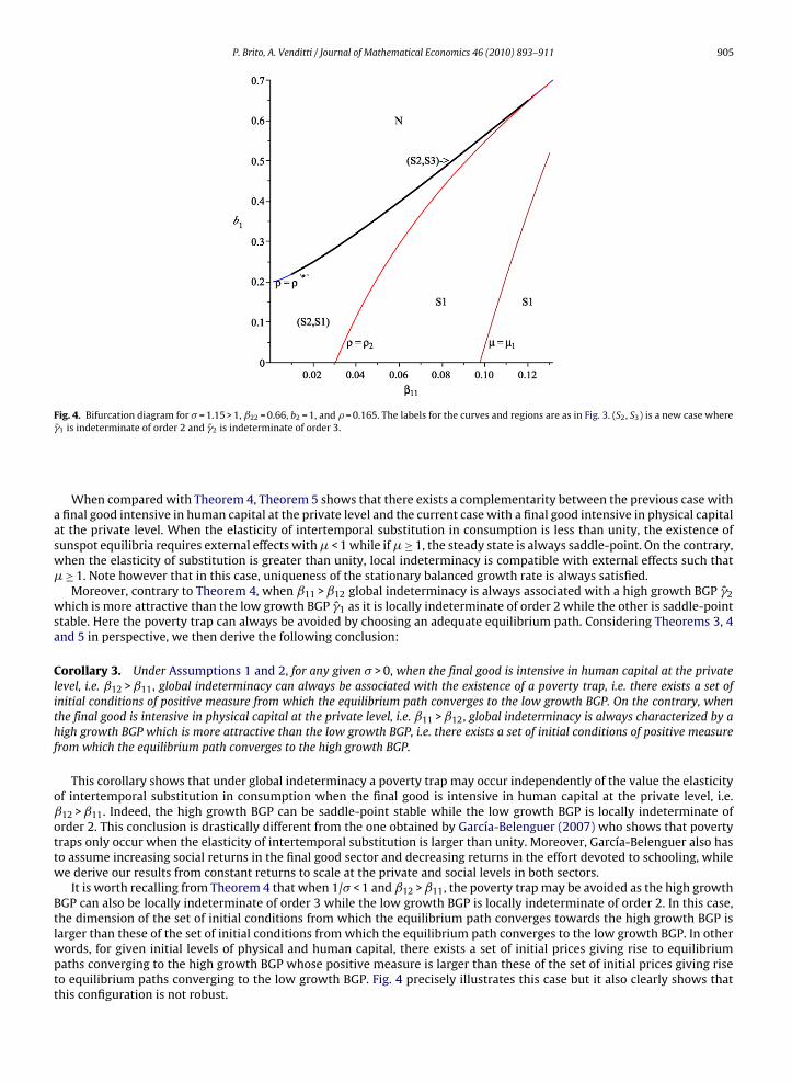
Theorem 4 shows that the local stability properties are sensitive with respect to the elasticity of intertemporal substitutionin consumption. When the elasticity is less than unity, i.e. 1/� < 1, external effects such that �≤ 1 imply local instability.Following Santos (2002) this means that there may not exist any equilibrium path.19 On the contrary, when externalities aresuch that �> 1, local and global indeterminacy can occur. An interesting new result is provided by case (1)-(ii)(a) in whichtwo distinct locally indeterminate stationary BGPs can co-exist. Such a globally indeterminate configuration has never beenillustrated previously. Moreover, and contrary to the configuration (1)-(i) in Theorem 3, the high growth BGP �2 can be moreattractive than the low growth BGP �1 as it can be locally indeterminate of order 3 while the other is locally indeterminateof order 2. In this case, the poverty trap can be avoided by choosing an adequate equilibrium path. Note however that thehigh growth BGP �2 can also be saddle-point stable while the low growth BGP �1 is locally indeterminate of order 2. In sucha case the poverty trap cannot be avoided. These configurations are illustrated in Fig. 4.20

When the elasticity of intertemporal substitution is on the contrary greater than unity, i.e. 1/� > 1, local and globalindeterminacy are compatible with both�≤ 1 and�> 1. However, when global indeterminay arises, one stationary balancedgrowth path is necessarily saddle-point stable. Moreover, global indeterminacy is now intimately related to the existence ofa poverty trap as in the case of Theorem 3. When stable, the low growth BGP �1 is locally indeterminate while the high growthBGP �2 is saddle-point stable. Theorems 3 and 4 then show that when ˇ12 <ˇ11, a poverty trap may occur independently ofthe value of the elasticity of intertemporal substitution in consumption 1/�.

We consider finally the configuration in which the final good is intensive in physical capital at the private level.

Theorem 5. Under Assumptions 1 and 2, let ˇ11 >ˇ12, and consider the bounds �1, �2 as defined by (22). Then the followingcases hold:

(1) Assume first that � > 1.(i) Let �≤�1 and � < �∗

2. (r, �) is locally indeterminate of order 2 if and only if D(r) − S(r)T(r)> 0.(ii) Let �∈ (�1, 1).(a) When �∈ (�∗

2, �∗), the steady states (r1, �1) and (r2, �2) are such that �2 > �1 and (r1, �1) is saddle-point stable, while

(r2, �2) is locally indeterminate of order 2 if and only if D(r2) − S(r2)T(r2)> 0.(b) When � ≤ �∗

2, (r, �) is locally indeterminate of order 2 if and only if D(r) − S(r)T(r)> 0.(iii) If �≥ 1 and � < �∗

2, (r, �) is saddle-point stable.(2) Assume now that � < 1.(i) If �< 1, any steady state is locally determinate.(ii) Let �≥ 1 and �∈ (�∗

1, �∗2). (r, �) is locally indeterminate of order 3 if and only if b2 > b1, T(r)< 0 and D(r) − S(r)T(r)> 0.


18 When b2 > b1 and T(r2)< 0, crossing the frontier D(r2) − S(r2)T(r2) = 0 implies the generic existence of a Hopf bifurcation and periodic cycles.19 There is a BGP only if (k1(0), k2(0)) belong to a particular one-dimensional manifold.20 The consideration of a large value for b1 is necessary to get the case (S2, S3). However, the existence of local and global indeterminacy with (S2, S1) can

be obtained with much lower values for b1.


Fig. 4. Bifurcation diagram for � = 1.15 > 1, ˇ22 = 0.66, b2 = 1, and � = 0.165. The labels for the curves and regions are as in Fig. 3. (S2, S3) is a new case where�1 is indeterminate of order 2 and �2 is indeterminate of order 3.

When compared with Theorem 4, Theorem 5 shows that there exists a complementarity between the previous case witha final good intensive in human capital at the private level and the current case with a final good intensive in physical capitalat the private level. When the elasticity of intertemporal substitution in consumption is less than unity, the existence ofsunspot equilibria requires external effects with�< 1 while if�≥ 1, the steady state is always saddle-point. On the contrary,when the elasticity of substitution is greater than unity, local indeterminacy is compatible with external effects such that�≥ 1. Note however that in this case, uniqueness of the stationary balanced growth rate is always satisfied.

Moreover, contrary to Theorem 4, when ˇ11 >ˇ12 global indeterminacy is always associated with a high growth BGP �2which is more attractive than the low growth BGP �1 as it is locally indeterminate of order 2 while the other is saddle-pointstable. Here the poverty trap can always be avoided by choosing an adequate equilibrium path. Considering Theorems 3, 4and 5 in perspective, we then derive the following conclusion:

Corollary 3. Under Assumptions 1 and 2, for any given � > 0, when the final good is intensive in human capital at the privatelevel, i.e. ˇ12 >ˇ11, global indeterminacy can always be associated with the existence of a poverty trap, i.e. there exists a set ofinitial conditions of positive measure from which the equilibrium path converges to the low growth BGP. On the contrary, whenthe final good is intensive in physical capital at the private level, i.e. ˇ11 >ˇ12, global indeterminacy is always characterized by ahigh growth BGP which is more attractive than the low growth BGP, i.e. there exists a set of initial conditions of positive measurefrom which the equilibrium path converges to the high growth BGP.

This corollary shows that under global indeterminacy a poverty trap may occur independently of the value the elasticityof intertemporal substitution in consumption when the final good is intensive in human capital at the private level, i.e.ˇ12 >ˇ11. Indeed, the high growth BGP can be saddle-point stable while the low growth BGP is locally indeterminate oforder 2. This conclusion is drastically different from the one obtained by García-Belenguer (2007) who shows that povertytraps only occur when the elasticity of intertemporal substitution is larger than unity. Moreover, García-Belenguer also hasto assume increasing social returns in the final good sector and decreasing returns in the effort devoted to schooling, whilewe derive our results from constant returns to scale at the private and social levels in both sectors.

It is worth recalling from Theorem 4 that when 1/� < 1 and ˇ12 >ˇ11, the poverty trap may be avoided as the high growthBGP can also be locally indeterminate of order 3 while the low growth BGP is locally indeterminate of order 2. In this case,the dimension of the set of initial conditions from which the equilibrium path converges towards the high growth BGP islarger than these of the set of initial conditions from which the equilibrium path converges to the low growth BGP. In otherwords, for given initial levels of physical and human capital, there exists a set of initial prices giving rise to equilibriumpaths converging to the high growth BGP whose positive measure is larger than these of the set of initial prices giving riseto equilibrium paths converging to the low growth BGP. Fig. 4 precisely illustrates this case but it also clearly shows thatthis configuration is not robust.


5. Concluding comments

We have studied the dynamics of a two-sector endogenous growth model with physical and human capital accumulationand economy-wide external effects in the production function of both sectors. Local and global indeterminacy have beendiscussed through the existence of multiple stationary balanced growth paths and through the local stability analysis ofeach long run position.

We have shown that two stationary balanced growth paths easily arise for a large set of parameters configurationswhich includes both signs for the capital intensity difference at the private level and values of the elasticity of intertemporalsubstitution in consumption lower or larger than unity. We have also proved that for a given stationary solution, two kindsof local indeterminacy can occur: a local indeterminacy of order 2 in which the stable manifold has dimension 2, and alocal indeterminacy of order 3 in which the stable manifold has dimension 3. This last case is particularly interesting aswe prove that in a configuration with two stationary solutions, one can be locally indeterminate of order 2 while the otheris locally indeterminate of order 3. This type of generalized local and global indeterminacy has never been illustrated inthe literature. Moreover, we have shown that local indeterminacy can be obtained independently of the sign of the capitalintensity difference at the private level and the value of the elasticity of intertemporal substitution in consumption. Fromthis point of view, we show that in our model, local and global indeterminacy are more robust properties than in most ofthe models considered in the literature.

Finally, we have discussed our main conclusions in terms of their implications for development economics. We haveproved that for any value of the elasticity of intertemporal substitution in consumption, global indeterminacy is alwaysassociated with the existence of a poverty trap when the final good is intensive in human capital at the private level.

Appendix A.

A.1. Proof of Lemma 1

From (5), we have

Kij/Yj ≡ aij = Pjˇij/RiWe call aij the input coefficient from the private viewpoint. Denoting A = [aij], Y = (Y1, Y2)′ and K = (K1, K2)′, it follows from (5)to (6) that AY = K. Moreover, denoting

P =(P1 00 P2

)and R =

(R1 00 R2

)

we have A = R−1BP. It follows from the constant returns to scale property of the individual technologies that the final goodis intensive in physical (human) capital at the private level, i.e. a11/a21 >(< )a12/a22, if and only if ˇ11 −ˇ12 >(< )0. Moreoverunder Assumption 1, A is invertible and

Y = A−1K ≡(˛11 ˛12

˛21 ˛22

)K =

⎛⎜⎝ R1

11

P1R2 12

P1

R1 21

P2R2 22

P2

⎞⎟⎠(K1

K2

)(24)

From this we get the optimal private allocations

Kij = ˇijRi

( j1R1K1 + j2R2K2

), for i, j = 1,2

which are linear functions of the total private amounts of the two capital stocks. The result follows from using again (5) andthe fact that the private returns to scale are constant.


Let k = k1/k2 = K1/K2. Proposition 1 and Eqs. (10)–(13) give

� =[(ˇ∗

1/ˇ∗2)kb1−b2

]1/(ˇ12+ˇ21)(25)

Substituting this into Eq. (11) gives

r =[(ˇ∗

1)ˇ12 (ˇ∗2)ˇ21kˇ12b1+ˇ21b2

]1/(ˇ12+ˇ21)(26)

Moreover, after solving Eqs. (14) and (15) we get:

�ˇ21r = �

k

[(ˇ11(� − 1) + ˇ12)r + �(ˇ11 − ˇ12)

](27)


Considering (25) and (26), we derive

�

k=[(ˇ∗

1)ˇ12+b2 (ˇ∗2)ˇ21−b1 r−(ˇ12+ˇ21+b2−b1)

]1/(ˇ12b1+ˇ21b2).

Substituting this into (27) finally gives the result.

A.3. Proof of Theorem 1

Note first that F(r) is monotone increasing (decreasing) if and only if �> 0 (�< 0) and concave (convex) if and only if�∈ (0, 1) (�∈(− ∞ , 0) ∪ (1, + ∞ )). Moreover

� > 0 ⇔ ˇ12(1 + b1) + ˇ21(1 + b2)> b1 − b2 (28)

� > 1 ⇔ ˇ12 + ˇ21 > b1 − b2 (29)

When ˇ11 <ˇ12, G(r) is monotone increasing for any value of � > 0. On the contrary, denoting � = (ˇ11 − ˇ12)/ˇ11, whenˇ11 >ˇ12, G(r) is monotone increasing (decreasing) if and only if� > � (� ∈ (0, �)). Our strategy for studying the existence andmultiplicity of stationary BGPs is based on the properties of these two functions (see Table 1 for some graphical illustrations).Indeed if F(r) and G(r) have opposite slopes, there exists at most one stationary balanced growth rate. Some boundaryconditions can then guarantee existence. On the contrary, if both F(r) and G(r) have positive or negative slopes, we can finda tangency point between these two functions by solving simultaneously F(r) = G(r) and F′(r) = G′(r) with respect to r and�. This gives the following values:

r∗ =(ˇ11(� − 1) + ˇ12

��ˇ21 ˜

)1/(�−1)

, �∗ = (1 −�)[ˇ11(� − 1) + ˇ12]�(ˇ11 − ˇ12)

r∗ (30)

When � =�∗, r∗ is a tangency point between F(r) and G(r). Additional conditions on the parameters of the model that willbe necessary to get admissible values for r∗ and �∗ are straightforward from (20), namely � > � ≡ (ˇ11 − ˇ12)/ˇ11 ∈ (0,1),and:

(i) ˇ12 >ˇ11 and �∈(− ∞ , 0) ∪ (1, + ∞ ), or(ii) ˇ12 <ˇ11 and �∈ (0, 1).

When such an admissible tangency point exists, we define the corresponding growth rate as �∗ = (r∗ −�∗)/�. UnderAssumption 2, as � = (r −�)/�, the long run real rate of return should verify the condition �− (1 −�)r > 0. Moreover, since� > 0 we need to have r >�. It follows that r is defined over (�, + ∞ ) when � ≥ 1 while it is defined over (�, �/(1 −�)) when� ∈ (0, 1). These restrictions allow to define lower and upper bounds for the discount factor�. Indeed, solving simultaneouslyF(�/(1 − �)) = G(�/(1 − �)) and F(�) = G(�) with respect to � gives respectively

�1 = (1 − �)

(ˇ21

ˇ12

˜)1/(1−�)

, �2 =(ˇ21

ˇ11

˜)1/(1−�)

(31)

Note that �1 can be negative and the difference �2 −�1 can be positive or negative.From all these results, we now study the existence and uniqueness of a stationary balanced growth rate. Let us define

�1 = ˇ11(� − 1) + ˇ12

�ˇ11, �2 = ˇ11(� − 1) + ˇ12

�ˇ12(32)

(i) When ˇ11 <ˇ12, we get �1 > 1 and �2 ∈ (0, 1) when � ≥ 1, while �2 > 1 when � ∈ (0, 1). Moreover we have �1 >�2. Forany value of � > 0, G(r) is monotone increasing. Multiple solutions for Eq. (18) can only arise if F(r) is increasing and convex,i.e. when�> 1. In this case, when � =�∗, r∗ is a tangency point between F(r) and G(r). Therefore multiplicity will hold in thefollowing cases:(a) If � ≥ 1, we need to have r∗ >�∗, i.e. �∈ (1, �1). Recall that with �> 1, limr→+∞F′(r) = +∞ and thus limr→+∞[F(r) −G(r)]> 0. Since ˇ11 <ˇ12, we have lim�→+∞G(0) = −∞. Then, when � >�∗, F(r) lies above G(r) and no intersection occurs.When � =�∗, the tangency point r∗ is the unique solution of Eq. (18). When � <�∗, two solutions can occur provided � isnot too small. Indeed from the restriction r >� we have to consider the solution of F(�) = G(�) with respect to �. We get�2 as defined by (21) and a condition for multiplicity is �∈ (�2, �∗).(b) If � ∈ (0, 1), we need to have r∗ >�∗ and r∗ <�∗/(1 −�), i.e. �∈ (�2, �1). When � >�∗, F(r) lies above G(r) and no inter-section occurs. When � =�∗, the tangency point r∗ is the unique solution of Eq. (18). When � <�∗, from the restrictionsr >� and r <�/(1 −�), we have to consider �2 and the solution of F(�/(1 − �)) = G(�/(1 − �)) with respect to �. We get�1 as defined by (21). Now we define �∗

1 = max{0,min{�1, �2}} and �∗2 = max{�1, �2}. Two solutions will occur provided

�∈ (�∗2, �

∗). Result (i) is obtained from the restriction �∈ (�2, �1).


When ˇ11 >ˇ12, G(r) is monotone increasing if � ≥ (ˇ11 − ˇ12)/ˇ11 ≡ � and monotone decreasing if � < �. Multiplesolutions for Eq. (18) can only arise if F(r) and G(r) are both increasing or decreasing, and the tangency point is into thedomain of definition.

(ii) Consider first the case� ≥ � in which�1 ∈ (0, 1),�2 ∈ (0, + ∞ ) and�2 >�1. Multiplicity then requiresF(r) to be increasingand concave, i.e. �∈ (0, 1).(a) If � ≥ 1, we need to have r∗ >�∗, i.e. �∈ (�1, min {1, �2}). As in case (i)-(a), multiplicity is obtained under �∈ (�∗

2, �∗).

(b) If� ∈ [�,1), we need to have r∗ >�∗ and r∗ <�∗/(1 −�), i.e.�∈ (�1, min {1,�2}). As in case (i)-(b), multiplicity is obtainedunder �∈ (�∗

2, �∗).

Result (ii) is obtained from the restriction �∈ (�1, min {1, �2}).(iii) Consider finally the case � ∈ (0, �] in which �2 <�1 < 0 and the tangency point (r∗, �∗) does not exist. Multiplicity thenrequires F(r) to be decreasing and convex, i.e. �< 0. Since ˇ11 >ˇ12, we have lim�→+∞G(0) = +∞. Then, two solutions canoccur provided � is not too big. From the restrictions r >� and r <�/(1 −�), we have indeed to consider �1 and �2 as definedby (21). Two solutions will then occur provided �∈ (0, �∗

1).

A.4. Proof of Corollary 1

(i) Assume that b1 = b2 = b > 0. We derive from (29) that�> 1. It follows therefore from Theorem 1 that two stationary BGPsexist if ˇ11 <ˇ12, �∈ (�2, �1) ⊂ (1, + ∞ ) and �∈ (�∗

2, �∗).

(ii) Assume that b1 = 0 and b2 ∈ (0, 1). We derive from (29) that �> 1 and the same conclusions as in case (i) hold.

A.5. Proof of Corollary 2

Assume that b1 ∈ (0, 1) and b2 = 0. When ˇ12 > 0 we derive �= (ˇ12 −ˇ11 + 1 − b1ˇ22)/ˇ12b1 which can be positive ornegative depending on the values of the various parameters. Multiple stationary BGP’s can then arise if one of the conditionsgiven in Theorem 1 holds. On the contrary, when ˇ12 = 0, we derive immediately from Eq. (11) that the stationary rental rateof capital is r = 1. The associated stationary BGP is then � = (1 −�)/� and the result follows.


(i) Consider the case � ≥ 1. Recall that the domain of definition of r is (�, + ∞ ). For any value of � ≥ 1, G(r) is monotoneincreasing. We will discuss the different configurations depending on the sign of ˇ11 −ˇ12. Note that for any sign of thiscapital intensity difference, F(r) is non-increasing when �≤ 0. It follows that if �≤ 0, there exists a unique solution for Eq.(18) provided F(�)> G(�), i.e. � < �∗

2 = �2, with �2 given by (21).(a) Let ˇ11 <ˇ12. When �∈ (0, 1], F(r) is increasing and concave with limr→+∞F′(r) = 0. It follows that limr→+∞[F(r) −G(r)]< 0. Therefore if�≤ 1, there exists a unique solution for Eq. (18) provided F(�)> G(�), i.e. � < �∗

2. If on the contrary�> 1, r∗ is a tangency point betweenF(r) andG(r) when� =�∗. The interiority condition is r∗ >�∗, i.e.�<�1. If this inequalityis satisfied, we know from Theorem 1 that existence and uniqueness will hold as soon as � < �∗

2. If the interiority conditiondoes not hold, i.e.�≥�1, F(r) is increasing and convex with limr→+∞[F(r) − G(r)]> 0. Then there exists a unique solutionfor Eq. (18) provided F(�)< G(�). Since �> 1, this gives again the condition � < �∗

2.(b) Let ˇ11 >ˇ12. When �∈ (0, 1), r∗ is a tangency point between F(r) and G(r) when � =�∗ provided the interioritycondition r∗ >�∗ is satisfied, i.e. 1 >�>�1. In this case, Theorem 1 implies that existence and uniqueness will hold assoon as � < �∗

2. If the interiority condition does not hold, i.e. �≤�1, F(r) is concave with limr→+∞[F(r) − G(r)]< 0.Existence and uniqueness hold when F(�)> G(�), i.e. � < �∗

2. Finally, if �> 1 F(r) is convex with limr→+∞[F(r) −G(r)]> 0. There exists a unique stationary balanced growth rate if F(�)< G(�). Since �≥ 1, this gives again� < �∗

2.(ii) We have now to consider the case � ∈ (0, 1). Recall that the domain of definition of r is (�, �/(1 −�)). If ˇ11 <ˇ12,G(r) is monotone increasing for any � ∈ (0, 1). The same results as in the previous configurations (i)-(a) hold exceptthe fact that since r ∈ (�, �/(1 −�)), existence and uniqueness require F(�)> G(�) and F(�/(1 − �))< G(�/(1 − �)). Therestriction on the discount rate then becomes �∈ (�∗

1, �∗2). If on the contrary ˇ11 >ˇ12, G(r) is monotone increasing if

� ≥ � and monotone decreasing if � < �. When � ≥ �, the same results as in the previous configurations (i)-(b) holdwith �∈ (�∗

1, �∗2). We need therefore to study the case � ∈ (0, �) where the tangency point (r∗, �∗) does not exist. When

�≤ 0, F(r) is also non-increasing. Then, if �∈ (�2, �1), Theorem 1 implies that existence and uniqueness will hold assoon as �∈ (�∗

1, �∗2). If on the contrary � /∈ (�2, �1), we obtain the following conditions: if �≤�2, existence and unique-

ness hold when F(�)< G(�) and F(�/(1 − �))> G(�/(1 − �)). Since �< 0 this gives again �∈ (�∗1, �

∗2). On the contrary,

if 0 >�≥�1, existence and uniqueness hold when F(�)> G(�) and F(�/(1 − �))< G(�/(1 − �)), i.e. �∈ (�∗1, �

∗2). Finally, if

�≥ 0 F(r) is non-decreasing and existence and uniqueness will hold when F(�)< G(�) and F(�/(1 − �))> G(�/(1 − �)), i.e.�∈ (�∗

1, �∗2).


A.7. Proof of Proposition 2

Let k = k1/k2. Linearising the dynamical system (12)–(15) around a stationary BGP gives the Jacobian matrix

J =(

J11 J12

Ja21 + Jb21 + Jc21 J22

)(33)

with

J11 =(r − ˛11 −˛21−˛12 r − ˛22

), J12 = −r

⎛⎝ �11

p1

k1�21p1

k2

�12p2

k1�22p2

k2

⎞⎠ ,

Ja21 = 1r

⎛⎜⎝

k1

p1˛2

11 + k2

p2˛2

12k1

p1˛11˛21 + k2

p2˛12˛22

k1

p1˛11˛21 + k2

p2˛12˛22

k1

p1˛2

21 + k2

p2˛2

22

⎞⎟⎠

Jb21 = −

⎛⎜⎝k1

p1˛11 + k2

p1˛12 0

0k1

p2˛21 + k2

p2˛22

⎞⎟⎠ , Jc21 =

⎛⎜⎝ 1�p

−1 + ��

1 0

0 0

⎞⎟⎠

and

J22 =(˛11�11 + ˛12�12k−1 + ˛11 − � ˛12�22 + ˛11�21k + ˛12

˛21�11 + ˛22�12k−1 + ˛21 ˛22�22 + ˛21�21k + ˛22 − �

)

For i = 0, 1, 2, 3, let �i(r) be the sum of the principal minors of order 4 − i of the Jacobian matrix (33) evaluated at some steadystate r. Some tedious computations available upon request allow to simplify the expressions of each �i(r) and to provide theresults of the Proposition with T(r) = �1(r), S(r) = �2(r), D(r) = �3(r) and(r) = �4(r).


The tangency point r∗ and the corresponding value �∗ are defined as the solutions of the following system

F(r∗) = G(r∗), F′(r∗) = G′(r∗)

Since G(r) is linear and F(r) is parabolic we can write

F(r∗) = rG′(r∗) + �(ˇ11 − ˇ12), F′(r∗) = �F(r∗)r∗

= G′(r∗)

It follows that�G(r∗) = r∗G′(r∗). Consider now the term between brackets into the expression of D(r) given in Proposition 2.We have

G(r∗)(�− 1) + �(ˇ11 − ˇ12) = rG′(r∗) − G(r∗) + �(ˇ11 − ˇ12) = 0

Moreover, for any r /= r∗, we have

G(r)(�− 1) + �(ˇ11 − ˇ12) = r(F′(r) − G′(r)

)Under Assumptions 1 and 2 [r − �(ˇ11 − ˇ12)]> 0 and the result follows.


Let � = 1.

(1) We start by the case ˇ11 <ˇ12. Theorem 2 shows that when �≤ 1 and � <�2, the unique steady state r is such thatF′(r) − G′(r)< 0 while r is such that F′(r) − G′(r)> 0 when �≥ˇ12/ˇ11 and � <�2. Consider now Theorem 1 with �∈ (1,ˇ12/ˇ11) and � <�∗. When �∈ (�2, �∗), denote the two steady states r1, r2 such that r1 < r2. We then have F′(r1) − G′(r1)< 0and F′(r2) − G′(r2)> 0. When �∈ (0, �2], there is one unique steady state r2 such that F′(r) − G′(r2)> 0. We then prove thethree different cases:


(i) When �≤ 1 and � <�2, D(r)> 0. Moreover from Eq. (29) we necessarily have b2 − b1 < 0. It follows that T(r)> 0 andthus T(r) + ı > 0 so that the steady state is locally unstable.(ii) When �∈ (1, ˇ12/ˇ11), we have D(r1)> 0 as long as �∈ (�2, �∗) and local indeterminacy of order 2 holds if and only ifT(r1) + ı1 < 0. On the contrary, for any �∈ (0, �∗), D(r2)< 0 and (r2, �2) is saddle-point stable.(iii) Finally, when �≥ˇ12/ˇ11 and � <�2, D(r)< 0 and saddle-point stability holds.

(2) Consider now the case ˇ11 >ˇ12. From Theorem 2 and Table 1, we derive that when �≤ˇ12/ˇ11 and � <�2, the uniquesteady state r is such that F′(r) − G′(r)< 0 while r is such that F′(r) − G′(r)> 0 when �≥ 1 and � <�2. On the contraryTheorem 1 shows that when �∈ (ˇ12/ˇ11, 1) and �∈ (�2, �∗), the two steady states r1, r2 are such that F′(r1) − G′(r1)< 0and F′(r2) − G′(r2)> 0. When �∈ (0, �2], the unique steady state r2 is such that F′(r2) − G′(r2)> 0. We then prove the threedifferent cases:(i) When �≤ˇ12/ˇ11 and � <�2, D(r)> 0 and from Eq. (29) we necessarily have b2 − b1 < 0. It follows that T(r)> 0 andthus T(r) + ı > 0 so that the steady state is locally unstable.(ii) When �∈ (ˇ12/ˇ11, 1), we have D(r1)> 0 as long as �∈ (�2, �∗) and for any �∈ (0, �∗), D(r2)< 0. Since b2 − b1 < 0, itfollows that (r1, �1) is locally unstable while (r2, �2) is saddle-point stable.(iii) Finally, when �≥ 1 and � <�2, D(r)< 0 and saddle-point stability holds.


We will use the following Proposition from Barinci and Drugeon (1999) which provides a set of useful criteria for assessingthe local determinacy/indeterminacy of intertemporal equilibria in economies described by 3-dimensional continuous-timedynamical systems.

Proposition 3. Consider an economy locally described by a characteristic polynomial of degree 3 such that

g() = 3 − T2 + S− D

The dimension of the local stable manifold is as follows:

(i) for T< 0, if D< 0 and D> ST, there are three eigenvalues with negative real parts;(ii) for T< 0 and D> 0 or for T> 0, D> 0 and D> ST, there are two eigenvalues with negative real parts;

(iii) for T< 0, if D< 0 and D< ST or, for T> 0, if D< 0, there is one eigenvalue with negative real part;(iv) for T> 0, if D> 0 and D< ST, there is no eigenvalue with negative real part.

We now prove Theorem 4. Let ˇ11 <ˇ12 and recall that

D(r) − S(r)T(r) = −(ı+ T(r))D(r) − T(r)[ı(ı+ T(r)) + Y(r)

](34)

Depending on the value of � and �, the proof is derived from Theorems 1 and 2, Lemma 3, Propositions 2 and 3 and Eq.(31). We will only give a detailed argument for case 1 of Theorem 4. Consider the bounds �1, �2 as defined by (29).

(1) Assume first that � > 1. From Proposition 2 we derive Y(r)> 0.(i) If �≤ 1 and � < �∗

2, then D(r)> 0. Moreover, we get from Eq. (29) that b2 − b1 is necessarily negative so that T(r)> 0.It follows that T(r)> 0, S(r)> 0 and, from Eq. (34), D(r) − S(r)T(r)< 0. Proposition 3 implies that (r, �) is locally unstable.(ii) Let �∈ (1, �1) and consider Theorem 1 and Lemma 3. When �∈ (�∗

2, �∗), the steady states (r1, �1) and (r2, �2) are such

that D(r1)> 0 and D(r2)< 0. Proposition 3 implies that (r1, �1) is locally indeterminate of order 2 if T(r1)< 0, or T(r1)> 0andD(r1) − S(r1)T(r1)> 0, while (r2, �2) is locally indeterminate of order 3 if and only ifT(r2)< 0 andD(r2) − S(r2)T(r2)> 0.When � ≤ �∗

2, the unique remaining steady state (r, �) is such that D(r)< 0. The result follows from Proposition 3.(iii) If �≥�1 and � < �∗

2, then D(r)< 0. The result follows from Proposition 3.(2) Assume now that � < 1. From Proposition 2 we derive Y(r)< 0.(i) If �≤ 1 and �∈ (�∗

1, �∗2), we have T(r)> 0 and D(r)> 0.

(ii) If �∈ (1, �2) and �∈ (�∗1, �

∗2), we have D(r)> 0.

(iii) Let�∈ (�2,�1). When �∈ (�∗2, �

∗), the steady states (r1, �1) and (r2, �2) are such that: D(r1)> 0 and D(r2)< 0. When�∈ (�∗

1, �∗2], consider the bounds �1 and �2 defined by Eq. (21). The unique remaining steady state (r, �) is such that

D(r)< 0 or D(r)> 0 depending on whether the difference �2 −�1 is positive or negative. The result follows from the factthat �2 −�1 > 0 if and only if � > 1 − (ˇ12/ˇ11)1/(1−�).(iv) If �≥�1 and �∈ (�∗

1, �∗2), we have D(r)< 0.


Let ˇ11 >ˇ12. We proceed as in the proof of Theorem 4. Depending on the value of � and �, the results are derived fromTheorems 1 and 2, Lemma 3, Propositions 2 and 3 and Eq. (34).


(1) Assume first that � > 1. From Proposition 2 we derive Y(r)< 0.(i) If �≤�1 and � < �∗

2, we have T(r)> 0 and D(r)> 0.(ii) If �∈ (�1, 1), we have T(r)> 0. When �∈ (�∗

2, �∗), the steady states (r1, �1) and (r2, �2) are such that: D(r1)< 0 and

D(r2)> 0. When � ≤ �∗2, the unique remaining steady state (r, �) is such that D(r)> 0.

(iii) If �≥ 1 and � < �∗2, we have D(r)< 0.

(2) Assume now that � < 1. From Proposition 2 we derive Y(r)> 0.(i) If �< 1, we necessarily have T(r)> 0. Therefore any steady state will be either saddle-point stable if D(r)< 0 or locallyunstable if D(r)> 0 since in this case we have S(r)> 0 and D(r) − S(r)T(r)< 0.(ii) If �≥ 1 and �∈ (�∗

1, �∗2), we have D(r)< 0.

References

d’Autume, A., Michel, P., 1992. The New Growth Theories. Part 1: Persistence, Hysteresis and Multiple Equilibria. DP 92.20 (in French), University of Paris 1.Azariadis, C., Stachurski, J., 2005. Poverty traps. In: Aghion, P., Durlauf, S. (Eds.), Handbook of Economic Growth, vol. 1. North-Holland, Amsterdam, pp.

295–384.Barinci, J.P., Drugeon, J.P., 1999. Assessing Local Indeterminacy in Three-Dimensional Dynamical Systems: A Geometric Perspective, mimeo, EUREQua.Basu, S., Fernald, J., 1997. Returns to scale in US production: estimates and implications. Journal of Political Economy 105, 249–283.Ben-Gad, M., 2003. Fiscal policy and indeterminacy in models of endogenous growth. Journal of Economic Theory 108, 322–344.Benhabib, J., Meng, Q., Nishimura, K., 2000. Indeterminacy under constant returns in multisector economies. Econometrica 68, 1541–1548.Benhabib, J., Perli, R., 1994. Uniqueness and indeterminacy: transitional dynamics in a model of endogenous growth. Journal of Economic Theory 63,

113–142.Bloise, G., 2001. A geometric approach to sunspot equilibria. Journal of Economic Theory 101, 519–539.Bond, E., Wang, P., Yip, C., 1996. A general two-sector model of endogenous growth with human and physical capital: balanced growth and transitional

dynamics. Journal of Economic Theory 68, 149–173.Boucekkine, R., Martinez, B., Ruiz-Tamarit, R., 2008. A note on global dynamics and imbalance effects in the Lucas-Uzawa model. International Journal of

Economic Theory 4, 503–518.Boucekkine, R., Ruiz-Tamarit, R., 2008. Special functions for the study of economic dynamics: the case of the Lucas-Uzawa model. Journal of Mathematical

Economics 44, 33–54.Caballe, J., Santos, M., 1993. On endogenous growth with physical and human capital. Journal of Political Economy 101, 1042–1068.Chamley, C., 1993. Externalities and dynamics in models of learning-by-doing. International Economic Review 34, 583–609.Drugeon, J.P., 2008. On intersectoral asymmetries in factors substitutability, “Equilibrium Production Possibility Frontiers” and the emergence of indeter-

minacies. Journal of Mathematical Economics 44, 277–315.Drugeon, J.P., Poulsen, O., Venditti, A., 2003. On intersectoral allocations, factors substitutability and multiple long-run growth paths. Economic Theory 21,

175–183.García-Belenguer, F., 2007. Stability, global dynamics and Markov equilibrium in models of endogenous economic growth. Journal of Economic Theory 136,

392–416.Ladrón-de-Guevara, A., Ortigueira, S., Santos, M., 1997. Equilibrium dynamics in two sector models of endogenous growth. Journal of Economic Dynamics

and Control 21, 115–143.Ladrón-de-Guevara, A., Ortigueira, S., Santos, M., 1999. A two sector model of endogenous growth with leisure. Review of Economic Studies 66, 609–631.Leonard, D., Van Long, N., 1992. Optimal Control Theory and Static Maximization in Economics. Cambridge University Press.Lucas, R., 1988. On the mechanics of economic development. Journal of Monetary Economics 22, 3–42.Mattana, P., Nishimura, K., Shigoka, T., 2009. Homoclinic bifurcation and global indeterminacy of equilibrium in a two-sector endogenous growth model.

International Journal of Economic Theory 5, 25–47.Mino, K., 2001. Indeterminacy and endogenous growth with social constant returns. Journal of Economic Theory 97, 203–222.Mitra, T., 1998. On equilibrium dynamics under externalities in a model of economic development. Japanese Economic Review 49, 85–107.Mulligan, C., Sala-i-Martin, X., 1993. Transitional dynamics in two sector models of endogenous growth. Quarterly Journal of Economics 103, 739–773.Nishimura, K., Takahashi, H., Venditti, A., 2009. Global externalities, endogenous growth and sunspot fluctuations. Advanced Studies in Pure Mathematics

53, 227–238.Nishimura, K., Venditti, A., 2004. Indeterminacy and the role of factor substitutability. Macroeconomic Dynamics 8, 436–465.Raurich, X., 2001. Indeterminacy and government spending in a two-sector model of endogenous growth. Review of Economic Dynamics 4, 210–229.Rebelo, S., 1991. Long-run policy analysis and long-run growth. Journal of Political Economy 99, 500–521.Romer, P., 1986. Increasing returns and long-run growth. Journal of Political Economy 94, 1002–1037.Santos, M., 2002. On non-existence of Markov equilibria in competitive-market economies. Journal of Economic Theory 105, 73–98.Woodford, M., 1986. Stationary Sunspot Equilibria: The Case of Small Fluctuations Around a Deterministic Steady Sate. mimeo, University of Chicago.Xie, D., 1994. Divergence in economic performance: transitional dynamics with multiple equilibria. Journal of Economic Theory 63, 97–112.

local and global indeterminacy in two-sector models of endogenous growth

Documents