local and global asymptotic inference …
TRANSCRIPT

arX
iv:1
212.
6788
v3 [
mat
h.ST
] 2
6 N
ov 2
013
The Annals of Statistics
2013, Vol. 41, No. 5, 2608–2638DOI: 10.1214/13-AOS1164c© Institute of Mathematical Statistics, 2013
LOCAL AND GLOBAL ASYMPTOTIC INFERENCE
IN SMOOTHING SPLINE MODELS
By Zuofeng Shang and Guang Cheng1
University of Notre Dame and Purdue University
This article studies local and global inference for smoothing splineestimation in a unified asymptotic framework. We first introduce anew technical tool called functional Bahadur representation, whichsignificantly generalizes the traditional Bahadur representation inparametric models, that is, Bahadur [Ann. Inst. Statist. Math. 37
(1966) 577–580]. Equipped with this tool, we develop four inter-connected procedures for inference: (i) pointwise confidence interval;(ii) local likelihood ratio testing; (iii) simultaneous confidence band;(iv) global likelihood ratio testing. In particular, our confidence in-tervals are proved to be asymptotically valid at any point in thesupport, and they are shorter on average than the Bayesian confi-dence intervals proposed by Wahba [J. R. Stat. Soc. Ser. B Stat.Methodol. 45 (1983) 133–150] and Nychka [J. Amer. Statist. Assoc.83 (1988) 1134–1143]. We also discuss a version of the Wilks phe-nomenon arising from local/global likelihood ratio testing. It is alsoworth noting that our simultaneous confidence bands are the firstones applicable to general quasi-likelihood models. Furthermore, is-sues relating to optimality and efficiency are carefully addressed. Asa by-product, we discover a surprising relationship between periodicand nonperiodic smoothing splines in terms of inference.
1. Introduction. As a flexible modeling tool, smoothing splines provide ageneral framework for statistical analysis in a variety of fields; see [13, 41, 42].The asymptotic studies on smoothing splines in the literature focus primar-ily on the estimation performance, and in particular the global convergence.However, in practice it is often of great interest to conduct asymptotic in-ference on the unknown functions. The procedures for inference developedin this article, together with their rigorously derived asymptotic properties,fill this long-standing gap in the smoothing spline literature.
Received August 2013.1Sponsored by NSF Grant DMS-09-06497 and CAREER Award DMS-11-51692.AMS 2000 subject classifications. Primary 62G20, 62F25; secondary 62F15, 62F12.Key words and phrases. Asymptotic normality, functional Bahadur representation, lo-
cal/global likelihood ratio test, simultaneous confidence band, smoothing spline.
This is an electronic reprint of the original article published by theInstitute of Mathematical Statistics in The Annals of Statistics,2013, Vol. 41, No. 5, 2608–2638. This reprint differs from the original inpagination and typographic detail.
1

2 Z. SHANG AND G. CHENG
As an illustration, consider two popular nonparametric regression mod-els: (i) normal regression: Y | Z = z ∼N(g0(z), σ
2) for some unknown σ2 > 0;(ii) logistic regression: P (Y = 1 | Z = z) = exp(g0(z))/(1 + exp(g0(z))). Thefunction g0 is assumed to be smooth in both models. Our goal in this pa-per is to develop asymptotic theory for constructing pointwise confidenceintervals and simultaneous confidence bands for g0, testing on the value ofg0(z0) at any given point z0, and testing whether g0 satisfies certain globalproperties such as linearity. Pointwise confidence intervals and tests on alocal value are known as local inference. Simultaneous confidence bands andtests on a global property are known as global inference. To the best of ourknowledge, there has been little systematic and rigorous theoretical study ofasymptotic inference. This is partly because of the technical restrictions ofthe widely used equivalent kernel method. The functional Bahadur represen-tation (FBR) developed in this paper makes several important contributionsto this area. Our main contribution is a set of procedures for local and globalinference for a univariate smooth function in a general class of nonparamet-ric regression models that cover both the aforementioned cases. Moreover,we investigate issues relating to optimality and efficiency that have not beentreated in the existing smoothing spline literature.
The equivalent kernel has long been used as a standard tool for handlingthe asymptotic properties of smoothing spline estimators, but this methodis restricted to least square regression; see [26, 35]. Furthermore, the equiv-alent kernel only “approximates” the reproducing kernel function, and theapproximation formula becomes extremely complicated when the penaltyorder increases or the design points are nonuniform. To analyze the smooth-ing spline estimate in a more effective way, we employ empirical processtheory to develop a new technical tool, the functional Bahadur representa-tion, which directly handles the “exact” reproducing kernel, and makes itpossible to study asymptotic inference in a broader range of nonparametricmodels. An immediate consequence of the FBR is the asymptotic normalityof the smoothing spline estimate. This naturally leads to the constructionof pointwise asymptotic confidence intervals (CIs). The classical BayesianCIs in the literature [28, 40] are valid on average over the observed covari-ates. However, our CIs are proved to be theoretically valid at any point, andthey even have shorter lengths than the Bayesian CIs. We next introduce alikelihood ratio method for testing the local value of a regression function.It is shown that the null limiting distribution is a scaled Chi-square withone degree of freedom, and that the scaling constant converges to one as thesmoothness level of the regression function increases. Therefore, we havediscovered an interesting Wilks phenomenon (meaning that the asymptoticnull distribution is free of nuisance parameters) arising from the proposednonparametric local testing.

ASYMPTOTIC INFERENCE FOR SMOOTHING SPLINE 3
Procedures for global inference are also useful. Simultaneous confidencebands (SCBs) accurately depict the global behavior of the regression func-tion, and they have been extensively studied in the literature. However,most of the efforts were devoted to simple regression models with addi-tive Gaussian errors based on kernel or local polynomial estimates; see[5, 11, 17, 38, 44]. By incorporating the reproducing kernel Hilbert space(RKHS) theory into [2], we obtain an SCB applicable to general nonpara-metric regression models, and we demonstrate its theoretical validity basedon strong approximation techniques. To the best of our knowledge, this isthe first SCB ever developed for a general nonparametric regression model insmoothing spline settings. We further demonstrate that our SCB is optimalin the sense that the minimum width of the SCB achieves the lower boundestablished by [12]. Model assessment is another important aspect of globalinference. Fan et al. [9] used local polynomial estimates for testing non-parametric regression models, namely the generalized likelihood ratio test(GLRT). Based on smoothing spline estimates, we propose an alternativemethod called the penalized likelihood ratio test (PLRT), and we identifyits null limiting distribution as nearly Chi-square with diverging degreesof freedom. Therefore, the Wilks phenomenon holds for the global test aswell. More importantly, we show that the PLRT achieves the minimax rateof testing in the sense of [19]. In comparison, other smoothing-spline-basedtests such as the locally most powerful (LMP) test, the generalized cross val-idation (GCV) test and the generalized maximum likelihood ratio (GML)test (see [4, 6, 20, 23, 30, 41]) either lead to complicated null distributionswith nuisance parameters or are not known to be optimal.
As a by-product, we derive the asymptotic equivalence of the proposedprocedures based on periodic and nonperiodic smoothing splines under mildconditions; see Remark 5.2. In general, our findings reveal an intrinsic con-nection between the two rather different basis structures, which in turnfacilitates the implementation of inference.
Our paper is mainly devoted to theoretical studies. However, a few practi-cal issues are noteworthy. GCV is currently used for the empirical tuning ofthe smoothing parameter, and it is known to result in biased estimates if thetrue function is spatially inhomogeneous with peaks and troughs. Moreover,the penalty order is prespecified rather than data-driven. Future researchis needed to develop an efficient method for choosing a suitable smoothingparameter for bias reduction and an empirical method for quantifying thepenalty order through data. We also note that some of our asymptotic pro-cedures are not fully automatic since certain quantities need to be estimated;see Example 6.3. A large sample size may be necessary for the benefits ofour asymptotic methods to become apparent. Finally, we want to mentionthat extensions to more complicated models such as multivariate smooth-ing spline models and semiparametric models are conceptually feasible byapplying similar FBR techniques and likelihood-based approaches.

4 Z. SHANG AND G. CHENG
The rest of this paper is organized as follows. Section 2 introduces the ba-sic notation, the model assumptions, and some preliminary RKHS results.Section 3 presents the FBR and the local asymptotic results. In Sections 4and 5, several procedures for local and global inference together with theirtheoretical properties are formally discussed. In Section 6, we give three con-crete examples to illustrate our theory. Numerical studies are also providedfor both periodic and nonperiodic splines. The proofs are included in anonline supplementary document [33].
2. Preliminaries.
2.1. Notation and assumptions. Suppose that the data Ti = (Yi,Zi), i=1, . . . , n, are i.i.d. copies of T = (Y,Z), where Y ∈ Y ⊆ R is the responsevariable, Z ∈ I is the covariate variable and I = [0,1]. Consider a generalclass of nonparametric regression models under the primary assumption
µ0(Z)≡E(Y | Z) = F (g0(Z)),(2.1)
where g0(·) is some unknown smooth function and F (·) is a known linkfunction. This framework covers two subclasses of statistical interest. Thefirst subclass assumes that the data are modeled by yi | zi ∼ p(yi;µ0(zi)) fora conditional distribution p(y;µ0(z)) unknown up to µ0. Instead of assum-ing known distributions, the second subclass specifies the relation betweenthe conditional mean and variance as Var(Y | Z) = V(µ0(Z)), where V is aknown positive-valued function. The nonparametric estimation of g in thesecond situation uses the quasi-likelihood Q(y;µ) ≡
∫ µy (y − s)/V(s)ds as
an objective function (see [43]), where µ= F (g). Despite distinct modelingprinciples, the two subclasses have a large overlap since Q(y;µ) coincideswith log p(y;µ) under many common combinations of (F,V); see Table 2.1of [25].
From now on, we focus on a smooth criterion function ℓ(y;a) :Y ×R 7→R
that covers the above two cases, that is, ℓ(y;a) =Q(y;F (a)) or log p(y;F (a)).Throughout this paper, we define the functional parameter space H as themth-order Sobolev space:
Hm(I)≡ {g : I 7→R | g(j) is absolutely continuous
for j = 0,1, . . . ,m− 1 and g(m) ∈L2(I)},where m is assumed to be known and larger than 1/2. With some abuse ofnotation, H may also refer to the homogeneous subspace Hm
0 (I) of Hm(I).The space Hm
0 (I) is also known as the class of periodic functions such thata function g ∈ Hm
0 (I) has the additional restrictions g(j)(0) = g(j)(1) forj = 0,1, . . . ,m− 1. Let J(g, g) =
∫Ig(m)(z)g(m)(z)dz. Consider the penalized
ASYMPTOTIC INFERENCE FOR SMOOTHING SPLINE 5
nonparametric estimate gn,λ:
gn,λ = argmaxg∈H
ℓn,λ(g)
(2.2)
= argmaxg∈H
{1
n
n∑
i=1
ℓ(Yi;g(Zi))− (λ/2)J(g, g)
},
where J(g, g) is the roughness penalty and λ is the smoothing parameter,which converges to zero as n→∞. We use λ/2 (rather than λ) to simplifyfuture expressions. The existence and uniqueness of gn,λ are guaranteed byTheorem 2.9 of [13] when the null space Nm ≡ {g ∈H :J(g, g) = 0} is finitedimensional and ℓ(y;a) is concave and continuous w.r.t. a.
We next assume a set of model conditions. Let I0 be the range of g0, whichis obviously compact. Denote the first-, second- and third-order derivativesof ℓ(y;a) w.r.t. a by ℓa(y;a), ℓa(y;a) and ℓ
′′′a (y;a), respectively. We assume
the following smoothness and tail conditions on ℓ:
Assumption A.1. (a) ℓ(y;a) is three times continuously differentiableand concave w.r.t. a. There exists a bounded open interval I ⊃ I0 and pos-itive constants C0 and C1 s.t.
E{exp(supa∈I
|ℓa(Y ;a)|/C0
)| Z}≤C0 a.s.(2.3)
and
E{exp(supa∈I
|ℓ′′′a (Y ;a)|/C0
)| Z}≤C1 a.s.(2.4)
(b) There exists a positive constant C2 such that C−12 ≤ I(Z)≡−E(ℓa(Y ;
g0(Z)) | Z)≤C2 a.s.(c) ǫ≡ ℓa(Y ;g0(Z)) satisfies E(ǫ | Z) = 0 and E(ǫ2 | Z) = I(Z) a.s.
Assumption A.1(a) implies the slow diverging rate OP (logn) of
max1≤i≤n
supa∈I
|ℓa(Yi;a)| and max1≤i≤n
supa∈I
|ℓ′′′a (Yi;a)|.
When ℓ(y;a) = log p(y;a), Assumption A.1(b) imposes boundedness andpositive definiteness of the Fisher information, and Assumption A.1(c) triv-ially holds if p satisfies certain regularity conditions. When ℓ(y;a) = Q(y;F (a)), we have
ℓa(Y ;a) = F1(a) + εF2(a) and ℓ′′′a (Y ;a) = F1(a) + εF2(a),(2.5)
where ε= Y − µ0(Z), F1(a) =−|F (a)|2/V(F (a)) + (F (g0(Z))− F (a))F2(a)
and F2(a) = (F (a)V(F (a)) − V(F (a))|F (a)|2)/V2(F (a)). Hence, Assump-tion A.1(a) holds if Fj(a), Fj(a), j = 1,2, are all bounded over a ∈ I and
E{exp(|ε|/C0) | Z} ≤C1 a.s.(2.6)

6 Z. SHANG AND G. CHENG
By (2.5), we have I(Z) = |F (g0(Z))|2/V(F (g0(Z))). Thus, Assumption A.1(b)holds if
1/C2 ≤|F (a)|2V(F (a)) ≤C2 for all a ∈ I0 a.s.(2.7)
Assumption A.1(c) follows from the definition of V(·). The sub-exponentialtail condition (2.6) and the boundedness condition (2.7) are very mild quasi-likelihood model assumptions (e.g., also assumed in [24]). The assumptionthat Fj and Fj are both bounded over I could be restrictive and can beremoved in many cases, such as the binary logistic regression model, byapplying empirical process arguments similar to those in Section 7 of [24].
2.2. Reproducing kernel Hilbert space. We now introduce a number ofRKHS results as extensions of [7] and [29]. It is well known that, whenm> 1/2, H=Hm(I) [or Hm
0 (I)] is an RKHS endowed with the inner product〈g, g〉=E{I(Z)g(Z)g(Z)}+ λJ(g, g) and the norm
‖g‖2 = 〈g, g〉.(2.8)
The reproducing kernel K(z1, z2) defined on I × I is known to have thefollowing property:
Kz(·)≡K(z, ·) ∈H and 〈Kz, g〉= g(z) for any z ∈ I and g ∈H.Obviously, K is symmetric with K(z1, z2) =K(z2, z1). We further introducea positive definite self-adjoint operator Wλ :H 7→H such that
〈Wλg, g〉= λJ(g, g)(2.9)
for any g, g ∈ H. Let V (g, g) = E{I(Z)g(Z)g(Z)}. Then 〈g, g〉 = V (g, g) +〈Wλg, g〉 and V (g, g) = 〈(id−Wλ)g, g〉, where id denotes the identity oper-ator.
Next, we assume that there exists a sequence of basis functions in thespace H that simultaneously diagonalizes the bilinear forms V and J . Sucheigenvalue/eigenfunction assumptions are typical in the smoothing splineliterature, and they are critical to control the local behavior of the penalizedestimates. Hereafter, we denote positive sequences aµ and bµ as aµ ≍ bµ ifthey satisfy limµ→∞(aµ/bµ) = c > 0. If c = 1, we write aµ ∼ bµ. Let
∑ν
denote the sum over ν ∈ N = {0,1,2, . . .} for convenience. Denote the sup-norm of g ∈H as ‖g‖sup = supz∈I |g(z)|.
Assumption A.2. There exists a sequence of eigenfunctions hν ∈ Hsatisfying supν∈N ‖hν‖sup <∞, and a nondecreasing sequence of eigenvaluesγν ≍ ν2m such that
V (hµ, hν) = δµν , J(hµ, hν) = γµδµν , µ, ν ∈N,(2.10)
where δµν is the Kronecker’s delta. In particular, any g ∈H admits a Fourierexpansion g =
∑ν V (g,hν)hν with convergence in the ‖ · ‖-norm.
ASYMPTOTIC INFERENCE FOR SMOOTHING SPLINE 7
Assumption A.2 enables us to derive explicit expressions for ‖g‖, Kz(·)and Wλhν(·) for any g ∈H and z ∈ I; see Proposition 2.1 below.
Proposition 2.1. For any g ∈ H and z ∈ I, we have ‖g‖2 =∑ν |V (g,
hν)|2(1+λγν), Kz(·) =∑
νhν(z)1+λγν
hν(·) and Wλhν(·) = λγν1+λγν
hν(·) under As-sumption A.2.
For future theoretical derivations, we need to figure out the underly-ing eigensystem that implies Assumption A.2. For example, when ℓ(y;a) =−(y − a)2/2 and H = Hm
0 (I), Assumption A.2 is known to be satisfied if(γν , hν) is chosen as the trigonometric polynomial basis specified in (6.2) ofExample 6.1. For general ℓ(y;a) with H=Hm(I), Proposition 2.2 below saysthat Assumption A.2 is still valid if (γν , hν) is chosen as the (normalized)solution of the following equations:
(−1)mh(2m)ν (·) = γνI(·)π(·)hν(·), h(j)ν (0) = h(j)ν (1) = 0,
(2.11)j =m,m+1, . . . ,2m− 1,
where π(·) is the marginal density of the covariate Z. Proposition 2.2 can beviewed as a nontrivial extension of [39], which assumes I = π = 1. The proofrelies substantially on the ODE techniques developed in [3, 36]. Let Cm(I)be the class of the mth-order continuously differentiable functions over I.
Proposition 2.2. If π(z), I(z) ∈C2m−1(I) are both bounded away fromzero and infinity over I, then the eigenvalues γν and the corresponding eigen-functions hν , found from (2.11) and normalized to V (hν , hν) = 1, satisfyAssumption A.2.
Finally, for later use we summarize the notation for Frechet derivatives.Let ∆g, ∆gj ∈H for j = 1,2,3. The Frechet derivative of ℓn,λ can be iden-tified as
Dℓn,λ(g)∆g =1
n
n∑
i=1
ℓa(Yi;g(Zi))〈KZi,∆g〉 − 〈Wλg,∆g〉
≡ 〈Sn(g),∆g〉 − 〈Wλg,∆g〉≡ 〈Sn,λ(g),∆g〉.
Note that Sn,λ(gn,λ) = 0 and Sn,λ(g0) can be expressed as
Sn,λ(g0) =1
n
n∑
i=1
ǫiKZi−Wλg0.(2.12)
The Frechet derivative of Sn,λ (DSn,λ) is denotedDSn,λ(g)∆g1∆g2(D2Sn,λ(g)×
∆g1∆g2∆g3). These derivatives can be explicitly written asD2ℓn,λ(g)∆g1∆g2 =

8 Z. SHANG AND G. CHENG
n−1∑n
i=1 ℓa(Yi;g(Zi))〈KZi,∆g1〉〈KZi
,∆g2〉− 〈Wλ∆g1,∆g2〉 [or D3ℓn,λ(g)×∆g1∆g2∆g3 = n−1
∑ni=1 ℓ
′′′a (Yi;g(Zi))〈KZi
,∆g1〉〈KZi,∆g2〉〈KZi
,∆g3〉].Define S(g) =E{Sn(g)}, Sλ(g) = S(g)−Wλg and DSλ(g) =DS(g)−Wλ,
whereDS(g)∆g1∆g2 =E{ℓa(Y ;g(Z))〈KZ ,∆g1〉〈KZ ,∆g2〉}. Since 〈DSλ(g0)f,g〉=−〈f, g〉 for any f, g ∈H, we have the following result:
Proposition 2.3. DSλ(g0) = −id, where id is the identity operatoron H.
3. Functional Bahadur representation. In this section, we first developthe key technical tool of this paper: functional Bahadur representation, andwe then present the local asymptotics of the smoothing spline estimate asa straightforward application. In fact, FBR provides a rigorous theoreticalfoundation for the procedures for inference developed in Sections 4 and 5.
3.1. Functional Bahadur representation. We first present a relationshipbetween the norms ‖·‖sup and ‖·‖ in Lemma 3.1 below, and we then derive aconcentration inequality in Lemma 3.2 as the preliminary step for obtainingthe FBR. For convenience, we denote λ1/(2m) as h.
Lemma 3.1. There exists a constant cm > 0 s.t. |g(z)| ≤ cmh−1/2‖g‖ for
any z ∈ I and g ∈H. In particular, cm is not dependent on the choice of zand g. Hence, ‖g‖sup ≤ cmh
−1/2‖g‖.
Define G = {g ∈ H :‖g‖sup ≤ 1, J(g, g) ≤ c−2m hλ−1}, where cm is specified
in Lemma 3.1. Recall that T denotes the domain of the full data variableT = (Y,Z). We now prove a concentration inequality on the empirical processZn(g) defined, for any g ∈ G and z ∈ I as
Zn(g)(z) =1√n
n∑
i=1
[ψn(Ti;g)KZi(z)−E(ψn(T ;g)KZ(z))],(3.1)
where ψn(T ;g) is a real-valued function (possibly depending on n) definedon T × G.
Lemma 3.2. Suppose that ψn satisfies the following Lipschitz continuitycondition:
|ψn(T ;f)− ψn(T ;g)| ≤ c−1m h1/2‖f − g‖sup for any f, g ∈ G,(3.2)
where cm is specified in Lemma 3.1. Then we have
limn→∞
P
(supg∈G
‖Zn(g)‖h−(2m−1)/(4m)‖g‖1−1/(2m)
sup + n−1/2≤ (5 log logn)1/2
)= 1.

ASYMPTOTIC INFERENCE FOR SMOOTHING SPLINE 9
To obtain the FBR, we need to further assume a proper convergence ratefor gn,λ:
Assumption A.3. ‖gn,λ − g0‖=OP ((nh)−1/2 + hm).
Simple (but not necessarily the weakest) sufficient conditions for Assump-tion A.3 are provided in Proposition 3.3 below. Before stating this result,we introduce another norm on the space H, that is, more commonly used infunctional analysis. For any g ∈H, define
‖g‖2H =E{I(Z)g(Z)2}+ J(g, g).(3.3)
When λ ≤ 1, ‖ · ‖H is a type of Sobolev norm dominating ‖ · ‖ defined in(2.8). Denote
λ∗ ≍ n−2m/(2m+1) or equivalently, h∗ ≍ n−1/(2m+1).(3.4)
Note that λ∗ is known as the optimal order when we estimate g0 ∈H.
Proposition 3.3. Suppose that Assumption A.1 holds, and further ‖gn,λ−g0‖H = oP (1). If h satisfies (n1/2h)−1(log logn)m/(2m−1)(logn)2m/(2m−1) =o(1), then Assumption A.3 is satisfied. In particular, gn,λ achieves the opti-
mal rate of convergence, that is, OP (n−m/(2m+1)), when λ= λ∗.
Classical results on rates of convergence are obtained through either lin-earization techniques, for example, [7], or quadratic approximation devices,for example, [13, 14]. However, the proof of Proposition 3.3 relies on em-pirical process techniques. Hence, it is not surprising that Proposition 3.3requires a different set of conditions than those used in [7, 13, 14], althoughthe derived convergence rates are the same and in all approaches the op-timal rate is achieved when λ = λ∗. For example, Cox and O’Sullivan [7]assumed a weaker smoothness condition on the likelihood function but amore restrictive condition on h, that is, (n1/2hλα)−1 = o(1) for some α > 0.
Now we are ready to present the key technical tool: functional Bahadurrepresentation, which is also of independent interest. Shang [32] developeda different form of Bahadur representation, which is of limited use in prac-tice. This is due to the intractable form of the inverse operator DSλ(g0)
−1,constructed based on a different type of Sobolev norm. However, by in-corporating λ into the norm (2.8), we can show DSλ(g0)
−1 =−id based onProposition 2.3, and thus obtain a more refined version of the representationof [32] that naturally applies to our general setting for inference purposes.
Theorem 3.4 (Functional Bahadur representation). Suppose that As-sumptions A.1–A.3 hold, h = o(1) and nh2 → ∞. Recall that Sn,λ(g0) isdefined in (2.12). Then we have
‖gn,λ − g0 − Sn,λ(g0)‖=OP (an logn),(3.5)
10 Z. SHANG AND G. CHENG
where an = n−1/2((nh)−1/2+hm)h−(6m−1)/(4m)(log logn)1/2+Cℓh−1/2((nh)−1+
h2m)/ logn and Cℓ = supz∈IE{supa∈I |ℓ′′′a (Y ;a)| | Z = z}. When h= h∗, theRHS of (3.5) is oP (n
−m/(2m+1)).
3.2. Local asymptotic behavior. In this section, we obtain the pointwiseasymptotics of gn,λ as a direct application of the FBR. The equivalent kernelmethod may be used for this purpose, but it is restricted to L2 regression, forexample, [35]. However, the FBR-based proof applies to more general regres-sion. Notably, our results reveal that several well-known global convergenceproperties continue to hold locally.
Theorem 3.5 (General regression). Assume Assumptions A.1–A.3, andsuppose h= o(1), nh2 →∞ and an logn= o(n−1/2), where an is defined inTheorem 3.4, as n→∞. Furthermore, for any z0 ∈ I,
hV (Kz0 ,Kz0)→ σ2z0 as n→∞.(3.6)
Let g∗0 = (id−Wλ)g0 be the biased “true parameter.” Then we have√nh(gn,λ(z0)− g∗0(z0))
d−→N(0, σ2z0),(3.7)
where
σ2z0 = limh→0
∑
ν
h|hν(z0)|2(1 + λγν)2
.(3.8)
From Theorem 3.5, we immediately obtain the following result.
Corollary 3.6. Suppose that the conditions in Theorem 3.5 hold and
limn→∞
(nh)1/2(Wλg0)(z0) =−bz0 .(3.9)
Then we have√nh(gn,λ(z0)− g0(z0))
d−→N(bz0 , σ2z0),(3.10)
where σ2z0 is defined as in (3.8).
To illustrate Corollary 3.6 in detail, we consider L2 regression in whichWλg0(z0) (also bz0) has an explicit expression under the additional boundaryconditions:
g(j)0 (0) = g
(j)0 (1) = 0 for j =m, . . . ,2m− 1.(3.11)
In fact, (3.11) is also the price we pay for obtaining the boundary results,that is, z0 = 0,1. However, (3.11) could be too strong in practice. Therefore,we provide an alternative set of conditions in (3.14) below, which can beimplied by the so-called “exponential envelope condition” introduced in [29].In Corollary 3.7 below, we consider two different cases: bz0 6= 0 and bz0 = 0.

ASYMPTOTIC INFERENCE FOR SMOOTHING SPLINE 11
Corollary 3.7 (L2 regression). Let m > (3 +√5)/4 ≈ 1.309 and
ℓ(y;a) = −(y − a)2/2. Suppose that Assumption A.3 and (3.6) hold, andthe normalized eigenfunctions hν satisfy (2.11). Assume that g0 ∈H2m(I)
satisfies∑
ν |V (g(2m)0 , hν)hν(z0)|<∞.
(i) Suppose g0 satisfies the boundary conditions (3.11). If h/n−1/(4m+1) →c > 0, then we have, for any z0 ∈ [0,1],
√nh(gn,λ(z0)− g0(z0))
d−→N((−1)m−1c2mg(2m)0 (z0)/π(z0), σ
2z0).(3.12)
If h≍ n−d for some 14m+1 < d≤ 2m
8m−1 , then we have, for any z0 ∈ [0,1],
√nh(gn,λ(z0)− g0(z0))
d−→N(0, σ2z0).(3.13)
(ii) If we replace the boundary conditions (3.11) by the following repro-ducing kernel conditions: for any z0 ∈ (0,1), as h→ 0
∂j
∂zjKz0(z)
∣∣∣∣z=0
= o(1),∂j
∂zjKz0(z)
∣∣∣∣z=1
= o(1)
(3.14)for j = 0, . . . ,m− 1,
then (3.12) and (3.13) hold for any z0 ∈ (0,1).
We note that in (3.12) the asymptotic bias is proportional to g(2m)0 (z0),
and the asymptotic variance can be expressed as a weighted sum of squares ofthe (infinitely many) terms hν(z0); see (3.8). These observations are consis-tent with those in the polynomial spline setting insofar as the bias is propor-
tional to g(2m)0 (z0), and the variance is a weighted sum of squares of ( finitely
many) terms involving the normalized B-spline basis functions evaluated atz0; see [45]. Furthermore, (3.13) describes how to remove the asymptotic biasthrough undersmoothing, although the corresponding smoothing parameteryields suboptimal estimates in terms of the convergence rate.
The existing smoothing spline literature is mostly concerned with theglobal convergence properties of the estimates. For example, Nychka [29]and Rice and Rosenblatt [31] derived global convergence rates in terms ofthe (integrated) mean squared error. Instead, Theorem 3.5 and Corollaries3.6 and 3.7 mainly focus on local asymptotics, and they conclude that thewell-known global results on the rates of convergence also hold in the localsense.
4. Local asymptotic inference. We consider inferring g(·) locally by con-structing the pointwise asymptotic CI in Section 4.1 and testing the localhypothesis in Section 4.2.
12 Z. SHANG AND G. CHENG
4.1. Pointwise confidence interval. We consider the confidence intervalfor some real-valued smooth function of g0(z0) at any fixed z0 ∈ I, denotedρ0 = ρ(g0(z0)), for example, ρ0 = exp(g0(z0))/(1+exp(g0(z0))) in logistic re-gression. Corollary 3.6 together with the Delta method immediately impliesProposition 4.1 on the pointwise CI where the asymptotic estimation biasis assumed to be removed by undersmoothing.
Proposition 4.1 (Pointwise confidence interval). Suppose that the as-sumptions in Corollary 3.6 hold and that the estimation bias asymptoticallyvanishes, that is, limn→∞(nh)1/2(Wλg0)(z0) = 0. Let ρ(·) be the first deriva-tive of ρ(·). If ρ(g0(z0)) 6= 0, we have
P
(ρ0 ∈
[ρ(gn,λ(z0))±Φ(α/2)
ρ(g0(z0))σz0√nh
])−→ 1−α,
where Φ(α) is the lower αth quantile of N(0,1).
From now on, we focus on the pointwise CI for g0(z0) and compare itwith the classical Bayesian confidence intervals proposed by Wahba [40]and Nychka [28]. For simplicity, we consider ℓ(y;a) =−(y − a)2/(2σ2), Z ∼Unif[0,1] and H=Hm
0 (I) under which Proposition 4.1 implies the followingasymptotic 95% CI for g0(z0):
gn,λ(z0)± 1.96σ√I2/(nπh†),(4.1)
where h† = hσ1/m and Il =∫ 10 (1 + x2m)−l dx for l= 1,2; see case (I) of Ex-
ample 6.1 for the derivations. When σ is unknown, we may replace it by anyconsistent estimate. As far as we are aware, (4.1) is the first rigorously provenpointwise CI for smoothing spline. It is well known that the Bayesian type CIonly approximately achieves the 95% nominal level on average rather thanpointwise. Specifically, its average coverage probability over the observed co-variates is not exactly 95% even asymptotically. Furthermore, the Bayesiantype CI ignores the important issue of coverage uniformity across the designspace, and thus it may not be reliable if only evaluated at peaks or troughs,as pointed out in [28]. However, the asymptotic CI (4.1) is proved to be validat any point, and is even shorter than the Bayesian CIs proposed in [28, 40].
As an illustration, we perform a detailed comparison of the three CIs forthe special case m= 2. We first derive the asymptotically equivalent versionsof the Bayesian CIs. Wahba [40] proposed the following heuristic CI undera Bayesian framework:
gn,λ(z0)± 1.96σ√a(h†),(4.2)
where a(h†) = n−1(1 + (1 + (πnh†))−4 + 2∑n/2−1
ν=1 (1 + (2πνh†))−4). Underthe assumptions h† = o(1) and (nh†)−1 = o(1), Lemma 6.1 in Example 6.1

ASYMPTOTIC INFERENCE FOR SMOOTHING SPLINE 13
implies 2∑n/2−1
ν=1 (1+(2πνh†))−4 ∼ I1/(πh†) = 4I2/(3πh
†), since I2/I1 = 3/4whenm= 2. Hence, we obtain an asymptotically equivalent version of Wahba’sBayesian CI as
gn,λ(z0)± 1.96σ√
(4/3) · I2/(nπh†).(4.3)
Nychka [28] further shortened (4.2) by proposing
gn,λ(z0)± 1.96√
Var(b(z0)) + Var(v(z0)),(4.4)
where b(z0) = E{gn,λ(z0)} − g0(z0) and v(z0) = gn,λ(z0)−E{gn,λ(z0)}, andshowed that
σ2a(h†)/(Var(b(z0)) +Var(v(z0)))→ 32/27(4.5)
as n→∞ and Var(v(z0)) = 8Var(b(z0)),
see his equation (2.3) and the Appendix. Hence, we have
Var(v(z0))∼ σ2 · (I2/(nπh†)) and(4.6)
Var(b(z0))∼ (σ2/8) · (I2/(nπh†)).Therefore, Nychka’s Bayesian CI (4.4) is asymptotically equivalent to
gn,λ(z0)± 1.96σ√
(9/8) · I2/(nπh†).(4.7)
In view of (4.3) and (4.7), we find that the Bayesian CIs of Wahba andNychka are asymptotically 15.4% and 6.1%, respectively, wider than (4.1).Meanwhile, by (4.6) we find that (4.1) turns out to be a corrected versionof Nychka’s CI (4.4) by removing the random bias term b(z0). The inclusionof b(z0) in (4.4) might be problematic in that (i) it makes the pointwiselimit distribution nonnormal and thus leads to biased coverage probability;and (ii) it introduces additional variance, which unnecessarily increases thelength of the interval. By removing b(z0), we can achieve both pointwiseconsistency and a shorter length. Similar considerations apply when m> 2.Furthermore, the simulation results in Example 6.1 demonstrate the superiorperformance of our CI in both periodic and nonperiodic splines.
4.2. Local likelihood ratio test. In this section, we propose a likelihoodratio method for testing the value of g0(z0) at any z0 ∈ I. First, we showthat the null limiting distribution is a scaled noncentral Chi-square withone degree of freedom. Second, by removing the estimation bias, we obtaina more useful central Chi-square limit distribution. We also note that as thesmoothness orderm approaches infinity, the scaling constant eventually con-verges to one. Therefore, we have unveiled an interesting Wilks phenomenon

14 Z. SHANG AND G. CHENG
arising from the proposed nonparametric local testing. A relevant study wasconducted by Banerjee [1], who considered a likelihood ratio test for mono-tone functions, but his estimation method and null limiting distribution arefundamentally different from ours.
For some prespecified point (z0,w0), we consider the following hypothesis:
H0 :g(z0) =w0 versus H1 :g(z0) 6=w0.(4.8)
The “constrained” penalized log-likelihood is defined as Ln,λ(g) =n−1
∑ni=1 ℓ(Yi;w0+g(Zi))−(λ/2)J(g, g), where g ∈H0 = {g ∈H :g(z0) = 0}.
We consider the likelihood ratio test (LRT) statistic defined as
LRTn,λ = ℓn,λ(w0 + g 0n,λ)− ℓn,λ(gn,λ),(4.9)
where g 0n,λ is the MLE of g under the local restriction, that is,
g 0n,λ = argmaxg∈H0
Ln,λ(g).
Endowed with the norm ‖·‖, H0 is a closed subset inH, and thus a Hilbertspace. Proposition 4.2 below says that H0 also inherits the reproducingkernel and penalty operator from H. The proof is trivial and thus omitted.
Proposition 4.2. (a) Recall that K(z1, z2) is the reproducing kernelfor H under 〈·, ·〉. The bivariate function K∗(z1, z2) = K(z1, z2) − (K(z1,z0)K(z0, z2))/K(z0, z0) is a reproducing kernel for (H0, 〈·, ·〉). That is, forany z′ ∈ I and g ∈ H0, we have K∗
z′ ≡ K∗(z′, ·) ∈ H0 and 〈K∗z′ , g〉 = g(z′).
(b) The operator W ∗λ defined by W ∗
λg =Wλg − [(Wλg)(z0)/K(z0, z0)] ·Kz0is bounded linear from H0 to H0 and satisfies 〈W ∗
λg, g〉= λJ(g, g), for anyg, g ∈H0.
On the basis of Proposition 4.2, we derive the restricted FBR for g 0n,λ,which will be used to obtain the null limiting distribution. By straightfor-ward calculation we can find the Frechet derivatives of Ln,λ (under H0). Let∆g,∆gj ∈H0 for j = 1,2,3. The first-order Frechet derivative of Ln,λ is
DLn,λ(g)∆g = n−1n∑
i=1
ℓa(Yi;w0 + g(Zi))〈K∗Zi,∆g〉 − 〈W ∗
λg,∆g〉
≡ 〈S0n(g),∆g〉 − 〈W ∗
λg,∆g〉≡ 〈S0
n,λ(g),∆g〉.Clearly, we have S0
n,λ(g0n,λ) = 0. Define S0(g)∆g = E{〈S0
n(g),∆g〉} and
S0λ(g)∆g = S0(g)∆g−〈W ∗
λg,∆g〉. The second-order derivatives areDS 0n,λ(g)×
∆g1∆g2 = D2Ln,λ(g)∆g1∆g2 and DS0λ(g)∆g1∆g2 = DS0(g)∆g1∆g2 −
〈W ∗λ∆g1, g2〉, where
DS0(g)∆g1∆g2 =E{ℓa(Y ;w0 + g(Z))〈K∗Z ,∆g1〉〈K∗
Z ,∆g2〉}.

ASYMPTOTIC INFERENCE FOR SMOOTHING SPLINE 15
The third-order Frechet derivative of Ln,λ is
D3Ln,λ(g)∆g1∆g2∆g3
= n−1n∑
i=1
ℓ′′′a (Yi;w0 + g(Zi))〈K∗Zi,∆g1〉〈K∗
Zi,∆g2〉〈K∗
Zi,∆g3〉.
Similarly to Theorem 3.4, we need an additional assumption on the con-vergence rate of g 0n,λ:
Assumption A.4. Under H0, ‖g 0n,λ − g00‖=OP ((nh)
−1/2 + hm), where
g00(·) = (g0(·)−w0) ∈H0.
Assumption A.4 is easy to verify by assuming (2.3), (2.4) and ‖g 0n,λ −
g00‖H = oP (1). The proof is similar to that of Proposition 3.3 by replacingH with the subspace H0.
Theorem 4.3 (Restricted FBR). Suppose that Assumptions A.1, A.2,A.4 and H0 are satisfied. If h = o(1) and nh2 → ∞, then ‖g 0
n,λ − g00 −S 0n,λ(g
00)‖=OP (an logn).
Our main result on the local LRT is presented below. Define rn =(nh)−1/2 + hm.
Theorem 4.4 (Local likelihood ratio test). Suppose that AssumptionsA.1–A.4 are satisfied. Also assume h = o(1), nh2 → ∞, an =o(min{rn, n−1r−1
n (logn)−1, n−1/2(logn)−1}) and r2nh−1/2 = o(an). Further-
more, for any z0 ∈ [0,1], n1/2(Wλg0)(z0)/√K(z0, z0)→−cz0 ,
limh→0
hV (Kz0 ,Kz0)→ σ2z0 > 0 and
(4.10)limλ→0
E{I(Z)|Kz0(Z)|2}/K(z0, z0)≡ c0 ∈ (0,1].
Under H0, we show: (i) ‖gn,λ− g 0n,λ−w0‖=OP (n−1/2); (ii) −2n ·LRTn,λ =
n‖gn,λ − g 0n,λ −w0‖2 + oP (1); and
(iii) −2n ·LRTn,λd→ c0χ
21(c
2z0/c0)(4.11)
with noncentrality parameter c2z0/c0.
Note that the parametric convergence rate stated in (i) of Theorem 4.4is reasonable since the restriction is local. By Proposition 2.1, it can be

16 Z. SHANG AND G. CHENG
explicitly shown that
c0 = limλ→0
Q2(λ, z0)
Q1(λ, z0),
(4.12)
where Ql(λ, z)≡∑
ν∈N
|hν(z)|2(1 + λγν)l
for l= 1,2.
The reproducing kernel K, if it exists, is uniquely determined by the cor-responding RKHS; see [8]. Therefore, c0 defined in (4.10) depends only onthe parameter space. Hence, different choices of (γν , hν) in (4.12) will giveexactly the same value of c0, although certain choices can facilitate the calcu-lations. For example, when H=Hm
0 (I), we can explicitly calculate the valueof c0 as 0.75 (0.83) when m = 2 (3) by choosing the trigonometric poly-nomial basis (6.2). Interestingly, when H =H2(I), we can obtain the samevalue of c0 even without specifying its (rather different) eigensystem; seeRemark 5.2 for more details. In contrast, the value of cz0 in (4.11) dependson the asymptotic bias specified in (3.9), whose estimation is notoriously dif-ficult. Fortunately, under various undersmoothing conditions, we can showcz0 = 0 and thus establish a central Chi-square limit distribution. For ex-ample, we can assume higher order smoothness on the true function, as inCorollary 4.5 below.
Corollary 4.5. Suppose that Assumptions A.1–A.4 are satisfied andH0 holds. Let m > 1 +
√3/2 ≈ 1.866. Also assume that the Fourier coef-
ficients {V (g0, hν)}ν∈N of g0 satisfy∑
ν |V (g0, hν)|2γdν for some d > 1 +1/(2m), which holds if g0 ∈Hmd(I). Furthermore, if (4.10) is satisfied forany z0 ∈ [0,1], then (4.11) holds with the limiting distribution c0χ
21 under
λ= λ∗.
Corollary 4.5 demonstrates a nonparametric type of theWilks phenomenon,which approaches the parametric type as m→∞ since limm→∞ c0 = 1. Thisresult provides a theoretical insight for nonparametric local hypothesis test-ing; see its global counterpart in Section 5.2.
5. Global asymptotic inference. Depicting the global behavior of a smoothfunction is crucial in practice. In Sections 5.1 and 5.2, we develop the globalcounterparts of Section 4 by constructing simultaneous confidence bandsand testing a set of global hypotheses.
5.1. Simultaneous confidence band. In this section, we construct the SCBsfor g using the approach of [2]. We demonstrate the theoretical validity of theproposed SCB based on the FBR and strong approximation techniques. The

ASYMPTOTIC INFERENCE FOR SMOOTHING SPLINE 17
approach of [2] was originally developed in the context of density estima-tion, and it was then extended to M-estimation by [17] and local polynomialestimation by [5, 11, 44]. The volume-of-tube method [38] is another ap-proach, but it requires the error distribution to be symmetric; see [22, 45].Sun et al. [37] relaxed the restrictive error assumption in generalized lin-ear models, but they had to translate the nonparametric estimation intoparametric estimation. Our SCBs work for a general class of nonparametricmodels including normal regression and logistic regression. Additionally, theminimum width of the proposed SCB is shown to achieve the lower boundestablished by [12]; see Remark 5.3. An interesting by-product is that, underthe equivalent kernel conditions given in this section, the local asymptoticinference procedures developed from cubic splines and periodic splines areessentially the same despite the intrinsic difference in their eigensystems; seeRemark 5.2 for technical details.
The key conditions assumed in this section are the equivalent kernel con-ditions (5.1)–(5.3). Specifically, we assume that there exists a real-valuedfunction ω(·) defined on R satisfying, for any fixed 0<ϕ< 1, hϕ ≤ z ≤ 1−hϕand t ∈ I,
∣∣∣∣dj
dtj(h−1ω((z − t)/h)−K(z, t))
∣∣∣∣(5.1)
≤CKh−(j+1) exp(−C2h
−1+ϕ) for j = 0,1,
where C2,CK are positive constants. Condition (5.1) implies that ω is anequivalent kernel of the reproducing kernel function K with a certain degreeof approximation accuracy. We also require two regularity conditions on ω:
|ω(u)| ≤Cω exp(−|u|/C3), |ω′(u)| ≤Cω exp(−|u|/C3)(5.2)
for any u ∈R,
and there exists a constant 0< ρ≤ 2 s.t.∫ ∞
−∞ω(t)ω(t+ z)dt= σ2ω −Cρ|z|ρ + o(|z|ρ) as |z| →∞,(5.3)
where C3,Cω,Cρ are positive constants and σ2ω =∫Rω(t)2 dt. An example
of ω satisfying (5.1)–(5.3) will be given in Proposition 5.2. The followingexponential envelope condition is also needed:
supz,t∈I
∣∣∣∣∂
∂zK(z, t)
∣∣∣∣=O(h−2).(5.4)
Theorem 5.1 (Simultaneous confidence band). Suppose AssumptionsA.1–A.3 are satisfied, and Z is uniform on I. Let m> (3 +
√5)/4≈ 1.3091

18 Z. SHANG AND G. CHENG
and h = n−δ for any δ ∈ (0,2m/(8m − 1)). Furthermore, E{exp(|ǫ|/C0) |Z} ≤C1, a.s., and (5.1)–(5.4) hold. The conditional density of ǫ given Z = z,denoted π(ǫ | z), satisfies the following: for some positive constants ρ1 and ρ2,∣∣∣∣
d
dzlogπ(ǫ | z)
∣∣∣∣≤ ρ1(1 + |ǫ|ρ2) for any ǫ ∈R and z ∈ I.(5.5)
Then, for any 0<ϕ< 1 and u ∈R,
P((2δ logn)1/2
{sup
hϕ≤z≤1−hϕ
(nh)1/2σ−1ω I(z)−1/2
× |gn,λ(z)− g0(z) + (Wλg0)(z)| − dn
}≤ u)
(5.6)
−→ exp(−2exp(−u)),where dn relies only on h, ρ, ϕ and Cρ.
The FBR developed in Section 3.1 and the strong approximation tech-niques developed by [2] are crucial to the proof of Theorem 5.1. The uniformdistribution on Z is assumed only for simplicity, and this condition can berelaxed by requiring that the density is bounded away from zero and infinity.Condition (5.5) holds in various situations such as the conditional normalmodel ǫ | Z = z ∼N(0, σ2(z)), where σ2(z) satisfies infz σ
2(z)> 0, and σ(z)and σ′(z) both have finite upper bounds. The existence of the bias termWλg0(z) in (5.6) may result in poor finite-sample performance. We addressthis issue by assuming undersmoothing, which is advocated by [15, 16, 27];they showed that undersmoothing is more efficient than explicit bias correc-tion when the goal is to minimize the coverage error. Specifically, the biasterm will asymptotically vanish if we assume that
limn→∞
{sup
hϕ≤z≤1−hϕ
√nh logn|Wλg0(z)|
}= 0.(5.7)
Condition (5.7) is slightly stronger than the undersmoothing condition√nh(Wλg0)(z0) = o(1) assumed in Proposition 4.1. By the generalized Fourier
expansion ofWλg0 and the uniform boundedness of hν (see Assumption A.2),we can show that (5.7) holds if we properly increase the amount of smooth-ness on g0 or choose a suboptimal λ, as in Corollaries 3.7 and 4.5.
Proposition 5.2 below demonstrates the validity of Conditions (5.1)–(5.3)in L2 regression. The proof relies on an explicit construction of the equivalentkernel function obtained by [26]. We consider only m= 2 for simplicity.
Proposition 5.2 (L2 regression). Let ℓ(y;a) = −(y − a)2/(2σ2), Z ∼Unif[0,1] and H=H2(I), that is, m= 2. Then, (5.1)–(5.3) hold with ω(t) =σ2−1/mω0(σ
−1/mt) for t ∈ R, where ω0(t) =1
2√2exp(−|t|/
√2)(cos(t/
√2) +
sin(|t|/√2)). In particular, (5.3) holds for arbitrary ρ∈ (0,2] and Cρ = 0.

ASYMPTOTIC INFERENCE FOR SMOOTHING SPLINE 19
Remark 5.1. In the setting of Proposition 5.2, we are able to explicitlyfind the constants σ2ω and dn in Theorem 5.1. Specifically, by direct calcu-lation it can be found that σ2ω = 0.265165σ7/2 since σ2ω0
=∫∞−∞ |ω0(t)|2 dt=
0.265165 when m= 2. Choose Cρ = 0 for arbitrary ρ ∈ (0,2]. By the formulaof B(t) given in Theorem A.1 of [2], we know that
dn = (2 log(h−1 − 2hϕ−1))1/2 +(1/ρ− 1/2) log log(h−1 − 2hϕ−1)
(2 log(h−1 − 2hϕ−1))1/2.(5.8)
When ρ= 2, the above dn is simplified as (2 log(h−1−2hϕ−1))1/2. In general,we observe that dn ∼ (−2 logh)1/2 ≍ √
logn for sufficiently large n sinceh = n−δ. Given that the estimation bias is removed, for example, under(5.7), we obtain the following 100× (1−α)% SCB:
{[gn,λ(z)± 0.5149418(nh)−1/2 σ3/4(c∗α/√
−2 logh+ dn)] :(5.9)
hϕ ≤ z ≤ 1− hϕ},where dn = (−2 logh)1/2, c∗α = − log(− log(1 − α)/2) and σ is a consistentestimate of σ. Therefore, to obtain uniform coverage, we have to increasethe bandwidth up to an order of
√logn over the length of the pointwise CI
given in (4.1). Note that we have excluded the boundary points in (5.9).
Remark 5.2. An interesting by-product we discover in the setting ofProposition 5.2 is that the pointwise asymptotic CIs for g0(z0) based oncubic splines and periodic splines share the same length at any z0 ∈ (0,1).This result is surprising since the two splines have intrinsically differentstructures. Under (5.1), it can be shown that
σ2z0 ∼ σ−2h
∫ 1
0|K(z0, z)|2 dz
∼ σ−2h−1
∫ 1
0
∣∣∣∣ω(z − z0h
)∣∣∣∣2
dz
= σ−2
∫ (1−z0)/h
−z0/h|ω(s)|2 ds∼ σ−2
∫
R
|ω(s)|2 ds= σ3/2σ2ω0,
given the choice of ω in Proposition 5.2. Thus, Corollary 3.6 implies thefollowing 95% CI:
gn,λ(z0)± 1.96(nh)−1/2σ3/4σω0 = gn,λ(z0)± 1.96(nh†)−1/2σσω0 .(5.10)
Since σ2ω0= I2/π, the lengths of the CIs (4.1) (periodic spline) and (5.10)
(cubic spline) coincide with each other. The above calculation of σ2z0 relies onL2 regression. For general models such as logistic regression, one can insteaduse a weighted version of (2.2) with the weights B(Zi)
−1 to obtain the exact

20 Z. SHANG AND G. CHENG
formula. Another application of Proposition 5.2 is to find the value of c0 inTheorem 4.3 for the construction of the local LRT test when H=H2(I). Ac-cording to the definition of c0, that is, (4.10), we have c0 ∼ σ2z0/(hK(z0, z0)).
Under (5.1), we haveK(z0, z0)∼ h−1ω(0) = h−1σ3/2ω0(0) = 0.3535534h−1σ3/2.Since σ2z0 ∼ σ3/2σ2ω0
and σ2ω0= I2/π, we have c0 = 0.75. This value coincides
with that found in periodic splines, that is, H = H20 (I). These intriguing
phenomena have never been observed in the literature and may be usefulfor simplifying the construction of CIs and local LRT.
Remark 5.3. Genovese and Wasserman [12] showed that when g0 be-longs to an mth-order Sobolev ball, the lower bound for the average widthof an SCB is proportional to bnn
−m/(2m+1), where bn depends only on logn.We next show that the (minimum) bandwidth of the proposed SCB canachieve this lower bound with bn = (logn)(m+1)/(2m+1) . Based on Theo-rem 5.1, the width of the SCB is of order dn(nh)
−1/2, where dn ≍ √logn;
see Remark 5.1. Meanwhile, Condition (5.7) is crucial for our band to main-tain the desired coverage probability. Suppose that the Fourier coefficients
of g0 satisfy∑
ν |V (g0, hν)|γ1/2ν <∞. It can be verified that (5.7) holds whennh2m+1 logn = O(1), which sets an upper bound for h, that is,O(n logn)−1/(2m+1). When h is chosen as the above upper bound and dn ≍√logn, our SCB achieves the minimum order of bandwidth
n−m/(2m+1)(logn)(m+1)/(2m+1) , which turns out to be optimal accordingto [12].
In practice, the construction of our SCB requires a delicate choice of (h,ϕ).Otherwise, over-coverage or undercoverage of the true function may occurnear the boundary points. There is no practical or theoretical guideline onhow to find the optimal (h,ϕ), although, as noted by [2], one can choose aproper h to make the band as thin as possible. Hence, in the next section, wepropose a more straightforward likelihood-ratio-based approach for testingthe global behavior, which requires only tuning h.
5.2. Global likelihood ratio test. There is a vast literature dealing withnonparametric hypothesis testing, among which the GLRT proposed by Fanet al. [9] stands out. Because of the technical complexity, they focused onthe local polynomial fitting; see [10] for a sieve version. Based on smooth-ing spline estimation, we propose the PLRT, which is applicable to bothsimple and composite hypotheses. The null limiting distribution is identifiedto be nearly Chi-square with diverging degrees of freedom. The degrees offreedom depend only on the functional parameter space, while the null lim-iting distribution of the GLRT depends on the choice of kernel functions;see Table 2 in [9]. Furthermore, the PLRT is shown to achieve the mini-max rate of testing in the sense of [19]. As demonstrated in our simulations,
ASYMPTOTIC INFERENCE FOR SMOOTHING SPLINE 21
the PLRT performs better than the GLRT in terms of power, especially insmall-sample situations. Other smoothing-spline-based testing such as LMP,GCV and GML (see [4, 6, 20, 23, 30, 41]) use ad-hoc discrepancy measuresleading to complicated null distributions involving nuisance parameters; seea thorough review in [23].
Consider the following “global” hypothesis:
Hglobal0 :g = g0 versus Hglobal
1 :g ∈H− {g0},(5.11)
where g0 ∈H can be either known or unknown. The PLRT statistic is definedto be
PLRTn,λ = ℓn,λ(g0)− ℓn,λ(gn,λ).(5.12)
Theorem 5.3 below derives the null limiting distribution of PLRTn,λ. Weremark that the null limiting distribution remains the same even when thehypothesized value g0 is unknown (whether its dimension is finite or infi-nite). This nice property can be used to test the composite hypothesis; seeRemark 5.4.
Theorem 5.3 (Penalized likelihood ratio test). Let Assumptions A.1–A.3 be satisfied. Also assume nh2m+1 = O(1), nh2 → ∞, an = o(min{rn,n−1r−1
n h−1/2(logn)−1, n−1/2(logn)−1}) and r2nh−1/2 = o(an). Furthermore,
under Hglobal0 , E{ǫ4 | Z} ≤ C, a.s., for some constant C > 0, where ǫ =
ℓa(Y ;g0(Z)) represents the “model error.” Under Hglobal0 , we have
(2un)−1/2(−2nrK ·PLRTn,λ − nrK‖Wλg0‖2 − un)
d−→N(0,1),(5.13)
where un = h−1σ4K/ρ2K , rK = σ2K/ρ
2K ,
σ2K = hE{ǫ2K(Z,Z)}=∑
ν
h
(1 + λγν),
(5.14)
ρ2K = hE{ǫ21ǫ22K(Z1,Z2)2}=
∑
ν
h
(1 + λγν)2
and (ǫi,Zi), i= 1,2 are i.i.d. copies of (ǫ,Z).
A direct examination reveals that h≍ n−d with 12m+1 ≤ d < 2m
8m−1 satisfies
the rate conditions required by Theorem 5.3 when m> (3 +√5)/4≈ 1.309.
By the proof of Theorem 5.3, it can be shown that n‖Wλg0‖2 = o(h−1) =o(un). Therefore, −2nrK ·PLRTn,λ is asymptotically N(un,2un). As n ap-proaches infinity, N(un,2un) is nearly χ
2un. Hence, −2nrK ·PLRTn,λ is ap-
proximately distributed as χ2un, denoted
− 2nrK ·PLRTn,λa∼ χ2
un.(5.15)

22 Z. SHANG AND G. CHENG
That is, the Wilks phenomenon holds for the PLRT. The specifications of(5.15), that is, σ2K and ρ2K , are determined only by the parameter spaceand model setup. We also note that undersmoothing is not required for ourglobal test.
We next discuss the calculation of (rK , un). In the setting of Proposi-tion 5.2, it can be shown by the equivalent kernel conditions that σ2K =
hσ−2∫ 10 K(z, z)dz ∼ hσ−2(h−1ω(0)) = σ−1/2ω0(0) = 0.3535534σ−1/2 and
ρ2K ∼ σ−1/2σ2ω0= 0.265165σ−1/2 . So rK = 1.3333 and un = 0.4714h−1σ−1/2.
If we replace H2(I) by H20 (I), direct calculation in case (I) of Example 6.1
reveals that (rK , un) have exactly the same values. When H =Hm0 (I), we
have 2rK → 2 as m tends to infinity. This limit is consistent with the scalingconstant two in the parametric likelihood ratio theory. In L2 regression, thepossibly unknown parameter σ in un can be profiled out without chang-ing the null limiting distribution. In practice, by the wild bootstrap we candirectly simulate the null limiting distribution by fixing the nuisance param-eters at some reasonable values or estimates without finding the values of(rK , un). This is a major advantage of the Wilks type of results.
Remark 5.4. We discuss composite hypothesis testing via the PLRT.Specifically, we test whether g belongs to some finite-dimensional class offunctions, which is much larger than the null space Nm considered in theliterature. For instance, for any integer q ≥ 0, consider the null hypothesis
Hglobal0 :g ∈ Lq(I),(5.16)
where Lq(I) ≡ {g(z) =∑ql=0 alz
l :a = (a0, a1, . . . , aq)T ∈ R
q+1} is the classof the qth-order polynomials. Let a∗ = argmaxa∈Rq+1{(1/n)∑n
i=1 ℓ(Yi;∑ql=0 alZ
li)− (λ/2)aTDa}, where
D =
∫ 1
0(0,0,2,6z, . . . , q(q− 1)zq−2)T (0,0,2,6z, . . . , q(q − 1)zq−2)dz
is a (q + 1) × (q + 1) matrix. Hence, under Hglobal0 , the penalized MLE is
g∗(z) =∑q
l=0 a∗lzl. Let g0q be an unknown “true parameter” in Lq(I) cor-
responding to a vector of polynomial coefficients a0 = (a00, a01, . . . , a
0q)
T . Totest (5.16), we decompose the PLRT statistic as PLRTcom
n,λ = Ln1 − Ln2,where Ln1 = ℓn,λ(g0q)− ℓn,λ(gn,λ) and Ln2 = ℓn,λ(g0q)− ℓn,λ(g∗). When weformulate
H ′0 :a= a0 versus H ′
1 :a 6= a0,
Ln2 appears to be the PLRT statistic in the parametric setup. It can beshown that Ln2 = OP (n
−1) whether q < m (by applying the parametric

ASYMPTOTIC INFERENCE FOR SMOOTHING SPLINE 23
theory in [34]) or q ≥m (by slightly modifying the proof of Theorem 4.4).On the other hand, Ln1 is exactly the PLRT for testing
H ′0 :g = g0q versus Hglobal
1 :g 6= g0q.
By Theorem 5.3, Ln1 follows the limit distribution specified in (5.15). Insummary, under (5.16), PLRTcom
n,λ has the same limit distribution since Ln2 =
OP (n−1) is negligible.
To conclude this section, we show that the PLRT achieves the optimalminimax rate of testing specified in Ingster [19] based on a uniform versionof the FBR. For convenience, we consider only ℓ(Y ;a) =−(Y −a)2/2. Exten-sions to a more general setup can be found in the supplementary document[33] under stronger assumptions, for example, a more restrictive alternativeset.
Write the local alternative as H1n :g = gn0, where gn0 = g0 + gn, g0 ∈Hand gn belongs to the alternative value set Ga ≡ {g ∈ H | Var(g(Z)2) ≤ζE2{g(Z)2}, J(g, g) ≤ ζ} for some constant ζ > 0.
Theorem 5.4. Let m> (3+√5)/4≈ 1.309 and h≍ n−d for 1
2m+1 ≤ d <2m
8m−1 . Suppose that Assumption A.2 is satisfied, and uniformly over gn ∈ Ga,‖gn,λ − gn0‖ = OP (rn) holds under H1n :g = gn0. Then for any δ ∈ (0,1),there exist positive constants C and N such that
infn≥N
infgn∈Ga
‖gn‖≥Cηn
P (reject Hglobal0 |H1n is true)≥ 1− δ,(5.17)
where ηn ≥√h2m + (nh1/2)−1. The minimal lower bound of ηn, that is,
n−2m/(4m+1), is achieved when h= h∗∗ ≡ n−2/(4m+1).
The condition “uniformly over gn ∈ Ga, ‖gn,λ−gn0‖=OP (rn) holds under
H1n :g = gn0” means that for any δ > 0, there exist constants C and N , bothunrelated to gn ∈ Ga, such that inf
n≥Ninfgn∈Ga Pgn0(‖gn,λ − gn0‖ ≤ Crn)≥
1− δ.Theorem 5.4 proves that, when h= h∗∗, the PLRT can detect any local al-
ternatives with separation rates no faster than n−2m/(4m+1), which turns outto be the minimax rate of testing in the sense of Ingster [19]; see Remark 5.5below.
Remark 5.5. The minimax rate of testing established in Ingster [19]is under the usual ‖ · ‖L2 -norm (w.r.t. the Lebesgue measure). However,the separation rate derived under the ‖ · ‖-norm is still optimal because of

24 Z. SHANG AND G. CHENG
the trivial domination of ‖ · ‖ over ‖ · ‖L2 (under the conditions of The-orem 5.4). Next, we heuristically explain why the minimax rates of test-ing associated with ‖ · ‖, denoted b′n, and with ‖ · ‖L2 , denoted bn, are the
same. By definition, whenever ‖gn‖ ≥ b′n or ‖gn‖L2 ≥ bn, Hglobal0 can be re-
jected with a large probability, or equivalently, the local alternatives canbe detected. b′n and bn are the minimum rates that satisfy this property.Ingster [19] has shown that bn ≍ n−2m/(4m+1) . Since ‖gn‖L2 ≥ b′n implies
‖gn‖ ≥ b′n, Hglobal0 is rejected. This means b′n is an upper bound for de-
tecting the local alternatives in terms of ‖ · ‖L2 and so bn ≤ b′n. On theother hand, suppose h = h∗∗ ≍ n−2/(4m+1) and ‖gn‖ ≥ Cn−2m/(4m+1) ≍ bnfor some large C > ζ1/2. Since λJ(gn, gn) ≤ ζλ ≍ ζn−4m/(4m+1), it followsthat ‖gn‖L2 ≥ (C2− ζ)1/2n−2m/(4m+1) ≍ bn. This means bn is a upper boundfor detecting the local alternatives in terms of ‖ ·‖ and so b′n ≤ bn. Therefore,b′n and bn are of the same order.
6. Examples. In this section, we provide three concrete examples to-gether with simulations.
Example 6.1 (L2 regression). We consider the regression model withan additive error
Y = g0(Z) + ǫ,(6.1)
where ǫ ∼ N(0, σ2) with an unknown variance σ2. Hence, I(Z) = σ−2 andV (g, g) = σ−2E{g(Z)g(Z)}. For simplicity, Z was generated uniformly overI. The function ssr( ) in the R package assist was used to select the smooth-ing parameter λ based on CV or GCV; see [21]. We first consider H=Hm
0 (I)in case (I) and then H=Hm(I) in case (II).
Case (I). H=Hm0 (I): In this case, we choose the basis functions as
hµ(z) =
σ, µ= 0,√2σ cos(2πkz), µ= 2k, k = 1,2, . . . ,√2σ sin(2πkz), µ= 2k − 1, k = 1,2, . . . ,
(6.2)
with the corresponding eigenvalues γ2k−1 = γ2k = σ2(2πk)2m for k ≥ 1 andγ0 = 0. Assumption A.2 trivially holds for this choice of (hµ, γµ). The lemmabelow is useful for identifying the critical quantities for inference.
Lemma 6.1. Let Il =∫∞0 (1 + x2m)−l dx for l = 1,2 and h† = hσ1/m.
Then∞∑
k=1
1
(1 + (2πh†k)2m)l∼ Il
2πh†.(6.3)

ASYMPTOTIC INFERENCE FOR SMOOTHING SPLINE 25
By Proposition 4.1, the asymptotic 95% pointwise CI for g(z0) is gn,λ(z0)±1.96σz0/
√nh when ignoring the bias. By the definition of σ2z0 and Lemma 6.1,
we have
σ2z0 ∼ hV (Kz0 ,Kz0) = σ2h
(1 + 2
∞∑
k=1
(1 + (2πh†k)2m)−2
)∼ (I2σ
2−1/m)/π.
Hence, the CI becomes
gn,λ(z0)± 1.96σ1−1/(2m)√I2/(πnh),(6.4)
where σ2 =∑
i(Yi − gn,λ(Zi))2/(n− trace(A(λ))) is a consistent estimate of
σ2 and A(λ) denotes the smoothing matrix; see [41]. By (4.12) and (6.2),for l= 1,2,
Ql(λ, z0) = σ2 +∑
k≥1
{ |h2k(z0)|2(1 + λσ2(2πk)2m)l
+|h2k−1(z0)|2
(1 + λσ2(2πk)2m)l
}
= σ2 +2σ2∑
k≥1
1
(1 + λσ2(2πk)2m)l
= σ2 +2σ2∑
k≥1
1
(1 + (2πh†k)2m)l.
By Lemma 6.1, we have c0 = I2/I1. In particular, c0 = 0.75 (0.83) whenm= 2 (3).
To examine the pointwise asymptotic CI, we considered the true func-tion g0(z) = 0.6β30,17(z) + 0.4β3,11(z), where βa,b is the density function forBeta(a, b), and estimated it using periodic splines with m = 2; σ was cho-sen as 0.05. In Figure 1, we compare the coverage probability (CP) of ourasymptotic CI (6.4), denoted ACI, Wahba’s Bayesian CI (4.3), denoted WCIand Nychka’s Bayesian CI (4.7), denoted NCI, at thirty equally spaced gridpoints of I. The CP was computed as the proportion of the CIs that cover g0at each point based on 1000 replications. We observe that, in general, all CIsexhibit similar patterns, for example, undercoverage near peaks or troughs.However, when the sample size is sufficiently large, for example, n = 2000,the CP of ACI is uniformly closer to 95% than that of WCI and NCI insmooth regions such as [0.1,0.4] and [0.8,0.9]. We also report the averagelengths of the three CIs in the titles of the plots. The ACI is the shortest,as indicated in Figure 1.
In Figure 3 of the supplementary document [33], we construct the SCBfor g based on formula (5.9) by taking dn = (−2 logh)1/2. We compare itwith the pointwise confidence bands constructed by linking the endpointsof the ACI, WCI and NCI at each observed covariate, denoted ACB, BCB1and BCB2, respectively. The data were generated under the same setup as

26 Z. SHANG AND G. CHENG
Fig. 1. The first panel displays the true function g0(z) = 0.6β30,17(z) + 0.4β3,11(z) usedin case (I) of Example 6.1. The other panels contain the coverage probabilities (CPs) ofACI (solid), NCI (dashed) and WCI (dotted dashed), and the average lengths of the threeCIs (numbers in the plot titles). The CIs were built upon thirty equally spaced covariates.
above. We observe that the coverage properties of all bands are reasonablygood, and they become better as n grows. Meanwhile, the band areas, thatis, the areas covered by the bands, shrink to zero as n grows. We also notethat the ACB has the smallest band area, while the SCB has the largest.This is because of the dn factor in the construction of SCB; see Remark 5.1for more details.
To conclude case (I), we tested H0 :g is linear at the 95% significancelevel by the PLRT and GLRT. By Lemma 6.1 and (6.2), direct calcula-tion leads to rK = 1.3333 and un = 0.4714(hσ1/2)−1 when m= 2. The datawere generated under the same setup except that different test functionsg(z) =−0.5+z+ c(sin(πz)−0.5), c= 0,0.5,1.5,2, were used for the purpose
ASYMPTOTIC INFERENCE FOR SMOOTHING SPLINE 27
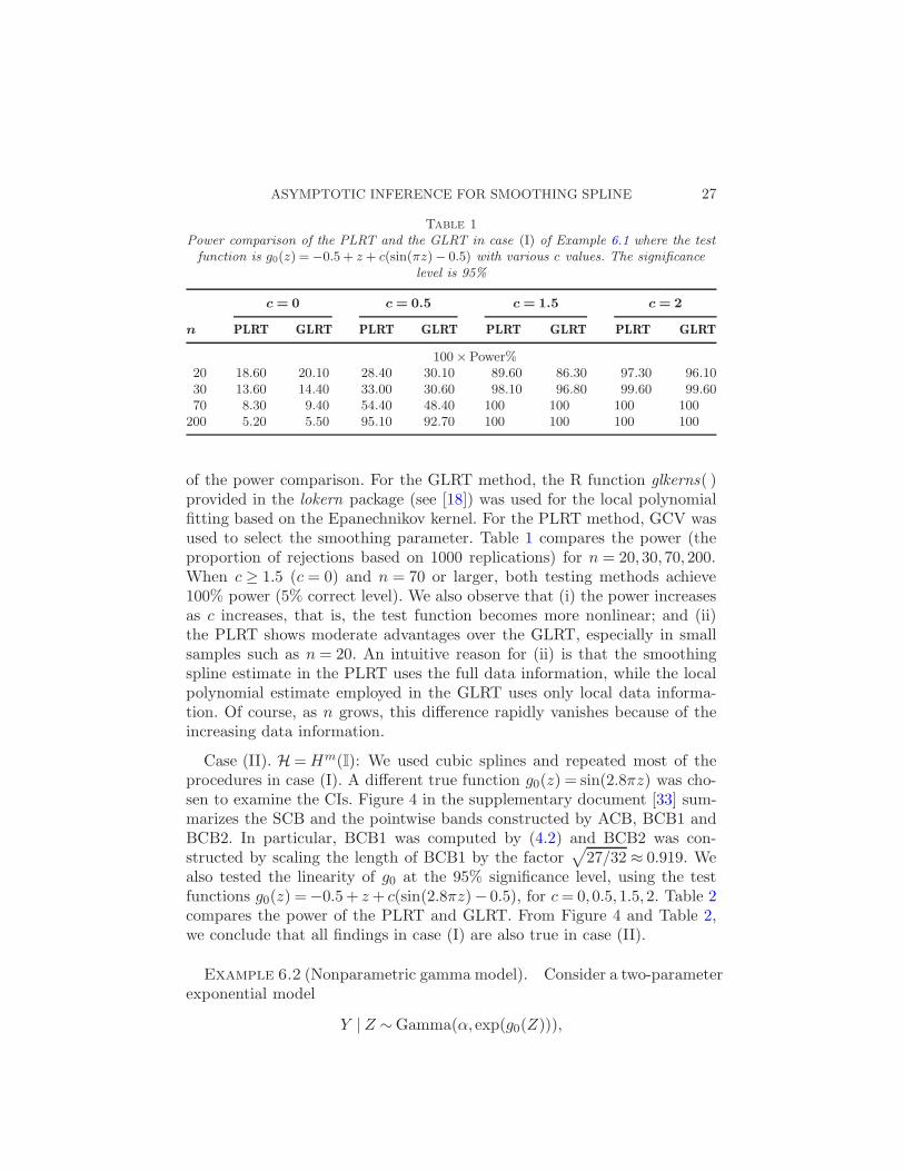
Table 1
Power comparison of the PLRT and the GLRT in case (I) of Example 6.1 where the testfunction is g0(z) =−0.5+ z + c(sin(πz)− 0.5) with various c values. The significance
level is 95%
c= 0 c= 0.5 c= 1.5 c= 2
n PLRT GLRT PLRT GLRT PLRT GLRT PLRT GLRT
100×Power%20 18.60 20.10 28.40 30.10 89.60 86.30 97.30 96.1030 13.60 14.40 33.00 30.60 98.10 96.80 99.60 99.6070 8.30 9.40 54.40 48.40 100 100 100 100
200 5.20 5.50 95.10 92.70 100 100 100 100
of the power comparison. For the GLRT method, the R function glkerns( )provided in the lokern package (see [18]) was used for the local polynomialfitting based on the Epanechnikov kernel. For the PLRT method, GCV wasused to select the smoothing parameter. Table 1 compares the power (theproportion of rejections based on 1000 replications) for n = 20,30,70,200.When c ≥ 1.5 (c = 0) and n = 70 or larger, both testing methods achieve100% power (5% correct level). We also observe that (i) the power increasesas c increases, that is, the test function becomes more nonlinear; and (ii)the PLRT shows moderate advantages over the GLRT, especially in smallsamples such as n = 20. An intuitive reason for (ii) is that the smoothingspline estimate in the PLRT uses the full data information, while the localpolynomial estimate employed in the GLRT uses only local data informa-tion. Of course, as n grows, this difference rapidly vanishes because of theincreasing data information.
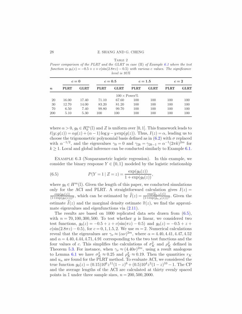
Case (II). H=Hm(I): We used cubic splines and repeated most of theprocedures in case (I). A different true function g0(z) = sin(2.8πz) was cho-sen to examine the CIs. Figure 4 in the supplementary document [33] sum-marizes the SCB and the pointwise bands constructed by ACB, BCB1 andBCB2. In particular, BCB1 was computed by (4.2) and BCB2 was con-structed by scaling the length of BCB1 by the factor
√27/32 ≈ 0.919. We
also tested the linearity of g0 at the 95% significance level, using the testfunctions g0(z) =−0.5+ z+ c(sin(2.8πz)− 0.5), for c= 0,0.5,1.5,2. Table 2compares the power of the PLRT and GLRT. From Figure 4 and Table 2,we conclude that all findings in case (I) are also true in case (II).
Example 6.2 (Nonparametric gamma model). Consider a two-parameterexponential model
Y | Z ∼Gamma(α, exp(g0(Z))),
28 Z. SHANG AND G. CHENG
Table 2
Power comparison of the PLRT and the GLRT in case (II) of Example 6.1 where the testfunction is g0(z) =−0.5 + z + c(sin(2.8πz)− 0.5) with various c values. The significance
level is 95%
c= 0 c= 0.5 c= 1.5 c= 2
n PLRT GLRT PLRT GLRT PLRT GLRT PLRT GLRT
100×Power%20 16.00 17.40 71.10 67.60 100 100 100 10030 12.70 14.00 83.20 81.20 100 100 100 10070 6.50 7.40 99.80 99.70 100 100 100 100
200 5.10 5.30 100 100 100 100 100 100
where α > 0, g0 ∈Hm0 (I) and Z is uniform over [0,1]. This framework leads to
ℓ(y;g(z)) = αg(z) + (α− 1) log y− y exp(g(z)). Thus, I(z) = α, leading us tochoose the trigonometric polynomial basis defined as in (6.2) with σ replacedwith α−1/2, and the eigenvalues γ0 = 0 and γ2k = γ2k−1 = α−1(2πk)2m fork ≥ 1. Local and global inference can be conducted similarly to Example 6.1.
Example 6.3 (Nonparametric logistic regression). In this example, weconsider the binary response Y ∈ {0,1} modeled by the logistic relationship
P (Y = 1 | Z = z) =exp(g0(z))
1 + exp(g0(z)),(6.5)
where g0 ∈Hm(I). Given the length of this paper, we conducted simulationsonly for the ACI and PLRT. A straightforward calculation gives I(z) =
exp(g0(z))(1+exp(g0(z)))2
, which can be estimated by I(z) =exp(gn,λ(z))
(1+exp(gn,λ(z)))2. Given the
estimate I(z) and the marginal density estimate π(z), we find the approxi-mate eigenvalues and eigenfunctions via (2.11).
The results are based on 1000 replicated data sets drawn from (6.5),with n = 70,100,300,500. To test whether g is linear, we considered twotest functions, g0(z) = −0.5 + z + c(sin(πz) − 0.5) and g0(z) = −0.5 + z +c(sin(2.8πz)− 0.5), for c= 0,1,1.5,2. We use m= 2. Numerical calculationsreveal that the eigenvalues are γν ≈ (αν)2m, where α= 4.40,4.41,4.47,4.52and α= 4.40,4.44,4.71,4.91 corresponding to the two test functions and thefour values of c. This simplifies the calculations of σ2K and ρ2K defined inTheorem 5.3. For instance, when γν ≈ (4.40ν)2m , using a result analogousto Lemma 6.1 we have σ2K ≈ 0.25 and ρ2K ≈ 0.19. Then the quantities rKand un are found for the PLRT method. To evaluate ACI, we considered thetrue function g0(z) = (0.15)106z11(1− z)6 +(0.5)104z3(1− z)10 − 1. The CPand the average lengths of the ACI are calculated at thirty evenly spacedpoints in I under three sample sizes, n= 200,500,2000.

ASYMPTOTIC INFERENCE FOR SMOOTHING SPLINE 29
Table 3
Power of PLRT in Example 6.3 where the testfunction is g0(z) =−0.5 + z + c(sin(πz)− 0.5) with
various c values. The significance level is 95%
n c= 0 c= 1 c= 1.5 c= 2
100×Power%70 4.10 16.90 30.20 50.80
100 4.50 17.30 38.90 63.40300 5.00 52.50 92.00 99.30500 5.00 79.70 99.30 100
Table 4
Power of PLRT in Example 6.3 where the testfunction is g0(z) =−0.5 + z+ c(sin(2.8πz)− 0.5) with
various c values. The significance level is 95%
n c= 0 c= 1 c= 1.5 c= 2
100×Power%70 4.10 56.20 90.10 99.00
100 5.00 71.90 96.90 100300 5.00 99.80 100 100500 5.00 100 100 100
The results on the power of the PLRT are summarized in Tables 3 and 4,which demonstrate the validity of the proposed testing method. Specifically,when c= 0, the power reduces to the desired size 0.05; when c ≥ 1.5 andn ≥ 300, the power approaches one. The results for the CPs and averagelengths of ACIs are summarized in Figure 2. The CP uniformly approachesthe desired 95% confidence level as n grows, showing the validity of theintervals.
Acknowledgement. We are grateful for helpful discussions with ProfessorChong Gu and careful proofreading of Professor Pang Du. The authors alsothank the Co-Editor Peter Hall, the Associate Editor, and two referees forinsightful comments that led to important improvements in the paper.
SUPPLEMENTARY MATERIAL
Supplement to “Local and global asymptotic inference in smoothing spline
models” (DOI: 10.1214/13-AOS1164SUPP; .pdf). The supplementary ma-terials contain all the proofs of the theoretical results in the present paper.

30 Z. SHANG AND G. CHENG
Fig. 2. The first panel displays the true function g0(z) = (0.15)106z11(1 − z)6 +(0.5)104z3(1− z)10 − 1 used in Example 6.3. The other panels contain the CP and averagelength (number in the plot title) of each ACI. The ACIs were built upon thirty equallyspaced covariates.
REFERENCES
[1] Banerjee, M. (2007). Likelihood based inference for monotone response models.Ann. Statist. 35 931–956. MR2341693
[2] Bickel, P. J. and Rosenblatt, M. (1973). On some global measures of the devia-tions of density function estimates. Ann. Statist. 1 1071–1095. MR0348906
[3] Birkhoff, G. D. (1908). Boundary value and expansion problems of ordinary lineardifferential equations. Trans. Amer. Math. Soc. 9 373–395. MR1500818
[4] Chen, J. C. (1994). Testing goodness of fit of polynomial models via spline smoothingtechniques. Statist. Probab. Lett. 19 65–76. MR1253314
[5] Claeskens, G. and Van Keilegom, I. (2003). Bootstrap confidence bands for re-gression curves and their derivatives. Ann. Statist. 31 1852–1884. MR2036392
ASYMPTOTIC INFERENCE FOR SMOOTHING SPLINE 31
[6] Cox, D., Koh, E., Wahba, G. and Yandell, B. S. (1988). Testing the (parametric)null model hypothesis in (semiparametric) partial and generalized spline models.
Ann. Statist. 16 113–119. MR0924859[7] Cox, D. D. and O’Sullivan, F. (1990). Asymptotic analysis of penalized likelihood
and related estimators. Ann. Statist. 18 1676–1695. MR1074429
[8] Davis, P. J. (1963). Interpolation and Approximation. Blaisdell, New York.MR0157156
[9] Fan, J., Zhang, C. and Zhang, J. (2001). Generalized likelihood ratio statistics andWilks phenomenon. Ann. Statist. 29 153–193. MR1833962
[10] Fan, J. and Zhang, J. (2004). Sieve empirical likelihood ratio tests for nonparametric
functions. Ann. Statist. 32 1858–1907. MR2102496[11] Fan, J. and Zhang, W. (2000). Simultaneous confidence bands and hypothesis test-
ing in varying-coefficient models. Scand. J. Stat. 27 715–731. MR1804172[12] Genovese, C. and Wasserman, L. (2008). Adaptive confidence bands. Ann. Statist.
36 875–905. MR2396818
[13] Gu, C. (2002). Smoothing Spline ANOVA Models. Springer, New York. MR1876599[14] Gu, C. and Qiu, C. (1993). Smoothing spline density estimation: Theory. Ann.
Statist. 21 217–234. MR1212174[15] Hall, P. (1991). Edgeworth expansions for nonparametric density estimators, with
applications. Statistics 22 215–232. MR1097375
[16] Hall, P. (1992). Effect of bias estimation on coverage accuracy of bootstrap confi-dence intervals for a probability density. Ann. Statist. 20 675–694. MR1165587
[17] Hardle, W. (1989). Asymptotic maximal deviation of M -smoothers. J. MultivariateAnal. 29 163–179. MR1004333
[18] Herrmann, E. (1997). Local bandwidth choice in kernel regression estimation.
J. Comput. Graph. Statist. 6 35–54. MR1451989[19] Ingster, Y. I. (1993). Asymptotically minimax hypothesis testing for nonparametric
alternatives I–III. Math. Methods Statist. 2 85–114; 3 171–189; 4, 249–268.[20] Jayasuriya, B. R. (1996). Testing for polynomial regression using nonparametric
regression techniques. J. Amer. Statist. Assoc. 91 1626–1631. MR1439103
[21] Ke, C. and Wang, Y. (2002). ASSIST: A suite of S-plus functions implementingspline smoothing techniques. Preprint.
[22] Krivobokova, T., Kneib, T. and Claeskens, G. (2010). Simultaneous confidencebands for penalized spline estimators. J. Amer. Statist. Assoc. 105 852–863.MR2724866
[23] Liu, A. andWang, Y. (2004). Hypothesis testing in smoothing spline models. J. Stat.Comput. Simul. 74 581–597. MR2074614
[24] Mammen, E. and van de Geer, S. (1997). Penalized quasi-likelihood estimation inpartial linear models. Ann. Statist. 25 1014–1035. MR1447739
[25] McCullagh, P. and Nelder, J. A. (1989). Generalized Linear Models, 2nd ed.
Chapman & Hall, London. MR0727836[26] Messer, K. and Goldstein, L. (1993). A new class of kernels for nonparametric
curve estimation. Ann. Statist. 21 179–195. MR1212172[27] Neumann, M. H. and Polzehl, J. (1998). Simultaneous bootstrap confidence bands
in nonparametric regression. J. Nonparametr. Stat. 9 307–333. MR1646905
[28] Nychka, D. (1988). Bayesian confidence intervals for smoothing splines. J. Amer.Statist. Assoc. 83 1134–1143. MR0997592
[29] Nychka, D. (1995). Splines as local smoothers. Ann. Statist. 23 1175–1197.MR1353501

32 Z. SHANG AND G. CHENG
[30] Ramil Novo, L. A. and Gonzalez Manteiga, W. (2000). F tests and regressionanalysis of variance based on smoothing spline estimators. Statist. Sinica 10
819–837. MR1787781[31] Rice, J. and Rosenblatt, M. (1983). Smoothing splines: Regression, derivatives
and deconvolution. Ann. Statist. 11 141–156. MR0684872[32] Shang, Z. (2010). Convergence rate and Bahadur type representation of general
smoothing spline M-estimates. Electron. J. Stat. 4 1411–1442. MR2741207[33] Shang, Z. and Cheng, G. (2013). Supplement to “Local and global asymptotic
inference in smoothing spline models.” DOI:10.1214/13-AOS1164SUPP.[34] Shao, J. (2003). Mathematical Statistics, 2nd ed. Springer, New York. MR2002723[35] Silverman, B. W. (1984). Spline smoothing: The equivalent variable kernel method.
Ann. Statist. 12 898–916. MR0751281[36] Stone, M. H. (1926). A comparison of the series of Fourier and Birkhoff. Trans.
Amer. Math. Soc. 28 695–761. MR1501372[37] Sun, J., Loader, C. and McCormick, W. P. (2000). Confidence bands in general-
ized linear models. Ann. Statist. 28 429–460. MR1790004[38] Sun, J. and Loader, C. R. (1994). Simultaneous confidence bands for linear regres-
sion and smoothing. Ann. Statist. 22 1328–1345. MR1311978[39] Utreras, F. I. (1988). Boundary effects on convergence rates for Tikhonov regular-
ization. J. Approx. Theory 54 235–249. MR0960047[40] Wahba, G. (1983). Bayesian “confidence intervals” for the cross-validated smoothing
spline. J. R. Stat. Soc. Ser. B Stat. Methodol. 45 133–150. MR0701084[41] Wahba, G. (1990). Spline Models for Observational Data. SIAM, Philadelphia, PA.
MR1045442[42] Wang, Y. (2011). Smoothing Splines: Methods and Applications. Monographs on
Statistics and Applied Probability 121. Chapman & Hall/CRC Press, Boca Ra-ton, FL. MR2814838
[43] Wedderburn, R. W. M. (1974). Quasi-likelihood functions, generalized linear mod-els, and the Gauss–Newton method. Biometrika 61 439–447. MR0375592
[44] Zhang, W. and Peng, H. (2010). Simultaneous confidence band and hypothesis testin generalised varying-coefficient models. J. Multivariate Anal. 101 1656–1680.MR2610738
[45] Zhou, S., Shen, X. and Wolfe, D. A. (1998). Local asymptotics for regressionsplines and confidence regions. Ann. Statist. 26 1760–1782. MR1673277
University of Notre Dame
Notre Dame, Indiana 46556
USA
E-mail: [email protected]
Department of Statistics
Purdue University
250 N. University St.
West Lafayette, Indiana 47906
USA
E-mail: [email protected]

Submitted to the Annals of Statistics
Supplementary document to
LOCAL AND GLOBAL ASYMPTOTIC INFERENCE IN SMOOTHING
SPLINE MODELS
By Zuofeng Shang‡ and Guang Cheng§
University of Notre Dame and Purdue University
August 27, 2013
In this document, we first give a table that lists the notation of the paper, and then give the
proofs. In particular, we describe and prove the minimax results for the PLRT.
We organize this document as follows:
• In Section S.1, we give a table defining our notation, and indicating the page numbers of the
first occurences.
• Sections S.2, S.3, and S.4 include the proofs of Proposition 2.1, Proposition 2.2, and Lemma
3.1.
• In Section S.5, we prove the concentration inequality in Lemma 3.2.
• In Section S.6, we prove Proposition 3.3, i.e., the convergence rate of gn,λ.
• In Section S.7, we prove Theorem 3.4, i.e., the FBR. In Section S.8, we prove the pointwise
asymptotic normality of the smoothing spline estimate in Theorem 3.5.
• In Section S.9, we prove Corollary 3.7 on the pointwise asymptotic normality of gn,λ in L2
regression.
• In Section S.10, we sketch the proof of another technical tool, i.e., the restricted FBR in
Theorem 4.3, which is used to establish the asymptotic null distribution of the local LRT.
• In Section S.11, we show the Wilks phenomenon of the local LRT.
• In Section S.12, we prove Corollary 4.5.
• In Section S.13, we demonstrate the validity of the proposed SCB.
• In Section S.14, we prove Proposition 5.2, i.e., the equivalent kernel conditions.
• In Section S.15, we derive the null limiting distribution of the PLRT.
‡Postdoctoral Fellow.§Corresponding Author. Associate Professor. Research Sponsored by NSF, DMS-0906497, and CAREER Award
DMS-1151692
31

32 Z. SHANG AND G. CHENG
• In Section S.16, we prove Theorem 5.4, i.e., when the data are normal, the PLRT attains the
optimal minimax rates of testing. We further extend this result to a more general modeling
framework in Section S.17.
• In Section S.18, we show Lemma 6.1.
• We give two figures for Example 6.1 showing the performance of the proposed ACI and SCB.
The reference labels of the equations, theorems, propositions, and lemmas in this document are
consistent with those in the main text of the paper.

ASYMPTOTIC INFERENCE FOR SMOOTHING SPLINE 33
Notation Meaning First appearing in page No.Y response 4Z covariate 4T T = (Y, Z) denotes the full data variable 4Y range of Y 4I I = [0, 1] denotes the range of Z 4F the link function 4g0 the true function 4
Q(y;µ) the quasi-likelihood function 4`(y; a) the general criteria function 4m the roughness degree of g0 4
J(·, ·) the penalty function 4H the parameter space for g 4
Hm(I) the Sobolev space on [0, 1] 4Hm0 (I) the homogeneous Sobolev space on [0, 1] 4`n,λ the penalized empirical criteria function 4gn,λ the unconstrained estimate of g 4λ the smoothing parameter 4Nm the null space for J 4I0 the range of g0 4I a bounded open interval including I0 4
˙a, ¨
a, `′′′a the first-, second- and third-order partial derivatives w.r.t. a 4
I(Z) −E{¨a(Y ; g0(Z))|Z} 5〈·, ·〉, ‖ · ‖ the inner product and norm 5
K the reproducing kernel function 6Kz the function determined by Kz(·) = K(z, ·) 6V V (g, g) = E{I(Z)g(Z)g(Z)} 6Wλ the penalty operator 6id the identity operator 6
aν � bν asymptotically equivalent 6aν ∼ bν asymptotically equal 6‖ · ‖sup the supremum norm 6γν the eigenvalue 6hν the eigenfunction function corresponding to γν 6D the Frechet differential operator 7Sn,λ = D`n,λ 7
h = λ1/(2m) 7‖ · ‖H a norm stronger than ‖ · ‖ 8
λ∗ a sequence satisfying λ∗ � n−2m/(2m+1) 8
h∗ = (λ∗)1/(2m) 8g∗0 = (id−Wλ)g0 9
σ2z0
the asymptotic variance of gn,λ(z0) 9
bz0 the asymptotic estimation bias of gn,λ(z0) 9
h† = hσ1/m 11I1, I2 two explicit integrals 11
a(h†) a quantity introduced by Wahba (1983) 12
g0n,λ the optimizer constrained with g(z0) = 0 13
H0 a subspace of H with restriction g(z0) = 0 13K∗ a restricted version of K in H0 13W∗λ a restricted version of Wλ in H0 13rn rate of convergence 14c0 a scaling constant in local LRT 14ω(·) an equivalent kernel function 15ω0 an equivalent kernel function in the specific L2 regression 17
rK , ρK , σ2K , un constants in the PLRT 19
σ2 estimated variance 22
Table 5A table that lists all useful notation, their meanings and where they first appear.
S.1. Notation Table.

34 Z. SHANG AND G. CHENG
S.2. Proof of Proposition 2.1. Based on the definition (2.8), we can write ‖g‖2 = V (g, g) +
λJ(g, g), and then plug in the Fourier expansion of g to obtain the explicit expression of ‖g‖2. A
direct calculation reveals that
(S.1) 〈g, hν〉 = 〈∑µ
V (g, hµ)hµ, hν〉 = V (g, hν)(1 + λγν),
for any g ∈ H and ν ∈ N. It follows by (S.1) that V (Kz, hν) = 〈Kz, hν〉/(1+λγν) = hν(z)/(1+λγν).
Hence, we can obtain the expression of Kz(·) by using Kz(·) =∑
ν V (Kz, hν)hν(·). Furthermore,
(S.1) implies that V (Wλhν , hµ) = 〈Wλhν , hµ〉/(1 + λγµ) = λγµδµν/(1 + λγµ), for any ν, µ ∈ N.
Finally, we can conclude the proof of Proposition 2.1 by using Wλhν(·) =∑
µ V (Wλhν , hµ)hµ.
S.3. Proof of Proposition 2.2. The usual L2-inner product is defined to be 〈g, ξ〉L2 =∫ 1
0 g(z)ξ(z)dz.
Let D be the differential operator, i.e., Dφ = ddzφ, and ω = 1/(Iπ). Thus, ω ∈ Cm(I) is positive and
finitely upper bounded. It follows from [5] that the growing rate for γν is of order ν2m. Since the
operator L0 = (−1)mωD2m is self-adjoint under the inner product V , that is, V (L0g, ξ) = V (g, L0ξ)
for any ξ, g ∈ C2m(I) satisfying the boundary conditions in (2.11), orthogonality and completeness
of hν under V thus follow from Theorem 2.1 (pp. 189) and Theorem 4.2 (pp. 199) of [8] with the
usual L2-inner product 〈, 〉L2 replaced with V . Therefore, when hν are normalized to V (hν , hν) = 1,
they form an orthonormal and complete set in L2(I;V ).
Next we show that h(m)ν , ν ≥ m, are complete in L2(I) under 〈, 〉L2 . The idea follows from argu-
ments on page 147 of [31]. The eigenspace corresponding to the zero eigenvalue contains functions φ
that satisfy (−1)mφ(2m) = 0 with boundary conditions φ(j)(0) = φ(j)(1) = 0 for j = m, . . . , 2m− 1,
thus it follows from [49] that this eigenspace is Pm−1, i.e., the set of all polynomials of degree
at most m − 1. Let hν , ν = 0, . . . ,m − 1, be the orthonormal basis (under V ) of Pm−1 corre-
sponding to γ0 = . . . = γm−1 = 0. Note γν > 0 for ν ≥ m. For g ∈ L2(I) such that for any
ν ≥ m,∫ 1
0 gh(m)ν = 0, let ξ be a solution of ξ(m) = g, then using integration by parts we have
0 =∫ 1
0 ξh(2m)ν = (−1)mγνV (ξ, hν). Therefore V (ξ, hν) = 0 for any ν ≥ m. By completeness of
hν , ξ must be a linear combination of h0, . . . , hm−1, a polynomial with degree at most m − 1. So
g = ξ(m) = 0 implying the completeness of h(m)ν /γ
1/2ν for ν ≥ m in L2(I) under 〈, 〉L2 . Now, for
any g ∈ H, by completeness of hν in L2(I) under V -norm, g =∑
ν∈N V (g, hν)hν with convergence
in V -norm. Since V (g, hν) =∫ 1
0 g(m)h
(m)ν /γν , by completeness of h
(m)ν /γ
1/2ν for ν ≥ m in L2(I) in
usual ‖ · ‖L2-norm, g(m) =∑
ν≥m〈g(m), h(m)ν 〉L2h
(m)ν /γν =
∑ν≥m V (g, hν)h
(m)ν with convergence in
usual L2-norm. This implies g =∑
ν V (g, hν)hν converges in ‖ · ‖.
Next we show the uniform boundedness of hν . We only consider those hν corresponding to
nonzero γν . If γν 6= 0 and hν satisfy (−1)mh(2m)ν = γνIπhν and V (hν , hν) = 1, then using the

ASYMPTOTIC INFERENCE FOR SMOOTHING SPLINE 35
boundary conditions in (2.11) and integration by parts, one can check that J(hν , hν) = γν . Dividing
Iπ and taking m-order derivatives on both sides, one obtains Lh(m)ν = γνh
(m)ν with h
(m+j)ν (0) =
h(m+j)ν (1) = 0, j = 0, . . . ,m − 1, where L = (−1)m
∑mj=0
(mj
)ω(j)D2m−j . Therefore, h
(m)ν is an
eigenfunction of L with eigenvalue γν . Denote the eigenfunctions and eigenvalues of L to be ψν and
λν subject to ψ(j)ν (0) = ψ
(j)ν (1) = 0, j = 0, . . . ,m− 1. We need to transform L to normal form. Let
t(z) =∫ z
0 [I(s)π(s)]1/(2m)ds/C and C =∫ 1
0 [I(z)π(z)]1/(2m)dz. Define φν(t(z)) = ψν(z). Then by a
direct examination, φν satisfies the following differential equation
(S.2)
φ(2m)ν (t) + q2m−1(t)φ(2m−1)
ν (t) + . . .+ q0(t)φν(t) = ρνφν(t), φ(j)ν (0) = φ(j)
ν (1) = 0, j = 0, . . . ,m− 1
where qj , j = 0, . . . , 2m−1, are coefficient functions depending only on Iπ and m, and ρν = λνC2m.
In general the form of qj are complicated though they can be determined by Faa di Bruno’s
formula ([25]). As an illustration, when m = 2, q0(t) = 0, q3(t) = −(C/4)ω(1)(z(t))ω(z(t))−3/4,
q2(t) = −(C2/4)(ω(1)(z(t)))2ω(z(t))−3/2, and
q1(t) = C3(−5ω(z(t))−9/4(ω(1)(z(t)))3/64+3ω(z(t))−5/4ω(1)(z(t))ω(2)(z(t))/16−ω(z(t))−1/4ω(3)(z(t))),
where z(t) is the inverse function of t(z) and b2(z) = [I(z)π(z)]1/4. Define
(S.3) uν(t) = φν(t) exp
(1
2m
∫ t
0q2m−1(s)ds
),
then (S.2) is equivalent to
(S.4) Luν ≡ u(2m)ν (t) + p2m−2(t)u(2m−2)
ν + . . .+ p0(t)uν(t) = ρνuν(t),
with the boundary conditions u(j)ν (0) = u
(j)ν (1) = 0, j = 0, . . . ,m − 1. Note (S.4) is the classic
form of differential systems discussed in [5]. According to [5], ρν are simple due to the regular
boundary conditions, and the residual of the Green function G(z1, z2; ρ) for L − ρI at pole ρν is
given by uν(t1)uν(t2)‖uν‖2L2
, where ‖ · ‖L2 denotes the usual L2-norm. On the other hand, the residue can
also be represented by 12π√−1
∫Γρν
2mζ2m−1G(t1, t2, ζ2m)dζ (pp. 722, [45]), where ζ = ρ1/(2m), Γρν
denotes the contour centered around pole ρν with suitably small radius. By equation (56) and the
discussions below in [5], 2mζ2m−1G(t1, t2; ζ2m) is uniformly bounded for t1, t2 ∈ I, thus the residue
is uniformly bounded for all t1, t2. In particular, letting t1 = t2 = t, we get |uν(t)| ≤ c‖uν‖L2 for
any t ∈ I with a universal constant c > 0. Since q2m−1 achieves finite upper and lower bounds on I,
by (S.3), there is a universal constant c1 > 0 such that for any ν, ‖φν‖sup ≤ c1‖φν‖L2 . Now, using
φν(t(z)) = ψν(z), we get
‖ψν‖2sup = ‖φν‖2sup ≤ c21‖φν‖2L2
= c21
∫ 1
0|φν(t)|2dt = c2
1
∫ 1
0|φν(t(z))|2|I(z)π(z)|1/(2m)dz ≤ c2
1c2Iπ‖ψν‖2L2
,

36 Z. SHANG AND G. CHENG
where cIπ is a constant depending only on Iπ and m. So ‖ψν‖sup ≤ c1cIπ‖ψν‖L2 . Letting ψν = h(m)ν
and using the fact that ‖h(m)ν ‖2L2
= γν , we have ‖h(m)ν ‖sup ≤ c1cIπγ
1/2ν , for any ν ∈ N.
By the Sobolev embedding theorem ([1]), ‖hν‖2sup ≤ c2(V (hν , hν) + J(hν , hν)) = c2(1 + γν). By
Theorem 5 of [49], for any j = 1, . . . ,m, there is a constant Cj > 0 such that ‖h(j)ν ‖sup ≤ Cj(1 +
γν)1/2, ∀ν ∈ N. Therefore, taking the mth-order derivative on both sides of (−1)mh(2m)ν = γνIπhν ,
one can show that ‖h(3m)ν ‖sup ≤ γν
∑mj=0
(mj
)‖(Iπ)(m−j)‖sup · ‖h(j)
ν ‖sup ≤ c2(1 + γν)3/2 for some
constant c2 > 0 and any ν. Again, by Theorem 5 of [49] for h(m)ν and ε = γ
−1/(2m)ν , we have
‖h(2m)ν ‖sup ≤ C ′m(1 + γν), which implies ‖hν‖sup ≤ C ′m(infz |I(z)|)−1(1 + γν)/γν ≤ C ′′m, with a
universal constant C ′′m unrelated to ν. This proves the desired uniform boundedness of hν .
S.4. Proof of Lemma 3.1. For any z ∈ I, |〈Kz, g〉| ≤ ‖Kz‖ · ‖g‖. So, we only need to find the
upper bound for ‖Kz‖. By Proposition 2.1 and the boundedness of hµ, we have
(S.5) ‖Kz‖2 = K(z, z) =∑µ∈Z
|hµ(z)|2
1 + λγµ≤ C
∑µ∈Z
1
1 + λγµ≤ c2
mλ−1/(2m) = c2
mh−1,
where cm > 0 is a constant that does not rely on z and h. So ‖Kz‖ ≤ cmh−1/2.
S.5. Proof of Lemma 3.2. For any g, f ∈ G, by Lemma 3.1,
‖(ψn(T ; f)− ψn(T ; g))KZ‖ ≤ c−1m h1/2‖f − g‖sup · ‖KZ‖
≤ c−1m h1/2‖f − g‖sup · cmh−1/2 = ‖f − g‖sup.
By Theorem 3.5 of [38], for any t > 0, P (‖Zn(f)− Zn(g)‖ ≥ t) ≤ 2 exp(− t2
8‖f−g‖2sup
). Then by
Lemma 8.1 in [27], we have ‖‖Zn(g)− Zn(f)‖‖ψ2≤ 8‖g − f‖sup, where ‖ · ‖ψ2 denotes the Orlicz
norm associated with ψ2(s) ≡ exp(s2)−1. It follows by Theorem 8.4 of [27] that for arbitrary δ > 0,∥∥∥∥∥∥∥ supg,f∈G
‖g−f‖sup≤δ
‖Zn(g)− Zn(f)‖
∥∥∥∥∥∥∥ψ2
≤ C ′(∫ δ
0
√log(1 +N(δ,G, ‖ · ‖sup)) + δ
√log(1 +N(δ,G, ‖ · ‖sup)2)
)
� h−(2m−1)/(4m)δ1−1/(2m).
So, again, by Lemma 8.1 in [27],
(S.6) P
supg∈G
‖g‖sup≤δ
‖Zn(g)‖ ≥ t
≤ 2 exp(−h(2m−1)/(2m)δ−2+1/mt2).
Let bn = n1/2h−(2m−1)/(4m), ε = b−1n , γ = 1−1/(2m), Tn = (5 log log n)1/2, and Qε = [− log ε−1],
ASYMPTOTIC INFERENCE FOR SMOOTHING SPLINE 37
where [a] denotes the integer part of a. Then by (S.6),
P
(supg∈G
√n‖Zn(g)‖
an‖g‖γsup + 1≥ Tn
)≤ P
supg∈G
‖g‖sup≤ε1/γ
√n‖Zn(g)‖
an‖g‖γsup + 1≥ Tn
+
Qε∑l=0
P
supg∈G
(2lε)1/γ≤‖g‖sup≤(2l+1ε)1/γ
√n‖Zn(g)‖
an‖g‖γsup + 1≥ Tn
≤ P
supg∈G
‖g‖sup≤ε1/γ
√n‖Zn(g)‖ ≥ Tn
+
Qε∑l=0
P
supg∈G
‖g‖sup≤(2l+1ε)1/γ
√n‖Zn(g)‖ ≥ (1 + 2l)Tn
≤ 2 exp
(−h(2m−1)/(2m)(ε1/γ)−2+1/mT 2
n/n)
+
Qε∑l=0
2 exp(−h(2m−1)/(2m)[(2l+1ε)1/γ ]−2+1/mT 2
n(2l + 1)2/n)
= 2 exp(−T 2
n
)+
Qε∑l=0
2 exp(−2−2(l+1)T 2
n(2l + 1)2)
≤ 2(Qε + 2) exp(−T 2/4
)≤ const · log n(log n)−5/4 → 0,
as n→∞. This proves the result.
S.6. Proof of Proposition 3.3. To prove Proposition 3.3, we first need the following Lemma.
Denote N(δ,G, ‖ · ‖sup) as the δ-covering number of the function class G in terms of the uniform
norm.
Lemma S.1. Suppose that c−2m hλ−1 > 1. Then, for any δ > 0, we have
logN(δ,G, ‖ · ‖sup) ≤ C(hλ−1)1/(2m)δ−1/m,
where C > 0 is an universal constant.
Proof of Lemma S.1. Note that by c−2m hλ−1 > 1,
G = (c−2m hλ−1)1/2 · {g ∈ H|‖g‖sup ≤ (c−2
m hλ−1)−1/2, J(g, g) ≤ 1} ⊂ (c−2m hλ−1)1/2T ,

38 Z. SHANG AND G. CHENG
where T = {g ∈ H|‖g‖sup ≤ 1, J(g, g) ≤ 1}. So, by [27], we have
logN(δ,G, ‖ · ‖sup) ≤ logN(δ, (c−2m hλ−1)1/2T , ‖ · ‖sup)
= logN((c−2m hλ−1)−1/2δ, T , ‖ · ‖sup)
≤ c((c−2m hλ−1)−1/2δ)−1/m = cc−1/m
m (hλ−1)1/(2m)δ−1/m.
Consider the function class F = {g ∈ H|‖g‖sup ≤ 1, J(g, g) ≤ 1}. By Lemma S.1, for any δ > 0,
we know logN(δ,F , ‖ · ‖sup) ≤ cδ−1/m, where c is some universal constant. Then a modification of
Lemma 3.2 leads to
Lemma S.2. Suppose that ψn satisfies the following Lipschitz continuity condition, i.e.,
(S.7) |ψn(T ; f)− ψn(T ; g)| ≤ c−1m h1/2‖f − g‖sup, for all f, g ∈ F ,
where cm is specified in Lemma 3.1. Then we have
limn→∞
P
(supg∈F
‖Zn(g)‖‖g‖1−1/(2m)
sup + n−1/2≤ (5 log log n)1/2
)= 1,
where the empirical process Zn(g) is defined in (3.1).
Denote g = gn,λ − g0. By consistency of gn,λ in ‖ · ‖H-norm and Sobolev embedding Theorem
(see [1]), we know that gn,λ(z) falls in I for any z ∈ I and large enough n. By Taylor’s expansion,
`n,λ(g0 + g)− `n,λ(g0) = Sn,λ(g0)g +1
2DSn,λ(g0)gg +
1
6D2Sn,λ(g?)ggg ≥ 0,
where g? = g0 + t?g for some t? ∈ [0, 1]. Denote the three terms on the right side of the above
equation by I1, I2, I3. Next we will study the rates for these terms. Denote Ai = {supa∈I |¨a(Yi; a)|+
supa∈I |`′′′a (Yi; a)| ≤ C log n}. By (2.4), we may choose C to be large so that ∩iAi has large proba-
bility and P (Aci ) = O(n−2). Then, on ∩iAi, we have
|6I3| ≤1
n
n∑i=1
supa∈I|`′′′a (Yi; a)| · |g(Zi)|3
≤ 1
n‖g‖sup
n∑i=1
supa∈I|`′′′a (Yi; a)| · g(Zi)
2
=1
n‖g‖sup〈
n∑i=1
ψ(Ti; g)KZi , g〉
=1
n‖g‖sup〈
n∑i=1
[ψ(Ti; g)KZi − E{ψ(T ; g)KZ}], g〉+ ‖g‖supE{ψ(T ; g)g(Z)},

ASYMPTOTIC INFERENCE FOR SMOOTHING SPLINE 39
where ψ(Ti; g) = supa∈I |`′′′a (Yi; a)|g(Zi)IAi . Let ψn(Ti; g) = (C log n)−1c−1m h1/2ψ(Ti; g), which sat-
isfies (S.7). Thus, by Lemma S.2, we have, with large probability give large n,
‖n∑i=1
[ψn(Ti; g)KZi − E{ψn(T ; g)KZ}]‖ ≤ (n1/2‖g‖1−1/(2m)sup + 1)(5 log log n)1/2.
So, by Cauchy’s inequality, we have∣∣∣∣〈 n∑i=1
[ψ(Ti; g)KZi − E{ψ(T ; g)KZ}], g〉∣∣∣∣ ≤ ‖g‖ · (n1/2‖g‖1−1/(2m)
sup + 1)(5 log log n)1/2.
On the other hand, by Assumption A.1 (a), we have
E{ψ(T ; g)g(Z)} ≤ E{supa∈I|`′′′a (Y ; a)|g(Z)2} ≤ 2C2
0C1‖g‖2.
By (n1/2h)−1(log log n)m/(2m−1)(log n)2m/(2m−1) = o(1), which implies (n1/2h)−1(log log n)1/2 log n =
o(1), we have
|6I3| ≤1
n‖g‖sup · ‖g‖(C log n)cmh
−1/2(n1/2‖g‖1−1/(2m)sup + 1)(5 log log n)1/2 + 2C2
0C1‖g‖sup · ‖g‖2
= c2mC′(n1/2h)−1(log log n)1/2(log n)‖g‖2 + 2C2
0C1‖g‖sup · ‖g‖2
= oP (1) · ‖g‖2.(S.8)
To approximate I2, by Cauchy’s inequality, we have∣∣∣∣E{¨a(Y ; g0(Z))IAcg(Z)2}∣∣∣∣ ≤ E{|¨a(Y ; g0(Z))|2IAcg(Z)4}1/2 · P (Ac)1/2
≤ O(1) · (log n)‖g‖sup‖g‖n−1 = ‖g‖2O((nh)−1/2) = o(1)‖g‖2.
By changing ψ and ψn in the proof of (S.8) to ψ(Ti; g) = ¨a(Yi; g0(Zi))gIAi and ψn(Ti; g) =
(C log n)−1c−1m h1/2ψ(Ti; g), and using an argument similar to the proof of (S.8), we have
|[DSn,λ(g0)− E{DSn,λ(g0)}]gg| ≤ Ccmh−1+1/(4m)n−1/2(log log n)1/2(log n)‖g‖2−1/(2m)
+Ccm(nh1/2)−1(log log n)1/2(log n)‖g‖+ oP (1)‖g‖2.
Thus,
2I2 = −‖g‖2 + Ccmh−1+1/(4m)n−1/2(log log n)1/2(log n)‖g‖2−1/(2m)
+Ccm(nh1/2)−1(log log n)1/2(log n)‖g‖+ oP (1)‖g‖2.(S.9)
Note that E{‖∑n
i=1 εiKZi‖2} = O(nh−1). By (S.44) in the main paper, we have
(S.10) ‖Sn,λ(g0)‖ = OP ((nh)−1/2 + λ1/2).

40 Z. SHANG AND G. CHENG
Combining (S.8), (S.9), and (S.10), and by (nh1/2)−1(log log n)1/2(log n) = o((nh)−1/2), we have
for some large C ′
(1 + oP (1))‖g‖2 ≤ C ′((nh)−1/2 + λ1/2)‖g‖+ Ccmh−1+1/(4m)n−1/2(log log n)1/2(log n)‖g‖2−1/(2m).
Solving this inequality, and using (n1/2h)−1(log log n)m/(2m−1)(log n)2m/(2m−1) = o(1), we get ‖g‖ =
OP ((nh)−1/2 + λ1/2).
S.7. Proof of Theorem 3.4. By Assumption A.1 (a), it is not difficult to check the following
(S.11) max1≤i≤n
supa∈I|¨a(Yi; a)| = OP (log n).
By (S.11), we can let C > C0 be sufficiently large so that the eventBn1 = {max1≤i≤n supa∈I |¨a(Yi; a)| ≤
C log n} has large probability. Denote g = gn,λ − g0. By Assumption A.3, the event Bn2 = {‖g‖ ≤
rn ≡M((nh)−1/2 +hm)} has large probability with some pre-selected large M . So Bn = Bn1 ∩Bn2
has a large probability. Define g = d−1n g, where dn = cmrnh
−1/2. Since h = o(1) and nh2 → ∞,
dn = o(1). Then by Lemma 3.1, on Bn, ‖g‖sup ≤ 1. Note that J(g, g) = d−2n λ−1(λJ(g, g)) ≤
d−2n λ−1‖g‖2 ≤ d−2
n λ−1r2n ≤ c−2
m hλ−1. Thus, when the event Bn holds, g is an element in G.
Define ψ(T ; g) = ˙a(Y ; g(Z) + g0(Z)) − ˙
a(Y ; g0(Z)). By the definition of Sn and a direct cal-
culation, one can verify that Sn(g + g0) − S(g + g0) − (Sn(g0) − S(g0)) = 1n
∑ni=1[ψ(Ti; g)KZi −
E{ψ(T ; g)KZ}]. Let ψn(T ; g) = C−1c−1m (log n)−1h1/2d−1
n ψ(T ; dng) and ψn(Ti; g) = ψn(Ti; g)IAi ,
where Ai = {supa∈I |¨a(Yi; a)| ≤ C log n} for i = 1, . . . , n. Observe that Bn implies ∩iAi.
Next we show that ψn satisfies (3.2). For any g1, g2 ∈ G, and z ∈ I, both g0(z) + dng1(z) and
g0(z) + dng2(z) fall in I when n is sufficiently large since g0(z) ∈ I0 and dn = o(1). Recall that I0
and I are specified in Assumption A.1. Therefore,
|ψn(Ti; dng1)− ψn(Ti; dng2)| = C−1c−1m (log n)−1h1/2d−1
n |ψ(Ti; g1)− ψ(Ti; g2)| · IAi
= C−1c−1m (log n)−1h1/2d−1
n
∣∣ ∫ g0(Zi)+dng1(Zi)
g0(Zi)
¨a(Yi; a) · IAida
−∫ g0(Zi)+dng1(Zi)
g0(Zi)
¨a(Yi; a) · IAida
∣∣≤ C−1c−1
m (log n)−1h1/2d−1n · dn‖g1 − g2‖sup · sup
a∈I|¨a(Yi; a)| · IAi
≤ C−1c−1m (log n)−1h1/2d−1
n · dn · C log n · ‖g1 − g2‖sup
= c−1m h1/2‖g1 − g2‖sup.
Thus, ψn satisfies (3.2). By Lemma 3.2, with large probability
(S.12) ‖n∑i=1
[ψn(Ti; g)KZi − E{ψn(T ; g)KZ}]‖ ≤ (n1/2h−(2m−1)/(4m) + 1)(5 log log n)1/2.

ASYMPTOTIC INFERENCE FOR SMOOTHING SPLINE 41
On the other hand, by Chebyshev’s inequality
P (Aci ) = exp(−(C/C0) log n)E{exp(supa∈I|¨a(Yi; a)|/C0)} ≤ C1n
−C/C0 .
Since h = o(1) and nh2 →∞, we may choose C to be large enough so that 21/2C−1C0C1(log n)−1n−C/(2C0) <
a′nh1/2d−1
n , where a′n = n−1/2((nh)−1/2 + hm)h−(6m−1)/(4m)(log log n)1/2. By (2.3), which implies
E{supa∈I |¨a(Yi; a)|∣∣Zi} ≤ 2C1C
20 , we have E{|ψ(T ; dng)|2} ≤ 2C1C
20d
2n on Bn, where the expecta-
tion is taken with respect to T = (Y,Z). So when n is large, by Chebyshev’s inequality, we have on
Bn,
‖E{ψn(Ti; g)KZi} − E{ψn(Ti; g)KZi}‖ = ‖E{ψn(Ti; g)KZi · IAci }‖
≤ C−1(log n)−1d−1n
(E{|ψ(Ti; dng)|2}
)1/2P (Aci )
1/2
≤ 21/2C−1C0C1(log n)−1n−C/(2C0)
≤ a′nh1/2d−1
n ,
where the expectation is taken with respect to Ti. Therefore, by (S.12) and on Bn, we have
‖Sn(g + g0)− S(g + g0)− (Sn(g0)− S(g0))‖
=Ccm(log n)h−1/2dn
n‖
n∑i=1
[ψn(Ti; g)KZi − E{ψn(T ; g)KZ}]‖
≤ Ccm(log n)h−1/2dnn
(‖n∑i=1
[ψn(Ti; g)KZi − E{ψn(T ; g)KZ}]‖
+n‖E{ψn(Ti; g)KZi} − E{ψn(Ti; g)KZi}‖)
≤ Ccm(log n)h−1/2dnn
· [(n1/2h−(2m−1)/(4m) + 1)(5 log log n)1/2 + na′nh1/2d−1
n ]
≤ C ′cma′n log n,(S.13)
for some constant C ′ > 0 that only depends on C, cm,M .
By Taylor’s expansion, the fact Sn,λ(g + g0) = 0, and Proposition 2.3, we have
‖Sn(g + g0)− S(g + g0)− (Sn(g0)− S(g0))‖
= ‖Sn,λ(g + g0)− Sλ(g + g0)− Sn,λ(g0) + Sλ(g0)‖
= ‖Sλ(g + g0) + Sn,λ(g0)− Sλ(g0)‖
= ‖DSλ(g0)g +
∫ 1
0
∫ 1
0sD2Sλ(g0 + ss′g)ggdsds′ + Sn,λ(g0)‖
= ‖ − g +
∫ 1
0
∫ 1
0sD2Sλ(g0 + ss′g)ggdsds′ + Sn,λ(g0)‖
≥ ‖ − g + Sn,λ(g0)‖ − ‖∫ 1
0
∫ 1
0sD2Sλ(g0 + ss′g)ggdsds′‖.

42 Z. SHANG AND G. CHENG
Therefore,
‖g − Sn,λ(g0)‖
≤ ‖Sn(g + g0)− S(g + g0)− (Sn(g0)− S(g0))‖+ ‖∫ 1
0
∫ 1
0sD2Sλ(g0 + ss′g)ggdsds′‖
≤ ‖Sn(g + g0)− S(g + g0)− (Sn(g0)− S(g0))‖+
∫ 1
0
∫ 1
0s‖D2Sλ(g0 + ss′g)gg‖dsds′.(S.14)
Next we find an upper bound for ‖D2Sλ(g0 +ss′g)gg‖. The Frechet derivative of DSλ is found to
beD2Sλ = D2S Therefore,D2Sλ(g0+ss′g)gg = D2S(g0+ss′g)gg = E{`′′′a (Y ; (g0+ss′g)(Z))g(Z)2KZ},
where the expectation is taken with respect to T . Hence, by (2.4) and on Bn, we have
‖D2Sλ(g0 + ss′g)gg‖ = ‖E{`′′′a (Y ; (g0 + ss′g)(Z))g(Z)2KZ}‖ ≤ E{E{supa∈I|`′′′a (Y ; a)|
∣∣Z}g(Z)2‖KZ‖}
≤ C`cmh−1/2‖g‖2,(S.15)
where C` = supz∈IE{supa∈I |`′′′a (Y ; a)|∣∣Z = z}. Thus, from (S.13), (S.14) and (S.15), with large
probability, ‖g− Sn,λ(g0)‖ ≤ C ′cma′n log n+C`cmh−1/2((nh)−1/2 + hm)2. This completes the proof
of Theorem 3.4.
S.8. Proof of Theorem 3.5. Define Remn = gn,λ−g∗0− 1n
∑ni=1 εiKZi . By Theorem 3.4, Remn sat-
isfies ‖Remn‖ = OP (an log n). By assumption an log n = o(n−1/2), we have ‖Remn‖ = oP (n−1/2).
Since E{‖∑n
i=1 εiKZi‖2} = nE{ε2‖KZ‖2} = O(nh−1), we have ‖n−1∑n
i=1 εiKZi‖ = OP ((nh)−1/2).
Thus, Remn is negligible compared with∑n
i=1 εiKZi .
Next we show the limiting distribution of (nh)1/2(gn,λ(z0) − g∗0(z0)). Note that this is equal to
(nh)1/2〈Kz0 , gn,λ − g∗0〉. Using the fact
|(nh)1/2〈Kz0 , gn,λ − g∗0 −1
n
n∑i=1
εiKZi〉| ≤ (nh)1/2‖Kz0‖ · ‖Remn‖
= OP ((nh)1/2h−1/2an log n) = oP (1),
we just need to find the limiting distribution of (nh)1/2〈Kz0 ,1n
∑ni=1 εiKZi〉 = (nh−1)−1/2
∑ni=1 εiKZi(z0).
By Assumption A.1 (c), i.e., E{ε2|Z} = I(Z), we have
V ar(n∑i=1
εiKZi(z0)) = nE{ε2|KZ(z0)|2} = nE{E{ε2|Z}|KZ(z0)|2} = nE{I(Z)|KZ(z0)|2} = nV (Kz0 ,Kz0).
By the definition, as h → 0, hV (Kz0 ,Kz0) → σ2z0 . Thus, (nh−1)−1/2
∑ni=1 εiKZi(z0)
d−→ N(0, σ2z0)
by CLT. The expression of σ2z0 , i.e., (3.8), follows from Proposition 2.1. This completes the proof.

ASYMPTOTIC INFERENCE FOR SMOOTHING SPLINE 43
S.9. Proof of Corollary 3.7. By Proposition 2.2, Assumption A.2 holds. We first show part
(i). By `′′′a (y; a) = 0 for any y and a, i.e.,, in (3.5) C` = 0, we obtain an = n−1/2((nh)−1/2 +
hm)h−(6m−1)/(4m)(log log n)1/2. Since h � n−1/(4m+1), we have h = o(1) and nh2 → ∞. By m >
(3 +√
5)/4, it can be verified that an log n = o(n−1/2).
On the other hand, by expression of K in terms of hν (see Proposition 2.1), as h→ 0, we have∫ 1
0g
(2m)0 (z)K(z0, z)dz − g(2m)
0 (z0)/π(z0) =∑ν
1
1 + λγνV (g
(2m)0 /π, hν)hν(z0)−
∑ν
V (g(2m)0 /π, hν)hν(z0)
= −∑ν
λγν1 + λγν
V (g(2m)0 /π, hν)hν(z0)→ 0,(S.16)
where the limit in (S.16) follows from∑
ν |V (g(2m)0 , hν)hν(z0)| <∞ and the dominated convergence
theorem. Then, by (3.11) and integration by parts, it can be shown that
(Wλg0)(z0) = 〈Wλg0,Kz0〉 = λJ(g0,Kz0)
= (−1)mh2m
∫ 1
0g
(2m)0 (z)K(z0, z)dz = (−1)mh2m(g
(2m)0 (z0)/π(z0) + o(1)).(S.17)
So, as n→∞, (nh)1/2(Wλg0)(z0)→ (−1)mg(2m)0 (z0)/π(z0). Therefore all assumptions in Theorem
3.6 hold. Then (3.12) directly follows from (3.10).
The proof of (3.13) is similar to that of (3.12). One only notes, by (S.17) and h � n−d for
14m+1 < d ≤ 2m
8m−1 , (nh)1/2(Wλg0)(z0) = O((nh)1/2h2m) = o(1). Then (3.13) follows from (3.10).
The proof of part (ii) is similar in spirit to that of part (i). The only difference is that (S.17)
should be replaced by the following, by integration by parts,
(S.18)
(Wλg0)(z0) = h2mm∑j=1
(−1)j−1
[(∂m−j
∂zm−jKm−jz0 (z)
)· g(m+j−1)
0 (z)
∣∣∣∣10
]+(−1)mh2m
∫ 1
0g
(2m)0 (z)K(z0, z)dz
since g0 does not satisfy the boundary conditions. The first sum is o(h2m) by (3.14). The second
sum is (−1)mh2m(g(2m)0 (z0)/π(z0)+o(1)) by (S.16). Thus, (Wλg0)(z0) = (−1)mh2mg
(2m)0 (z0)/π(z0)+
o(h2m). Note this is not true for z0 = 0 or 1. Then the proof can be finished by similar arguments
in the proof of part (i).
S.10. Proof of Theorem 4.3. The proof is similar to those in Theorem 3.4, so we only sketch
the basic idea. Let g = g0n,λ − g0
0. Assumption A.4 guarantees that with large probability, ‖g‖ ≤
rn ≡M((nh)−1/2 +hm) for a suitably large M . By modifying the proof of Lemma 3.2, we have the
following lemma.
44 Z. SHANG AND G. CHENG
Lemma S.3. Suppose that ψn satisfies the following Lipschitz continuity condition:
(S.19) |ψn(T ; g1)− ψn(T ; g2)| ≤ c−1m h1/2‖g1 − g2‖sup, for all g1, g2 ∈ H0,
where T = (Y, Z) denotes the full data variable. Then we have
limn→∞
P
(supg∈G0
‖Z0n(g)‖
n1/2h−(2m−1)/(4m)‖g‖1−1/(2m)sup + 1
≤ (5 log log n)1/2
)= 1,
where G0 = {g ∈ H0|‖g‖sup ≤ 1, J(g, g) ≤ c−2m hλ−1} and Z0
n(g) =∑n
i=1[ψn(Ti; g)K∗Zi−E{ψn(T ; g)K∗Z}].
By reexamining the proof of Theorem 3.4, we have g ∈ G0 and ψn satisfies Lipschitz continuity
(S.19) with large probability, where ψn(T ; g) = C−1c−1m (log n)−1h1/2d−1
n { ˙a(Y ; g0(Z) + dng(Z)) −
˙a(Y ; g0(Z))} and dn = cmrnh
−1/2. This leads to, with large probability,
(S.20) ‖n∑i=1
[ψn(Ti; g)K∗Zi − E{ψn(T ; g)K∗Z}]‖ ≤ (n1/2h−(2m−1)/(4m) + 1)(5 log log n)1/2.
The remainder of the proof follows by (S.11), and by an argument similar to (S.13) – (S.15).
S.11. Proof of Theorem 4.4. For notational convenience, denote g = gn,λ, g0 = g0n,λ, g =
w0 + g0 − g. By Assumptions A.3 and A.4, with large probability, ‖g‖ = OP (rn), where rn =
M((nh)−1/2 + hm) for some large M . By Assumption A.1 (a), for some large constant C > 0, the
event Bn1 ∩ Bn2 has large probability, where Bn1 = {max1≤i≤n supa∈I |¨a(Yi; a)| ≤ C log n} and
Bn2 = {max1≤i≤n supa∈I |`′′′a (Yi; a)| ≤ C log n}. Let an be defined as in (3.5).
By Taylor expansion,
LRTn,λ = `n,λ(w0 + g0)− `n,λ(g)
= Sn,λ(g)g +
∫ 1
0
∫ 1
0sDSn,λ(g + ss′g)ggdsds′
=
∫ 1
0
∫ 1
0sDSn,λ(g + ss′g)ggdsds′
=
∫ 1
0
∫ 1
0s{DSn,λ(g + ss′g)gg −DSn,λ(g0)gg}dsds′
+1
2(DSn,λ(g0)gg − E{DSn,λ(g0)gg}) +
1
2E{DSn,λ(g0)gg}.(S.21)
Denote the above three terms by I1, I2 and I3. Next we will study the asymptotic behavior of these
terms. Denote g = g + ss′g − g0, for any 0 ≤ s, s′ ≤ 1. So ‖g‖ = OP (rn).
We first study I1. By calculations of the Frechet derivatives, we have
DSn,λ(g + ss′g)gg = DSn,λ(g + g0)gg =1
n
n∑i=1
¨a(Yi; g0(Zi) + g(Zi))g(Zi)
2 − 〈Wλg, g〉/2,

ASYMPTOTIC INFERENCE FOR SMOOTHING SPLINE 45
and DSn,λ(g0)gg = 1n
∑ni=1
¨a(Yi; g0(Zi))g(Zi)
2 − 〈Wλg, g〉/2. On Bn1 ∩Bn2,
|DSn,λ(g + ss′g)gg −DSn,λ(g0)gg|
≤ 1
nC(log n)‖g‖sup
n∑i=1
g(Zi)2
= C(log n)‖g‖sup〈1
n
n∑i=1
g(Zi)KZi , g〉
= C(log n)‖g‖sup〈1
n
n∑i=1
g(Zi)KZi − E{g(Z)KZ}, g〉+ C(log n)‖g‖supE{g(Z)2},(S.22)
where the expectations are taken with respect to Z. Now we examine 1n‖∑n
i=1 g(Zi)KZi−E{g(Z)KZ}‖.
Let dn = cmh−1/2rn and g = d−1
n g. Consider ψ(T ; g) = g(Z) and ψn(T ; g) = c−1m h1/2d−1
n ψ(T ; dng)
(which satisfies (3.2)). Then by Lemma 3.2,∥∥∥∥∥ 1
n
n∑i=1
[g(Zi)KZi − E{g(Z)KZ}]
∥∥∥∥∥ =cmh
−1/2dnn
∥∥∥∥∥n∑i=1
[ψn(Ti; g)KZi − E{ψn(T ; g)KZ}]
∥∥∥∥∥ = OP (a′n),
(S.23)
where a′n = n−1/2((nh)−1/2 + hm)h−(6m−1)/(4m)(log log n)1/2. Obviously, E{g(Z)2} = O(‖g‖2) =
OP (r2n). So, by a′n = o(rn), we have
|DSn,λ(g + ss′g)gg −DSn,λ(g0)gg| = ‖g‖sup(OP (a′nrn log n) +OP (r2n log n))
= h−1/2rnOP (r2n log n)
= OP (r3nh−1/2 log n).(S.24)
Thus, |I1| = OP (r3nh−1/2 log n).
Next we study I2. By an argument similar to (S.13), it can be shown that
(S.25)1
n‖
n∑i=1
¨a(Yi; g0(Zi))g(Zi)KZi − E{¨a(Yi; g0(Z))g(Z)KZ}‖ = OP (a′n log n).
Thus, |I2| = OP (a′nrn log n).
Note I3 = −‖g‖2/2. Therefore, combining the above approximations of I1 and I2, we have −2n ·
LRTn,λ = n‖w0 + g0− g‖2 +OP (nrna′n log n+nr3
nh−1/2 log n) = n‖w0 + g0− g‖2 +OP (nrnan log n+
nr3nh−1/2 log n). By r2
nh−1/2 = o(an) and nrnan = o((log n)−1), it is easy to see thatOP (nrnan log n+
nr3nh−1/2 log n) = oP (1). Thus, part (ii) holds. So, to find the limiting distribution of the LRT test,
we only focus on n‖w0 + g0 − g‖2. By Theorems 3.4 and 4.3,
(S.26) n1/2‖w0 + g0 − g − S0n,λ(g0
0) + Sn,λ(g0)‖ = OP (n1/2an log n) = oP (1),

46 Z. SHANG AND G. CHENG
so we just have to focus on n1/2{S0n,λ(g0
0)− Sn,λ(g0)}. Recall that
S0n,λ(g0
0) =1
n
n∑i=1
εiK∗Zi −W
∗λg
00
=1
n
n∑i=1
εi(KZi −KZi(z0)Kz0/K(z0, z0))−Wλg0 + (Wλg0)(z0)Kz0/K(z0, z0),
where εi = ˙a(Yi; g0(Zi)), and Sn,λ(g0) = 1
n
∑ni=1 εiKZi −Wλg0. Thus,
S0n,λ(g0
0)− Sn,λ(g0) =
(− 1
n
n∑i=1
εiKZi(z0) + (Wλg0)(z0)
)Kz0/K(z0, z0).(S.27)
So n‖S0n,λ(g0
0) − Sn,λ(g0)‖2 = | 1√n
∑ni=1 εiKZi(z0)/
√K(z0, z0) −
√n(Wλg0)(z0)/
√K(z0, z0)|2. By
central limit theorem, (4.10) and√n(Wλg0)(z0)/
√K(z0, z0)→ −cz0 , we have
(S.28)1√n
n∑i=1
εiKZi(z0)/√K(z0, z0)−
√n(Wλg0)(z0)/
√K(z0, z0)
d−→ N(cz0 , c0).
It follows by (S.26)–(S.28) that −2n · LRTn,λd−→ c0χ
21(c2
z0/c0), the scaled noncentral χ2 distri-
bution with one degree of freedom and noncentrality parameter c2z0/c0, which shows (iii). It follows
immediately that ‖w0 + g0 − g‖ = OP (n−1/2), i.e., part (i) holds. This completes the proof.
S.12. Proof of Corollary 4.5. By Fourier expansion of g0 andWλhν = λγν1+λγν
, we have (Wλg0)(z0) =∑ν V (g0, hν) λγν
1+λγνhν(z0). By the assumption that
∑ν |V (g0, hν)|2γdν < ∞, one obtains the bound
|(Wλg0)(z0)| = O((λdh−1)1/2) = O(hmd−1/2) by using Cauchy’s inequality. Thus, by h � n−1/(2m+1)
and d > 1 + 1/(2m), (nh)1/2(Wλg0)(z0) = o(1). Direct calculations verify h = o(1), nh2 → ∞,
an = o((nh)−1/2 + hm), an = o(n−1/2(log n)−1), an = o(n−1((nh)−1/2 + hm)−1(log n)−1), and
an � ((nh)−1/2 + hm)2h−1/2. Thus, the desired result follows from Theorem 4.3.
S.13. Proof of Theorem 5.1. By Theorem 3.4 and Lemma 3.1,
(S.29) ‖g − g∗0 −1
n
n∑i=1
εiKZi‖sup = OP (anh−1/2 log n).
So the key is to study the leading process Hn(z) = n−1/2∑n
i=1 εiKZi(z).
Since E{exp(|ε|/C1)|Z} ≤ C2, a.s., we may fix a sufficiently large constant C > (1 + 3δ)C1
such that the event En = {max1≤i≤n |εi| ≤ bn = C log n} has large probability. Define Hbn(z) =
n−1/2∑n
i=1 εiI(|εi| ≤ bn)KZi(z). Write Hn(z) = Hn(z) − Hbn(z) − E{Hn(z) − Hb
n(z)} + Hbn(z) −
E{Hbn(z)}. Obviously, Hn(z) −Hb
n(z) = 0 on En. By Chebyshev’s inequality and Lemma 3.1, we

ASYMPTOTIC INFERENCE FOR SMOOTHING SPLINE 47
have
|E{Hn(z)−Hbn(z)}| = n1/2|E{εI(|ε| ≥ bn)KZ(z))}|
≤ O(1)h−1/2n1/2E{|ε| · I(|ε| ≥ bn)}
≤ O(1)h−1/2n1/2E{|ε|2}1/2P (|ε| > bn)1/2
= O(h−1/2n1/2 exp(−bn/(2C1))).
Thus,
(S.30) supz∈I|Hn(z)−Hb
n(z)− E{Hn(z)−Hbn(z)}| = OP (h−1/2n1/2 exp(−bn/(2C1))).
Denote Rn(z) = Hbn(z)− E{Hb
n(z)}. Then by (S.30), we have
(S.31) supz∈I|Hn(z)−Rn(z)| = OP (h−1/2n1/2 exp(−bn/(2C1))).
Let Zn(ε, z) = n1/2(Pn(ε, z)−P (ε, z)), where Pn(ε, z) and P (ε, z) are empirical and population distri-
bution of (ε, Z). Then by Theorem 1 of [48], supε∈R,z∈I |Zn(ε, z)−W (τ(ε, z))| = OP (n−1/2(log n)2),
where W is Brownian bridge indexed by [0, 1]×[0, 1], τ(ε, z) = (PZ(z), Pε|Z(ε|z)), PZ is the marginal
distribution of Z, and Pε|Z is the conditional distribution of ε given Z. Write
Rbn(z) =
∫ 1
0
∫ bn
−bnεK(z, t)dZn(ε, t) =
∫ 1
0K(z, t)dVn(t), and
R0n(z) =
∫ 1
0
∫ bn
−bnεK(z, t)dW (τ(ε, t)) =
∫ 1
0K(z, t)dV 0
n (t),
where Vn(t) =∫ bn−bn εdZn(ε, t) and V 0
n (t) =∫ bn−bn εdW (τ(ε, t)). By integration by parts,
Vn(t) = Zn(ε, t)ε
∣∣∣∣bn−bn−∫ bn
−bnZn(ε, t)dε, and
V 0n (t) = W (τ(ε, t))ε
∣∣∣∣bn−bn−∫ bn
−bnW (τ(ε, t))dε.
So supt∈I |Vn(t)− V 0n (t)| = OP (bnn
−1/2(log n)2).
By integration by parts again, we have
Rn(z) = Vn(t)K(z, t)
∣∣∣∣1t=0
−∫ 1
0Vn(t)
d
dtK(z, t)dt, and
R0n(z) = V 0
n (t)K(z, t)
∣∣∣∣1t=0
−∫ 1
0V 0n (t)
d
dtK(z, t)dt.
48 Z. SHANG AND G. CHENG
Therefore, by assumption supz,t | ddtK(z, t)| = O(h−2), we have
(S.32) supz∈I|Rn(z)−R0
n(z)| = OP (h−2bnn−1/2(log n)2).
Write W (t1, t2) = B(t1, t2) − t1t2B(1, 1), where B is standard Brownian motion indexed on
[0, 1]× [0, 1]. Define R0n(z) =
∫ 10 K(z, t)dU0
n(t), where U0n(t) =
∫ bn−bn εdB(τ(ε, t)). Direct calculations
lead to R0n(z) − R0
n(z) = B(1, 1)∫ 1
0 K(z, t)∫ bn−bn ε dP (ε, t). Therefore, by Lemma 3.1 and the finite
exponential moment of |ε|, we have
supz∈I|R0
n(z)− R0n(z)| = |B(1, 1)| · sup
z∈I|∫ 1
0K(z, t)
∫ bn
−bnε dPε|Z(ε|t)dPZ(t)|
= |B(1, 1)| · supz∈I|∫ 1
0K(z, t)E{εI(|ε| ≤ bn)|Z = t}dPZ(t)|
= |B(1, 1)| · supz∈I|∫ 1
0K(z, t)E{εI(|ε| > bn)|Z = t}dPZ(t)|
≤ c2mh−1|B(1, 1)|E{|ε|I(|ε| > bn)}
= OP (h−1 exp(−bn/(2C1))).(S.33)
Define R0n(z) =
∫ 10 h−1ω((z−t)/h)dU0
n(t). Using integration by parts, we get U0n(t) = B(τ(ε, t))ε
∣∣∣∣bnε=−bn
−∫ bn−bn B(τ(ε, t))dε, so we have supt∈I |U0
n(t)| = OP (bn). Again, by integration by parts, we have
R0n(z)−R0
n(z) = U0n(t)
(h−1ω((z − t)/h)−K(z, t)
) ∣∣∣∣1t=0
−∫ 1
0 U0n(t) ddt
(h−1ω((z − t)/h)−K(z, t)
)dt,
which, by assumption (5.1), leads to
(S.34) suphϕ≤z≤1−hϕ
|R0n(z)− R0
n(z)| = OP (h−2bn exp(−C2h−1+ϕ)).
By the proof of Lemma 3.7 in [20], the process R0n(z) is Gaussian with mean zero and has the
same distribution as the process Y(n)z = h−1
∫ 10 (In(t))1/2ω((z − t)/h)dW (t), where W is standard
one-dimensional Brownian motion indexed on R and In(z) = E{ε2I(|ε| ≤ bn)|Z = z}. Define
Y(n)
0,z = h−1∫ 1
0 (I(t))1/2ω((z − t)/h)dW (t). Obviously, supz∈I |I(z) − In(z)| = O(exp(−bn/(2C1))).
It follows from the assumption (5.5) and E{exp(|ε|/C1)|Z} ≤ C, a.s., that
supz∈I
∣∣∣∣ ddz (I(z)− In(z))
∣∣∣∣ = supz∈I
∣∣∣∣∣∫|ε|>bn
ε2d
dzπ(ε|z)dε
∣∣∣∣∣≤ sup
z∈I
∫|ε|>bn
ε2ρ1(1 + |ε|ρ2)π(ε|z)dε
= supz∈I
ρ1E{ε2(1 + |ε|ρ2)I(|ε| > bn)|Z = z} = O(exp(−bn/(2C1))).
By (5.5) and trivial calculations, it can be shown that supt∈I | ddtI(t)| <∞. Since, when n is large,

ASYMPTOTIC INFERENCE FOR SMOOTHING SPLINE 49
both I and In are bounded below from zero, we have∣∣∣∣ ddt (I(t)1/2 − In(t)1/2) ∣∣∣∣ = (1/2)
∣∣∣∣I(t)′In(t)1/2 − In(t)′I(t)1/2
I(t)1/2In(t)1/2
∣∣∣∣≤ (1/2)
|I(t)′| · |I(t)1/2 − In(t)1/2|+ I(t)1/2|I(t)′ − In(t)′|I(t)1/2In(t)1/2
= O(exp(−bn/(2C1))),
where for convenience we denote I ′(t) to be the derivative of I(t). By integration by parts,
Y(n)
0,z − Y(n)z = h−1W (t)(I(t)1/2 − In(t)1/2)ω((z − t)/h)
∣∣∣∣1t=0
−h−1
∫ 1
0W (t)
d
dt
((I(t)1/2 − In(t)1/2)ω((z − t)/h)
)dt
= h−1W (t)(I(t)1/2 − In(t)1/2)ω((z − t)/h)
∣∣∣∣1t=0
−h−1
∫ 1
0W (t)
d
dt
(I(t)1/2 − In(t)1/2
)· ω((z − t)/h)
+h−2
∫ 1
0W (t)
(I(t)1/2 − In(t)1/2
)· ω′((z − t)/h)dt,
for which we have
(S.35) supz∈Z|Y (n)
0,z − Y(n)z | = OP (h−2 exp(−bn/(2C1))).
Next we define Y(n)
0,z = h−1I(z)1/2∫ 1
0 ω((z − t)/h)dW (t). Then we have
Y(n)
0,z − Y(n)
0,z = h−1
∫ 1
0(I(t)1/2 − I(z)1/2)ω((z − t)/h)dW (t)
= h−1
∫ (z−1)/h
z/h(I(z − sh)1/2 − I(z)1/2)ω(s)dW (z − sh)
= h−1W (z − sh)(I(z − sh)1/2 − I(z)1/2)ω(s)
∣∣∣∣(z−1)/h
s=z/h
−h−1
∫ (z−1)/h
z/hW (z − sh)
d
ds
((I(z − sh)1/2 − I(z)1/2)ω(s)
)ds.
Based on the facts that |I(z − sh)1/2 − I(z)1/2| ≤ CI |s|h for some positive constant CI and any
z, s ∈ I, that |ω(s)| ≤ Cω exp(−|s|/C3) implying |ω(z/h)| ≤ Cω exp(−hϕ−1/C3) = O(h) and
|ω((z− 1)/h)| ≤ Cω exp(−hϕ−1/C3) = O(h) for hϕ ≤ z ≤ 1−hϕ, and that ω′ is bounded, it can be
verified that
(S.36) suphϕ≤z≤1−hϕ
|Y (n)0,z − Y
(n)0,z | = OP (1).

50 Z. SHANG AND G. CHENG
The last random process we will consider is L(n)z = h−1I(z)1/2
∫R ω((z − t)/h)dW (t). We will
establish the rate of convergence for suphϕ≤z≤1−hϕ |L(n)z − Y
(n)0,z |. For this purpose, we need the
following result.
Lemma S.4. For any κ > 1/2, limd→∞ P(
sups∈R|W (s)|
(1+|s|)κ > d)
= 0.
Proof of Lemma S.4. Let Dκ = sups>0|W (s)|(1+s)κ . We will only show limd→∞ P (Dκ > d) = 0.
The proof for sups≤0|W (s)|(1+s)κ is similar. Let Z+ = {0, 1, . . .} be the set of nonnegative integers. Note
sups>0|W (s)|(1+s)κ = supm∈Z+
supm<s≤m+1|W (s)|(1+s)κ . Choose a constant β > 0 such that (β+1)(κ−1/2) >
1. Then
P (Dκ > d) = P
(supm∈Z+
supm<s≤m+1
|W (s)|(1 + s)κ
> d
)
≤∞∑m=0
P
(sup
m<s≤m+1
|W (s)|(1 + s)κ
> d
)
≤∞∑m=0
P
(sup
m<s≤m+1|W (s)| > (1 +m)κd
)
≤∞∑m=0
P
(sup
0<s≤m+1|W (s)| > (1 +m)κd
)
≤ 4
(2π)1/2
∞∑m=0
exp(−(d(1 +m)κ−1/2)2/2)
d(1 +m)κ−1/2(S.37)
≤ 4
(2π)1/2
∞∑m=0
1
(d(1 +m)κ−1/2)β+1= O(d−(β+1)),
where (S.37) follows by [26]. Therefore, the desired result holds.
Now define En,1 ={
sups∈R|W (s)|
(1+|s|)κ ≤ d}
for some fixed d > 0 so that En,1 has large probability.
By integration by parts and a straightforward calculation, we have
L(n)z − Y
(n)0,z = h−1I(z)1/2
(∫ 0
−∞ω((z − t)/h)dW (t) +
∫ ∞1
ω((z − t)/h)dW (t)
)= h−1I(z)1/2
(W (t)ω((z − t)/h)
∣∣∣∣0t=−∞
−∫ 0
−∞W (t)ω′((z − t)/h)h−1dt
)
+h−1I(z)1/2
(W (t)ω((z − t)/h)
∣∣∣∣∞t=1
−∫ ∞
1W (t)ω′((z − t)/h)h−1dt
).
On E1,n, for any z, we have |W (z)| ≤ d(1+|z|)κ. By assumption (5.1), |ω((z−t)/h))| ≤ Cω exp(−|z−
t|/(hC3)), |ω′((z − t)/h))| ≤ Cω exp(−|z − t|/(hC3)). Thus we have, for any fixed z, as |t| → ∞
|W (t)ω((z − t)/h)| ≤ dCω(1 + |t|)κ exp(−|z − t|/(hC3)) −→ 0.

ASYMPTOTIC INFERENCE FOR SMOOTHING SPLINE 51
Meanwhile, on E1,n, we have |W (1)ω((z − 1)/h)| ≤ 2d exp(−hϕ−1/C3), and∣∣∣∣∫ ∞1
W (t)ω′((z − t)/h)dt
∣∣∣∣ ≤ ∫ ∞1
d(1 + t)κ · Cω exp(−|z − t|/(C3h))dt
=
∫ ∞1
d(1 + t)κ · Cω exp(−(t− z)/(C3h))dt
=
∫ ∞1−z
d(1 + t+ z)κ · Cω exp(−t/(C3h))dt
≤∫ ∞hϕ
d(2 + t)κ · Cω exp(−t/(C3h))dt
= hϕ∫ ∞
1d(2 + hϕt)κ · Cω exp(−t/(C3h
1−ϕ))dt
≤ hϕ∫ ∞
1d(2 + t)κ · Cω(t/(C3h
1−ϕ))−adt
= Ca3dCωhϕ+a(1−ϕ)
∫ ∞1
(2 + t)κt−adt = O(hϕ+a(1−ϕ)) = O(h3),
where a is constant with a > κ+ 2 and ϕ+ a(1− ϕ) > 3. Using a similar technique, one can show
that on E1,n,∣∣∣∫ 0−∞W (t)ω′((z − t)/h)dt
∣∣∣ ≤ O(h exp(−hϕ−1/C3)). Consequently,
(S.38) suphϕ≤z≤1−hϕ
|L(n)z − Y
(n)0,z | = OP (h).
Since h1/2L(n)z I(z)−1/2/σω = h−1/2
∫ω((t−z)/h)dW (t)/σω is stationary Gaussian with mean ze-
ro, the process h1/2L(n)hz I(hz)−1/2/σω is Gaussian with mean zero and covariance function
∫∞−∞ ω(t)ω(t+
·)dt/σ2ω. Then by [4], we have as n→∞,
P
((2δ log n)1/2
{sup
hϕ≤z≤1−hϕ|h1/2L(n)
z I(z)−1/2σ−1ω | − dn
}≤ u
)
= P
((2δ log n)1/2
{sup
0≤z≤1−2hϕ|h1/2L(n)
z I(z)−1/2σ−1ω | − dn
}≤ u
)
= P
((2δ log n)1/2
{sup
0≤z≤h−1(1−2hϕ)
|h1/2L(n)hz I(hz)−1/2σ−1
ω | − dn
}≤ u
)→ exp(− exp(−2u)),(S.39)
where σω = (∫R ω(u)2du)1/2. By assumption C > (3δ + 1)C1, m > (3 +
√5)/4 and 0 < δ <
2m/(8m − 1), the remainders in (S.29), (S.31)–(S.38) are all oP ((h log n)−1/2). Thus the desired
conclusion holds.
S.14. Proof of Proposition 5.2. We first consider (5.2) and (5.3). (5.2) trivially holds. By bound-
edness and absolute integrability of ω, for any ρ ∈ (0, 2], lim|z|→∞∫∞−∞
ω(t)(ω(t+z)−ω(t))|z|ρ dt = 0,
implying Cρ in (5.3) is actually zero.

52 Z. SHANG AND G. CHENG
For general m, let hν and γν be the normalized (with respect to the usual L2-norm) eigenfunctions
and eigenvalues of the boundary value problem (−1)mh(2m)ν = γν hν , h
(j)ν (0) = h
(j)ν (1) = 0, j =
m,m + 1, . . . , 2m − 1. Thus, it is easy to see that hν = σhν and γν = σ2γν satisfy (2.11) with
π(z)I(z) ≡ σ−2, implying that hν and γν form an effective eigensystem in H. Let λ† = σ2λ and
h† = σ1/mh. Define K(s, t) =∑
νhν(s)hν(t)
1+λ†γν. Then K is the reproducing kernel function associated
with the inner product 〈f, g〉1 =∫ 1
0 f(t)g(t)dt + λ†∫ 1
0 f(m)(t)g(m)(t)dt. Thus, K is the Green’s
function associated with the differential equation (2.1) in [37], with the penalty parameter therein
replaced by λ†.
Next we restrict m = 2. By Theorem 4.1 in [34], for j = 0, 1, we have
(S.40) sups,t∈I
∣∣∣∣ djdtj (K(s, t)− K(s, t)) ∣∣∣∣ ≤ C ′K(h†)−(j+1) exp(− sin(π/(2m))/h†),
where by equation (6) in [34], K satisfies for any s, t ∈ I and j = 0, 1,
(S.41)∣∣∣∣ djdtj(K(s, t)− 1
h†ω0
(s− th†
)) ∣∣∣∣ ≤ C ′′K(h†)−(j+1)(exp(−|1− s|/(√
2h†)) + exp(−|s|/(√
2h†))),
with C ′K , C′′K both being positive constants. By (S.40) and (S.41), it is easy to see that for any
s, t ∈ I and j = 0, 1,∣∣∣∣ djdtj(K(s, t)− 1
h†ω0
(s− th†
)) ∣∣∣∣(S.42)
≤ CK(h†)−(j+1)(exp(− sin(π/(2m))/h†) + exp(−|1− s|/(√
2h†)) + exp(−|s|/(√
2h†))),
where C ′, CK are positive constant. By Proposition 2.1, K(s, t) =∑
νhν(s)hν(t)
1+λγν= σ2K(s, t). There-
fore, K(s, t)− h−1ω((s− t)/h) = σ2(K(s, t)− (h†)−1ω0((s− t)/h†)). It can thus be shown that, by
(S.42), Condition (5.1) holds.
S.15. Proof of Theorem 5.3. For simplicity, denote g = gn,λ and g = g − g0. Using argu-
ments similar to (S.21), (S.22) and (S.25), and by assumption an = o(rn), nrnan log n = o(h−1/2),
nr3nh−1/2 log n = o(nrnan log n) = o(h−1/2), it can be shown that
(S.43) −2n ·PLRTn,λ = n‖g−g0‖2 +OP (nrnan log n+nr3nh−1/2 log n) = n‖g−g0‖2 +oP (h−1/2).
Under the hypothesis Hglobal0 that g0 is the “true” parameter, by Theorem 3.4, we have ‖g − g0 −
Sn,λ(g0)‖ = OP (an log n), where an is defined as in (3.5). It thus follows from n1/2an log n = o(1)
that n1/2‖g − g0‖ = n1/2‖Sn,λ(g0)‖+ oP (1).
Next we study the leading term ‖Sn,λ(g0)‖. We first approximate ‖Wλg0‖. By Proposition 2.1
and the dominated convergence theorem, it can be established that
(S.44) ‖Wλg0‖2 = o(λ).

ASYMPTOTIC INFERENCE FOR SMOOTHING SPLINE 53
To see (S.44), define fλ(ν) = |V (g0, hν)|2γν λγν1+λγν
, for ν = 0, 1, . . . ,, λ > 0. Then fλ is a sequence of
functions satisfying |fλ(ν)| ≤ |V (g0, hν)|2γν ≡ f(ν). From g0 ∈ H, we have∑
ν∈N |V (g0, hν)|2γν =∫N f(ν)dm(ν) < ∞, where m(·) denotes the discrete measure over N. So f(ν) is an integrable
function over N which dominates fλ(ν). Since limλ→0 fλ(ν) = 0, we have∑
ν |V (g0, hν)|2 λγ2ν
1+λγν=∫
N fλ(ν)dm(ν) → 0 based on the Lebesgue dominated convergence theorem. That is, ‖Wλg0‖2 =∑ν |V (g0, hν)|2 λ2γ2
ν1+λγν
= o(λ).
By (2.12), n‖Sn,λ(g0)‖2 = n−1‖∑n
i=1 εiKZi‖2 − 2∑n
i=1 εi(Wλg0)(Zi) + n‖Wλg0‖2. It follows by
the Fourier expansion of g0 and Proposition 2.1 that
E
{|n∑i=1
εi(Wλg0)(Zi)|2}
= nE{ε2|(Wλg0)(Z)|2} = nV (Wλg0,Wλg0) = n∑ν
|V (g0, hν)|2(
λγν1 + λγν
)2
= o(nλ),
where the last equality follows by∑
ν |V (g0, hν)|2γν < ∞ and the dominated convergence theo-
rem; see (S.44) for similar arguments examining ‖Wλg0‖. So∑n
i=1 εi(Wλg0)(Zi) = oP ((nλ)1/2) =
oP (h−1/2). Thus, n‖Wλg0‖2 = o(nλ). Consequently, n‖Sn,λ(g0)‖2 = n−1‖∑n
i=1 εiKZi‖2+n‖Wλg0‖2+
oP (h−1/2) = n−1‖∑n
i=1 εiKZi‖2+o(nλ)+oP (h−1/2). In what follows, we study the limiting property
of n−1‖∑n
i=1 εiKZi‖2.
Write n−1‖∑n
i=1 εiKZi‖2 = n−1∑n
i=1 ε2iK(Zi, Zi)+n
−1W (n), whereW (n) =∑
i 6=j εiεjK(Zi, Zj).
If we denote Wij = 2εiεjK(Zi, Zj), then we can rewrite W (n) as∑
1≤i<j≤nWij so that W (n) is
clean (see [12]). Next we will derive the limiting distribution for W (n). Let σ(n)2 = V ar(W (n)),
and GI , GII , GIV be defined as
GI =∑i<j
E{W 4ij},
GII =∑i<j<k
(E{W 2ijW
2ik}+ E{W 2
jiW2jk}+ E{W 2
kiW2kj}), and
GIV =∑
i<j<k<l
(E{WijWikWljWlk}+ E{WijWilWkjWkl}+ E{WikWilWjkWjl}).
It follows from Proposition 3.2 of [12] that, to show σ(n)−1W (n)d→ N(0, 1), it is sufficient to
show that GI , GII , GIV are of lower order than σ(n)4. By assumption E{ε4|Z} ≤ C, a.s., we have
E{ε4|Z} ≤ C ≤ CC2I(Z), a.s. It then follows from (S.5) that E{W 4ij} = 16E{ε4i ε4jK(Zi, Zj)
4} =
O(h−4), which implies GI = O(n2h−4). Obviously, E{W 2ijW
2ik} ≤ E{W 4
ij} = O(h−4), implying
GII = O(n3h−4).

54 Z. SHANG AND G. CHENG
To approximate GIV , for pairwise different i, j, k, l, we have
E{WijWikWljWlk} = 16E{ε2i ε2jε2l ε2kK(Zi, Zj)K(Zi, Zk)K(Zl, Zj)K(Zl, Zk)}
=∑ν
1
(1 + λγν)4= O(h−1)
based on the direct examination. Therefore, GIV = O(n4h−1).
Next we obtain the exact order of σ(n)4, which is n4h−2. This follows from the observation
E{W 2ij} = 4E{ε2i ε2jK(Zi, Zj)
2} = 4h−1ρ2K . Thus, σ(n)4 =
((n2
)E{W 2
ij})2
has the same order as
4n4h−2ρ4K . It follows by h = o(1) and (nh2)−1 = o(1) that GI , GII and GIV are of lower order
than σ(n)4, which implies by Proposition 3.2 of [12] that
(S.45)1√
2h−1nρKW (n)
d→ N(0, 1).
To conclude, we approximate the term∑n
i=1 ε2iK(Zi, Zi). By E{ε4|Z} ≤ C, a.s., we have E{ε4K(Z,Z)2} =
O(h−2). Therefore, a direct calculation leads to E{|∑n
i=1[ε2iK(Zi, Zi)−h−1σ2K ]|2} ≤ nE{ε4K(Z,Z)2} =
O(nh−2), where σ2K = hE{ε2K(Z,Z)}. This implies
∑ni=1[ε2iK(Zi, Zi) − h−1σ2
K ] = OP (n1/2h−1).
Therefore,
(S.46) n−1n∑i=1
ε2iK(Zi, Zi) = h−1σ2K +OP (n−1/2h−1) = h−1σ2
K +OP (1).
From (S.45) and (S.46), (h/n)‖∑n
i=1 εiKZi‖2 = σ2K+oP (1), which implies n‖Sn,λ(g0)‖2 = OP (h−1+
nλ+ h−1/2) = OP (h−1), and hence n1/2‖Sn,λ(g0)‖ = OP (h−1/2). Thus,
−2n · PLRTn,λ = n‖g − g0‖2 + oP (h−1/2)
=(n1/2‖Sn,λ(g0)‖+ oP (1)
)2+ oP (h−1/2)
= n‖Sn,λ(g0)‖2 + 2n1/2‖Sn,λ(g0)‖ · oP (1) + oP (h−1/2)
= n−1‖n∑i=1
εiKZi‖2 + n‖Wλg0‖2 + oP (h−1/2).(S.47)
It follows by (S.45)–(S.47) and Slutsky’s theorem that (2h−1σ4K/ρ
2K)−1/2(−2nrK · PLRTn,λ −
nrK‖Wλg0‖2 − h−1σ4K/ρ
2K)
d−→ N(0, 1).
S.16. Proof of Theorem 5.4. First of all, by direct calculations, one can verify by 12m+1 ≤ d <
2m8m−1 and m > 3+
√5
4 that h � n−d satisfies the conditions in Theorem 5.3.
Next we prove our theorem. We write
(S.48) − 2n · PLRTn,λ = −2n(`n,λ(g0)− `n,λ(gn0))− 2n(`n,λ(gn0)− `n,λ(gn,λ)).

ASYMPTOTIC INFERENCE FOR SMOOTHING SPLINE 55
The proof proceeds in two parts. Firstly. We note that −2n · PLRT ′ ≡ −2n(`n,λ(gn0)− `n,λ(gn,λ))
is actually the PLRT test for testing H1n against Hglobal1 . Under H1n, −2n · PLRT ′ has the
same asymptotic distribution as in Theorem 5.3, but uniformly for all gn ∈ Ga. That is to say,
(2un)−1/2(−2nrK ·PLRT ′−n‖Wλgn0‖2−un) = OP (1) uniformly for gn ∈ Ga, where un = h−1σ4K/ρ
2K
with σ2K and ρ2
K given in (5.14). Secondly, we show that −2n(`n,λ(g0) − `n,λ(gn0)) = n‖gn‖2 +
OP (n1/2‖gn‖ + n1/2‖gn‖2 + nλ). Then (2un)−1/2(−2nrK · PLRT − un) ≥ n(2un)−1/2‖gn‖2(1 +
OP (n−1/2‖gn‖−1 + n−1/2 + λ‖gn‖−2)) + (2un)−1/2n‖Wλgn0‖2 + OP (1) ≥ n(2un)−1/2‖gn‖2(1 +
OP (n−1/2‖gn‖−1 + n−1/2 + λ‖gn‖−2)) + OP (1), where OP (·) holds uniformly for gn ∈ Ga. Let
n−1/2‖gn‖−1 ≤ 1/C, λ‖gn‖−2 ≤ 1/C and ‖gn‖2 ≥ C(nh1/2) for sufficiently large C, which implies
that |−2nrK ·PLRT−un(2un)1/2 | ≥ cα with large probability, where cα is the cutoff value (based on N(0, 1))
for rejecting Hglobal0 at level α. This means that we have to assume ‖gn‖2 ≥ C(λ + (nh1/2)−1) to
achieve large power.
Next we complete the above two parts. Firstly, it can be established that the following “uniform”
FBR holds, i.e., for any δ ∈ (0, 1), there exist positive constants C and N such that
(S.49) infn≥N
infgn∈Ga
Pgn0
(‖gn,λ − gn0 − Sn,λ(gn0)‖ ≤ Can
)≥ 1− δ,
where an is defined in (3.5), The proof of (S.49) follows by a careful reexamination of Theorem 3.4.
Specifically, one can choose C and M (to be unrelated to gn ∈ Ga) to be large so that the event
Bn1 ∩Bn2, which is defined in the proof of Theorem 3.4, has probability greater than 1− δ4 . Then
by going through exactly the same proof, it can be shown that when n ≥ N for some suitably
selected N , (S.13) holds with probability greater than 1− δ/2 for any gn ∈ Ga (by properly tuning
the probability), with the constant C ′ therein only depending on C,M, cm. By going through the
proof of (S.14) and (S.15), it can be shown that for n ≥ N and gn ∈ Ga, with probability larger
than 1− δ, ‖gn,λ − gn0 − Sn,λ(gn0)‖ ≤ Can, where the constant C and N are unrelated to gn ∈ Ga.
Using (S.49) and by exactly the same proof of Theorem 5.3, it can be shown that −2n · PLRT ′
follows the same asymptotic normal distribution under H1n : g = gn0 as in Theorem 5.3, uniformly
for gn ∈ Ga.
For notational simplicity, denote Ri = `(Yi; g0(Zi))− `(Yi; gn0(Zi)) for i = 1, . . . , n. Secondly, we
have
E{|n∑i=1
[Ri − E(Ri)]|2} ≤ nE{R2i } = nE{|εign(Zi) + gn(Zi)
2|2} = O(n‖gn‖2 + n‖gn‖4).
Therefore, uniformly over gn ∈ Ga, n(`n,λ(g0)−`n,λ(gn0)−E{`n,λ(g0)−`n,λ(gn0)}) = OP (n1/2‖gn‖+
n1/2‖gn‖2). On the other hand, E{DSn,λ(gn0)gngn} = −E{|gn(Z)|2}−λJ(gn, gn) = −‖gn‖2. There-
56 Z. SHANG AND G. CHENG
fore,
E{`n,λ(g0)− `n,λ(gn0)} = E{Sn,λ(gn0)(−gn) + (1/2)DSn,λ(gn0)gngn} = λJ(gn0, gn)− ‖gn‖2/2.
Since |J(gn0, gn)| ≤ |J(g0, gn)|+J(gn, gn) ≤ J(g0, g0)1/2ζ1/2+ζ, we get that 2n(`n,λ(g0)−`n,λ(gn0)) =
−n‖gn‖2 +OP (nλ+ n1/2‖gn‖+ n1/2‖gn‖2) uniformly for gn ∈ Ga. This completes the proof.
S.17. Minimax rate of the PLRT test in general modeling framework. In this section, we re-
mark that PLRT achieves the optimal minimax rate of hypothesis testing specified in [23] in a
more general modeling framework. The proofs are similar to those of Theorem 5.4 but require a
deeper technical tool, i.e., the mapping principle, which builds equivalence between the eigenvalues
obtained under null and contiguous alternatives. Write the local alternative as H1n : g = gn0, where
gn0 = g0 + gn, g0 ∈ H and gn belongs to some alternative value set Ga below.
Theorem S.2. Let m > (3+√
5)/4 ≈ 1.309 and h � n−d for 12m+1 ≤ d <
2m8m−1 . Let Assumption
A.1 (a) hold for constants C0, C1, a compact interval I0 and an open interval I with I0 ⊂ I. Assume
that there is a constant C2 > 0 such that 1/C2 ≤ −¨a(Y ; a) ≤ C2 holds for any a ∈ I. The value of
2g0 belongs to I0. Consider the alternative value set
Ga = {g ∈ Hm(I)|2g(z) ∈ I0 for any z ∈ I, ‖g‖sup ≤ ζ, J(g, g) ≤M},
where ζ = 1/(2C0C1C2) and M is a positive constant. Suppose, under H1n : g = gn0 for gn ∈ Ga,
Assumptions A.1 (c) and A.2 hold (with g0 therein replaced by gn0), E{ε4n0|Z} ≤ C, a.s., for some
constant C > 0 with εn0 = ˙a(Y ; gn0(Z)), and ‖gn,λ − gn0‖ = OP (rn) holds under H1n : g = gn0
uniformly over gn ∈ Ga. Then for any δ ∈ (0, 1), there exist positive constants C ′ and N such that
(S.50) infn≥N
infgn∈Ga
‖gn‖≥C′ηn
P(
reject Hglobal0 |H1n is true
)≥ 1− δ,
where ηn ≥√h2m + (nh1/2)−1. The minimal lower bound of ηn, i.e., n−2m/(4m+1), is achieved when
h = h∗∗ ≡ n−2/(4m+1).
Proof of Theorem S.2. First of all, by direct calculations, one can verify by 12m+1 ≤ d <
2m8m−1 and m > 3+
√5
4 that h � n−d satisfies the conditions in Theorem 5.3. Throughout, we only
consider gn0 = g0 + gn for gn ∈ Ga.
Next we prove our theorem. We write
(S.51) − 2n · PLRTn,λ = −2n(`n,λ(g0)− `n,λ(gn0))− 2n(`n,λ(gn0)− `n,λ(gn,λ)).
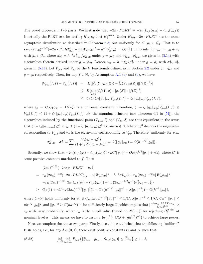
ASYMPTOTIC INFERENCE FOR SMOOTHING SPLINE 57
The proof proceeds in two parts. We first note that −2n · PLRT ′ ≡ −2n(`n,λ(gn0) − `n,λ(gn,λ))
is actually the PLRT test for testing H1n against Hglobal1 . Under H1n, −2n · PLRT ′ has the same
asymptotic distribution as described in Theorem 5.3, but uniformly for all gn ∈ Ga. That is to
say, (2un0)−1/2(−2n · PLRT ′n,λ − n‖Wλgn0‖2 − h−1σ2Kn0) = OP (1) uniformly for gn0 = g0 + gn
with gn ∈ Ga, where un0 = h−1σ4Kn0/ρ
2Kn0 under g = gn0 and σ2
Kn0, ρ2Kn0 are given in (5.14) with
eigenvalues therein derived under g = gn0. Denote un = h−1σ4K/ρ
2K under g = g0 with σ2
K , ρ2K
given in (5.14). Let Vgn0 and Vg0 be the V functionals defined as in Section 2.2 under g = gn0 and
g = g0 respectively. Then, for any f ∈ H, by Assumption A.1 (a) and (b), we have
|Vgn0(f, f)− Vg0(f, f)| = |E{[¨a(Y ; gn0(Z))− ¨a(Y ; g0(Z))]|f(Z)|2}|
≤ E{supa∈I|`′′′a (Y ; a)| · |gn(Z)| · |f(Z)|2}
≤ C0C1C2‖gn‖supVgn0(f, f) = ζ0‖gn‖supVgn0(f, f),
where ζ0 = C0C1C2 = 1/(2ζ) is a universal constant. Therefore, (1 − ζ0‖gn‖sup)Vgn0(f, f) ≤
Vg0(f, f) ≤ (1 + ζ0‖gn‖sup)Vgn0(f, f). By the mapping principle (see Theorem 6.1 in [54]), the
eigenvalues induced by the functional pairs (Vgn0 , J) and (Vg0 , J) are thus equivalent in the sense
that (1− ζ0‖gn‖sup)γn0ν ≤ γν ≤ (1 + ζ0‖gn‖sup)γn0
ν for any ν ∈ N, where γn0ν denotes the eigenvalue
corresponding to Vgn0 and γν is the eigenvalue corresponding to Vg0 . Therefore, uniformly for gn0,
σ2Kn0 − σ2
K =∑ν
hλ(γν − γn0ν )
(1 + λγn0ν )(1 + λγν)
= O(‖gn‖sup) = O(h−1/2‖gn‖).
Secondly, we show that −2n(`n,λ(g0)− `n,λ(gn0)) ≥ nC ′‖gn‖2 +OP (n1/2‖gn‖+ nλ), where C ′ is
some positive constant unrelated to f . Then
(2un)−1/2(−2nrK · PLRT − un)
= rK(2un)−1/2(−2n · PLRT ′n,λ − n‖Wλgn0‖2 − h−1σ2Kn0) + rK(2un)−1/2n‖Wλgn0‖2
−rK(2un)−1/2 · 2n(`n,λ(g0)− `n,λ(gn0)) + rK(2un)−1/2h−1(σ2Kn0 − σ2
K)
≥ OP (1) + nC ′rK(2un)−1/2‖gn‖2(1 +OP (n−1/2‖gn‖−1 + λ‖gn‖−2)) +O(h−1‖gn‖),
where OP (·) holds uniformly for gn ∈ Ga. Let n−1/2‖gn‖−1 ≤ 1/C, λ‖gn‖−2 ≤ 1/C, Ch−1‖gn‖ ≤
nh1/2‖gn‖2, and ‖gn‖2 ≥ C(nh1/2)−1 for sufficiently large C, which implies that |−2nrK ·PLRT−un(2un)1/2 | ≥
cα with large probability, where cα is the cutoff value (based on N(0, 1)) for rejecting Hglobal0 at
nominal level α . This means we have to assume ‖gn‖2 ≥ C(λ+ (nh1/2)−1) to achieve large power.
Next we complete the above two parts. Firstly, it can be established that the following “uniform”
FBR holds, i.e., for any δ ∈ (0, 1), there exist positive constants C and N such that
(S.52) infn≥N
infgn∈Ga
Pgn0
(‖gn,λ − gn0 − Sn,λ(gn0)‖ ≤ Can
)≥ 1− δ,

58 Z. SHANG AND G. CHENG
where an is defined in (3.5), The proof of (S.52) follows by a careful reexamination of Theorem 3.4.
Specifically, one can choose C and M (to be unrelated to gn ∈ Ga) to be large so that the event
Bn1 ∩Bn2, which is defined in the proof of Theorem 3.4, has probability greater than 1− δ4 . Then
by going through exactly the same proof, it can be shown that when n ≥ N for some suitably
selected N , for any gn ∈ Ga, (S.13) holds with probability greater than 1− δ/2 (by properly tuning
the probability), with the constant C ′ therein only depending on C,M, cm. By going through the
proofs of (S.14) and (S.15), it can be shown that for n ≥ N and gn ∈ Ga, with probability larger
than 1− δ, ‖gn,λ − gn0 − Sn,λ(gn0)‖ ≤ Can, where the constant C and N are unrelated to gn ∈ Ga.
Using (S.52) and by exactly the same proof of Theorem 5.3, it can be shown that −2n · PLRT ′
follows the same asymptotic normal distribution under H1n : g = gn0 as in Theorem 5.3, uniformly
for gn ∈ Ga.
For simplicity, denote Ri = `(Yi; g0(Zi))− `(Yi; gn0(Zi)) for i = 1, . . . , n. Then
(S.53) E{|n∑i=1
[Ri − E(Ri)]|2} ≤ nE{R2i } = nE{| − εign(Zi) + ¨
a(Yi; g∗n0(Zi))gn(Zi)
2|2},
where g∗n0(z) = g0(z) + t∗gn(z) for t∗ ∈ (0, 1), implying g∗n0(z) ∈ I0 for any z. By Assumption
A.1, we get that (S.53) is uniformly O(n‖gn‖2) over gn ∈ Ga. Therefore, uniformly over gn ∈ Ga,
n(`n,λ(g0)− `n,λ(gn0)− E{`n,λ(g0)− `n,λ(gn0)}) = OP (n1/2‖gn‖).
On the other hand, by supa∈I¨a(Y ; a) < 0, we can find C ′ > 0 (unrelated to gn ∈ Ga) such that
E{DSn,λ(g∗n0)gngn} = E{¨a(Y ; g∗n0(Z))|gn(Z)|2} − λJ(gn, gn) ≤ −C ′‖gn‖2/2. Therefore,
E{`n,λ(g0)− `n,λ(gn0)} = E{Sn,λ(gn0)(−gn) + (1/2)DSn,λ(g∗n0)gngn}
≤ λJ(gn0, gn)− C ′‖gn‖2/2 = O(λ)− C ′‖gn‖2/2,
where the last equality holds by J(gn, gn) ≤ M and |J(gn0, gn)| ≤ |J(g0, gn)| + J(gn, gn) ≤
J(g0, g0)1/2M1/2 + M . Consequently, 2n(`n,λ(g0)− `n,λ(gn0)) ≤ −nC ′‖gn‖2 + OP (nλ + n1/2‖gn‖).
This completes the proof.
S.18. Proof of Lemma 6.1. We need the following two inequalities to establishing (6.3):∫ ∞0
1
(1 + x2m)ldx =
∞∑k=0
∫ 2πh†(k+1)
2πh†k
1
(1 + x2m)ldx ≤
∞∑k=0
2πh†
(1 + (2πh†k)2m)l,
and by a similar argument,∫∞
01
(1+x2m)ldx ≥
∑∞k=1
2πh†
(1+(2πh†k)2m)l. This completes the proof.
University of Notre Dame
Notre Dame, IN 46545
Email: [email protected]
Department of Statistics
Purdue University
250 N. University Street
West Lafayette, IN 47906
Email: [email protected]
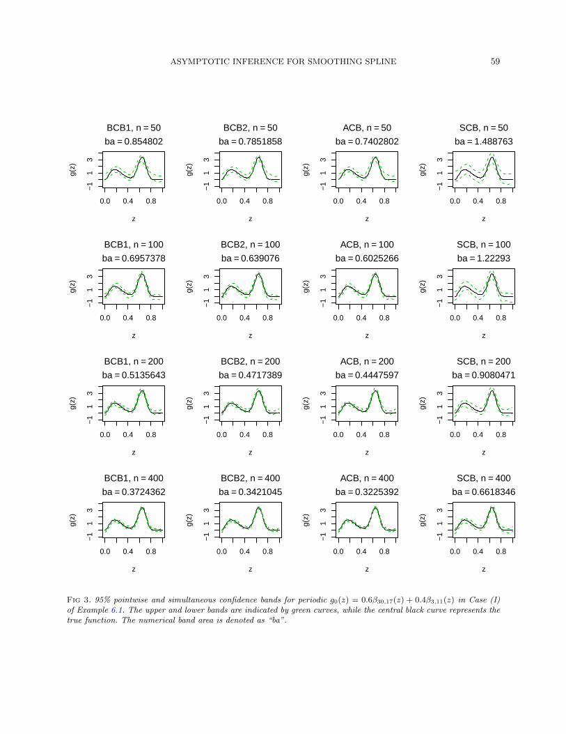
ASYMPTOTIC INFERENCE FOR SMOOTHING SPLINE 59
0.0 0.4 0.8
−1
13
z
g(z)
BCB1, n = 50
ba = 0.854802
0.0 0.4 0.8−
11
3
z
g(z)
BCB2, n = 50
ba = 0.7851858
0.0 0.4 0.8
−1
13
z
g(z)
ACB, n = 50
ba = 0.7402802
0.0 0.4 0.8
−1
13
z
g(z)
SCB, n = 50
ba = 1.488763
0.0 0.4 0.8
−1
13
z
g(z)
BCB1, n = 100
ba = 0.6957378
0.0 0.4 0.8
−1
13
z
g(z)
BCB2, n = 100
ba = 0.639076
0.0 0.4 0.8−
11
3
z
g(z)
ACB, n = 100
ba = 0.6025266
0.0 0.4 0.8
−1
13
z
g(z)
SCB, n = 100
ba = 1.22293
0.0 0.4 0.8
−1
13
z
g(z)
BCB1, n = 200
ba = 0.5135643
0.0 0.4 0.8
−1
13
z
g(z)
BCB2, n = 200
ba = 0.4717389
0.0 0.4 0.8
−1
13
z
g(z)
ACB, n = 200
ba = 0.4447597
0.0 0.4 0.8−
11
3
z
g(z)
SCB, n = 200
ba = 0.9080471
0.0 0.4 0.8
−1
13
z
g(z)
BCB1, n = 400
ba = 0.3724362
0.0 0.4 0.8
−1
13
z
g(z)
BCB2, n = 400
ba = 0.3421045
0.0 0.4 0.8
−1
13
z
g(z)
ACB, n = 400
ba = 0.3225392
0.0 0.4 0.8
−1
13
z
g(z)
SCB, n = 400
ba = 0.6618346
Fig 3. 95% pointwise and simultaneous confidence bands for periodic g0(z) = 0.6β30,17(z) + 0.4β3,11(z) in Case (I)of Example 6.1. The upper and lower bands are indicated by green curves, while the central black curve represents thetrue function. The numerical band area is denoted as “ba”.
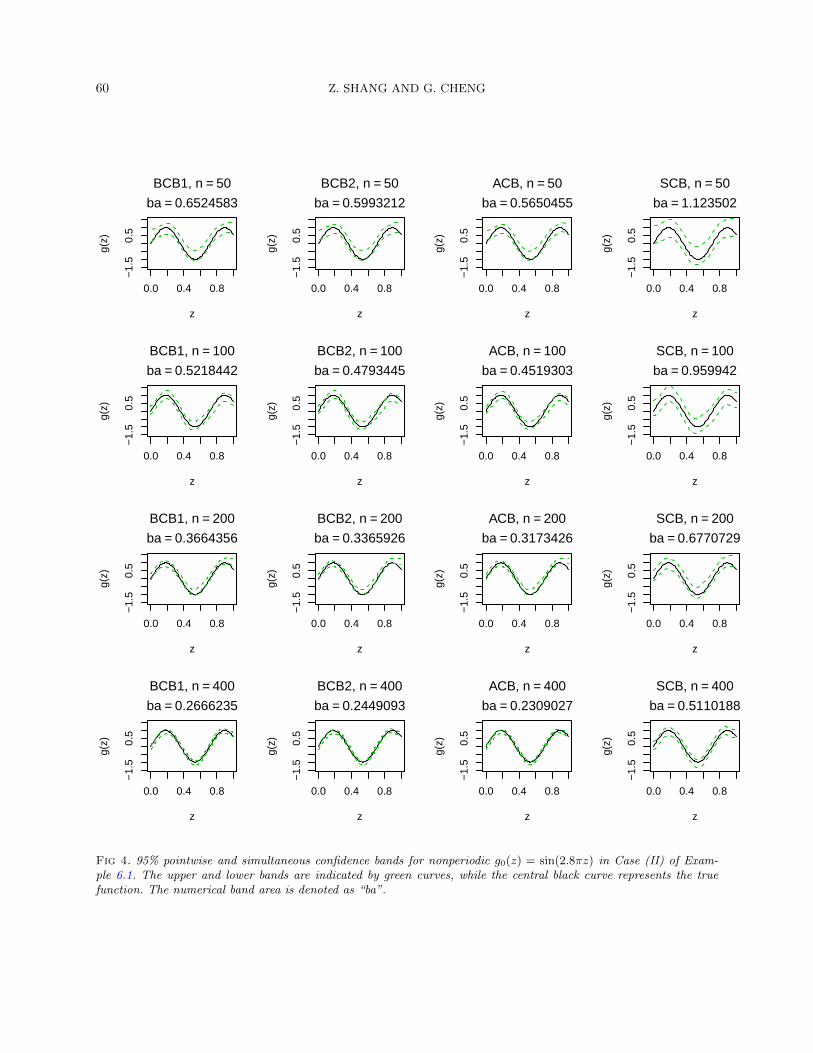
60 Z. SHANG AND G. CHENG
0.0 0.4 0.8
−1.
50.
5
z
g(z)
BCB1, n = 50
ba = 0.6524583
0.0 0.4 0.8−
1.5
0.5
z
g(z)
BCB2, n = 50
ba = 0.5993212
0.0 0.4 0.8
−1.
50.
5
z
g(z)
ACB, n = 50
ba = 0.5650455
0.0 0.4 0.8
−1.
50.
5
z
g(z)
SCB, n = 50
ba = 1.123502
0.0 0.4 0.8
−1.
50.
5
z
g(z)
BCB1, n = 100
ba = 0.5218442
0.0 0.4 0.8
−1.
50.
5
z
g(z)
BCB2, n = 100
ba = 0.4793445
0.0 0.4 0.8−
1.5
0.5
z
g(z)
ACB, n = 100
ba = 0.4519303
0.0 0.4 0.8
−1.
50.
5
z
g(z)
SCB, n = 100
ba = 0.959942
0.0 0.4 0.8
−1.
50.
5
z
g(z)
BCB1, n = 200
ba = 0.3664356
0.0 0.4 0.8
−1.
50.
5
z
g(z)
BCB2, n = 200
ba = 0.3365926
0.0 0.4 0.8
−1.
50.
5
z
g(z)
ACB, n = 200
ba = 0.3173426
0.0 0.4 0.8−
1.5
0.5
z
g(z)
SCB, n = 200
ba = 0.6770729
0.0 0.4 0.8
−1.
50.
5
z
g(z)
BCB1, n = 400
ba = 0.2666235
0.0 0.4 0.8
−1.
50.
5
z
g(z)
BCB2, n = 400
ba = 0.2449093
0.0 0.4 0.8
−1.
50.
5
z
g(z)
ACB, n = 400
ba = 0.2309027
0.0 0.4 0.8
−1.
50.
5
z
g(z)
SCB, n = 400
ba = 0.5110188
Fig 4. 95% pointwise and simultaneous confidence bands for nonperiodic g0(z) = sin(2.8πz) in Case (II) of Exam-ple 6.1. The upper and lower bands are indicated by green curves, while the central black curve represents the truefunction. The numerical band area is denoted as “ba”.