Loan Originations and Defaults in the Mortgage Crisis:

The Role of the Middle Class

Manuel Adelino

Duke University

Antoinette Schoar

MIT and NBER

Felipe Severino

Dartmouth College

Current version: February 2016; first version: November 2014

This paper highlights the importance of middle-class and high-FICO borrowers for the mortgage

crisis. Contrary to popular belief, which focuses on subprime and poor borrowers, we show that

mortgage originations increased for borrowers across all income levels and FICO scores. The

relation between mortgage growth and income growth at the individual level remained positive

throughout the pre-2007 period. Finally, middle-income, high-income, and prime borrowers all

sharply increased their share of delinquencies in the crisis. These results are consistent with a

demand-side view, where homebuyers and lenders bought into increasing house values and

borrowers defaulted after prices dropped. (JEL R30, D30, G21)

We thank Gene Amromin, Nittai Bergman, Markus Brunnermeier, Ing-Haw Cheng, Ken French,

Matthieu Gomez, Raj Iyer, Amir Kermani, Andrew Lo, Debbie Lucas, Sendhil Mullainathan,

Debarshi Nanda, Charles Nathanson, Christopher Palmer, Jonathan Parker, Adriano Rampini,

David Robinson, Steve Ross, Amit Seru, Andrei Shleifer, Jeremy Stein, Nancy Wallace, Jialan

Wang, Paul Willen, and seminar participants at AFA, Banco Central de Chile, Berkeley,

Brandeis, Cass, Columbia, CFPB Research Forum, Dartmouth, Duke, Econometric Society,

Federal Reserve Bank of New York, Federal Reserve Board, Harvard Business School, Imperial

College London, Macro Financial Modeling Conference, Maryland, McGill, MIT, NBER

Corporate Finance, NBER SI Capital Markets and the Economy, NBER SI Household Finance,

Princeton, and UNC for thoughtful comments. This paper was previously circulated under the

title “Changes in Buyer Composition and the Expansion of Credit during the Boom.” Send

correspondence to Antoinette Schoar, MIT Sloan School of Management 100 Main Street, E62-

638. Cambridge, MA; telephone: (617) 253-3763. E-mail: aschoar@mit.edu.

1

Understanding the origins of the housing crisis of 2007–2008 has been an ongoing challenge for

financial economists and policy makers alike. One predominant narrative to explain the crisis is

that changes in mortgage origination technology, coupled with incentives in the financial sector,

led to unprecedented lending to low-income and subprime (poor credit quality) borrowers,

causing house prices to accelerate and subsequently to crash. This narrative builds on a key

finding by Mian and Sufi (2009) that growth in mortgage credit for home purchases at the ZIP

code level became negatively correlated with per capita income growth in the run-up to the

financial crisis, suggesting that lending became decoupled from income, especially in areas with

strong house price growth. As a result, an emphasis has been placed on understanding what role

the financial industry played in providing credit at unsustainable levels, in particular to low-

income and subprime borrowers.1

In contrast, we provide new analysis of both the debt origination dynamics leading up to the

financial crisis and the patterns of default during the crisis that run counter to this narrative. Our

results point to an important role of middle-class and prime borrowers in the housing boom and

bust. First, we show that between 2002 and 2006 mortgage origination increased for borrowers

across the whole income distribution, not just for low-income or subprime borrowers. In line

with previous years, the majority of new mortgages by value were originated to middle-class and

high-income segments of the population even at the peak of the boom. Similarly, the share of

originations to subprime borrowers (those with a credit score below 660) relative to high credit

score borrowers remained stable across the pre-crisis period. Although the pace of origination

rose in low-income ZIP codes, this increase did not translate into significant changes in the

overall distribution of credit, given that it started from a low base (borrowers in low-income and

1 “The expansion of mortgage credit to marginal borrowers kicked off an explosion in household debt in the U.S.

between 2000 and 2007” (Mian and Sufi 2014).

2

subprime ZIP codes obtain fewer and significantly smaller mortgages on average).2

Second, delinquency patterns highlight the importance of middle-income and prime

borrowers. We show that the share of mortgage dollars in delinquency stemming from the lowest

income groups decreased during the financial crisis. In contrast, middle- and high-income

borrowers constituted a larger share of mortgage dollars in delinquency than in any prior year.

The magnitudes are large: for the 2003 mortgage cohort, the top quintile of the income

distribution constituted only 13% of mortgage dollars in delinquency three years later, whereas

for the 2006 cohort, the top income quintile made up 23% of the delinquencies three years out. In

contrast, over the same period, the contribution to delinquencies from the ZIP codes in the lowest

20% of the income distribution fell from 22% to only 11%.3

We find a similar pattern when we look at credit scores: the share of mortgage defaults from

borrowers with high credit scores increased during the crisis, whereas the share for subprime

borrowers dropped. When we compare cohorts of loans originated from 2003 to 2006 and track

defaults three years later, we see that the fraction of mortgage dollars that are in delinquency

from high credit score borrowers (those with a FICO score above 720) goes from 9% for the

2003 cohort to 23% of delinquencies for the 2006 cohort. The share of delinquencies from

borrowers below a credit score of 660 dropped from 71% in the 2003 mortgage cohort to 39%

for the 2006 cohort.4

The increase in the contribution by prime borrowers to overall

delinquencies is particularly concentrated in the 50% of ZIP codes that saw the steepest run-up in

2 The average purchase mortgage for borrowers in the lowest income quartile of ZIP codes was about $97k as of

2002, and approximately two mortgages were originated per 100 residents per year. Borrowers in the top quartile of

ZIP codes obtain average mortgages of over $246k, and about three mortgages per 100 residents. 3 In this article we look at origination and delinquency patterns by income and credit score, but we are not making

welfare statements. Although lower-income borrowers saw a reduction in their contribution to aggregate

delinquency, it is likely that lower-income households (and ZIP codes) suffered more from defaults than higher

income ones. This might be driven by more limited nonhousing wealth, worse income shocks, or lack of other

funding possibilities. 4 A FICO score of 660 is a common cutoff for subprime borrowers (see, for example, Mian and Sufi 2009).

3

prices pre-2007 and a sharp drop thereafter.5

These results describe aggregate origination and delinquency by income and credit score

groups, but we also show that, even at the micro level, credit growth did not decouple from

income growth, as proposed by Mian and Sufi (2009). This earlier evidence relied on a

regression of growth in total dollar value of mortgage originations at the ZIP code level on the

growth in average household income from the Internal Revenue Service (IRS). The growth in

ZIP-code-level mortgage originations, however, combines increases at the intensive margin

(changes in average mortgage size) with the extensive margin (growth in the number of

mortgages originated in a ZIP code). Given that households, not ZIP codes, take on mortgages,

only the relation between individual mortgage size and income can inform us about changes in

the debt burden across households.

We find that the negative correlation of income and purchase mortgage credit is driven

entirely by a change in the velocity of mortgage origination (the number of mortgages originated

in a ZIP code in a given year), not by decoupling the growth in average mortgage size from

income growth. In fact, growth in individual mortgage size is strongly positively related to the

growth in IRS household income throughout the precrisis period. The apparent decoupling of

ZIP-code-level credit growth and per capita income growth is due solely to the negative relation

between the number of new originations and per capita income growth. This negative correlation

is concentrated in high-income ZIP codes that saw fast per capita income growth and moderate

growth in the number of mortgages during this period. For the bottom 75% of ZIP codes, the

relation between growth in dollar volume of originations and per capita income growth is always

5 It is important to emphasize that this paper classifies borrowers based on income and credit scores, which is

distinct from categorizations based on loan characteristics. Although classifications of loans as prime or subprime

may be interesting and important in their own right, we focus on investigating potential distortions along the

distribution of borrowers.

4

positive.

In addition, the relation between mortgage growth and household income is negative only

when county fixed effects are included in the regression, as proposed by Mian and Sufi (2009).

However, this specification employs only within-county variation and abstracts from any cross-

county variation. Given that there is significant variation in the incidence of the credit boom

across counties in the United States, we argue that it is important to include both between- and

within-county variation in the data. Removing the county fixed effects from the regression yields

a positive relation between credit growth and income growth, as the between-county coefficients

are strongly positive.

To be in line with prior literature, we have so far measured household income using IRS

income at the ZIP code level. But this income measure might be affected by composition effects,

since it combines the income of new home buyers and the income of the existing stock of

residents in an area. At any point in time buyers in an area have approximately double the

income of the average resident. We show that this is true both before the 2000s and during the

height of the credit expansion. To eliminate this potential composition effect, we repeat the

analysis with individual buyer income from the Home Mortgage Disclosure Act (HMDA). We

find that both total mortgage credit and average mortgage size are positively related to growth in

buyer income. In addition, when we look at a longer period, between 1996 and 2007, we confirm

that there is neither a reversal of the sign nor a change in the slope between credit flows and

income growth using individual borrower income.

To alleviate any concern that overstatement of reported income might be driving the results

5

using borrower income, we conduct a series of robustness tests.6 First, we repeat our analysis

separately for ZIP codes with more versus fewer agency loans (those purchased by one of the

government-sponsored enterprises, or GSEs) and show that the results are unchanged. Because

GSE loans adhere to much stricter underwriting standards even during the boom period,

overstatement is a smaller concern for the sample of ZIP codes in which GSEs are more

prevalent. Second, we separate the data by areas with high and low origination shares by

subprime lenders, which again proxies for the propensity to misreport income, and obtain the

same result.7 We are, of course, not arguing that income misreporting did not occur during the

run-up to the crisis but simply that it does not explain the patterns we show here. We provide a

detailed discussion of why income overstatement does not drive the results in Adelino, Schoar,

and Severino (2015).

A related question is whether other forms of housing leverage, such as cash-out refinancing

and home equity credit lines, show the same trends that we document for purchase mortgages.

We show that the origination of cash-out refinances and second-lien loans are concentrated

among middle-class and upper-middle-class borrowers during this period. The results of the

relation between growth in purchase mortgages and growth in income are also largely unchanged

when we consider only refinancing transactions from the HMDA mortgage data set, as well as

data from Lender Processing Services (LPS) on cash-out refinances. These results confirm that

the expansion of credit across the income distribution is consistent for all mortgage products.

6 A number of recent studies show that misreporting borrower characteristics increased during the precrisis period

(see, e.g., Jiang, Nelson, and Vytlacil 2014; Ambrose, Conklin, and Yoshida 2015). 7 In addition, the magnitudes of overstatement documented in the literature are too small to explain our results.

Jiang, Nelson, and Vytlacil (2014) show that income was overstated by 20% to 25% for low documentation or no

documentation loans, themselves a small fraction of loans originated in this period (about 30%). Ambrose, Conklin,

and Yoshida (2015) estimate an 11% mean overstatement in the sample of borrowers most likely to exaggerate

income. However, the difference in buyer income and ZIP code household income is more than 75% even at the

beginning of the boom.

6

In sum, these results provide a new picture of the mortgage expansion before 2007 and

suggest that cross-sectional distortions in the allocation of credit did not drive the run-up in

mortgage markets and the subsequent default crisis. In contrast, our results point to an

explanation in which house price increases and drops played a central role during the credit

expansion and in subsequent defaults. We show that these areas saw a particularly strong

increase in delinquencies from middle- and high-income and credit score borrowers. A number

of prior papers have shown that credit rose significantly more in areas with high rates of house

price appreciation from 2002 to 2006, particularly through second liens and cash-out refinancing

(consistent with Hurst and Stafford 2004; Lehnert 2004; Campbell and Cocco 2007; Bostic,

Gabriel, and Painter 2009; Mian and Sufi 2011; Brown, Stein, and Zafar 2013). In addition, the

role of house prices in driving defaults is shown in Foote, Gerardi, and Willen 2008; Haughwout,

Peach, and Tracy 2008; Mayer, Pence, and Sherlund 2009; Palmer 2014; Ferreira and Gyourko

2015).

We also show that areas with high house price growth saw a significant increase in flipped

properties—that is, an increase in the velocity with which properties turned over. This increase in

the number of transactions as a response to increased house prices means that a larger fraction of

households held recently originated mortgages and thus were near or at their maximum leverage

level.

It is beyond the scope of this paper to analyze the drivers of house price dynamics. As Rajan

(2010) argues, the cumulative effect of low interest rates over the decade leading up to the

housing boom may have increased house prices through lowering user costs and increased

demand for credit (Himmelberg, Mayer, and Sinai 2005; Bernanke 2007). At the same time,

extrapolative expectations may have played a role in driving up house prices. Among many

7

others, Foote, Gerardi, and Willen (2012), Cheng, Raina, and Xiong (2014), Shiller (2014), and

Glaser and Nathanson (2015) argue that buyers as well as investors in the mortgage market held

highly optimistic beliefs about house price growth. Haughwout, Tracy, and van der Klaauw

(2011), Chinco and Mayer (2016), and Bhutta (2015) emphasize the role of investors in the

boom and bust. Coleman, LaCour-Little, and Vandell (2008) argue that subprime lending may

have been a joint product rather than the cause of the increase in house prices.8 Several papers on

the consequences of mortgage securitization focus on the expansion of credit to risky or marginal

borrowers (Nadauld and Sherlund 2009; Loutskina and Strahan 2009; Keys et al. 2010;

Demyanyk and Van Hemert 2011; Dell’Ariccia, Igan, and Laeven 2012; Agarwal et al. 2014;

Landvoigt, Piazzesi, and Schneider 2015). Our focus complements this literature, since we

analyze both how credit expanded along the whole distribution of borrowers and who

contributed most significantly to aggregate defaults. It is also possible that defaults by subprime

or low-income borrowers had contagion effects on middle-income and middle credit score

borrowers, but our paper shows that the mechanism underlying the crisis was not simply one of

cross-sectional distortions in the supply of credit to low-income and subprime borrowers.

Only a proper diagnosis of the credit crisis will allow for a meaningful response to prevent

similar events in the future. Many earlier explanations focused predominantly on supply-side

distortions in lending to the poor. These studies mainly propose microprudential regulation, such

as changing borrower screening processes or excluding certain borrower groups from credit

altogether, in particular low-income borrowers. Our results point to a need for macroprudential

regulation to prevent the systemic buildup of debt across households and to ensure that the

8 Glaeser, Gottlieb, and Gyourko (2010) also argue that easier access to credit cannot explain the increase in house

prices during the boom. Similarly, Adelino, Schoar, and Severino (2014) find a modest elasticity of house prices to

interest rates during the 1998–2005 period. In contrast, Kermani (2012), Corbae and Quintin (2015), and Di Maggio

and Kermani (2014) argue that looser credit standards helped feed the boom in housing prices and led to the

subsequent bust.

8

financial system has sufficient slack to guard against systemic shocks that are not tied to

individual borrower characteristics. It also points toward a central role of the financial sector: if

the buildup of systemic risk can have widespread economic impact, macroprudential regulation

ultimately has to trade off how much to restrict lending ex ante to minimize potential losses

versus how to assign ex post who bears the losses in case of a crisis.

1. Data Description

The analysis in this paper uses data from three primary sources: the Home Mortgage Disclosure

Act (HMDA) mortgage data set, income data from the Internal Revenue Service (IRS) at the ZIP

code level, and a 5% random sample of all loans in the Lender Processing Services data (LPS,

formerly known as McDash). The HMDA data set contains the universe of U.S. mortgage

applications in each year. The variables of interest for our purposes are the loan amount, the

applicant’s income, the purpose of the loan (purchase, refinance, or remodel), the action type

(granted or denied), the lender identifier, the location of the borrower (state, county, and census

tract), and the year of origination. We match census tracts from HMDA to ZIP codes using the

Missouri Census Data Center bridge. This is a many-to-many match, and we rely on population

weights to assign tracts to ZIP codes.9 We drop ZIP codes for which census tracts in HMDA

cover less than 80% of a ZIP code’s population.10

With this restriction, we arrive at 27,385

individual ZIP codes in the data.

IRS income data are obtained directly from the IRS, and we use the adjusted gross income of

households that filed their taxes in a particular year in that ZIP code. IRS data are not available

9 In other words, ZIP codes often have more than one census tract associated with them, and census tracts can

overlap with more than one ZIP code. The Missouri Census Data Center bridges of tracts to ZIP codes using

population weights are obtained from http://mcdc.missouri.edu/websas/geocorr90.shtml for the 1990 definitions of

tracts (used in the HMDA data up to 2002) and http://mcdc2.missouri.edu/websas/geocorr2k.html for 2000 tract

definitions (used in the HMDA data starting in 2003). 10

This restriction drops 180 ZIP codes out of 23,565.

9

for 2003, so we exclude 2003 whenever we run panel regressions. In addition to total income and

per capita income, we use the number of tax filings in a ZIP code to construct an estimate of the

population in a ZIP code in each year.11

We obtain house price indexes from Zillow.12

The ZIP-

code-level house prices are estimated using the median house price for all homes in a ZIP code

as of June of each year. Zillow house prices are available for only 8,619 ZIP codes in the HMDA

sample for this period, representing approximately 77% of the total mortgage origination volume

in HMDA.13

We also use a loan-level data set from LPS that contains detailed information on the loan and

borrower characteristics for both purchase mortgages and mortgages used to refinance existing

debt. This data set is provided by the mortgage servicers, and we have access to a 5% sample of

the data. The LPS data include not only loan characteristics at origination but also the

performance of loans after origination, allowing us to look at ex post delinquency and defaults.

One constraint of using the LPS data is that coverage improves over time, so we start the analysis

in 2003 when we use this data set. Coverage of the prime market by the LPS data is relatively

stable at 60% during this period, but its coverage of the subprime market is lower (at around

30%) at the beginning of the sample and improves to close to 50% at the end of the sample

(Amromin and Paulson 2009).

Given the somewhat limited coverage of the subprime market in the LPS data, in particular

11

IRS ZIP code information is available at www.irs.gov/uac/SOI-Tax-Stats-Individual-Income-Tax-Statistics-ZIP-

Code-Data-(SOI). Data are available on the Web site for 1998, 2001, and 2004 onward, and we obtained the 2002

data on a CD from the IRS directly. The ZIP code population is approximated by multiplying the number of

exemptions by a factor of 0.9 (this factor is obtained based on 2008 population estimates constructed by adding the

number of returns, the number of returns filing jointly, and the number of dependents). 12

Zillow house prices are available at www.zillow.com/research/data/. 13

Mian and Sufi (2009) use a sample of 3,014 ZIP codes with available Fiserv Case Shiller Weiss house price data

at the ZIP code level covering 30% of U.S. households and 45% of U.S. mortgage debt (according to the Online

Appendix to the paper). We provide a longer discussion of the sample of ZIP codes used in this paper, as well as

results using the whole HMDA data set, in Section IA.1 of the Internet Appendix.

10

with respect to loans included in private-label mortgage-backed securities, we also use data from

Blackbox Logic and Freddie Mac (a random sample of 50,000 loans per year from the single-

family loan data set) on mortgage originations and delinquencies. The Blackbox Logic data

include approximately 90% of privately securitized loans in the 2002–2006 period, so they

include almost the whole population of subprime loans that were privately securitized (as well as

Alt-A and “jumbo prime” loans). The public Freddie Mac data, on the other hand, include

higher-quality loans that were included in Freddie Mac securities and had to conform to agency

guidelines.

To identify subprime loans, we rely on the subprime and manufactured home lender list

constructed by the Department of Housing and Urban Development (HUD) for the years

between 1993 and 2005. This list includes lenders that specialize in these loan types and are

identified by a combination of features, such as the average origination rate, the proportion of

loans for refinancing, and the share of loans sold to Fannie Mae or Freddie Mac, among others.14

The data contain lender names, agency codes, and lender identification numbers, and we use

these identifiers to match this list to HMDA.

Last, we use household income and debt data from the 2001, 2004, and 2007 waves of the

Federal Reserve Board Survey of Consumer Finances (SCF). The SCF is a household survey that

asks consumers for detailed information about their finances and savings behavior and is

conducted every three years as a repeated cross-section. We use these data to construct a debt-to-

income (DTI) measure that includes all mortgage-related debt and to ask where along the income

distribution we observe an increase in DTI levels.

14

The complete list, as well as the detailed criteria for inclusion of lenders in the list, is available at

www.huduser.org/portal/datasets/manu.html. Mayer and Pence (2009) discuss advantages and disadvantages of

using this list to identify subprime loans.

11

2. Summary Statistics

Table 1 presents the descriptive statistics for the main variables in our sample. We report

averages and standard deviations for the full sample and broken down by household income from

the IRS as of 2002 (Columns 2–4) and by the level of house price growth (Columns 5–7). The

sample is based on the 8,619 ZIP codes that have nonmissing house price data at the ZIP code

level from Zillow. Table IA.1 of the Internet Appendix shows summary statistics for all ZIP

codes in HMDA.

The first two rows show the ZIP code IRS-adjusted gross income per capita as of 2002, as

well as home buyer income from HMDA as of 2002 (that is, at the beginning of the boom

period). When we compare IRS income to HMDA income as of 2002, we see that the average

HMDA income of home buyers is 80% higher than the average household income reported to the

IRS. For the ZIP codes with the highest household income (Column 2), home buyers report

about 1.7 times the average IRS income in those ZIP codes, and home buyers in the lowest

income group report more than twice the average IRS income. This shows that, even before the

boom, there is a significant discrepancy between the average household income and the income

of home buyers.

Original mortgage balances are strongly increasing in the average ZIP code income.

Mortgages in the highest income quartile are, on average, 2.5 times larger than those in the

lowest income ZIP codes. Larger mortgages, along with more mortgages originated per resident

(50% more in the highest quartile than in the lowest one), mean that overall origination is heavily

concentrated in high- and middle-income ZIP codes (we consider shares of total origination in

more detail in the next section). The last three columns of panel A of Table 1 show that the ZIP

codes that experienced the biggest house price run-ups between 2002 and 2006 had higher

12

average buyer income and larger mortgage balances even as of 2002, especially when compared

to ZIP codes with small subsequent house price increases.

The main set of regressions in Section 4 focuses on the relation between growth in mortgage

origination and growth in ZIP code income. The (annualized) nominal growth rate of IRS

household income between 2002 and 2006 is 6.4% for the highest income ZIP codes and 3.5%

for the lowest income ones, consistent with expanding income inequality in the United States

during this period. Growth in home buyer income from HMDA is relatively similar across

household income quartiles (around 6%–7%).

The growth rate of total origination of purchase mortgages is 12% on average, but it varies

inversely with income level. Growth in total origination is about 8% in the ZIP codes in the

highest income quartile, and it is double this amount for the lowest quartile. However, the growth

rate in total origination combines growth in average mortgage balance and growth in the number

of mortgages. The difference in total mortgage growth across high- and low-income ZIP codes is

driven almost exclusively by differential growth rates in the number of mortgages originated (1%

in the highest income ZIP codes versus 10% in the lowest), rather than by differential growth in

average mortgage sizes.15

Panel B of Table 1 shows descriptive statistics for the 5% sample of

the LPS data set. The average mortgage balance at origination for the 2003 mortgage cohort is

slightly above the number for the whole HMDA data set.16

The average credit score in the data is

711, and average scores are increasing in ZIP code household income, as expected. The average

delinquency rate in the 2003 mortgage cohort is 3.7%, with a rate of 1.5% in the high-income

15

This increase in the number of purchase mortgages originated can be the result of new homeowners moving into

these areas (as in Guerrieri, Hartley, and Hurst 2013) or of more transactions by existing residents (home

“flipping”). 16

If we take into account an average growth rate of about 7% over 2002–2003, the discrepancy is about $23k

between the two data sets.

13

ZIP codes and 7% in the bottom quartile. A mortgage is defined as being delinquent if payments

become ninety days or more past due (i.e., 90 days, 120 days, or more in foreclosure or real

estate owned, REO) at any point during the three years after origination. Delinquency rates are

significantly higher for the 2006 cohort, at 18%, and they are once more monotonically

decreasing in income. Importantly, the proportional increase in default rates is much larger for

the top income ZIP codes than for the bottom ones, meaning that the fractions of overall

delinquencies shift toward the high-income bucket. We return to this issue in the next section.

3. Origination and Delinquency by Borrower Type and Cohort

We now consider how the flow of mortgage origination and the share of overall delinquent debt

changed across both the income and the credit score distributions. If, indeed, credit decoupled

from income and started flowing disproportionately to poorer households, we would expect to

see an increase in the share of credit originated to low-income and subprime home buyers. The

contribution of each income and credit score group to the aggregate origination patterns is

informative if we care about the impacts of changes in origination technology on the economy as

a whole. We use individual transaction-level data from HMDA, origination and delinquency data

from LPS, and income data from both the IRS (average ZIP-code-level household income) and

HMDA (buyer income). We restrict the sample to ZIP codes with nonmissing Zillow house price

data, about 77% of total purchase mortgage volume in HMDA.

3.1 Aggregate origination

We start by analyzing how aggregate mortgage origination changed across the income

distribution between 2002 and 2006. In panel A of Figure 1 we break out the dollar volume of

mortgages originated for home purchase in each year by the quintile that each borrower falls into

14

based on buyer income reported on each application. We sum the mortgage amounts originated

to all the households within an income quintile and divide this number by the amount of

mortgage debt originated in the United States in a given year.17

This picture highlights that

middle-class and richer borrowers obtained the majority of credit in all years during the boom

and that the proportion of mortgages originated by group holds steady between 2002 and 2006.

We see that the top quintile has a stable share of 34% in the value of mortgage originations in

2002, rising to 36% in 2006. Similarly, the bottom quintile accounts for about 11% of mortgage

dollars originated in both 2002 and 2006, meaning that purchase mortgage credit was allocated

similarly at the peak of the boom and at the beginning of the 2000s. Although the amount of

purchase mortgage originations increased in absolute value over this period, the distribution of

credit between poorer and richer households remained steady, with most credit going to the

richer segments of the population.18

The picture using IRS household income as of 2002 to form

quintiles (shown in Figure 1, panel B) also shows a largely stable pattern. Using the IRS income

thresholds, we see a drop from 35% to 30% for the top quintile, and this drop is compensated by

a 1% to 2% increase for the three lowest quintiles.19

Although this represents a significant

proportional change in total origination for some quintiles (particularly the lowest one), the

overall distribution looks similar over time, and the middle and the top quintiles still make up the

majority of originations even at the peak of the boom. Figure IA.1 of the Internet Appendix

shows that poorer households are significantly more leveraged than richer ones across all years

17

As of 2002, the buyer income cutoff for the bottom quintile is $41k, the second quintile corresponds to $58k, the

third quintile corresponds to $78k, and the fourth quintile corresponds to $112k. Figure IA.2 of the Internet

Appendix shows origination based on resorting ZIP codes using each year’s income per capita, rather than fixing

ZIP codes as of 2002. The shares in each bin are very similar to those in panel B of Figure 1. 18

Total purchase mortgage originations in the sample rise from $573 billion in 2002 to $887 billion in 2006 for our

sample of ZIP codes. 19

For this panel and all other figures using quintiles of IRS income, the cutoffs are as follows: the bottom quintile

cutoff corresponds to an average household income in the ZIP code as of 2002 of $34k, for Q2 it is $40k, for Q3 it is

$48k, and for Q4 it is $61k.

15

but that DTI levels measured in HMDA do not increase differentially for low-income borrowers

relative to high-income ones.20

Figure 2 divides originations by bins of FICO scores. This gives us another dimension by

which to determine whether marginal borrowers disproportionally increased their share of

originations during the boom. We define subprime borrowers as those below a cutoff of 660, the

typical FICO cutoff for subprime borrowers in the literature.21

We also include a second cutoff of

720, which is approximately the median credit score in the LPS sample.22

Panel A of Figure 2 shows that purchase mortgage originations across credit scores remained

stable during the boom period, very much in line with the findings regarding income. Just over

half of the origination volume goes to borrowers above 720 in all years, about 28%–30% goes to

borrowers with credit scores between 660 and 720, and only 17%–18% of mortgages go to

borrowers with credit scores below 660. This pattern stays unchanged from 2003 to 2006,

confirming that there was no disproportional increase in the share of credit going to subprime

borrowers.

As we point out in the data description, one concern with the LPS data is that they

underrepresent the low credit score (subprime) segment of the market, especially at the

beginning of the period, and this may influence some of the patterns we observe. To mitigate

concerns related to data representativeness, we replicate the analysis using data from Blackbox

Logic (a data set of privately securitized loans) in panel B. The figure confirms that purchase

20

Panel B of Figure A1 shows a DTI measure typically used in the industry (a measure of recurring mortgage

payments divided by monthly borrower income). The increase in DTI using this measure is relatively modest, and

again, borrowers at all income levels move in lockstep. 21

This is the cutoff used by the Federal Reserve Board (FRB), the Office of the Comptroller of the Currency (OCC),

the Federal Deposit Insurance Corporation (FDIC), and the Office of Thrift Supervision (OTS), and research papers,

such as Mian and Sufi (2009) and Demyanyk and Van Hemert (2011), among others. See also

www.fdic.gov/news/news/press/2001/pr0901a.html for a press release describing the guidelines for the FRB, OCC,

FDIC, and OTS. 22

The median scores in LPS are 721 in 2003, 716 in 2004, 718 in 2005, and 715 in 2006.

16

mortgage originations by credit score remained stable throughout this period.

3.1.1 Other Mortgage-Related Debt. The results so far have focused on purchase mortgages,

since these make up the majority of mortgage debt in the United States. However, it is possible

that other types of mortgage debt, such as refinancing mortgages or home equity loans, were

distributed very differently than purchase mortgages. In Figure 3 we use LPS data in 2006 to

compare the distribution of different loan products, namely, purchase mortgages, cash-out

refinance loans, rate refinance loans, and second liens. We focus on 2006 to ensure good

coverage of all products in LPS, and we split ZIP codes by average household income from the

IRS as of 2002.

Figure 3 shows that the distribution of all mortgage types is concentrated in the high-income

quintiles, similar to purchase mortgages. Cash-out refinances and second liens are generally

more concentrated in the second quintile than the first (consistent with the evidence by credit

score in Figure IA.11 in the Internet Appendix); the distribution of rate-refinancing mortgages is

very close to that of purchase mortgages. Given that the majority of mortgages originated are

purchase mortgages or rate-refinancing mortgages (total origination is shown above the bars for

each product in the figure), the overall distribution of mortgage origination is very close to that

of the purchase mortgages we have focused on for Figures 1 and 2.

We use SCF data to document how different mortgage-related products contributed to the

increase in the average stock of mortgage debt across the income distribution.23

Figure 4 reports

23

We thank Matthieu Gomez for the suggestion to replicate our DTI analysis using SCF data.

17

average DTI for households with nonzero mortgage debt sorted by income quintiles.24

The figure

shows that lower-income groups have higher DTIs than high-income groups, confirming the

patterns in Figure IA.1. However, the change in DTI is homogeneous across quintiles. This

means that, consistent with all the origination figures, DTI ratios did not grow disproportionately

for low-income households relative to high-income ones.

3.2 Aggregate Delinquency

Next, we analyze the distribution of mortgage delinquency across the income distribution.

Much of the literature focuses on the fact that delinquency rates are higher for lower-quality and

lower-income borrowers, but this section shows a breakdown of the dollar volume of credit that

is past due by income level and cohort of loans. This allows us to consider not just how the

likelihood of default by group changed but also each group’s value-weighted share of credit at

origination.

Figure 5 shows shares of delinquency by cohort using LPS data. Panel A of Figure 5 shows

the fraction of delinquent mortgages by income quintile for each cohort of loans between 2003

and 2006.25

Mortgages are defined as being delinquent if they become seriously delinquent (90

days or more past due), are in foreclosure, or are real estate owned (REO) at any point during the

first three years of the life of the mortgage. This measure follows a common definition of default

used elsewhere in the literature (see, e.g., Demyanyk and Van Hemert 2011).

In panel A of Figure 5 we use buyer income from HMDA to sort ZIP codes into quintiles.

Because LPS does not report applicant income, we use the average applicant income at the ZIP

24

Debt includes all mortgage-related debt, including home equity loans (SCF items MRTHEL (Mortgage and Home

Equity Loan, Primary Residence) and RESDBT (Other residential debt)). We divide the total debt by household

annual income to obtain the DTI. 25

Figure IA.3 of the Internet Appendix shows that origination patterns in LPS are very close to those we obtain in

Figure 1 with HMDA data.

18

code level from HMDA as of the beginning of the sample and merge it to LPS.26

Using HMDA

buyer income as of 2002 to sort ZIP codes, we see a pronounced increase in the share of

mortgage dollars in default for the highest income ZIP codes relative to the lower quintiles. For

the 2003 cohort, only 13% of the mortgage value in delinquency within the first three years

comes from borrowers in the top income quintile, while 22%–23% comes from each of the three

lowest income quintiles. However, from 2003 to 2006 the middle and even the highest income

quintiles become much more important in default: for the cohort of loans originated in 2006,

49% of the value of delinquencies within three years comes from the two top income quintiles,

and only 29% comes from the lowest two.

In panel B of Figure 5 we break out the volume of delinquent mortgages by income quintiles

using IRS household income at the ZIP code level as of 2002. The patterns by cohort are in line

with those obtained sorting by the average buyer income (though somewhat less pronounced).

For example, the top income quintile rises from a share of 12% in 2003 cohort to 17% in 2006,

and the second highest income quintile increases from 21% to 24%. In contrast, we see that the

lower income quintiles constitute a smaller share than before: the lowest quintile drops from 22%

to 19%, and the second lowest declines from 23% to 19%.

Figure 6 analyzes delinquency patterns by borrower credit score. As discussed before, credit

scores give us another dimension to determine whether marginal and low-quality borrowers were

primarily responsible for driving up delinquencies in the crisis. As in the other panels, we find a

dramatic reversal in the share of delinquencies across high and low credit score groups from

loans originated in 2006 with respect to the 2003 cohort. Panel A shows the splits of borrowers

in the LPS data. The share of mortgage dollars in delinquency for borrowers with credit scores

26

Note that by fixing applicant income as of the beginning of the period, this analysis cannot be contaminated by

concerns of income misreporting during the mortgage boom.

19

above 720 grows from 9% to 23%. It also increases for the middle group (those between 720 and

660) from 20% to 38%. At the same time, we see a dramatic decline for the group below 660

(subprime borrowers), dropping from 71% to 39%. We obtain similar patterns in panel B for

securitized loans in the Blackbox Logic data (although, as we point out before, the levels are

different, given that these are a specific type of loan). The picture is essentially unchanged if we

restrict the analysis to mortgages foreclosure (Figure IA.4 in the Internet Appendix).27

This

means that higher FICO score borrowers do not have a visibly better chance of getting out of

delinquency, at least in the aggregate patterns.28

Overall, the results show that, although there was a large increase in the overall volume of

delinquencies with the crisis, this was associated not with a concentration of defaults in low-

income ZIP codes or borrowers but rather with an increase in the share of delinquencies coming

from borrowers in higher-income groups, where delinquencies are usually much less common.

3.3 Delinquencies, borrower characteristics, and house price growth

The increase in the share of defaults by high FICO and middle-class borrowers in the crisis

points to a systematic shift in the drivers of default. A number of papers have suggested the

central role of house prices in defaults (Foote, Gerardi, and Willen 2008; Haughwout, Peach, and

Tracy 2008; Mayer, Pence, and Sherlund 2009; Palmer 2014; Ferreira and Gyourko 2015, who

27

Figure IA.5 of the Internet Appendix shows similar results for the Freddie Mac data set. This data set focuses on

the “prime” segment of the market, because mortgages originated for the Freddie Mac securitized mortgage pools

must conform to stricter underwriting standards than those in the private-label market. Figure IA.6 shows the dollar

value (instead of shares) of the purchase mortgages in delinquency in each cohort. Figure IA.7 shows that default

patterns in the other mortgage loan types look largely similar to those for purchase mortgages. Finally, Figure IA.8

shows the shares of delinquencies as a function of outstanding mortgages as of the last quarter of each year (instead

of by cohort, as in all other figures). The message is the same as in all delinquency results. 28

Following our paper, Mian and Sufi (2015) replicate our analysis using credit bureau data and confirm these

results: the increase in mortgage debt (purchase mortgages, as well as all other mortgage-related debt) was broadly

shared among all borrowers up to the 80th percentile in credit scores. They also show a significant reduction in the

share of delinquencies coming from low credit score borrowers in the crisis relative to the earlier period. Please see

Adelino, Schoar, and Severino (2015) for a detailed discussion and comparison of the results in both papers.

20

emphasize the importance of negative equity).

Importantly, we can look within ZIP codes and ask which borrowers drive the change in

shares of delinquencies across areas with rapid and slow house price increases. Figure 7 shows

that low credit score borrowers make up the overwhelming majority of delinquencies for the

2003 cohort in all ZIP codes (that is, across all house price growth quartiles). For the 2006

mortgages cohort, 62% of defaults come from borrowers above the subprime threshold of 660,

and these defaults are heavily concentrated in the two quartiles of ZIP codes with the highest

house price growth in the previous period: 37% of defaults come from borrowers above 660 in

the highest quartile of house price growth, and 14% come from those in the second highest.

Figure IA.9 of the Internet Appendix shows a similar pattern for “subprime” ZIP codes.29

Although defaults are concentrated in subprime ZIP codes (59% of delinquent mortgage dollars

for the 2006 cohort are in the top quartile by subprime originations), the most dramatic increase

in the share of dollars in default is found in borrowers above the 660 threshold. Similarly, Figure

IA.10 shows evidence suggesting a greater role of strategic default: we show that the share of

delinquencies coming from borrowers with credit scores above 660 is significantly higher in

nonrecourse states, consistent with strategic default being easier in states in which lenders lack

recourse on other assets beyond the secured debt. Some of these states also experienced a large

boom and bust in house prices, which is consistent with strategic default and of course also with

other economic shocks driving defaults.

4. Microevidence: Mortgage Credit and Income Growth

The results in Section 3 focus on aggregate credit flows to show that between 2002 and 2006

29

ZIP codes are classified according to the proportion of lending by subprime borrowers as defined by the HUD

subprime lender list.

21

mortgage originations expanded across the income and credit score distributions and that the

share of dollars in delinquency increased most sharply for middle-class and higher credit score

borrowers once house prices dropped. However, even if aggregate credit flows were largely

stable, it is possible that these aggregate dynamics mask within-group distortions in the

allocation of credit. In particular, there could have been a decoupling of credit from income

growth at the individual level.

To address this issue, we revisit the evidence in Mian and Sufi (2009). Specifically, their

work relies on regressing the growth in total purchase mortgage origination at the ZIP code level

on the growth in IRS income per capita.30

Importantly, growth in mortgage origination is a

combination of growth in the average loan size (the intensive margin) and the growth in the

number of loans given out in a ZIP code (the extensive margin). The distinction between the

intensive and extensive margins is crucial to differentiating an increase in individual leverage

(changes in the average debt burden for households) from higher volume (or quicker churning)

of transactions in the housing market.

The starting point for our analysis is the same regression used by Mian and Sufi (2009):

,

where is the growth of three alternative mortgage origination variables: in

Columns 1–3 of Table 2 (panel A), we use the annualized growth in the dollar value of mortgage

credit originated for home purchase at the ZIP code level from 2002 to 2006. Columns 4–9

decompose the aggregate mortgage growth into growth in the average mortgage size (the

30

It is worth emphasizing that income growth and income levels are strongly positively correlated during this

period, so that the observation that credit grew more in areas with slow income growth is closely related to the

observation that high-income ZIP codes saw a relative reduction in their overall share in originations. As we saw

above, however, the reduction in the share of the top quintile was accompanied by small increases in all other

quintiles (using IRS income quintiles; Figure 1), and this change in allocations is small in the aggregate (at about 4–

5 percentage points in total).

22

intensive margin) and growth in the number of mortgages generated in a ZIP code (the extensive

margin). is the growth in income per capita from the IRS at the ZIP

code level between 2002 and 2006, and is county fixed effects. The sample includes all

ZIP codes with nonmissing house price data from Zillow, and all growth rates are annualized.

The first column of panel A in Table 2 estimates the relation between the growth in total

origination and income without including county fixed effects, that is, using the full cross-

sectional variation within and between counties. The aim is to test whether mortgage credit

across the country increased faster in ZIP codes with weakly growing or declining incomes. We

show that the coefficient on per capita income growth in this regression is strongly positive and

statistically significant. This means that, when we use all of the within- and between-county

variation in mortgage growth and income growth, there is no decoupling of total purchase

mortgage growth and income growth.

Column 2 of panel A repeats the same regression but includes county fixed effects as

proposed by Mian and Sufi (2009). By absorbing county means, the within-county regression

underweights ZIP codes in more homogenous counties. We find a negative and significant

coefficient (−0.182), which is comparable to the estimate in Mian and Sufi (2009) and means

that the value of mortgage originations at the ZIP code level dropped by 0.182% for every

percentage point increase in income per capita in a ZIP code relative to the county average. The

third column of panel A focuses on the between-county variation of income and mortgage

growth. We find a strongly positive and significant relation, which explains the positive

coefficient in Column 1 using the total variation.

Next, we decompose the dependent variable into the average mortgage size (the intensive

margin) and the number of loans originated in a ZIP code (the extensive margin). The results in

23

Columns 4–6 of panel A show that the relation between growth in average mortgage size and per

capita income is strongly positive both for the within-county and between-county estimators. For

example, average mortgage size grows by about 0.27% for every percentage point relative

increase in per capita income within a county. This means that the relation between individual

mortgage balance and income cannot explain the negative correlation found in the previous

specification.

In the last three columns of panel A we look at the growth in the number of purchase

mortgages originated in a given ZIP code (the extensive margin) as the dependent variable. The

specification in Column 7 again uses both the within- and between-county variation and finds

that the relation between growth in the number of mortgages and in IRS income is negative. The

decomposition in Columns 8 and 9 shows that the relation between counties is strongly positive,

whereas the within-county variation is negative. So the source of the negative correlation in

Column 2 stems from the fact that the pace of mortgage originations (and possibly home buying)

increased relatively more in ZIP codes in which per capita income was growing less quickly

relative to county averages. Not only does the variation between counties overturn the negative

within-county coefficient, but the negative (within-county) coefficient could reflect the fact that

households select into ZIP codes based on house prices and that increasing income is associated

with more zoning restrictions and higher house prices (and, consequently, larger mortgages, as

we see above). This would mean that, within counties, we see more transactions (and more total

credit) flowing into lower-income ZIP codes in which homes are more affordable.31

In panel B of Table 2 we report the within- and between-county standard deviations of the

31

Table IA.2 of the Internet Appendix shows similar results using the whole HMDA data set (although we do not

obtain a negative coefficient when we use county fixed effects and the total mortgage origination as a dependent

variable).

24

three mortgage growth measures used in the regressions, as well as the growth of income per

capita from the IRS. This decomposition shows that the between-county standard deviation for

all variables is of the same magnitude as the variation within counties. The message from these

summary statistics is that focusing solely on the within-county regressions above misses a

quantitatively important component of the overall variation.

4.1 Panel specification

Panel C of Table 2 implements a panel regression to estimate the relation in panel A, but it

makes use of yearly data. This specification allows us to assess whether the slope of the relation

between income and mortgage growth changed from 2002 to 2006. IRS data are not available for

2003, so this year is excluded from the regressions. Whereas the earlier regressions in panel A

showed that the relation between mortgage growth and income growth were positive in the

precrisis period, one might question whether they became flatter over time. We use the following

specification:

.

The independent variables are the logarithm of the average IRS income of households in a

ZIP code interacted with a full set of dummies for all years in the sample (denoted ); FEt is

year fixed effects, and FEi is ZIP code fixed effects. Including ZIP code fixed effects and

interactions of the variables of interest with year dummies allows us to test how the sensitivity of

mortgage levels to income levels changed over time within ZIP codes.

The coefficient on the IRS income is positive and significant in all specifications in panel C

and very similar in magnitude to the results in panel A. As before, we break out total mortgage

origination into the average mortgage size by ZIP code and year (Column 3) and the number of

25

mortgages in a given ZIP code and year (Column 5). The results confirm that average loan size is

strongly positively related to the IRS income of existing buyers in a ZIP code.

Column 2 shows that the interaction terms with the year dummies are negative and

significant in all years. This means that the relation between the growth in mortgage origination

and the growth in average household income from the IRS became flatter over time. However,

Columns 4 and 6 show that this happens because the number of new mortgages in an area

became progressively less correlated with household income over the run-up to the crisis, as we

show in the previous panel. In contrast, we see no flattening of the relation between the average

size of mortgages and income.

4.2 Individual-level mortgage origination regressions

Next, we use individual mortgage transactions as the most disaggregated level of data to estimate

the relation of mortgage debt to income at the individual level. This allows us to use even finer

geographic controls (at the census tract level) than before. To this end, in Table 3 we use the

following specification:

,

where i indicates an individual borrower. is a year fixed effect, and is a census

tract fixed effect, the finest geographic breakdown available in the HMDA data set. The

independent variable of interest is the logarithm of the average IRS income of households in that

tract.32

Including census tract fixed effects allows us to test how the sensitivity of mortgage

levels to income levels changed within census tracts over time.

32

Because we do not have data on the average household income by tract, we use the same ZIP-code-to-tract

population-weighted bridge as before (from the University of Missouri Census Data Center) to impute average tract

income based on ZIP code household income.

26

Table 3 shows that, consistent with the previous (ZIP-code-level) regressions, the

coefficients on census tract income are positive and significant, and the result is unchanged when

we replace county fixed effects with census tract fixed effects (Column 3). As in panel C of

Table 2, Columns 2 and 4 confirm that the sensitivity of mortgage size to average household

income does not change significantly during the years of the boom (especially when we use tract

fixed effects).

4.3 Cross-sectional heterogeneity by ZIP code income

In this section we consider whether the relation between mortgage growth and income growth

varies with the income level of a ZIP code. In Table 4 we explore how mortgage and income are

related within low-, middle-, and high-income ZIP codes by breaking out the data into quartiles

based on the average IRS household income in a ZIP code as of 2002. The analysis follows

exactly the within-county (Table 4, panel A) and pooled OLS estimators (Table 4, panel B) of

Table 2. Columns 1–3 of panel A show that the relation is not the same across the different ZIP

code income quartiles. Only the top quartile by income (Column 1) shows a negative but

insignificant coefficient on the measure of average IRS income growth (−0.191). For the lower

three income quartiles in Columns 2 and 3, we find a positive (but not always significant)

relation between mortgage and household income growth.

Columns 4–9 show that the relation between IRS household income and the average

mortgage size is strongly positive and significant, and the magnitude of the coefficient is

extremely stable across all income levels. In contrast, the negative correlation of the growth in

the number of mortgages and income is prominent only in the highest-income ZIP codes. For the

other three quartiles, we do not find a significant correlation between the number of mortgages

and ZIP code income growth. We repeat these regressions in panel B without county fixed

27

effects and find that these patterns are consistent and even stronger.

Taken together, we do not find evidence that home buyers in poorer ZIP codes were

changing their leverage disproportionally relative to income growth. In fact, the relation between

mortgage credit and borrower income is strongest for lower-income ZIP codes, which runs

against the idea that credit flowed disproportionately to poorer and marginal borrowers. The

relation between average household income and the number of mortgages originated in a ZIP

code is negative only for the ZIP codes with the highest income.

4.4 Buyer income versus IRS household income

To be consistent with prior literature, the specifications above use growth in IRS ZIP code

income per capita as the measure of income growth. However, as we already discuss, ZIP-code-

level income may mask differences between the income of home buyers and the income of the

average resident in a ZIP code. In fact, as we document in the descriptive statistics, home buyers

report substantially higher incomes than the average residents in a ZIP code (typically about

twice as high), even before the housing boom. In addition, a report by the Census Bureau shows

that more than 40% of home buyers move across counties on average, meaning that their income

growth is not captured by county- or ZIP-code-level IRS data.33

Given these facts, in Table 5 we consider the income of the people who buy a house (and

take out a purchase mortgage loan) in each ZIP code during a given year, as opposed to the

income of the average households. We use individual mortgage-level income data reported in

HMDA instead of IRS averages to measure the income growth of buyers, and we aggregate up to

33

J. P. Schachter, “Geographical mobility: 2002 to 2003,” Census Bureau, Current Population Reports, issued

March 2004. The report shows that from 2002–2003, about 7.4% of homeowners moved, of which 40% moved

across counties. Given that ZIP codes are much smaller geographic units than counties, we posit that an even larger

proportion of movers move across ZIP codes.

28

the ZIP code level by taking the average for each ZIP code. We follow exactly the specifications

in Table 2 and decompose the results into the growth in average mortgage size and in the number

of mortgages, as well as into the within- and between-county estimators.

The results in panel A confirm that there is a positive relation between the growth in total

credit originated for home purchase in a ZIP code and the growth in buyer income during the

housing boom, both with county fixed effects and when we consider the between-county

estimates. Columns 4–6 show that the growth in the average size of mortgages (the intensive

margin) is also strongly positively related to the income growth of borrowers in all

specifications. These results show that even when we use income data of home buyers from

HMDA (and thus there is no concern of misattributing heterogeneity between residents and

actual home buyers), there is no decoupling of mortgage growth from credit growth across the

income distribution.

4.4.1 Robustness to income misreporting. One concern in using borrower income is that

lenders or borrowers may have had an incentive to overstate income in the run-up to the crisis in

order to justify higher leverage. It is therefore important to mitigate the concern that changes in

income reporting (in HMDA) are the source of the strong relation between buyer income and

total mortgage growth shown in panel A of Table 5.34

Of course, this concern does not affect any

of the specifications using IRS income data shown in the previous sections.

This section does not serve to show that there was no income misreporting, which clearly

occurred during the run-up to the mortgage crisis. Several papers have shown that lenders

engaged in this behavior (see, e.g., Jiang, Nelson, and Vytlacil 2014; Ambrose, Conklin, and

34

There is also evidence of other forms of misreporting during this time, including the value of transactions (Ben-

David 2011) and mortgage quality in contractual disclosures in the secondary market (Piskorski, Seru, and Witkin

2015; Griffin and Maturana 2016).

29

Yoshida 2015). Rather, these tests rule out that income misreporting is responsible for the

relation between borrower income and mortgage growth found in panel A of Table 5.

Panel B of Table 5 breaks out the main sample into different quartiles based on the fraction

of mortgages originated and sold to Fannie Mae and Freddie Mac (the government-sponsored

enterprises, or GSEs) in the ZIP code, as well as the fraction of loans that were originated by

subprime lenders based on the subprime lender list constructed by the Department of Housing

and Urban Development (HUD; see Section 1 for details). Loans that were sold to (and then

guaranteed by) the GSEs had to conform to higher origination standards than those sold to other

entities and were thus less likely to have unverified applicant income.35

The idea in these tests is

to see whether ZIP codes with a lower fraction of loans sold to GSEs exhibit a stronger relation

between mortgage growth and buyer income. Similarly, loans originated by subprime lenders

were much more likely to have low or no documentation status, and if the correlations shown

above were driven by misreporting, we would expect the splits based on this fraction to generate

meaningful variation in the estimated coefficients.

For both measures of quality of origination, we do not find that coefficients on buyer income

vary significantly. The coefficient on buyer income growth is very similar in magnitude and

significance level across all quartiles of both the GSE origination fraction (Columns 1–3 of Table

5, panel B) and the fraction originated by subprime lenders (Columns 4–6).

We repeat our regressions of credit growth on buyer income growth for different periods

(Table 5, panel C). We consider four subperiods: 1996–1998, 1998–2002, 2002–2006, and

2007–2011. The coefficient from the regression of growth in total mortgage origination on buyer

35

Previous work, including Pinto (2010), has noted that origination standards for GSEs dropped between 2002 and

2006, but we find similar results when we split the sample by the fraction of loans originated by subprime lenders.

30

income growth is positive and significant for all periods and does not become flatter in the

precrisis years. The relation between average mortgage size growth and income growth is also

strongly positive and stable throughout all periods (Columns 4–6).

Taken together, the evidence in panels B and C suggests that the boom period does not

represent a “special” period in how mortgage credit growth tracked buyer income growth. There

is no evidence that income misreporting contaminates the findings with regard to the basic

relation we uncover.

4.5 Cash-out refinances and second liens

Parallel to the discussion in Section 3, the previous results on the relation between income and

mortgage growth focus on purchase mortgages. In this subsection we consider whether

refinancing mortgages show significantly different patterns in the precrisis period relative to

purchase mortgages and in particular whether refinancing debt flowed disproportionally to poor

households. In panel A of Table 6 we use the same specifications as in Table 2, but we now use

the growth in refinancing transactions (from HMDA) rather than in purchase mortgage

originations. We include all types of refinancing transactions because HMDA does not

distinguish between cash-out and rate refinancing transactions.

Growth in refinancing debt tracks income growth (the coefficient is positive and significant)

when we use a between-county estimator, and it is negative for the within-county estimator.

When we decompose ZIP-code-level mortgage growth into the average mortgage size and the

growth in the number of loans, the results are generally similar to those for purchase mortgages.

The estimated coefficient of average mortgage size on IRS income growth is positive and

significant without county fixed effects and in the between-county estimator, although it

approaches zero and is insignificant for the within-county estimator. Panel B of Table 6

31

implements a ZIP-code-level panel regression similar to the one in panel C of Table 2. The

relation between total refinancing mortgage growth and IRS income growth becomes

progressively flatter over time. But, as for purchase mortgages, almost all of the change in the

relation comes from the extensive margin (growth in the number of transactions). The relation

between growth in the average size of refinancing transactions and income growth is unchanged

over the period; that is, there is also no decoupling of individual mortgage size from income for

refinancing transactions.36

5. Conclusion

This paper shows that mortgage credit increased across all income levels and for prime and

subprime borrowers. As a result, even at the peak of the boom, high- and middle-income

borrowers accounted for the majority of credit originated in the mortgage market. At the same

time, there was no “decoupling” of mortgage credit growth and income growth at the micro level

during the period before the financial crisis. Once the crisis hit, high- and middle-income

borrowers, as well as borrowers with a credit score above 660, accounted for a much larger

fraction of mortgage dollars in delinquency relative to earlier periods, especially in areas in

which the crisis was preceded by more pronounced house price booms. Because these middle-

class borrowers held much larger mortgages, what looks like a small increase in their default

rates had a large impact on the aggregate stock of delinquent mortgages.

Although we show that mortgage sizes did not increase disproportionately for the poor and

subprime borrowers at origination, the stock of average household leverage increased across the

income distribution in the run-up to the financial crisis (see, among many examples, the quarterly

36

We also replicate these regressions using LPS loan-level data, where we can focus only on cash-out refinances

and confirm these results (see Table IA.3 in the Internet Appendix).

32

Federal Reserve Bank of New York’s Household Debt and Credit Report). This increase in the

stock of household mortgage debt was driven by two channels: the first was an increase in the

velocity of transactions. Households are typically at their highest DTI level when they buy a new

home, but most households then pay down their mortgage over time. If the velocity of house

sales and purchases goes up, a higher fraction of households have recent mortgages, and thus the

overall stock of debt in the economy goes up. Figure 8 below shows that the fraction of

properties sold twice within a year increased steeply over the boom. We also see that this trend

was prevalent across all ZIP codes, but it happened at a higher pace in ZIP codes that saw higher

house price increases during that time.

The second channel is that households releveraged via cash-out refinancing or other home

loan transactions. Parallel to a number of early studies, our data confirm that equity extractions

via cash-out refinancing or home equity lines increased strongly during the early 2000s. We

show that growth in refinancing debt was in line with income growth and that middle- and

higher-income groups had the largest share of overall originations, not just of purchase

mortgages.

Both of these channels rely on a rise in house values as a precursor to releveraging, rather

than on credit itself driving house prices. Combined with the fact that there were no significant

cross-sectional distortions in the allocation of credit in the boom, this suggests that demand-side

effects and possibly also expectations of future house prices increases could have been important

drivers in the mortgage expansion as borrowers and lenders bought into expected increases in

asset values.

Understanding the origins of the mortgage expansion and subsequent crisis is of key

importance in shaping policy recommendations proposed to guard against future crises. A view

33

that emphasizes only supply-side distortions and the role of unsustainable lending to low-income

borrowers argues primarily for a policy response of tight microprudential regulation on bank

lending standards, especially when lending to low-income borrowers. Following on this, some

scholars argue that the response to the crisis should have focused more aggressively on principal

debt forgiveness, since it would have funneled dollars only to those marginal households with a

high marginal propensity to consume. For example, Mian and Sufi call the lack of a widespread

principal reduction program “the biggest policy mistake of the Great Recession” (2014, 141). Of

course, given the costs involved in principal forgiveness, this solution would have been viable

only if a small fraction of homeowners, in particular the poor, were primarily responsible for

delinquencies in the crisis. Our findings show that this solution becomes very hard to justify

because the dollar amounts needed would have been unrealistically high (see also Eberly and

Krishnamurthy 2014, who compare the costs of these programs with those aimed at providing

liquidity to households, and the effects on consumption of both types of approaches), and the

ensuing moral hazard problems might have plagued mortgage markets for a long time.

Instead, our results highlight the importance of macroprudential regulation: if the buildup of

systemic risk can have widespread economic impact, effective regulation must ultimately trade

off how much to restrict lending upfront to minimize potential losses from the household sector

versus how to create slack in the financial system to make it more resilient to systemic shocks.

At the same time, more research and discussion is needed to determine how to assign who bears

the losses in times of crisis.

34

REFERENCES

Adelino, M., A. Schoar, and F. Severino. 2014. Credit supply and house prices: Evidence from

mortgage market segmentation. NBER Working Paper No. 17832.

———. 2015. Loan originations and defaults in the mortgage crisis: Further evidence. NBER

Working Paper No. 21320.

Agarwal, S., G. Amromin, I. Ben-David, S. Chomsisengphet, and D. D. Evanoff. 2014.

Predatory lending and the subprime crisis. Journal of Financial Economics 113:29–52.

Ambrose, B. W., J. Conklin, and J. Yoshida. 2015. Reputation and exaggeration: Adverse

selection and private information in the mortgage market. Working Paper, Penn State University.

Amromin, G., and A. L. Paulson. 2009. Comparing patterns of default among prime and

subprime mortgages. Economic Perspectives (Federal Reserve Bank of Chicago) 33.

Ben-David, I., 2011. Financial Constraints and Inflated Home Prices during the Real-Estate

Boom. American Economic Journal: Applied Economics 3:55–78.

Bernanke, B. S. 2007. Global imbalances: Recent developments and prospects. Bundesbank

Lecture, Berlin.

Bhutta, N. 2015. The ins and outs of mortgage debt during the housing boom and bust. Journal

of Monetary Economics 76:284–98.

Bostic, R., S. Gabriel, and G. Painter. 2009. Housing wealth, financial wealth, and consumption:

New evidence from micro data. Regional Science and Urban Economics 39:79–89.

Brown, M., S. Stein, and B. Zafar. 2015. The impact of housing markets on consumer debt:

Credit report evidence from 1999 to 2012. Journal of Money, Credit and Banking 47:175–213.

Campbell, J. Y., and J. F. Cocco. 2007. How do house prices affect consumption? Evidence from

micro data. Journal of Monetary Economics 54:591–621.

Cheng, I., S. Raina, and W. Xiong. 2014. Wall Street and the housing bubble. American

Economic Review 104:2797–829.

Chinco, A., and C. Mayer. 2016. Misinformed speculators and mispricing in the housing market.

Review of Financial Studies 29:486–522.

Coleman, M., IV, M. LaCour-Little, and K. D. Vandell. 2008. Subprime lending and the housing

bubble: Tail wags dog? Journal of Housing Economics 17:272–90.

Corbae, D., and E. Quintin. 2015. Leverage and the foreclosure crisis. Journal of Political

Economy 123:1–65.

35

Dell’Ariccia, G., D. Igan, and L. Laeven. 2012. Credit booms and lending standards: Evidence

from the subprime mortgage market. Journal of Money, Credit and Banking 44:367–84.

Demyanyk, Y., and O. Van Hemert. 2011. Understanding the subprime mortgage crisis. Review

of Financial Studies 24:1848–80.

Di Maggio, M., and A. Kermani. 2014. Credit-induced boom and bust. Working Paper,

Columbia University.

Eberly, J., and A. Krishnamurthy. 2014. Efficient credit policies in a housing debt crisis.

Brookings Papers on Economic Activity. Fall.

Ferreira, F., and J. Gyourko. 2015. A new look at the U.S. foreclosure crisis: Panel data evidence

of prime and subprime borrowers from 1997 to 2012. NBER Working Paper No. 21261.

Foote, C. L., K. S. Gerardi, and P. S. Willen. 2008. Negative equity and foreclosure: Theory and

evidence. Journal of Urban Economics 64:234–45.

———. 2012. Why did so many people make so many ex post bad decisions? The causes of the

foreclosure crisis. NBER Working Paper No. w18082.

Glaeser, E. L., J. D. Gottlieb, and J. Gyourko. 2013. Can cheap credit explain the housing boom?

In Housing and the financial crisis, 301. Ed. E. L. Glaeser and T. Sinai. Chicago: University of

Chicago Press.

Glaser, E., and C. G. Nathanson. 2015. An extrapolative model of house price dynamics. NBER

Working Paper No. 21037.

Griffin, J., and G. Maturana. 2016. Who facilitated misreporting in securitized loans? Review of

Financial Studies 29:384–419.

Guerrieri, V., D. Hartley, and E. Hurst. 2013. Endogenous gentrification and housing price

dynamics. Journal of Public Economics 100:45–60.

Haughwout, A., R. Peach, and J. Tracy. 2008. Juvenile delinquent mortgages: Bad credit or bad

economy? Journal of Urban Economics 64:246–57.

Haughwout, A., J. Tracy, and W. van der Klaauw. 2011. Real estate investors, the leverage

cycle, and the housing market crisis. Federal Reserve Bank of New York Staff Report No. 514.

Himmelberg, C., C. Mayer, and T. Sinai. 2005. Assessing high house prices: Bubbles,

fundamentals, and misperceptions. Journal of Economic Perspectives 19:67–92.

Hurst, E., and F. Stafford. 2004. Home is where the equity is: Mortgage refinancing and

household consumption. Journal of Money, Credit and Banking 36:985–1014.

36

Jiang, W., A. A. Nelson, and E. Vytlacil. 2014. Liar’s loan? Effects of origination channel and

information falsification on mortgage delinquency. Review of Economics and Statistics 96:1–18.

Kermani, A. 2012. Cheap credit, collateral and the boom-bust cycle. Working Paper, University

of California at Berkeley.

Keys, B. J., T. Mukherjee, A. Seru, and V. Vig. 2010. Did securitization lead to lax screening?

Evidence from subprime loans. Quarterly Journal of Economics 125:307–62.

Landvoigt, T., M. Piazzesi, and M. Schneider. 2015. The housing market(s) of San Diego.

American Economic Review 105:1371–1407.

Lehnert, A. 2004. Housing, consumption, and credit constraints. Working Paper.

Loutskina, E., and P. E. Strahan. 2009. Securitization and the declining impact of bank finance

on loan supply: Evidence from mortgage originations. Journal of Finance 64:861–89.

Mayer, C., and K. Pence. 2009. Subprime mortgages: What, where, and to whom? In Housing

markets and the economy: Risk, regulation, and policy. Ed. E. L. Glaeser and J. M. Quigley.

Cambridge, Mass.: Lincoln Institute of Land Policy.

Mayer, C., K. Pence, and S. M. Sherlund. 2009. The rise in mortgage defaults. Journal of

Economic Perspectives 23:27–50.

Mian, A., and A. Sufi. 2009. The consequences of mortgage credit expansion: Evidence from the

U.S. mortgage default crisis. Quarterly Journal of Economics 124:1449–96.

———. 2011. House prices, home equity–based borrowing, and the U.S. household leverage

crisis. American Economic Review 101:2132–56.

———. 2014. House of debt. Chicago: University of Chicago Press.

———. 2015. Household debt and defaults from 2000 to 2010: Facts from Credit Bureau Data.

NBER Working Paper No. 21203.

Nadauld, T. D., and S. M. Sherlund. 2009. The role of the securitization process in the expansion

of subprime credit. Divisions of Research & Statistics and Monetary Affairs, Federal Reserve

Board.

Palmer, C. 2014. Why did so many subprime borrowers default during the crisis: Loose credit or

plummeting prices? Working Paper.

Pinto, E. J. 2010. Government housing policies in the lead-up to the financial crisis: A forensic

study. Discussion Draft. American Enterprise Institute, Washington, DC.

37

Piskorski, T., A. Seru, and J. Witkin. 2015. Asset quality misrepresentation by financial

intermediaries: Evidence from RMBS market. Journal of Finance 70:2635–78.

Rajan, R. 2010. Fault lines: How hidden fractures still threaten the world economy. Princeton,

NJ: Princeton University Press.

Shiller, R. J. 2014. Speculative asset prices. American Economic Review 104:1486–517.

Figure 1. Mortgage origination by income

This figure shows the fraction of total dollar volume of purchase mortgages in the HMDA data set originated by income quintile. In panel A we form quintiles based on the income of each individual buyer (as of 2002 the buyer income cutoff for the bottom quintile is $41k, the second

quintile corresponds to $58k, the third quintile corresponds to $78k, and the fourth quintile corresponds to $112K). In panel B we use household

income from the IRS as of 2002 (i.e., the ZIP codes in each bin are fixed over time). The cutoff for the bottom quintile corresponds to an average household income in the ZIP code as of 2002 of $34k, the second quintile corresponds to $40k, the third quintile corresponds to $48k, and the

fourth quintile corresponds to $61k. The sample includes ZIP codes with nonmissing house price data from Zillow.

(A) Buyer income quintiles (HMDA)

(B) IRS 2002 income quintiles

11 11 11 10 11

15 16 14 13 14

18 1717 17 17

22 21 23 23 22

34 34 35 36 36

0

10

20

30

40

50

60

70

80

90

100

2002 2003 2004 2005 2006

Bottom quintile 2 3 4 Top quintile

10 10 11 11 12

13 13 13 14 15

17 17 1818 18

25 26 2525 24

35 34 33 31 30

0

10

20

30

40

50

60

70

80

90

100

2002 2003 2004 2005 2006

Bottom quintile 2 3 4 Top quintile

39

Figure 2. Mortgage origination by credit score

This figure shows the fraction of total dollar volume of purchase mortgages in the LPS data (panel A) and in the Blackbox Logic data (panel B) split by FICO score. A FICO score of 660 corresponds to a widely used cutoff for subprime borrowers, and 720 is near the median FICO score of

borrowers in the LPS data (the median is 721 in 2003, 716 in 2004, 718 in 2005, and 715 in 2006). The sample includes ZIP codes with

nonmissing house price data from Zillow.

(A) LPS data

(B) Blackbox logic data (securitized loans)

17 18 17 18

28 30 30 29

55 53 53 53

0

10

20

30

40

50

60

70

80

90

100

2003 2004 2005 2006

FICO < 660 660 ≤ FICO < 720 FICO ≥ 720

23 21 22 24

31 33 3232

47 46 46 44

0

10

20

30

40

50

60

70

80

90

100

2003 2004 2005 2006

FICO < 660 660 ≤ FICO < 720 FICO ≥ 720

Figure 3. Mortgage origination by product type and income, 2006 This figure shows the fraction of the total dollar volume of purchases, cash-out refinances, rate refinances, and second-lien mortgages, as well as

the total across all categories in the LPS data set originated in 2006. The “Total” category includes mortgages that are unclassified in the data set.

Total origination in billions of dollars in the LPS sample is shown above each bar. The sample includes ZIP codes with nonmissing Zillow house price data. Quintiles are based on household income from the IRS as of 2002, and the cutoffs for each quintile are given in the notes to Figure 1.

1115

12 13 12

14

15

1416

15

18

18

18

21

18

25

24

26

27

25

3128

31

23

30

0

10

20

30

40

50

60

70

80

90

100

Purchase Cash-out Rate Refi 2nd Liens Total

Bottom quintile 2 3 4 Top quintile

17.1 9.3 11.5 1.6 42.6

41

Figure 4. Mortgage-related DTI by income level The figure shows the value-weighted mean DTI of households in the Survey of Consumer Finances. DTI is defined as the ratio of all mortgage-

related debt over annual household income. The sample includes households with positive mortgage debt. As of 2004, the cutoff for the bottom

quintile corresponds to an annual household income of $25.3k, the second quintile corresponds to $44.3k, the third quintile corresponds to $69.7k, and the fourth quintile corresponds to $112.7k. Mortgage-related debt includes SCF items MRTHEL (Mortgage and Home Equity Loan,

Primary Residence) and RESDBT (Other residential debt).

0.0

0.5

1.0

1.5

2.0

2.5

3.0

3.5

4.0

2001 2004 2007

Bottom quintile 2 3 4 Top quintile

1

Figure 5. Mortgage delinquency by income

This figure shows the fraction of total dollar volume of delinquent purchase mortgages by cohort, split by income quintile. A mortgage is defined as being delinquent if payments become more than ninety days past due (i.e., 90 days, 120 days, or more in foreclosure or REO) at any point

during the three years after origination. Data are from the 5% sample of the LPS data set, and the sample includes ZIP codes with nonmissing

Zillow house price data. In panel A we form quintiles based on average buyer income from HMDA in the ZIP code as of 2002 (as of 2002 the ZIP code average buyer income cutoff for the bottom quintile is $59k, the second quintile corresponds to $69k, the third quintile corresponds to

$83k, and the fourth quintile corresponds to $109k). In panel B we use household income from the IRS as of 2002 (i.e., in all panels ZIP codes

are fixed as of 2002, and cutoffs are the same as those given in Figure 1).

(A) Buyer income quintiles (HMDA)

(B) IRS 2002 income quintiles

2217

12 11

23

21

17 18

23

22

22 21

19

22

27 26

1319 21 23

0

10

20

30

40

50

60

70

80

90

100

2003 2004 2005 2006

Bottom quintile 2 3 4 Top quintile

22 22 19 21

23 2121 19

2218

21 20

21

23 23 24

1216 16 17

0

10

20

30

40

50

60

70

80

90

100

Bottom quintile 2 3 4 Top quintile

2

Figure 6. Mortgage delinquency by credit score

This figure shows the fraction of total dollar volume of delinquent purchase mortgages by cohort, split by credit scores. A mortgage is defined as being delinquent if payments become more than ninety days past due (i.e., 90 days, 120 days, or more in foreclosure or REO) at any point during

the three years after origination. Data in panel A are from the 5% sample of the LPS data set, and data in panel B are from the Blackbox Logic

data set. The sample includes ZIP codes with nonmissing Zillow house price data. A FICO score of 660 corresponds to a widely used cutoff for subprime borrowers, and 720 is near the median FICO score of borrowers in the data (the median is 721 in 2003, 716 in 2004, 718 in 2005, and

715 in 2006).

(A) LPS data

(B) Blackbox logic data (securitized loans)

7163

47

39

20

25

34

38

9 1218

23

0

10

20

30

40

50

60

70

80

90

100

2003 2004 2005 2006

FICO < 660 660 ≤ FICO < 720 FICO ≥ 720

62 61

51

43

24 27

32

36

13 1217

21

0

10

20

30

40

50

60

70

80

90

100

2003 2004 2005 2006

FICO < 660 660 ≤ FICO < 720 FICO ≥ 720

3

Figure 7. Delinquency by house price growth and credit score The figure shows the fraction of the dollar volume of purchase mortgages more than ninety days delinquent at any point during the three years

after origination for the 2003 and 2006 origination cohorts. Panels show splits by quartiles of house price appreciation that the ZIP code

experienced between 2002 and 2006, as well as by whether the borrower is above or below a credit score of 660 (a common FICO cutoff for

subprime borrowers). In each panel fractions sum to 100 (the total amount of delinquent mortgages for each cohort), up to rounding error. Data

are from the 5% sample of the LPS data set, and the sample includes ZIP codes with nonmissing Zillow house price data.

(A) 2003 mortgage cohort

(B) 2006 mortgage cohort

26

15 1317

8

77

7

0

10

20

30

40

50

60

Low HP growth02-06

Q2 Q3 High HP growth02-06

FICO < 660 FICO ≥ 660

6 6 7

204 7

14

37

0

10

20

30

40

50

60

Low HP Growth02-06

Q2 Q3 High HP Growth02-06

FICO < 660 FICO ≥ 660

4

Figure 8. Percentage of homes sold in the past twelve months The figure shows the percentage of all transactions in each month for homes that also sold in the past twelve months (a measure of “flipping”).

Data are provided by Zillow, and ZIP codes are broken down by house price growth between 2002 and 2006.

All ZIP codes

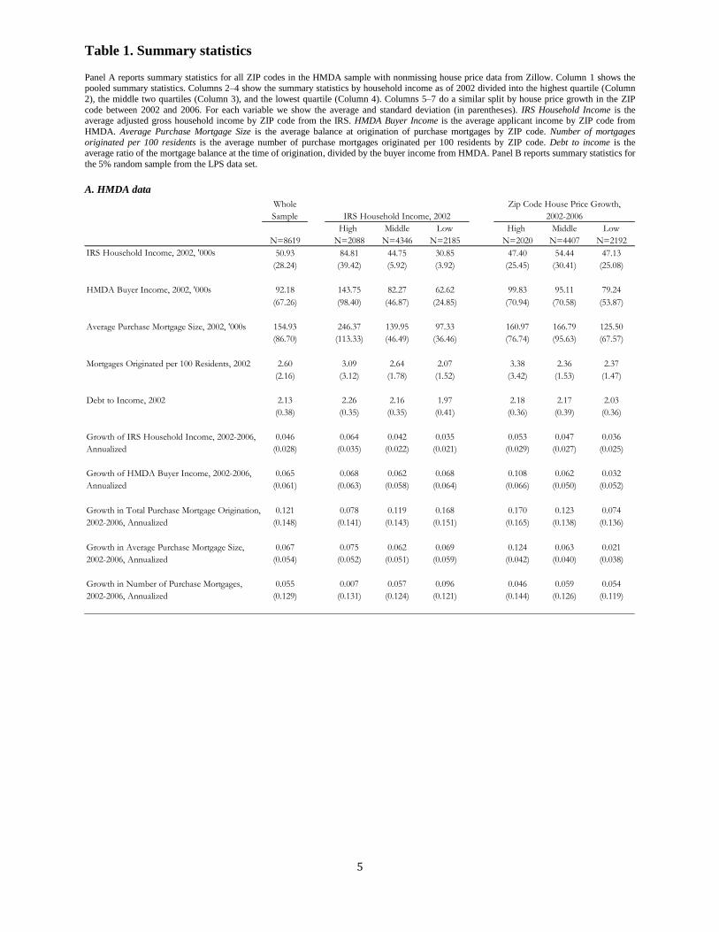
5

Table 1. Summary statistics Panel A reports summary statistics for all ZIP codes in the HMDA sample with nonmissing house price data from Zillow. Column 1 shows the pooled summary statistics. Columns 2–4 show the summary statistics by household income as of 2002 divided into the highest quartile (Column

2), the middle two quartiles (Column 3), and the lowest quartile (Column 4). Columns 5–7 do a similar split by house price growth in the ZIP

code between 2002 and 2006. For each variable we show the average and standard deviation (in parentheses). IRS Household Income is the average adjusted gross household income by ZIP code from the IRS. HMDA Buyer Income is the average applicant income by ZIP code from

HMDA. Average Purchase Mortgage Size is the average balance at origination of purchase mortgages by ZIP code. Number of mortgages

originated per 100 residents is the average number of purchase mortgages originated per 100 residents by ZIP code. Debt to income is the average ratio of the mortgage balance at the time of origination, divided by the buyer income from HMDA. Panel B reports summary statistics for

the 5% random sample from the LPS data set.

A. HMDA data

Whole

Sample

High Middle Low High Middle Low

N=8619 N=2088 N=4346 N=2185 N=2020 N=4407 N=2192

50.93 84.81 44.75 30.85 47.40 54.44 47.13

(28.24) (39.42) (5.92) (3.92) (25.45) (30.41) (25.08)

92.18 143.75 82.27 62.62 99.83 95.11 79.24

(67.26) (98.40) (46.87) (24.85) (70.94) (70.58) (53.87)

154.93 246.37 139.95 97.33 160.97 166.79 125.50

(86.70) (113.33) (46.49) (36.46) (76.74) (95.63) (67.57)

2.60 3.09 2.64 2.07 3.38 2.36 2.37

(2.16) (3.12) (1.78) (1.52) (3.42) (1.53) (1.47)

2.13 2.26 2.16 1.97 2.18 2.17 2.03

(0.38) (0.35) (0.35) (0.41) (0.36) (0.39) (0.36)

0.046 0.064 0.042 0.035 0.053 0.047 0.036

(0.028) (0.035) (0.022) (0.021) (0.029) (0.027) (0.025)

0.065 0.068 0.062 0.068 0.108 0.062 0.032

(0.061) (0.063) (0.058) (0.064) (0.066) (0.050) (0.052)

0.121 0.078 0.119 0.168 0.170 0.123 0.074

(0.148) (0.141) (0.143) (0.151) (0.165) (0.138) (0.136)

0.067 0.075 0.062 0.069 0.124 0.063 0.021

(0.054) (0.052) (0.051) (0.059) (0.042) (0.040) (0.038)

0.055 0.007 0.057 0.096 0.046 0.059 0.054

(0.129) (0.131) (0.124) (0.121) (0.144) (0.126) (0.119)

IRS Household Income, 2002

Zip Code House Price Growth,

2002-2006

IRS Household Income, 2002, '000s

HMDA Buyer Income, 2002, '000s

Average Purchase Mortgage Size, 2002, '000s

Mortgages Originated per 100 Residents, 2002

Debt to Income, 2002

Growth in Total Purchase Mortgage Origination,

2002-2006, Annualized

Growth in Average Purchase Mortgage Size,

2002-2006, Annualized

Growth in Number of Purchase Mortgages,

2002-2006, Annualized

Growth of HMDA Buyer Income, 2002-2006,

Annualized

Growth of IRS Household Income, 2002-2006,

Annualized

6

B. LPS data, 2002–2006 purchase mortgage cohorts (N = 272,077 for all cohorts)

Whole

Sample High Middle Low High Middle Low

Balance at Origination, 2003 cohort 188.69 276.80 167.36 118.35 197.94 204.49 148.47

N = 51,947 (140.31) (196.66) (93.23) (66.94) (151.53) (148.17) (97.60)

Credit Score (FICO), 2003 cohort 711.8 729.0 710.1 691.7 711.1 716.0 704.7

N = 44,750 (62.7) (53.8) (62.8) (67.5) (61.5) (61.1) (66.2)

3-Yr Delinquency Rate, 2003 cohort 0.037 0.015 0.038 0.070 0.027 0.033 0.057

3-Yr Delinquency Rate, 2006 cohort 0.183 0.115 0.177 0.271 0.301 0.131 0.148

IRS Household Income, 2002

Zip Code House Price Growth,

2002-2006

7

Table 2. Purchase mortgage origination and income Panel A shows regressions of growth in total purchase mortgage origination, the average purchase mortgage size, and the number of purchase mortgages originated at the ZIP code level on the growth rate of household income (from the IRS). For each measure we report the pooled OLS

regression, a regression with county fixed effects, and the between-county estimator. Growth rates are annualized and computed between 2002

and 2006. Panel B reports standard deviations for the IRS income and mortgage growth measures. Panel C shows fixed effects regressions of the logarithm of total purchase mortgage credit at the ZIP code level, the logarithm of average purchase mortgage size, and the logarithm of the total

number of purchase mortgages on the logarithm of household income. IRS data are available for 2002, 2004, 2005, and 2006 (2003 is excluded

from the panel regression). The sample includes ZIP codes with house price data from Zillow. Standard errors are clustered by county (shown in parentheses). *, **, and *** indicate statistical significance at the 10%, 5%, and 1% level, respectively.

A. Regressions of mortgage growth measures, 2002–2006

B. Standard deviation, income and mortgage growth, 2002–2006

C. Panel specification

Estimator: OLS Within Between OLS Within Between OLS Within Between

Growth IRS Household Income 0.368*** -0.182** 1.800*** 0.587*** 0.239*** 0.994*** -0.218** -0.402*** 0.672***

(0.109) (0.090) (0.275) (0.038) (0.026) (0.100) (0.091) (0.075) (0.232)

County FE - Y - - Y - - Y -

Number of observations 8,619 8,619 8,619 8,619 8,619 8,619 8,619 8,619 8,619

R2 0.00 0.33 0.07 0.09 0.68 0.15 0.00 0.31 0.01

Total Purchase Mortgage Average Mortgage Size Number of Mortgages

Between Within

Annualized growth, 2002-2006, N = 8619 Mean St. Dev. county SD county SD

IRS Household Income 0.046 0.028 0.018 0.024

Total Purchase Mortgage Origination 0.121 0.148 0.120 0.121

Average Purchase Mortgage Size 0.067 0.054 0.044 0.031

Number of Purchase Mortgages 0.055 0.129 0.102 0.107

Ln(IRS Household Income) 0.378*** 1.104*** 0.442*** 0.451*** -0.068 0.654***

(0.080) (0.095) (0.033) (0.048) (0.073) (0.075)

Ln(IRS Household Income) -0.137*** 0.010 -0.152***

x Year 2004 (0.021) (0.010) (0.018)

Ln(IRS Household Income) -0.246*** 0.020 -0.270***

x Year 2005 (0.026) (0.014) (0.021)

Ln(IRS Household Income) -0.382*** -0.015 -0.369***

x Year 2006 (0.027) (0.015) (0.023)

Zip Code FE Y Y Y Y Y Y

Year FE Y Y Y Y Y Y

Number of observations 36,299 36,299 36,299 36,299 36,299 36,299

R2 0.97 0.97 0.97 0.97 0.97 0.97

Total Purchase Mortgage

Origination Average Mortgage Size Number of Mortgages

8

Table 3. Origination and income at the transaction level

The table shows regressions of the logarithm of purchase mortgage size at the individual level on the logarithm of average household income in

the census tract (inferred using ZIP code household income from the IRS). The unit of observation is an individual loan in HMDA in ZIP codes

with nonmissing Zillow house price data. IRS data are available for 2002, 2004, 2005, and 2006. In Columns 2 and 4 the income variable is

interacted indicator variables for each year in the sample. Standard errors are clustered by county (shown in parentheses). *, **, and *** indicate

statistical significance at the 10%, 5%, and 1% level, respectively.

(1) (2) (3) (4)

Ln(IRS Household Income) 0.600*** 0.594*** 0.397*** 0.346***

(0.014) (0.018) (0.029) (0.039)

Ln(IRS Household Income) 0.038*** 0.075***

x Year 2004 (0.014) (0.012)

Ln(IRS Household Income) 0.026 0.079***

x Year 2005 (0.019) (0.016)

Ln(IRS Household Income) -0.041** 0.016

x Year 2006 (0.017) (0.016)

Year FE and county FE Y Y N N

Year FE and census tract FE N N Y Y

Number of observations 17,220,064 17,220,064 17,220,064 17,220,064

R2 0.23 0.23 0.29 0.29

9

Table 4. Purchase mortgage origination and income by income level as of 2002

The table shows OLS regressions of growth in total purchase mortgage credit, the average purchase mortgage size, and the number of purchase mortgages originated at the ZIP code level on the growth rate of household income (from the IRS). Growth rates are annualized and computed

between 2002 and 2006. ZIP codes are separated into quartiles based on the household income as of 2002. The “High” column includes the top

quartile, “Medium” includes the second and third quartiles, and “Low” includes the lowest quartile. In panel A we partial out county fixed effects estimated over the whole sample. Standard errors are clustered by county (shown in parentheses). *, **, and *** indicate statistical significance at

the 10%, 5%, and 1% level, respectively.

A. Within estimator

B. OLS, no county fixed effects

High Medium Low High Medium Low High Medium Low

Growth of IRS Household Income -0.191 0.218* 0.144 0.227*** 0.258*** 0.222*** -0.406*** -0.037 -0.125

(0.126) (0.118) (0.226) (0.034) (0.033) (0.061) (0.110) (0.107) (0.193)

County FE Y Y Y Y Y Y Y Y Y

Number of observations 2,088 4,346 2,185 2,088 4,346 2,185 2,088 4,346 2,185

R2 0.00 0.00 0.00 0.04 0.03 0.01 0.01 0.00 0.00

Total Purchase Mortgage Average Mortgage Size Number of Mortgages

High Medium Low High Medium Low High Medium Low

Growth of IRS Household Income 0.222* 1.398*** 1.734*** 0.432*** 0.766*** 0.869*** -0.197* 0.589*** 0.666***

(0.131) (0.139) (0.210) (0.056) (0.065) (0.086) (0.119) (0.117) (0.157)

County FE N N N N N N N N N

Number of observations 2,088 4,346 2,185 2,088 4,346 2,185 2,088 4,346 2,185

R2 0.00 0.05 0.06 0.08 0.11 0.10 0.00 0.01 0.01

Total Purchase Mortgage Average Mortgage Size Number of Mortgages

10

Table 5. Mortgage origination and growth in buyer income Panel A shows OLS regressions of growth in total mortgage credit, the average mortgage size, and the number of mortgages originated at the ZIP code level on the growth rate of average buyer income in the ZIP code (obtained from HMDA). Panel B shows OLS regressions of annualized

growth in total mortgage credit at the ZIP code level on the annualized growth rate of average buyer income in the ZIP code (from HMDA).

Results are split by the proportion of loans sold to Fannie Mae and Freddie Mac (the GSEs) as of 2006 and by the proportion of loans originated by subprime lenders as of 2006 (subprime lenders are defined by the HUD subprime lender list). Panel C shows the same regressions as in panel

A for total mortgage origination and the average mortgage size for alternative time periods. Growth rates are all annualized and computed

between 2002 and 2006. The sample includes ZIP codes with house price data from Zillow. Standard errors are clustered by county (shown in parentheses). *, **, and *** indicate statistical significance at the 10%, 5%, and 1% level, respectively.

A. Regression of mortgage growth measures, 2002–2006

B. Heterogeneity by propensity for income misreporting

C. Alternative time periods

Estimator: OLS Within Between OLS Within Between OLS Within Between

Growth of Buyer Income (HMDA) 0.524*** 0.369*** 0.828*** 0.539*** 0.282*** 0.725*** 0.002 0.117*** 0.079

(0.047) (0.047) (0.089) (0.033) (0.015) (0.025) (0.052) (0.040) (0.079)

County FE - Y - - Y - - Y -

Number of observations 8,619 8,619 8,619 8,619 8,619 8,619 8,619 8,619 8,619

R2 0.05 0.35 0.09 0.37 0.72 0.49 0.00 0.31 0.00

Total Purchase Mortgage Average Mortgage Size Number of Mortgages

High GSE

Fraction

Med GSE

Fraction

Low GSE

Fraction

High Subprime

Fraction

Med Subprime

Fraction

Low Subprime

Fraction

Growth of Buyer Income (HMDA) 0.335*** 0.387*** 0.348*** 0.470*** 0.313*** 0.375***

(0.077) (0.054) (0.098) (0.090) (0.059) (0.080)

County FE Y Y Y Y Y Y

Number of observations 2,203 4,355 2,062 2,120 4,326 2,174

R2 0.01 0.02 0.02 0.03 0.01 0.02

Growth in Total Purchase Mortgage Origination

1996-1998 1998-2002 2002-2006 2007-2011 1996-1998 1998-2002 2002-2006 2007-2011

Growth of Buyer Income (HMDA) 0.260*** 0.258*** 0.368*** 0.341*** 0.261*** 0.179*** 0.282*** 0.307***

(0.033) (0.024) (0.047) (0.029) (0.015) (0.015) (0.015) (0.015)

County FE Y Y Y Y Y Y Y Y

Number of observations 8,597 8,609 8,620 8,550 8,597 8,609 8,620 8,550

R2 0.57 0.44 0.35 0.48 0.46 0.57 0.72 0.64

Growth in Average Mortgage SizeGrowth in Total Purchase Mortgage Origination

11

Table 6. Mortgage refinancing and income Panel A shows regressions of growth in total refinancing mortgage origination, the average refinancing mortgage size, and the number of refinancing mortgages originated at the ZIP code level on the growth rate of household income (from the IRS). For each measure we report the

pooled OLS regression, a regression with county fixed effects, and the between county estimator. Growth rates are annualized and computed

between 2002 and 2006. Panel B shows fixed effects regressions of the logarithm of total refinancing mortgage credit at the ZIP code level, the logarithm of average refinancing mortgage size, and the logarithm of the total number of refinancing mortgages on the logarithm of household

income. IRS data are available for 2002, 2004, 2005, and 2006. The sample includes ZIP codes with house price data from Zillow. Standard

errors are clustered by county (shown in parentheses). *, **, and *** indicate statistical significance at the 10%, 5%, and 1% level, respectively.

A. Mortgage growth measures, 2002–2006

B. Panel specification

Estimator: OLS Within Between OLS Within Between OLS Within Between

Growth IRS Household Income -0.332** -1.200*** 1.684*** 0.459*** -0.005 1.064*** -0.651*** -1.100*** 0.696***

(0.149) (0.129) (0.231) (0.041) (0.030) (0.081) (0.115) (0.096) (0.178)

County FE - Y - - Y - - Y -

Number of observations 8,622 8,622 8,622 8,622 8,622 8,622 8,622 8,622 8,622

R2 0.00 0.55 0.05 0.05 0.75 0.16 0.02 0.48 0.02

Total Refinancing Origination Average Refi Mortgage Size Number of Refi Mortgages

Ln(IRS Household Income) -0.123 1.300*** 0.322*** 0.314*** -0.440*** 1.001***

(0.129) (0.129) (0.031) (0.050) (0.115) (0.098)

Ln(IRS Household Income) -0.502*** -0.001 -0.506***

x Year 2004 (0.026) (0.013) (0.020)

Ln(IRS Household Income) -0.604*** 0.015 -0.623***

x Year 2005 (0.039) (0.018) (0.027)

Ln(IRS Household Income) -0.717*** -0.002 -0.719***

x Year 2006 (0.044) (0.019) (0.031)

Zip Code FE Y Y Y Y Y Y

Year FE Y Y Y Y Y Y

Number of observations 36,265 36,265 36,265 36,265 36,265 36,265

R2 0.96 0.97 0.96 0.96 0.96 0.97

Total Refinancing Mortgage

Origination Average Mortgage Size Number of Mortgages