loan officer incentives, internal rating models and … loan officer incentives, internal rating...

1

Loan Officer Incentives, Internal Rating Models and Default rates

Tobias Berg,† Manju Puri,

‡ and Jörg Rocholl

§

May 2016

Abstract

There is increasing reliance on quantitative complex models, such as internal ratings based (IRB)

models for bank regulation, with much resources being spent on model validation exercises. We

argue that a significant cost of IRB models that is not well understood or monitored is the change

in loan officer incentives down the line. Using proprietary data on almost a quarter million loan

applications, we show loan officer incentives significantly skew ratings even if the quantitative

model is correct and there is no subjectivity in the system. These incentive effects have a first

order effect on bank profitability. Incentives influence the hard information reported by loan

officers and thus change the link between hard information and default probabilities in a way not

captured by regular model validation exercises. Banks and regulators need to take these effects

into account when using internal ratings for risk assessment and regulation.

We thank Sumit Agarwal, Matthew Bothner, Alejandro Drexler, Andre Güttler, Rainer Haselmann,

Andrew Hertzberg, Nadya Jahn, Adam Kolasinski, Alexander Libman, Jeff Ngene, Lars Norden, Felix

Noth, Nick Souleles, Sascha Steffen, Andrew Winton, the participants of the AFA meetings, San Diego,

NBER Corporate Finance meetings, FIRS conference, Minneapolis, Annual Conference on Bank

Structure and Competition, Chicago, Banking Workshop, Münster, Carefin-Bocconi conference, Milan,

CAFRAL conference, Mumbai, DGF meeting, Hannover, EFA meetings, Copenhagen, FMA meetings,

Atlanta, ISB conference, Hyderabad, Winter Workshop, Oberjoch, as well as participants of research

seminars at Bank of Canada, Bonn University, Cheung Kong Graduate School of Business, Beijing, Duke

University, ESMT, Frankfurt School of Finance and Management, Humboldt University Berlin, MIT,

New York Fed, New York University, Purdue University, Shanghai Advanced Institute of Finance,

University of British Columbia, University of Cologne, University of Southern California, University of

Toronto, U T Austin, and the World Bank. Berg acknowledges support from the Deutsche

Forschungsgemeinschaft (DFG).

† Bonn University, Email: [email protected]. Tel: +49 228 73 6103. ‡ Duke University and NBER. Email: [email protected]. Tel: (919) 660-7657.

§ ESMT European School of Management and Technology. Email: [email protected]. Tel: +49 30 21231-

1010.

2

1. Introduction

There has been much debate on the right way to regulate banks. The financial crisis of 2008

brought matters to a fore with many arguing that banks should be regulated in a way that

accurately measures the risk that they undertake. One of the consequences of changes in

regulations has been an increased reliance on sophisticated, complex, model-based regulation.

Internal rating based (IRB) models are at the heart of model-based regulation. IRB models are

used for a variety of critical bank and regulatory decisions including the use of risk weights in

Basel regulation (both Basel II and Basel III), stress testing purposes, statistical models for

securitization, and in loan granting and pricing decisions. Yet the consequences of IRB based

models and the effectiveness with which they are evaluated has been little studied.

Glaeser and Shleifer (2001) argue that the choice of sophisticated models needs to be

assessed by their costs of enforcement. We argue a significant additional cost of enforcement that

regulators have overlooked in model validation exercises is the change in incentives of loan

officers down the line in making loans, the effects of which can be economically large.

In this paper, we show that even when the quantitative model is correct with no

subjectivity in the system, the incentives of these loan officers can result in significantly skewing

of internal ratings. Using unique proprietary data on over a quarter million consumer loan

applications, we document this in a variety of ways. We further show that the economic effects of

underlying incentives and resulting skew of internal ratings are large.

The experiment setting that we employ is a unique data set from a major European bank.

An important feature here that makes our data particularly suitable for the question on hand is

that the quantitative model for making loans relies solely on hard information, while loan officers

3

are incentivized by loan volume. Common wisdom suggests that basing loans on hard

information should make the loan granting process more objective and thus less susceptible to

adverse incentives, e.g., cronyism and other dark aspects of discretion. Hence this setting is well

suited to the question of whether internal ratings based on quantifiable models are materially

skewed by loan officer incentives.

In particular, we address the following research questions. Do loan officers influence

internal ratings when ratings are based off quantifiable models? If so, is this economically

important? What are the implications for default rates and, ultimately, bank profitability such as

return on assets (RoA) or return on equity (RoE)?

In the setup we study, the loan officer acquires and feeds in hard information about the

customer (e.g., income, assets, etc.). The computer runs the underlying credit scoring model and

gives an accept/reject decision based on whether the loan is above the cut-off or not. If the

decision comes up as reject, the loan officer cannot override the decision or add soft information.

However, the loan officer can alter or update the information and do another scoring trial which

will bring up a new decision. Unknown to the loan officer, we are able to see how many times the

loan officer does a scoring trial and also what kind of information is added to each scoring trial.

In particular, we are able to see whether the number of scoring trials for loans that are near the

cut-off are different from other loans. We conduct two kinds of analysis to establish the link

between loan officer incentives and internal ratings. First, we take advantage of a change in the

cut-off and run a difference-in-difference analysis to establish the link between loan officer

incentives and internal ratings. Second, we run a regression discontinuity analysis in both regimes

with different cut-offs to see if loan officer behavior changes at the cut-off.

4

The cut-off rule induces an exogenous variation in “incentives to manipulate”: while loan

officers cannot earn an origination bonus for applications just below the approval threshold, they

can earn an origination bonus for loan applications just above the approval threshold. This set-up

therefore provides us with within-loan-officer variation in incentives, and also enables us to use

loan officer fixed effects in all our regressions.

We find there are more scoring trials for loan applications that do not pass in the initial

trial. The number of scoring trials increases as one gets closer to the cut-off boundary, and jumps

at the cut-off boundary. Interestingly, when the cut-off is changed, the jump in scoring trials

moves to the new cut-off point. These multiple scoring trials result in skewed (i.e. too optimistic)

ratings. Thus, the bank will overestimate the applicant's creditworthiness when granting these

loans. We further rule out alternative explanations and provide evidence that multiple scoring

trials are not due to the incorporation of soft information nor to an input of additional hard-to-

collect hard information, but rather than increased number of scoring trials actually lead to higher

default rates.

Finally, we analyze the economic importance of loan officer manipulations. We find that

while loans with multiple scoring trials have higher default rates, they do not carry higher interest

rates. For applications before January 2009, loans with multiple scoring trials in the rating

category directly above the cut-off have a 5 percentage point higher default rate and a 2

percentage point lower internal rate of return (IRR) than other loans with the same final rating.

Economic effects are somewhat smaller, but still highly economically significant after January

2009. The economic effects on bank profitability for the overall portfolio of consumer loans

across all rating categories are highly significant: multiple scoring trials lead to a decrease in the

internal rate of return (IRR) of 0.10 percentage points and a decrease in the return on equity

5

(RoE) of 1.50 percentage points. These numbers are clearly significant in economic terms. The

IRR after refinancing costs of the bank’s consumer loan portfolio is 0.9% and the RoE is 15%.

Thus, the reduction constitutes approximately 10% of the respective baseline values. The

profitability of the entire bank is lower, comparable to the average profitability of the German

banking sector (RoA of 0.4%, RoE of 8.4%).1 Thus, the reduction in the internal rate of return

and RoE amount to up to 25% of the bank and industry wide averages. Our results thus suggest

that bank profitability is adversely affected by the use of multiple scoring trials, with RoA and

RoE declining by 10-25% of their baseline values.

Our results suggest that loan officers' incentives can cause strategic manipulation of

information and thus significantly skew internal ratings even if internal ratings are determined

solely on hard information. Further, our results suggest that the quality of hard information is

highly contextual, so even hard information can be manipulated at the margin. These results have

clear implications for model validation tests: It is not sufficient for banks and regulators to look at

whether the underlying model is correct, even if there is no subjectivity in the system. Rather,

they need to look at agency problems and incentives of employees down the line as they can have

a first-order effect on the validity of model outputs.

Our paper relates to different strands of the literature. First, we complement Rajan, et. al.

(2015) and Behn, et. al. (2014). Rajan, et. al. (2015) show that bank incentives induced by the

originate-to-distribute model change the link between FICO score and default rates; while Behn

et. al. (2014) provide evidence suggesting bank-induced miscalibration of internal ratings to

reduce capital requirements. In contrast, in our paper, the bank does not use internal ratings for

1 The exact bank values for RoA and RoE are not disclosed as this could allow uncovering the identity of the bank.

For industry-wide averages for RoA and RoE see http://fsi.imf.org/fsitables.aspx.

6

regulatory purposes during our sample period. Hence our results do not come from the bank

deliberately inflating ratings to reduce capital requirements under the Basel II/III regulation.

Internal ratings can be influenced by incentives of top management. Alternatively, line officers

may skew internal ratings because of their own incentives. Our experiment allows us to focus on

the latter. We provide evidence that incentives of employees down the line matter for the

accuracy of internal ratings – even in a system that solely relies on objective hard information.

This suggests that regulators need to go beyond just evaluating the quantitative model in

assessing internal ratings and look carefully at the incentive effects down the line in

implementing the model.

Second, we contribute to the literature on agency problems within banks. Udell (1989)

and Berg (2015) provide evidence that the purpose of the loan review function in a bank is to

reduce agency problems between the bank and its loan officers. Hertzberg, Liberti, and Paravisini

(2010) show that a rotation policy affects loan officers' reporting behavior. Agarwal and Ben-

David (2015) analyze incentive schemes within a bank. Cole, Kanz and Klapper (2015) use a

laboratory experiment with loan officers in India to analyze the effects of different incentive

schemes on loan officer effort. We show that – in the presence of internal agency problems – loan

officers manipulate hard information whenever truthful reporting is incompatible with their

personal incentives.

Third, our paper relates to the literature that identifies hard information as a potential

solution for internal agency problems. Stein (2002) argues that the potential for agency conflict

between the bank and its loan officers is a function of how much soft information the agent has or

can produce hence this could lead to large, centralized banks relying on hard information to

7

reduce loan officer agency problems.2 Consistently, Berger et. al. (2005) find that large banks are

less willing to engage in informationally difficult loans for which soft information is more

important. Similarly, Liberti and Mian (2009) and Agarwal and Hauswald (2010) find borrower

proximity is related to the use of soft information. Our evidence suggests that even ratings based

on hard information can be manipulated depending on loan officer incentives. Thus the value of

hard information is highly contextual.

The rest of the paper is organized as follows. Section 2 describes our dataset and provides

descriptive statistics. Section 3 explains our empirical strategy. Section 4 presents the empirical

results. Section 5 concludes.

2. Data and descriptive statistics

A. Data and loan process

We obtain data on consumer loan applications and subsequent default rates from a major

European bank. These data comprise detailed information on 242,011 loan applications at more

than 1,000 branches of the bank between May 2008 and June 2010. From these 242,011 loan

applications, 116,969 materialize and data on the performance and defaults of these 116,969

loans are available until May 2011. Loans are granted to both existing and new customers.

During the loan application process, each customer is assigned an internal rating. The internal

rating ranges from 0.5 (best rating) to 24.5 (worst rating) which is mapped into 24 discrete rating

2 Paravisini and Schoar (2015) present a countervailing view where summaries of complex hard information can

enhance loan officer monitoring. Our paper also complements the findings of Garmaise (2015) who documents

borrower misreporting of collateral values.

8

classes ranging from 1 (best rating class) to 24 (worst rating class) which is solely based on hard

information.3 The inputs consist of five parts: First, an external score, which is similar to a FICO

score; second, a socio-demographic score, which is based on parameters such as age and sex;

third, an account score if the customer has a savings account with the bank; fourth, a loan score if

the customer already has a loan relationship with the bank; fifth a financial score which

aggregates income data, expenses, assets, and liabilities. Finally, these five parts are aggregated

into an overall internal rating. Under the Basel II/III regulation, inflated ratings can reduce capital

requirements. Thus, the bank itself can have incentives to inflate rating under Basel II/III.

However, during the period under study, the bank does not use these internal ratings for

regulatory purposes. Thus, our results are not contaminated by bank's incentives.

The loan application proceeds in the following way: First, the loan officer enters all the

necessary data into the system. If the loan is given, the written documentation, such as a copy of

the identification card and a salary certificate, has to be archived together with the loan

agreement. The bank's risk management function periodically checks the validity of this

documentation based on a random sample selection. If loan officers manipulate customer data,

they thus face a risk of being caught later on. However, no loan-by-loan checks are conducted

when the loans are granted.

Second, the loan officer requests a score from the internal rating system. This score

determines whether a loan shall be given and the interest rate charged for this loan. Loan

applications with an internal rating worse than the cut-off rating are automatically rejected by the

system and receive the status 'automatically rejected'. Loan applications with an internal rating

3 The rating is available as a continuous variable and we make use of the continuous version of the rating in the

regression discontinuity design.

9

better or equal to the cut-off rating receive the status 'open', and the risk-based pricing scheme

applies. The cut-off criterion is equal to a rating of 14.5 (mapped into rating class 14) until 31

December 2008. This means that all loan applications with a rating class of 14 or better can be

accepted. This cut-off criterion is changed to 11.5 (mapped into rating class 11) on 1 January

2009. To put these ratings into perspective, a rating class of 14 is comparable to a B rating based

on the Standard & Poor's rating scale; a rating class of 11 is comparable to a BB rating. The cut-

off criterion is changed as a result of growing concern about the status of the European economy

in the wake of the financial crisis. The management of the bank decides to follow a prudent

strategy and tighten lending standards in order to preserve the risk profile of the loan portfolio.

Third, the loan officer decides on how to proceed. She can either proceed with the

application as entered into the system if the status is not 'automatically rejected', abort the loan

application, or change any of the input parameters and request a new internal rating, i.e. initiate a

new scoring trial. There are 442,255 unique scoring trials for the 242,011 loan applications ─ an

average of 1.83 scoring trials per loan application. Only the results of the last scoring trial are

recorded in the official systems of the bank, while all former trials are deleted. The only

exception is one specific risk management system used in this paper that archives each scoring

trial separately. Loan officers do not know that all scoring trials are recorded in this system, and

the bank's risk management function has not used this information so far.

There are five major advantages of our setup: First, each separate scoring trial is recorded

in the database. Second, loan officers are subject to a random review process. Therefore, they

have an incentive to report truthfully as long as truthful reporting is not incompatible with their

personal incentives. Third, we have information on individual loan officers which gives us the

possibility to analyze incentives across individual loan officers. Fourth, the cut-off rating was

10

changed during our sample period without any other change in the rating or incentive system.

This gives us the unique opportunity to analyze the effect of tighter lending standards on loan

officers' behavior. Fifth and finally, our dataset contains default information which enables us to

link loan officer incentives and lending standards to actual defaults.

B. Loan officer incentives

Loan officers receive a fixed salary and a bonus. The bonus is based on performance and can

make up to 25 percent of the fixed salary. The bonus period coincides with the calendar year, i.e.,

loan officers are evaluated based on their performance from January to December of each

calendar year. The bonus depends on the volume of the loans that a loan officer generates in a

given year and the conditions at which these loans are granted, but not on the default rates of

these loans. In particular, loan officers receive a fee for each successful loan application. The fee

is based on the expected net present value (NPV) for the bank. Interest rates are largely

determined by rating, with better ratings receiving lower interest rates. The resulting fee is

usually higher for higher-rated loans. Thus, a loan officer benefits from a better rating for a loan

applicant for two reasons: First, a higher rating increases the likelihood of a loan application

being successful. Second, a better rating results in a higher fee for a successful loan application.

The average fee for a successful loan application is approximately 20 times larger than the fee

increase for a one-notch higher rating class. Thus, the first-order incentive effect comes from

ensuring that the rating meets the minimum-creditworthiness condition, while further rating

improvements have a second-order effect. At the same time, there is a significant pressure to

perform well. Each week, or even during each week, 'run lists' are compiled to rank each

individual loan officer. We collectively refer to both monetary and non-monetary incentives as

11

loan officer incentives and analyze how these incentives affect loan officer behavior in a hard

information environment.

The cut-off rule induces an exogenous variation in “incentives to manipulate”: while loan

officers cannot earn an origination bonus for applications just below the approval threshold, they

can earn an origination bonus for loan applications just above the approval threshold. This set-up

therefore provides us with within-loan-officer variation in incentives, and also enables us to use

loan officer fixed effects in all our regressions.

While lending standards are tightened in January 2009, the performance targets that are

given to individual loan officers remain unchanged. This means that loan officers are faced with

the same targets but a much smaller customer base that can make the cut-off rating after the

change. This provides an incentive to loan officers to manipulate customer information to achieve

their targets. So while loan officer compensation and bonus criteria do not vary over time, the

change of the cut-off provides different incentives to manipulate client data. It is this variation

that we aim to analyze in this paper.

After origination, the loan is transferred to an internal portfolio management unit, and the

loan officer is no longer responsible for the performance of the loan. The compensation of the

loan officer does therefore not depend on whether the loan defaults.

C. Descriptive statistics

Table 2 presents descriptive statistics on loan application level (Panel A), scoring trial

level (Panel B) and loan officer level (Panel C). All variables are explained in Table 1. The

information on the loan application level in Panel A is based on the last scoring trial per loan

application. This is the only information that is available in the systems of the bank, apart from

12

the single risk management system used for the analysis in this paper that tracks every trial. 13

percent of the loan applications have a rating below the cut-off and are therefore automatically

rejected. On average, loan officers use the scoring system 1.83 times per loan application. The

average acceptance rate is 48 percent, i.e. 48 percent of the loan applications are accepted by both

bank and customer. The average loan amount is EUR 13,700, the average number of borrowers

per loan application is 1.34, the average age of a borrower is 45.24 years, and his average net

income per month is EUR 2,665. If a loan application has several borrowers, e.g., husband and

wife, then parameters such as net income per month are aggregates over both borrowers with the

only exception being the age, where the average age is reported. 63 percent of the customers are

relationship customers who have either an existing account or another loan with the bank. The

information about the internal rating, which ranges from 0.5 (best) to 24.5 (worst), shows that the

average rating amounts to 8.40. Table 3 provides a mapping from internal rating classes to

probability of default estimates. This mapping comes from bank estimates and constitutes the

probability of default estimates the bank assigns to a given rating class. The risk model is

generally well-calibrated, with probabilities of default increasing roughly uniformly across rating

grades. For example, for an internal rating class of 12, the bank expected an annual default rate of

3.064%. For a one notch better rating (rating class 11) the probability of default estimate is

2.275%, i.e. 26% lower. A one notch improvement in the internal rating is associated on average

with a 20-30% lower probability of default estimate (see column (4) in Table 3). Given the

paucity of literature on this subject, a convincing example of a well-calibrated risk model is

arguably a contribution to the literature as well. The cut-off rating was set at 14.5 between May

2008 and December 2008 and at 11.5 between January 2009 and June 2010. 28 percent of our

observations come from the earlier period, while 72 percent come from the latter period. Panel B

13

of Table 2 shows that 20 percent of the scoring trials result in a rating below the cut-off. This is

significantly higher than the 13 percent from the last trial, as shown in Panel A, and indicates

rating inflation, i.e., internal ratings are on average moved upwards with further trials. There is an

unconditional likelihood of 45 percent of observing another subsequent scoring trial for the same

loan application. Panel C shows that the 242,011 loan applications in our sample are arranged by

5,634 loan officers. During our sample period, an average loan officer uses the scoring system

78.50 times for 42.96 different loan applications of which 20.78 loans materialize, i.e. are finally

accepted by both bank and customer.

Table 4 provides a concrete example on the workings of the different scoring trials. In this

example, on 4 May 2009, a loan officer enters an application for a consumer loan of EUR 4,000

and records, among other parameters, existing liabilities of the customer of EUR 23,000 and a

monthly net income of EUR 1,900. The resulting internal rating of 12 is worse than the cut-off

rating of 11, therefore the loan application is automatically rejected by the system. The loan

officer subsequently increases the income to EUR 1,950 and decreases the liabilities to EUR

10,000. These two changes result in a new rating of 11 so that the loan application can be

accepted. However, the loan officer then decides to manually reject the loan application and

corrects the liability amount to EUR 19,000. As this change results again in a rating below the

cut-off, the loan officer reverses the liabilities back to EUR 10,000 and books the loan into the

system. This loan application provides a particular striking example of a manipulation around the

cut-off as the final amount for the liabilities of EUR 10,000 is clearly not a correction of a

previously misspecified value. This is the type of behavior that we would like to analyze more

thoroughly in this paper.

14

3. Empirical strategy

A. Loan officer incentives and internal ratings

The cut-off rating substantially affects loan officer incentives, as only loan applications

with ratings better than or equal to the cut-off rating can generate fee income. The change of the

cut-off rating during our sample period provides us with a clear identification strategy. Our

treatment group is the set of loan applications with an initial rating class of 12-14, i.e. those loan

applications that – based on the initial rating – can be granted before January 2009 but have to be

rejected after January 2009. We select loan applications with an initial rating class of 9-11 as the

control group, these loan applications are sufficiently close to the cut-off and can be granted

throughout our total sample period. We then estimate the following regression for all loan

applications with an initial rating class between 9 and 14:

Log(NumberOfTrials) = β1 Treated + β2 PostJan2009 + β3 Treated x PostJan2009 + δ X + ε (1)

where NumberOfTrials is the number of scoring trials, Treated is a dummy variable equal

to 1 for loan applications with an initial rating class between 12-14 and 0 for loan applications

with an initial rating between 9-11, PostJan2009 is a dummy equal to 1 for loan applications

during or after January 2009, Treated x PostJan2009 is the interaction term between

PostJan2009 and Treated and X is a set of control variables taken from the first scoring trial

including loan, customer and loan officer characteristics as well as loan officer and time-fixed

effects. The coefficient of interest is β3: a positive β3 suggests that loan officers use a higher

number of scoring trials after January 2009 for rating classes 12-14, i.e. for those rating classes

that had to be rejected after January 2009. The identifying assumption is that the number of

15

scoring trials would have evolved in a parallel fashion over time for rating classes above (9-11)

and below (12-14) the cut-off absent a change in the cut-off. We discuss the parallel trend

assumption as well as the estimation method in more detail in the results section.

Multiple scoring trials for a single loan application reflect loan officer behavior: Instead

of aborting a loan application, a loan officer decides to give it another try using a revised set of

parameters. Multiple scoring trials affect internal ratings, probability of default estimates (PDs),

and – for the Basel II/III internal-rating based approach – regulatory risk weights (RW). To

analyze the effect of the cut-off on final internal ratings, probability of default estimates, and

regulatory risk weights, we repeat the analysis above using the change in the internal rating, the

probability of default, and the risk weights, respectively, from the initial to the final scoring trial

as the dependent variable:

RatingChange = β1 Treated + β2 PostJan2009 + β3 Treated x PostJan2009 + δ X + ε (2a)

PDChange = β1 Treated + β2 PostJan2009 + β3 Treated x PostJan2009 + δ X + ε (2b)

RWChange = β1 Treated + β2 PostJan2009 + β3 Treated x PostJan2009 + δ X + ε (2c)

where RatingChange is the difference between the internal rating from the final scoring

trial and the internal rating from the initial scoring trial, PDChange is the difference between the

logarithm of the PD-estimate from the final scoring trial and the logarithm of the PD-estimate

from the initial scoring trial, and RWChange is the difference between the logarithm of the Basel

IRB (internal rating based) risk weight from the final scoring trial and the logarithm of the Basel

IRB risk weight from the initial scoring trial. We expect the rating change as well as the change

in the probability of default estimate and risk weight to be negative (for example, from an initial

rating class of 12 to a final rating class of 11 with a corresponding lower probability of default

16

estimates and lower risk weight), in particular for the loan applications with a rating class of 12-

14 after January 2009. Again, we discuss the estimation method in more detail in the results

section.

An analysis which would have been natural in the absence of the change in the cut-off is

regression discontinuity. We therefore also estimate the following regression discontinuity

regression for each time period (before cut-off change, after cut-off change) separately:

Log(NumberOfTrials) = β1 CutOffDummy + f(DifferenceToCutOff)

+ CutOffDummy x g(DifferencToCutOff) + δ X + ε (3)

where the dependent variable is the logarithm of the number of scoring trials (from

regression (1)), DifferenceToCutOff is the re-centered running variable, i.e. the internal rating less

the cut-off rating, and the function f and g are higher-order polynomials of this re-centered

running variable. Effectively, the regression above fits higher-order polynomials on the left- and

right-hand side of the cut-off, with the coefficient β1 denoting the jump in the number of scoring

trials at the cut-off. 4

B. Economic impact

In the next step, we estimate the economic impact of loan officer behavior when loans are

granted based on hard information. In particular, we provide evidence how this behavior affects

default rates as well as interest rates, and, as a consequence, the profitability of these loans. This

4 We also estimate regression (3) using the dependent variables from (2a), (2b), and (2c) instead of the number of

scoring trials (i.e., change in the rating, probability of default estimate, and Basel IRB risk weight). The results are

very similar to those in the baseline specification and are available upon request.

17

section serves two main objectives: First, it is important to understand whether loan officer

misbehavior harms profitability in a meaningful way. Second, this analysis helps to distinguish

between the different hypotheses as to why loan officers use multiple scoring trials.

For the latter, changes in the internal rating due to multiple scoring trials can be due to

loan officers manipulating information they have about the customer in order to increase their

income (information manipulation hypothesis) or loan officers inputting wrong hard information

for customers where they have positive soft information (soft information hypothesis) or loan

officers honestly correcting a false entry from a former trial (closer examination hypothesis). If

the information manipulation hypothesis was true, we should see a positive systematic effect of

the number of scoring trials on default rates and profitability. If the other two hypotheses were

true, there should be no or even a negative effect. We therefore estimate the impact of multiple

scoring trials on default rates, interest rates, and the internal rate of return (IRR):

DefaultDummy = f(β1 log(NumberOfTrials), δ X, ε) (4a)

InterestRate = f(β1 log(NumberOfTrials), δ X, ε) (4b)

IRR = f(β1 log(NumberOfTrials), δ X, ε) (4c)

where DefaultDummy is a dummy variable equal to one if the loan defaults within the first

12 months after origination, InterestRate is the contractual interest rate of the loan, and IRR is the

internal rate of return. The internal rate of return is calculated as

IRR = interest rate – default rate dummy x loss given default – operating cost (5)

18

using a 40% loss given default assumption and a 3% operating cost assumption.5

The variable log(NumberOfTrials) is the logarithm of the number of scoring trials, X is a set of

control variables taken from the last scoring trial of the loan (i.e. the scoring trial that enters the

bank systems) including various fixed effects. The function f is a link function such as the logistic

function. Again, details on the estimation method are discussed in section 4.

4. Empirical results

A. Loan officer incentives and internal ratings

A1. Univariate results

We compare the average number of scoring trials before and after the change in the cut-

off rating. Figure 1 shows the results for the comparison of the accepted loans, while Figure 2

shows the respective results for all loan applications. In Figure 1, we conduct the comparison

based on the rating class in which a loan is finally accepted. The figure shows that the number of

scoring trials is quite similar before and after the change in the cut-off rating for rating classes 1

to 10. Also, as the cut-off rating class is decreased to 11 in January 2009, there are no more loans

in rating classes 12 to 14 after this change. The most striking result is the significant increase in

the number of scoring trials after January 2009 for the loans that are finally accepted in rating

class 11. This evidence suggests that loan officers try much harder, by using more scoring trials,

5 The 40% loss given default assumption is based on bank-internal data. The 3% operating cost assumption is a best

estimate including upfront costs and recurring costs. Please note that the 3% operating cost assumption only affects

the level of the IRR, but none of our regression results that rely on cross-sectional differences.

19

to move loans above the cut-off rating after the change. A similar pattern can be found in Figure

2. Here we conduct the comparison based on the initial rating that a loan application receives.

Here, loan applications with an initial rating class between 1 and 11 do not exhibit different

patterns before and after the change in the cut-off rating. In strict contrast, there are significantly

more scoring trials for loan applications with an initial rating class between 12 and 14 after the

change, i.e. for those loan applications that fall just below the cut-off rating, but which the loan

officer can potentially move above the cut-off rating with additional scoring trials. For the

remaining rating classes 15 to 24, the number of scoring trials decreases after the change. These

rating classes are now more remote from the cut-off rating so that the incentives for the loan

officer to use more scoring trials are reduced.

A2. Multivariate results

Difference-in-difference estimator

We now estimate a multivariate model [regression (1)] to control for other factors that

may drive our results. These control factors comprise loan, customer and loan officer

characteristics. In particular, we use a dummy to control for the effect of being a relationship

customer, the logarithm of the customer's age, the logarithm of his income, and rating fixed

effects to control for the creditworthiness of the customer. On the loan side, we control for the

size of the loan, which can be regarded as a proxy for the fee potential, and for the number of

borrowers. All these variables are taken from the initial scoring trial. On the loan officer level, we

control for the past average number of trials per loan application and the past absolute number of

trials. Both measures are averaged over the previous three months and transformed on a log-

20

scale. As a third control variable on the loan officer level, we use the prior 3-months success rate

of the loan officer, measured as the ratio of successful loan applications, i.e. loan applications that

are accepted by bank and customer, and total loan applications. All variables are explained in

Table 1. Finally, we add time fixed effects (monthly) as well as loan officer fixed effects. To

account for possible autocorrelation at the branch level, we cluster standard errors accordingly.

We use a linear model to estimate (1). Linear models are able to accommodate a large

number of fixed effects without giving rise to the incidental parameter problem (Neyman and

Scott (1948)). Given that the number of scoring trials is a count variable, an alternative is to use a

Poisson model or a negative binomial model.6

Table 5 tests the parallel trend assumption by examining the pre-trend as suggested in

Roberts and Whited (2012). Column (1) regresses the logarithm of the number of scoring trials

on a time trend, the treated dummy (equal to 1 for rating classes 12-14) and an interaction term

between the treated dummy and the time trend. Column (2) and (3) add customer, loan, and loan

officer characteristics as well as various fixed effects. Column (4) narrows the sample to one

quarter before the change in the cut-off and columns (5) and (6) narrow the treated and control

group to +/- 1 notch and +/- 0.5 notches around the new cut-off of 11.5. In all specifications, the

interaction term is economically and statistically insignificant – suggesting that there are no pre-

event differences in the trends of treatment and control group. There is a difference in levels

between treatment and control group, i.e. the treatment dummy is significant in column (1) and

(2). While differences in levels do not invalidate the difference-in-difference design, they can

make the difference-in-difference estimator sensitive to the functional form of the regression

6 Results for the Poisson and negative binomial model are very similar and are available on request.

21

function. However, the difference vanishes once we restrict the sample to +/- 1 notch around the

new cut-off of 11.5 in column (5).7

Table 6 shows the results for regression (1). We start in column (1) by regressing the

logarithm of the number of scoring trials on a time trend, the treated dummy (equal to 1 for rating

classes 12-14) and an interaction term between the treated dummy and the time trend. The change

in the cut-off in January 2009 affected the rating classes 12-14. It increased the number of scoring

trials by 21% for these ratings, which is significant at the 1 percent level. Columns (2) and (3)

add customer, loan and loan officer characteristics as well as rating, time and loan officer fixed

effects. The results for the interaction term remain economically and statistically highly

significant in all specifications. Column (4) narrows the sample to one quarter before and after

the change in the cut-off. This specification therefore helps to establish that the increase in the

number of scoring trials for rating classes 12-14 is concentrated around January 2009. Column

(5) and (6) further narrow the treatment and control group from +/- 3 notches around the new cut-

off of 11.5 to +/-1 notch (column (5)) and +/-0.5 notches (column (6)) – thus ensuring that

treatment and control group have internal ratings as similar as possible. The coefficient on the

interaction term increases from 20% (column (3)) to 41% (column (6)). Thus, the change in the

cut-off caused loan officers to use 20-41% more scoring trials for the affected rating classes (12-

14). These results are consistent with the descriptive evidence: Multiple scoring trials are in

particular used for ratings worse, but close to, the cut-off (Figure 2). The initial loan amount is

highly statistically and economically significant with a coefficient estimate between 0.130 and

0.155. An increase in the initial loan amount from the median loan amount of EUR 10,000 by one

7 This effect cannot be seen from Table 4 as we do not show rating fixed effects. In column (5) and (6), the

difference between the rating fixed effect for an internal rating of 11 and 12 are not significantly different.

22

standard deviation (EUR 10,665) to EUR 20,665 therefore leads to an increase in the number of

scoring trials by ln(20,665/10,000)·0.155=11.2 percent. The results here are consistent with the

notion that loan officers move the ratings in particular for larger loans, as they receive a fee that

is proportional to the loan amount.

What are the resulting effects of the change in the cut-off on internal ratings? So far, we

have used the number of scoring trials as the dependent variable to provide causal evidence that

loan officer behavior changes with the change in cut-off. Now we turn to the effects on the

internal rating, the probability of default estimate, and Basel IRB risk weights. We thus estimate

regression (2a)-(2c) with the change in the internal rating, probability of default estimate, and

Basel IRB risk weight, respectively, between the initial and the final scoring trials as the

dependent variable. A negative change implies that the internal rating from the final scoring trial

is better than the internal rating from the initial scoring trial, while the probability of default

estimate and the Basel IRB risk weight from the final scoring trial are lower than the

corresponding values from the initial scoring trial. Table 7 presents the results using the

specification from column (3) in Table 6, i.e., the specification using the total sample period and

all control variables and fixed effects. The change in the internal rating between initial and final

scoring trial caused by the change in the cut-off is negative and significant at the 1 percent level

(see column (1) in Table 7). The coefficient on the interaction term is – 0.265– suggesting that

the change in the cut-off caused loan officers to revise the internal rating upwards by

approximately a quarter notch on average for loan applications with an initial rating class of 12-

14. Column (2) of Table 7 shows the results for the change in the probability of default estimate

as the dependent variable and exhibits a coefficient on the interaction term of -0.086 (see column

(2) in Table 7). Thus, probability of default estimates decrease by approximately 9% due to loan

23

officer misbehavior for the rating classes 12-14. Column (3) in Table 7 provides estimates for the

change in the Basel IRB risk weights from the initial to the final scoring trial. Again, the effect is

negative and highly significant (-0.027, significant at the 1 percent level).

Regression discontinuity

In the analysis above we took advantage of an exogenous change in the cut-off rating to

identify the causal effect of loan officer incentives on the number of scoring trials using a

difference-in-difference estimator. An analysis that would have been natural in the absence of

such a change is regression discontinuity. The basic idea of regression discontinuity is to fit a

regression function on both the left-hand side and the right-hand side of the cut-off and compare

the predicted values of these two regression functions at the cut-off point (Thistlewaite and

Campbell (1960), Imbens and Lemieux (2008), Keys, Mukherjee, Seru, and Vig (2010), and

Roberts and Whited (2012)). If the predicted value at the cut-off using data from the right-hand

side differs significantly from the predicted value at the cut-off using data from the left-hand side,

this can be attributed to the different incentives prevalent on either side of the cut-off. The

regression discontinuity approach relies on a no-manipulation assumption of the running variable,

i.e. the initial rating. Economically, this is not an issue here, as the loan officers do not know that

individual scoring trials are recorded. Hence, there is no reason to manipulate the initial scoring

trial. Nonetheless, we conduct a formal statistical test developed by McCrary (2008) which tests

for a discontinuity in the density of the running variable at the cut-off point. Indeed, we do not

find any evidence for a discontinuity in the density of the initial internal rating at the cut-off point

(Panel I of Table 8). In striking contrast, we do find a highly significant discontinuity in the

density of the final internal rating at the cut-off point (Panel I of Table 8).

24

Formal techniques used in the literature either use a polynomial model or a local linear

regression. Furthermore, covariates can be used to control for possible discontinuities in any of

the explanatory variables. We use both of these models (polynomial and local linear regression)

with and without covariates both before and after the change in the cut-off rating. As the

dependent variable, we use the logarithm of the number of scoring trials. In all cases, we find a

significant jump in the number of scoring trials at the cut-off rating (Panel II of Table 8). The

estimate of the jump in the number of scoring trials at the cut-off rating ranges from 0.265 to

0.358 (see Panel II of Table 8) which is very close to the estimates of 0.209 to 0.410 from the

difference-in-difference estimator from Table 6.

Exploring the patterns of loan officer behaviour

The analysis above demonstrates that loan officers use multiple scoring trials to manipulate

ratings. In the following, we further explore the patterns of this behavior. In particular, we first

look at whether multiple scoring trials are only used by a few loan officers or whether this

behavior is widely spread among all loan officers. We then analyze predictable patterns of

misbehavior at the end of the incentive period, i.e., at the end of the calender year.

Figure 3 provides the density of the average number of scoring trials per loan officer. On

the one hand, there are very few loan officers who use only one or close to one scoring trials on

average. On the other hand, there are very few loan officers who use more than three scoring

25

trials on average. These figures suggest that the use of multiple scoring trials is widely spread

among (almost) all loan officers.8

Figure 4 depicts the end-of-year effect. Our main variable of interest is a manipulation-

dummy which is equal to one if the initial scoring trial is worse than the cut-off and the final

scoring trial is better than the cut-off, i.e., the loan application has been pushed by the loan officer

over the cut-off. We split the group of loan officers into "high success" and "low success" loan

officers, where the latter are those loan officers in a given month whose success rate is lower than

50%. The success rate is measured as accepted loans over the past 9 months divided by total loan

applications handled over the past 9 months. Figure 4 shows a clear wedge between high success

and low success loan officers towards the end of the year, with low success loan officers

manipulating more towards the end of the year.9 These results are consistent with low success

rate loan officers being below their targets, and thus using multiple scoring trials to achieve their

sales target in a given year.10

B. Economic impact

B1.1 Univariate results

We compare default rates, interest rates, and internal rates of return (IRR) for loans with

more than two scoring trials to those for loans with two or less scoring trials. The default rate of a

8 We have also reproduced Figure 3 on the branch level, showing that manipulation is widespread across branches as

well. Results are available upon request.

9 Multivariate results (available upon request) confirm the univariate evidence from Figure 4.

10 Please not that we do not have access to the sales targets for each individual loan officer. If these were available,

one could more directly test this conjecture by constructing a dummy variable "Actual < Target ".

26

loan is measured over a time horizon of 12 months after the origination of the loan and IRRs are

determined according to equation (5). The results are presented in Table 9 and are reported

separately for each rating class before and after January 2009.11

Panel A provides results for

default rates, Panel B for interest rates, and Panel C for IRRs.

If loan officers indeed manipulate information and use multiple scoring trials to generate

more loans, then the difference in default rates between loans with more than two trials and loans

with two or less trials should primarily exist just above the cut-off, where the loan officer can use

multiple scoring trials to move a loan from below to above the cut-off. The results show that the

difference in default rates is indeed statistically and economically significant at the cut-off rating

class of 14 before January 2009 and 11 after January 2009, respectively. For the rating class 14

before January 2009, the default rate is 7.09% for loans with one or two trials, while it is 12.15%

for loans with more than two trials. Similarly, for the rating class 11 after January 2009, the

default rate is 7.83% for loans with one or two trials, and it is 10.11% for loans with more than

two trials. We further explore these results using a difference-in-difference setting by comparing

the difference in default rates for the rating class just below the cut-off rating to the difference in

default rates for the rating class one and two notches above the cut-off rating. This estimate is

highly significant both before and after January 2009.12

For example, before January 2009, the

default rate for loans with a rating class of 14 with more than two scoring trials is 5.06% higher

than the default rate for loans with two and less trials (12.15% versus 7.09%). This difference is

11 Realized default rates are on average higher than the expected default rates tabulated in Table 3. This is not

surprising given the poor macroeconomic conditions during our sample period, in particular the large drop in GDP in

2009.

12 These results are available upon request.

27

only 0.486% for a rating of 12 and the difference-in-difference estimate of 4.57% is significant at

the 1% level. Similar, after January 2009, the difference between loans with more than two

scoring trials and loans with two and less scoring trials is 2.29% for a rating class of 11. It is -

0.17% for a rating of 9, with the difference-in-difference estimate of 2.45% again being

significant at the 1% level.13 These results provide further evidence that the use of several scoring

trials is driven by loan officers’ manipulation of information with the goal to generate more

loans.

Higher default rates are not per se harmful for the bank as long as they are compensated

for by higher interest rates. We thus analyze interest rates in Panel B of Table 9. Interest rates for

loans with more than two scoring trials are very similar to interest rates for loans with two or less

scoring trials. This also holds directly above the cut-off: Before January 2009, loans with two or

less scoring trials have an interest rate of 10.83%, while the average interest rate for loans with

more than two scoring trials is even slightly lower (10.79%). After January 2009, interest rates

for a rating class of 11 (i.e., directly above the cut-off) are slightly higher for loans with more

than two scoring trials (10.06%) than for loans with two or less scoring trials (10.02%). However,

the difference of 0.04% is by far not enough to compensate for the increase in default rates of

2.283% (see Panel A, column B3).

Panel C combines the evidence on default rates and interest rates and provides results for

internal rates of return (IRR). For the rating grades directly above the cut-off, IRRs are 2.06%

(before January 2009) and 0.87% (after January 2009) lower for loans with more than two

13 The detailed results for the difference-in-difference estimates are available upon request.

28

scoring trials than for loans with two or less scoring trials. Given average IRRs of 5%, these are

highly economically significant magnitudes.

B1.2 Multivariate results

In the multivariate tests, we control for customer, loan and loan officer characteristics,

and the control variables are thus identical to the ones used in Table 6. We estimate regression

(4a)-(4c) using a linear probability model to address the incidental parameter problem.14

Columns (A1)-(A3) in Table 10 provide multivariate results for Panel A of Table 10, i.e.,

it uses the default rate over the first 12 month after loan orgination as the dependent variable. We

report a step-by-step development of our regression without control variables in column (A1),

with customer, loan, and loan officer characteristics in column (A2) and with rating, time, and

loan officer fixed effects in column (A3). In all specifications, we report standard errors clustered

by branch. The results show that the number of scoring trials is positively associated with the

default rate. In the full specification, including rating fixed effects (based on the final rating), the

coefficient is 0.4%. The results are statistically significant throughout at the 1 percent level. The

effect is also economically highly significant. Increasing the number of scoring trials from the

14 Standard logistic models suffer from the incidental parameter problem (Neyman and Scott (1984)), i.e. the

structural parameters cannot be estimated consistently in large but narrow panels. There are two possible ways to

circumvent the incidental parameter problem: First, a conditional logistic regression can be estimated (Chamberlain

(1980), Wooldridge (2002)). This approach has the drawback that the estimator is no longer efficient (Andersen

(1970)) but it yields consistent estimates of the structural parameters. Second, we can use a linear probability model

which leads to both efficient and consistent estimates of the structural parameters. We follow Puri, Steffen, and

Rocholl (2011) and use the latter approach to estimate regression (4). Results for the conditional logit model are

available upon request.

29

median of 1 scoring trial by one standard deviation (1.63 scoring trials) to 2.63 scoring trial leads

to an increase in the default rate of approximately 0.3-0.4%.15

Compared to the unconditional

default rate of 2.49% this is a relative increase in the default probability of 12-16%. We also

observe that the experience of the loan officer (3-months absolute number of scoring trials)

positively predicts the default rate. This suggests that experienced loan officers are more efficient

at manipulating the internal rating in the desired direction and magnitude and therefore need

fewer trials to achieve the desired result. In results reported in Appendix Table 1, we further

provide evidence that higher default rates are in particular driven by very short scoring trials

(lasting less than a minute) and changes to costs and liabilities. These facts provide further

evidence that it is not additional information that is driving multiple scoring trials, providing

further support for the information manipulation hypothesis.

Column (4) in Table 10 reports results using the interest rate as the dependent variable.

The coefficient on Log(Number of trials) is economically small and statistically insignificant. We

conclude that loans with a high number of scoring trials do not have significantly larger interest

rates.

Column (5) in Table 10 combines the evidence from default rates and interest rates and

uses the internal rate of return as the dependent variable. This column thus provides the economic

impact of loan officer behavior after taking into account both changes in default rates and interest

rates from using multiple scoring trials. The effect of multiple scoring trials is negative and

significant. Increasing the number of scoring trials from the median of 1 scoring trial by one

standard deviation (1.63 scoring trials) to 2.63 scoring trials decreases the IRR by 0.16

15 Increasing the number of scoring trials from 1.00 to 2.63 increases the log by ln(2.63)=0.97. Multiplying the

coefficient of 0.3-0.4% by 0.97 yields the stated result.

30

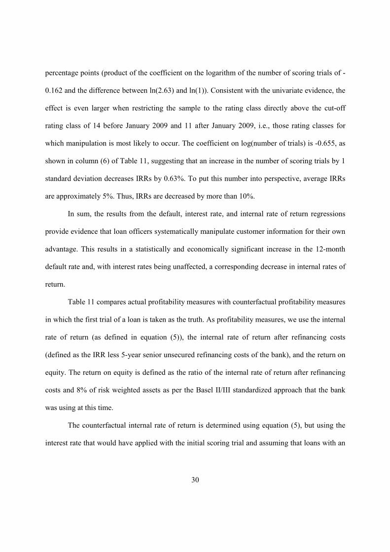
percentage points (product of the coefficient on the logarithm of the number of scoring trials of -

0.162 and the difference between ln(2.63) and ln(1)). Consistent with the univariate evidence, the

effect is even larger when restricting the sample to the rating class directly above the cut-off

rating class of 14 before January 2009 and 11 after January 2009, i.e., those rating classes for

which manipulation is most likely to occur. The coefficient on log(number of trials) is -0.655, as

shown in column (6) of Table 11, suggesting that an increase in the number of scoring trials by 1

standard deviation decreases IRRs by 0.63%. To put this number into perspective, average IRRs

are approximately 5%. Thus, IRRs are decreased by more than 10%.

In sum, the results from the default, interest rate, and internal rate of return regressions

provide evidence that loan officers systematically manipulate customer information for their own

advantage. This results in a statistically and economically significant increase in the 12-month

default rate and, with interest rates being unaffected, a corresponding decrease in internal rates of

return.

Table 11 compares actual profitability measures with counterfactual profitability measures

in which the first trial of a loan is taken as the truth. As profitability measures, we use the internal

rate of return (as defined in equation (5)), the internal rate of return after refinancing costs

(defined as the IRR less 5-year senior unsecured refinancing costs of the bank), and the return on

equity. The return on equity is defined as the ratio of the internal rate of return after refinancing

costs and 8% of risk weighted assets as per the Basel II/III standardized approach that the bank

was using at this time.

The counterfactual internal rate of return is determined using equation (5), but using the

interest rate that would have applied with the initial scoring trial and assuming that loans with an

31

initial scoring trial worse than the cut-off are rejected by the loan officer. The counterfactual IRR

after refinancing costs and the counterfactual RoE are determined accordingly.

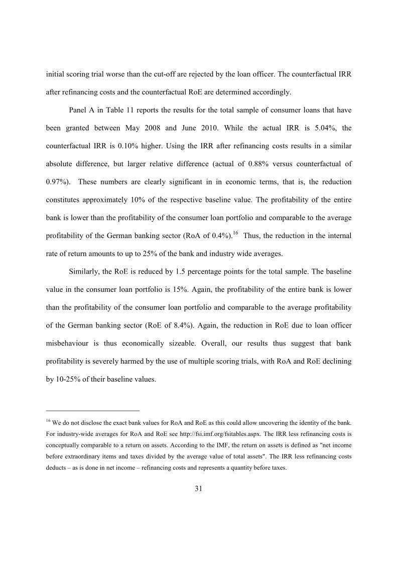
Panel A in Table 11 reports the results for the total sample of consumer loans that have

been granted between May 2008 and June 2010. While the actual IRR is 5.04%, the

counterfactual IRR is 0.10% higher. Using the IRR after refinancing costs results in a similar

absolute difference, but larger relative difference (actual of 0.88% versus counterfactual of

0.97%). These numbers are clearly significant in in economic terms, that is, the reduction

constitutes approximately 10% of the respective baseline value. The profitability of the entire

bank is lower than the profitability of the consumer loan portfolio and comparable to the average

profitability of the German banking sector (RoA of 0.4%).16

Thus, the reduction in the internal

rate of return amounts to up to 25% of the bank and industry wide averages.

Similarly, the RoE is reduced by 1.5 percentage points for the total sample. The baseline

value in the consumer loan portfolio is 15%. Again, the profitability of the entire bank is lower

than the profitability of the consumer loan portfolio and comparable to the average profitability

of the German banking sector (RoE of 8.4%). Again, the reduction in RoE due to loan officer

misbehaviour is thus economically sizeable. Overall, our results thus suggest that bank

profitability is severely harmed by the use of multiple scoring trials, with RoA and RoE declining

by 10-25% of their baseline values.

16 We do not disclose the exact bank values for RoA and RoE as this could allow uncovering the identity of the bank.

For industry-wide averages for RoA and RoE see http://fsi.imf.org/fsitables.aspx. The IRR less refinancing costs is

conceptually comparable to a return on assets. According to the IMF, the return on assets is defined as "net income

before extraordinary items and taxes divided by the average value of total assets". The IRR less refinancing costs

deducts – as is done in net income – refinancing costs and represents a quantity before taxes.

32

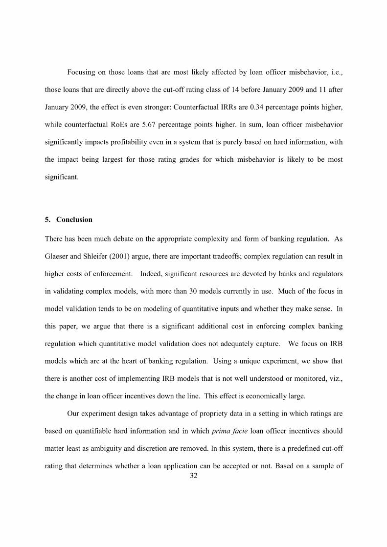
Focusing on those loans that are most likely affected by loan officer misbehavior, i.e.,

those loans that are directly above the cut-off rating class of 14 before January 2009 and 11 after

January 2009, the effect is even stronger: Counterfactual IRRs are 0.34 percentage points higher,

while counterfactual RoEs are 5.67 percentage points higher. In sum, loan officer misbehavior

significantly impacts profitability even in a system that is purely based on hard information, with

the impact being largest for those rating grades for which misbehavior is likely to be most

significant.

5. Conclusion

There has been much debate on the appropriate complexity and form of banking regulation. As

Glaeser and Shleifer (2001) argue, there are important tradeoffs; complex regulation can result in

higher costs of enforcement. Indeed, significant resources are devoted by banks and regulators

in validating complex models, with more than 30 models currently in use. Much of the focus in

model validation tends to be on modeling of quantitative inputs and whether they make sense. In

this paper, we argue that there is a significant additional cost in enforcing complex banking

regulation which quantitative model validation does not adequately capture. We focus on IRB

models which are at the heart of banking regulation. Using a unique experiment, we show that

there is another cost of implementing IRB models that is not well understood or monitored, viz.,

the change in loan officer incentives down the line. This effect is economically large.

Our experiment design takes advantage of propriety data in a setting in which ratings are

based on quantifiable hard information and in which prima facie loan officer incentives should

matter least as ambiguity and discretion are removed. In this system, there is a predefined cut-off

rating that determines whether a loan application can be accepted or not. Based on a sample of

33

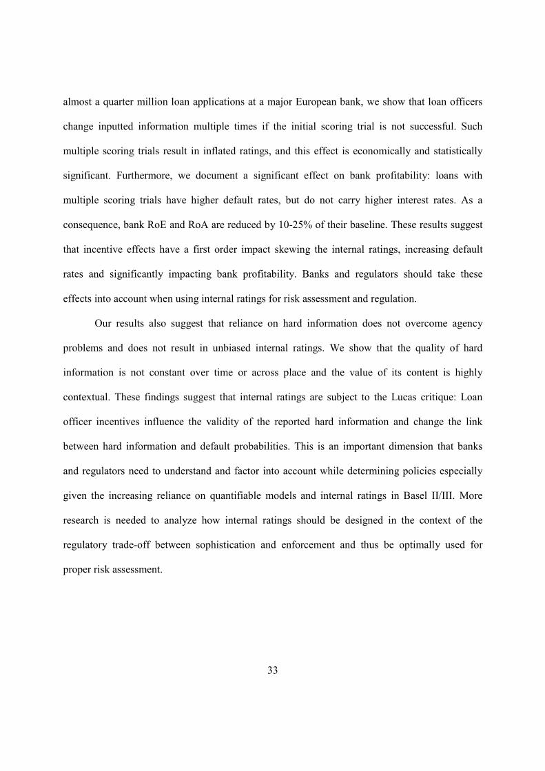
almost a quarter million loan applications at a major European bank, we show that loan officers

change inputted information multiple times if the initial scoring trial is not successful. Such

multiple scoring trials result in inflated ratings, and this effect is economically and statistically

significant. Furthermore, we document a significant effect on bank profitability: loans with

multiple scoring trials have higher default rates, but do not carry higher interest rates. As a

consequence, bank RoE and RoA are reduced by 10-25% of their baseline. These results suggest

that incentive effects have a first order impact skewing the internal ratings, increasing default

rates and significantly impacting bank profitability. Banks and regulators should take these

effects into account when using internal ratings for risk assessment and regulation.

Our results also suggest that reliance on hard information does not overcome agency

problems and does not result in unbiased internal ratings. We show that the quality of hard

information is not constant over time or across place and the value of its content is highly

contextual. These findings suggest that internal ratings are subject to the Lucas critique: Loan

officer incentives influence the validity of the reported hard information and change the link

between hard information and default probabilities. This is an important dimension that banks

and regulators need to understand and factor into account while determining policies especially

given the increasing reliance on quantifiable models and internal ratings in Basel II/III. More

research is needed to analyze how internal ratings should be designed in the context of the

regulatory trade-off between sophistication and enforcement and thus be optimally used for

proper risk assessment.

34

References

Acharya, V., R. Engle, and D. Pierret (2014). Testing macroprudential stress tests: The risk of

regulatory risk weights," Journal of Monetary Economics 65, 36-53.

Agarwal, S. and I. Ben-David (2015): “Loan Prospecting and the Loss of Soft Information,”

Working Paper.

Agarwal, S. and Hauswald, R. (2010): “Authority and Information,” Working Paper.

Akhavein, J., W.S. Frame, and L.J. White (2005): "The diffusion of financial innovations: An

examination of the adoption of small business credit scoring by large banking organizations,"

Journal of Business 78(2), 577-596.

Allen, L., G. DeLong, and A. Saunders (2004): "Issues in credit risk modeling of retail markets,"

Journal of Banking & Finance 28, 727-752.

Altman, E.I., and A. Saunders (1998): "Credit risk measurement: Developments over the last 20

years," Journal of Banking & Finance 21, 1721-1742.

Andersen, B. E. (1970): “Asymptotic Properties of Conditional Maximum-likelihood

Estimators," Journal of the Royal Statistical Society, 32(2), 283-301.

Basel Committee on Banking Supervision (2006): "International convergence of capital

measurement and capital standards – A revised framework," Bank for International Settlements,

Basel, Switzerland.

Basel Committee on Banking Supervision (2011): " Basel III: A global regulatory framework for

more resilient banks and banking systems – revised version June 2011," Bank for International

Settlements, Basel, Switzerland.

Behn, M., R. Haselmann, and V. Vig (2014): "The Limits of Model-Based Regulation," Working

Paper.

35

Berg, T. (2015): “Playing the Devil’s Advocate: The Causal Effect of Risk Management on Loan

Quality, Review of Financial Studies 28(12), 3367-3406.

Berger, A. N., N. H. Miller, M. A. Petersen, R. G. Rajan, and J. C. Stein (2005): “Does Function

Follow Organizational Form? Evidence from Lending Practices of Large and Small Banks,"

Journal of Financial Economics, 76, 237-269.

Chamberlain, G. A. (1980): “Analysis of Covariance with Qualitative Data," Review of Economic

Studies, 47, 225-238.

Cole, S., M. Kanz and L. Klapper (2015): “Incentivizing Calculated Risk Taking: Evidence from

a Series of Experiments with Commercial Bank Loan Officers,” The Journal of Finance 70(2),

537-575.

Garmaise, M.J. (2015): "Borrower Misreporting and Loan Performance," The Journal of Finance

70(1), 449-485.

Glaser, E. J., and A. Shleifer (2001): “A Reason for Quantity Regulation,” American Economic

Review, 91(2),431-435.

Hertzberg, A., J. M. Liberti, and D. Paravisini (2010): “Information and Incentives Inside a Firm:

Evidence from Loan Officer Rotation," Journal of Finance, 65(3), 795-828.

Imbens, G.W. and T. Lemieux (2008): “Regression discontinuity designs,” Journal of

Econometrics, 142, 615-635.

Keys, B. J., T. K. Mukherjee, A. Seru and V. Vig (2010): “Did Securitization Lead to Lax

Screening? Evidence from Subprime Loans," Quarterly Journal of Economics, 125(1), 307-362.

Liberti, J. M., and A. R. Mian (2009): “Estimating the Effect of Hierarchies on Information Use,"

Review of Financial Studies, 22(10), 4057-4090.

36

McCrary, J. (2008): "Manipulation of the running variable in the regression discontinuity design:

A density test," Journal of Econometrics, 142(2), 698-714.

Neyman, J., and E. Scott (1948): “Consistent Estimates Based on Partially Consistent

Observations," Econometrica, 16, 1-32.

Paravisini, A., and A. Schoar (2015): "The incentive effect of Scores: Randomized evidence from

credit committees," Working Paper, 2015.

Puri, M., J. Rocholl, and S. Steffen (2011): “Global retail lending in the aftermath of the US

financial crisis: Distinguishing between supply and demand effects," Journal of Financial

Economics, 100(3), 556-578.

Rajan, U., A. Seru, and V. Vig (2015): "The Failure of Models that Predict Failure: Distance,

Incentives, and Defaults," Journal of Financial Economics 115(2), 237-260.

Roberts, M.R. and T.M. Whited (2012): “Endogeneity in Empirical Corporate Finance,“ Simon

School Working Paper No. FR 11-29.

Stein, J. C. (2002): “Information Production and Capital Allocation: Decentralized versus

Hierarchical Firms," Journal of Finance, 57(5), 1891-1922.

Udell, G. F. (1989): “Loan Quality, Commercial Loan Review and Loan Officer Contracting,"

Journal of Banking & Finance, 13, 367-382.

Wooldridge, J. M. (2002): "Econometric Analysis of Cross Section and Panel Data." The MIT

Press, Cambridge, Massachusetts.

Thistlewaite, D., and D. Campbell, (1960): “Regression-discontinuity analysis: an alternative to

the ex-post facto experiment,” Journal of Educational Psychology, 51, 309-31.

37

Figure 1: Accepted loans by rating category

This figure compares the number of scoring trials for each loan that is accepted in each rating class for the periods before and after

January 2009.

Figure 2: Loan applications by rating category

This figure compares the number of scoring trials for each loan application based on the initial rating class for the periods before and

after January 2009.

38

Figure 3: Is Manipulation Widespread?

This figure shows the histogram of the average number of scoring trials per loan officer.

Figure 4: End-of-year effect?

This figure depicts the end-of-year manipulation effect. The vertical axis depicts the percentage of manipulations. Manipulation is

defined as (Number of loan applications where the initial scoring trial is worse than the cut-off and the final scoring trial is better than

the cut-off) divided by (Number of loan applications where the initial scoring trial is worse than the cut-off). The horizontal axis

depicts the month-of-the-year. The lines "High success rate" ("Low success rate") refer to averages of all loan officers with a success

rate of lower (higher) than 50 percent over the preceeding 9 months. The success rate is measured as loans granted divided by total

loan applications handled.

39

Table 1: Explanation of variables

Name Description

Inference and dependent variables

Cutoff Dummy variable equal to one if the internal rating is worse than the cutoff rating and zero otherwise. Only loan applications with an internal rating equal or above the cutoff rating can be accepted, loan applications with ratings below the cutoff are rejected.

Number of scoring trials Number of distinct scoring trials for a loan application.

Default rate 12 months Dummy variable equal to 1 if a loan has defaulted during the first 12 months after origination.

Manipulation (0/1) Dummy equal to one if the initial scoring trial is worse than the cut-off and the final scoring trial is better than the cut-off.

Customer characteristics

Internal rating Internal rating on a continuous scale ranging from 0.5 (best) to 24.5 (worst). The bank groups this continuous variable into 24 rating

classes ranging from 1 (best) to 24 (worst). The internal rating is based on the financial score, the socio-demographic score, the account score, the loan score and the SCHUFA score. These scores are consolidated into one overall score and calibrated to historical

default experience. Each internal rating is associated with a default probability for the borrower.

Probability of default Probability of default based on the internal rating system. The probability of default is calibrated to past default experience.

Financial score Internal score based on income, costs, assets, and liabilities of the borrower. A higher score implies a lower probability of default.

Socio-demographic score Internal score based on socio-demographic data (e.g. age, sex, etc.). A higher score implies a lower probability of default.

Account score Internal score based on the past account activity of the borrower. A higher score implies a lower probability of default.

Loan score Internal score based on the history of past loans with the same borrower. A higher score implies a lower probability of default.

Schufa score External score similar to the FICO score in the U.S. A higher score implies a lower probability of default.

Relationship customer Dummy variable equal to 1 if the customer had a checking account or a current loan with the bank before the loan application.

Age Age of borrower. If a loan application has several borrowers, e.g., husband and wife, the average age is used.

Assets Total assets of the borrower in Euro. If a loan application has several borrowers, e.g., husband and wife, then the combined assets are

used.

Liabilities Total liabilities of the borrower in Euro. If a loan application has several borrowers, e.g., husband and wife, then the combined

liabilities are used.

Income Monthly net income of the borrower in Euro. If a loan application has several borrowers, e.g., husband and wife, then the combined

income is used. The income includes wages as well as capital income and other income.

Costs Monthly net costs of the borrower in Euro. If a loan application has several borrowers, e.g., husband and wife, then the combined

costs are used. The costs include cost of living, rents and costs for existing loans.

Loan characteristics

Loan amount Loan amount in EUR.

Number of borrowers Number of borrowers, usually equal to one.

Risk weight (RW) Basel II IRB (internal-rating based) risk weight. During the period under study, the bank does not use internal ratings for consumer

loans for regulatory purposes. The risk weights reported here are risk weights that would apply if the bank would use the IRB approach for regulatory puroses.

Accepted by bank Dummy variable equal to one if the loan application is accepted by the bank, i.e. an offer is made to the customer.

Accepted by bank and customer Dummy variable equal to one if the loan application is accepted by the bank and the customer.

Loan officer characteristics

3M average number of trials per loan application

The average number of trials per loan application over the previous three months, calculated on loan officer level.

3M absolute number of trials The absolute number of scoring trials over the previous three months, calculated on loan officer level.

Success rate 3M Success rate of the loan officer over the month preceding the current month. The success rate is measured as loans granted divided by

total loan applications handled. Accepted loans are loans which were accepted by the bank and the borrower, i.e. where a loan contract was signed.

Other variables

Status Status of a scoring trial. The status can be either 'automatically rejected' if the internal rating is worse than the cutoff rating, 'manually

rejected' if the loan application is manually rejected by the loan officer and 'accepted' if the loan application is accepted by the bank and customer.

Month-of-year Month of year coded as 1 (January) through 12 (December)

40

Table 2: Descriptive statistics

This table presents summary statistics for the sample of loan applications between May 2008 and June 2010. Panel A presents summary

statistics on the loan application level based on the last scoring trial for each loan application, Panel B on the scoring trial level and

Panel C on the loan officer level. E.g. Panel A shows that 13% of the loan applications do not pass the cut-off rating based on the last

scoring trial while Panel B shows that 20% do not pass the cut-off rating based on all scoring trials. For variable definitions see Table 1.

Unit N Mean Stddev Median Min Max

Panel A: Loan applications


Number of scoring trials 242,011 1.83 1.63 1.00 1.00 69.00

Change in internal rating 242,011 -0.10 0.84 0.00 -14.65 12.34

Cutoff Dummy (0/1) 242,011 0.13 0.33 0.00 0.00 1.00

Default rate 12 months Dummy (0/1) 116,969 0.025 0.156 0.00 0.00 0.00

Customer characteristics

Internal Rating Number (1=Best, 24=Worst) 242,011 8.40 3.99 8.00 1.00 24.00

Probability of default (PD) 242,011 2.40% 6.46% 0.78% 0.01% 93.93%

Relationship customer Dummy (0/1) 242,011 0.63 0.48 1.00 0.00 1.00

Age Years 242,011 45.24 13.32 44.00 18.00 109.00

Net income per month EUR 242,011 2,665 5,208 2,321 300 2,300,000

Loan characteristics

Loan amount EUR 242,011 13,700 10,665 10,000 2,000 50,000

Number of borrowers 242,011 1.34 0.47 1.00 1.00 2.00

Risk weight (RW) 242,011 0.55 0.29 0.54 0.06 1.59

Accepted by bank Dummy (0/1) 242,011 0.70 0.46 1.00 0.00 1.00

Accepted by bank and customer Dummy (0/1) 242,011 0.48 0.50 0.00 0.00 1.00

Panel B: Scoring Trials


Cutoff Dummy (0/1) 442,255 0.20 0.40 0.00 0.00 1.00

Additional trial Dummy (0/1) 442,255 0.45 0.50 0.00 0.00 1.00

Panel C: Loan officers

Aggregate statistics

Number of scoring trials 442,255 78.50 95.79 43.00 1.00 974.00

Number of distinct loan applications 242,011 42.96 47.80 25.00 1.00 390.00

Number of accepted loans 116,969 20.78 23.93 12.00 0.00 207.00

Success Rate 3M % 242,011 45.85 22.01 47.53 0.00 100.00

41

Table 3: Mapping of internal rating to probability of default (PD) estimates

This table presents a mapping of internal ratings to probability of default estimates. Column (1) depicts the 24 internal rating classes,

column (2) shows the average probability of default that the banks assigns to borrowers in this rating class, column (3) shows the

absolute reduction in the probability of default when increasing the rating class by 1 notch, column (4) shows the relative reduction in

the probability of default when increasing the rating class by 1 notch. For variable definitions see Table 1.

(1) (2) (3) (4)

Rating class Mean(PD)

Reduction in PD per 1 notch

change in internal rating class

(absolute)

Reduction in PD per 1 notch

change in internal rating

(relative)

1 (best) 0.016% 0.034% -68%

2 0.050% 0.034% -40%

3 0.084% 0.053% -39%

4 0.137% 0.084% -38%

5 0.221% 0.124% -36%

6 0.345% 0.174% -34%

7 0.519% 0.243% -32%

8 0.762% 0.361% -32%

9 1.123% 0.487% -30%

10 1.610% 0.665% -29%

11 2.275% 0.789% -26%

12 3.064% 1.033% -25%

13 4.097% 1.288% -24%

14 5.385% 1.383% -20%

15 6.768% 1.733% -20%

16 8.501% 2.005% -19%

17 10.506% 2.488% -19%

18 12.994% 3.016% -19%

19 16.010% 3.780% -19%

20 19.790% 4.573% -19%

21 24.363% 5.356% -18%

22 29.719% 6.363% -18%

23 36.082% 17.119% -32%

24 (worst) 53.201%

42

Table 4: Example

This table presents the scoring trials for one single consumer loan originated on May, 04th, 2009. Changes in input parameters are highlighted in bold. For variable definitions see

Table 1. Ratings with an internal rating class of 11 or better can be accepted.

Trial

No. Date

Internal

rating

class Cutoff

Loan

amount Assets Liabilities Income Costs Status

1 4 May 2009 4:03:24 PM 12 1 4,000 1,800 23,000 1,900 1,080 Automatically rejected


3 4 May 2009 4:15:00 PM 11 0 4,000 1,800 10,000 1,950 1,080 Manually rejected


5 4 May 2009 4:16:23 PM 11 0 4,000 1,800 10,000 1,950 1,080 Accepted

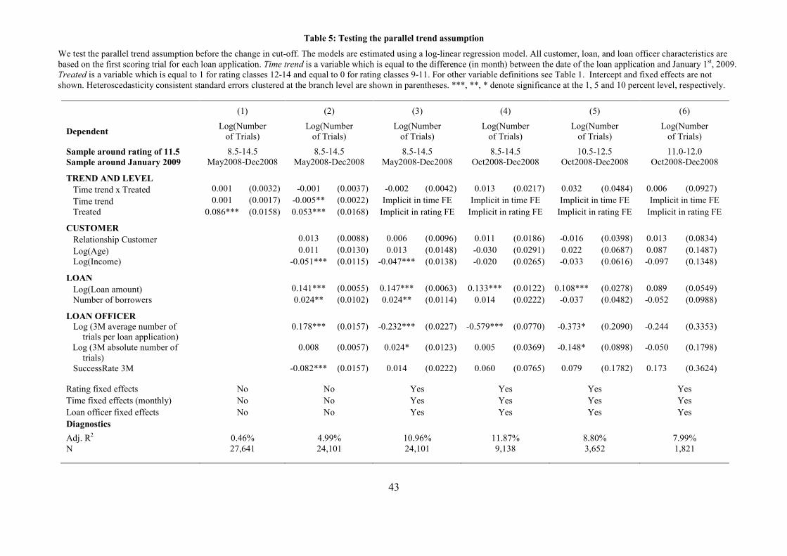
43

Table 5: Testing the parallel trend assumption

We test the parallel trend assumption before the change in cut-off. The models are estimated using a log-linear regression model. All customer, loan, and loan officer characteristics are

based on the first scoring trial for each loan application. Time trend is a variable which is equal to the difference (in month) between the date of the loan application and January 1st, 2009.

Treated is a variable which is equal to 1 for rating classes 12-14 and equal to 0 for rating classes 9-11. For other variable definitions see Table 1. Intercept and fixed effects are not

shown. Heteroscedasticity consistent standard errors clustered at the branch level are shown in parentheses. ***, **, * denote significance at the 1, 5 and 10 percent level, respectively.

(1) (2) (3) (4) (5) (6)

Dependent Log(Number

of Trials)

Log(Number

of Trials)

Log(Number

of Trials)

Log(Number

of Trials)

Log(Number

of Trials)

Log(Number

of Trials)

Sample around rating of 11.5

Sample around January 2009

8.5-14.5

May2008-Dec2008

8.5-14.5

May2008-Dec2008

8.5-14.5

May2008-Dec2008

8.5-14.5

Oct2008-Dec2008

10.5-12.5

Oct2008-Dec2008

11.0-12.0

Oct2008-Dec2008

TREND AND LEVEL

Time trend x Treated 0.001 (0.0032) -0.001 (0.0037) -0.002 (0.0042) 0.013 (0.0217) 0.032 (0.0484) 0.006 (0.0927)

Time trend 0.001 (0.0017) -0.005** (0.0022) Implicit in time FE Implicit in time FE Implicit in time FE Implicit in time FE

Treated 0.086*** (0.0158) 0.053*** (0.0168) Implicit in rating FE Implicit in rating FE Implicit in rating FE Implicit in rating FE

CUSTOMER

Relationship Customer 0.013 (0.0088) 0.006 (0.0096) 0.011 (0.0186) -0.016 (0.0398) 0.013 (0.0834)

Log(Age) 0.011 (0.0130) 0.013 (0.0148) -0.030 (0.0291) 0.022 (0.0687) 0.087 (0.1487)

Log(Income) -0.051*** (0.0115) -0.047*** (0.0138) -0.020 (0.0265) -0.033 (0.0616) -0.097 (0.1348)

LOAN

Log(Loan amount) 0.141*** (0.0055) 0.147*** (0.0063) 0.133*** (0.0122) 0.108*** (0.0278) 0.089 (0.0549)

Number of borrowers 0.024** (0.0102) 0.024** (0.0114) 0.014 (0.0222) -0.037 (0.0482) -0.052 (0.0988)

LOAN OFFICER

Log (3M average number of

trials per loan application)

0.178*** (0.0157) -0.232*** (0.0227) -0.579*** (0.0770) -0.373* (0.2090) -0.244 (0.3353)

Log (3M absolute number of

trials)

0.008 (0.0057) 0.024* (0.0123) 0.005 (0.0369) -0.148* (0.0898) -0.050 (0.1798)

SuccessRate 3M -0.082*** (0.0157) 0.014 (0.0222) 0.060 (0.0765) 0.079 (0.1782) 0.173 (0.3624)

Rating fixed effects No No Yes Yes Yes Yes

Time fixed effects (monthly) No No Yes Yes Yes Yes

Loan officer fixed effects No No Yes Yes Yes Yes

Diagnostics

Adj. R2 0.46% 4.99% 10.96% 11.87% 8.80% 7.99%

N 27,641 24,101 24,101 9,138 3,652 1,821

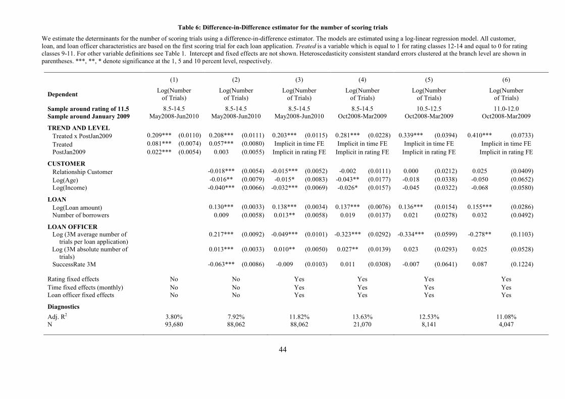
44

Table 6: Difference-in-Difference estimator for the number of scoring trials

We estimate the determinants for the number of scoring trials using a difference-in-difference estimator. The models are estimated using a log-linear regression model. All customer,

loan, and loan officer characteristics are based on the first scoring trial for each loan application. Treated is a variable which is equal to 1 for rating classes 12-14 and equal to 0 for rating

classes 9-11. For other variable definitions see Table 1. Intercept and fixed effects are not shown. Heteroscedasticity consistent standard errors clustered at the branch level are shown in

parentheses. ***, **, * denote significance at the 1, 5 and 10 percent level, respectively.

(1) (2) (3) (4) (5) (6)

Dependent Log(Number

of Trials)

Log(Number

of Trials)

Log(Number

of Trials)

Log(Number

of Trials)

Log(Number

of Trials)

Log(Number

of Trials)



8.5-14.5

May2008-Jun2010

8.5-14.5

May2008-Jun2010

8.5-14.5

May2008-Jun2010

8.5-14.5

Oct2008-Mar2009

10.5-12.5

Oct2008-Mar2009

11.0-12.0

Oct2008-Mar2009

TREND AND LEVEL

Treated x PostJan2009 0.209*** (0.0110) 0.208*** (0.0111) 0.203*** (0.0115) 0.281*** (0.0228) 0.339*** (0.0394) 0.410*** (0.0733)

Treated 0.081*** (0.0074) 0.057*** (0.0080) Implicit in time FE Implicit in time FE Implicit in time FE Implicit in time FE

PostJan2009 0.022*** (0.0054) 0.003 (0.0055) Implicit in rating FE Implicit in rating FE Implicit in rating FE Implicit in rating FE

CUSTOMER

Relationship Customer -0.018*** (0.0054) -0.015*** (0.0052) -0.002 (0.0111) 0.000 (0.0212) 0.025 (0.0409)

Log(Age) -0.016** (0.0079) -0.015* (0.0083) -0.043** (0.0177) -0.018 (0.0338) -0.050 (0.0652)

Log(Income) -0.040*** (0.0066) -0.032*** (0.0069) -0.026* (0.0157) -0.045 (0.0322) -0.068 (0.0580)

LOAN

Log(Loan amount) 0.130*** (0.0033) 0.138*** (0.0034) 0.137*** (0.0076) 0.136*** (0.0154) 0.155*** (0.0286)

Number of borrowers 0.009 (0.0058) 0.013** (0.0058) 0.019 (0.0137) 0.021 (0.0278) 0.032 (0.0492)

LOAN OFFICER



0.217*** (0.0092) -0.049*** (0.0101) -0.323*** (0.0292) -0.334*** (0.0599) -0.278** (0.1103)

Log (3M absolute number of

trials)

0.013*** (0.0033) 0.010** (0.0050) 0.027** (0.0139) 0.023 (0.0293) 0.025 (0.0528)

SuccessRate 3M -0.063*** (0.0086) -0.009 (0.0103) 0.011 (0.0308) -0.007 (0.0641) 0.087 (0.1224)




Diagnostics

Adj. R2 3.80% 7.92% 11.82% 13.63% 12.53% 11.08%

N 93,680 88,062 88,062 21,070 8,141 4,047

45

Table 7: Difference-in-Difference estimator for the change in rating, change in probability of default estimate, change in risk-weighted assets

We estimate the determinants for the change in various variables from the initial to the final scoring trial using a difference-in-difference estimator. Column (1) provides results for

changes in the rating, column (2) for the change in the probability of default estimate, and column (3) for the change in the Basel II risk weight if the internal rating based approach would

have been used. The models are estimated using a linear regression model. All customer, loan, and loan officer characteristics are based on the first scoring trial for each loan application.

Treated is a variable which is equal to 1 for rating classes 12-14 and equal to 0 for rating classes 9-11. For other variable definitions see Table 1. Intercept and fixed effects are not

shown. Heteroscedasticity consistent standard errors clustered at the branch level are shown in parentheses. ***, **, * denote significance at the 1, 5 and 10 percent level, respectively.

(1) (2) (3)

Dependent

Change in rating

from initial to

final scoring trial

Change in the probability of default

estimate from initial to final scoring trial,

ln(PDfinal trial

)-ln(PDinital trial

)

Change in Basel IRB risk weight

from initial to final scoring trial

ln(RWfinal trial

)-ln(RWinitial trial

)



8.5-14.5

May2008-Jun2010

8.5-14.5

Oct2008-Mar2009

10.5-12.5

Oct2008-Mar2009

TREND AND LEVEL

Treated x PostJan2009 -0.265*** (0.0134) -0.086*** (0.0046) -0.027*** (0.0015)

Treated Implicit in time FE Implicit in time FE Implicit in time FE

PostJan2009 Implicit in rating FE Implicit in rating FE Implicit in rating FE

CUSTOMER

Relationship Customer 0.071*** (0.0063) 0.023*** (0.0023) 0.008*** (0.0008)

Log(Age) 0.010 (0.0099) 0.002 (0.0037) 0.003* (0.0013)

Log(Income) 0.058*** (0.0080) 0.019*** (0.0030) 0.006*** (0.0011)

LOAN

Log(Loan amount) -0.086*** (0.0037) -0.029*** (0.0014) -0.012*** (0.0005)

Number of borrowers 0.042*** (0.0072) 0.015*** (0.0027) 0.005*** (0.0010)

LOAN OFFICER



0.020* (0.0109) 0.007* (0.0040) 0.003** (0.0015)

Log (3M absolute number of trials) -0.003 (0.0054) -0.001 (0.0020) -0.001 (0.0007)

SuccessRate 3M 0.005 (0.0109) 0.002 (0.0039) 0.000 (0.0015)

Rating fixed effects Yes Yes Yes

Time fixed effects (monthly) Yes Yes Yes

Loan officer fixed effects Yes Yes Yes

Diagnostics

Adj. R2 5.98% 4.72% 4.34%

N 88,062 88,062 88,062

46

Table 8: Multivariate results for the number of scoring trials – Regression discontinuity

This table reports a McCrary density test and regression discontinuity estimates. Panel I reports the results from the McCrary test for

the manipulation of the running variable. Panel II tests for the discontinuity in the number of scoring trials at the cut-off rating using

seventh-order polynomials and local linear regression on either side of the cutoff using a log-linear regression model. Column (A)

presents results for the period before January 2009, column (B) presents the results for the period after January 2009. Columns (C1)

and (D1) report results for the estimate of the discontinuity, columns (C2) and (D2) report robust standard errors, columns (C3) and

(D3) report the number of observations and columns (C4) and (D4) report the R-squared. “Without Covariates” denotes regressions

without any covariates beyond the initial rating, “With Covariates” denotes regressions which include customer, client and loan officer

characteristics (which are not shown for reasons of brevity). Columns (C1) and (D1) report the estimate of the discontinuity in the

density of the internal rating at the cutoff rating, columns (C2) and (D2) report the respective standard errors. ***, **, * denotes

significance at the 1, 5 and 10 percent level, respectively.

(A) Before January 2009

(B) After January 2009

Panel I: McCrary test for manipulation of the running variable at the cutoff rating

(A1) (A2) (B1) (B2)

Discontinuity

at rating of

14.5 (SE)

Discontinuity

at rating of

11.5 (SE)

Initial rating 0.084 (0.1976)

-0.024 (0.0711)

Final rating -0.523*** (0.1837)

-0.828*** (0.0684)

Panel II: Test for discontinuity in the number of scoring trials at the cutoff rating

(C1) (C2) (C3) (C4)

(D1) (D2) (D3) (D4)

Method

Initial rating

> 14.5 (β) (SE) Observations Adj. R2

Initial rating

> 11.5 (β) t-stat Observations Adj. R2

Method: Polynomials (all rating classes)

without covariates 0.334*** (0.0527) 70,330 5.68%

0.266*** (0.0214) 171,681 5.86%

with covariates 0.346*** (0.0539) 61,065 14.23%

0.265*** (0.0212) 165,692 13.02%

Method: Local linear regression (+/- 1 notch around cut-off)

without covariates 0.318*** (0.0449) 3,613 5.89%

0.274*** (0.0176) 25,433 4.77%

with covariates 0.358*** (0.0863) 3,148 14.49%

0.268*** (0.0200) 24,621 11.71%

47

Table 9: Default rates, interest rates, and internal rate of return by rating class and number of scoring trials

This table presents default rates (Panel A), interest rates (Panel B), and internal rates of return (Panel C) by rating class and by number

of scoring trials before and after the change in the cutoff rating in January 2009. Internal rates of return are calculated as IRR =

interest rate – default rate x loss given default – operating cost, using a 40% loss given default assumption and a 3% operating cost

assumption. The rating class is based on the final rating for each loan. An internal rating of ‘1’ is the best rating, an internal rating

class of ‘14’ is the worst rating for which loans could be accepted before January 2009, an internal rating class of ‘11’ is the worst

rating for which loans could be accepted after January 2009. In each Panel, column A shows results before January 2009 and column

B shows results after January 2009. Column (A1) and (B1) provide results for loans with one or two scoring trials, Column (A2) and

(B2) provide results for loans with more than two scoring trials, columns (A3) and (B3) provide results for the difference between

loans with one or two and more than two scoring trials and columns (A4) and (B4) provide the respective p-values based on an exact

Fisher test (Panel A) and a t-test (Panel B and C). For brevity, the number of observations is not shown. ***, **, * denotes

significance at the 1, 5 and 10 percent level, respectively.

Panel A: Default rates

(A)

(B)

Before January 2009

After January 2009

(A1) (A2) (A3) (A4)

(B1) (B2) (B3) (B4)

Internal Rating Class

(from last scoring trial)

Loans with

≤ 2 trials

Loans with

> 2 scoring trials Difference p-value

Loans with

≤ 2 trials

Loans with

> 2 scoring trials Difference p-value

1 0.088% 0.336% 0.248% 0.3083

0.195% 0.000% -0.195% 0.6076

2 0.147% 0.000% -0.147% 1.0000

0.144% 0.930% 0.786%* 0.0891

3 0.246% 0.000% -0.246% 1.0000

0.509% 0.402% -0.107% 1.0000

4 0.254% 0.575% 0.321% 0.4230

0.300% 0.542% 0.242% 0.3531

5 0.445% 0.365% -0.080% 1.0000

0.813% 0.153% -0.660%* 0.0798

6 0.742% 0.509% -0.233% 0.7910

0.609% 0.680% 0.071% 0.7296

7 1.174% 0.530% -0.645%* 0.0857

1.522% 1.185% -0.337% 0.2510

8 1.297% 0.931% -0.366% 0.4752

1.954% 1.729% -0.225% 0.5830

9 1.961% 2.507% 0.546% 0.3836

2.769% 2.602% -0.167% 0.7516

10 2.731% 2.370% -0.360% 0.6879

3.910% 4.311% 0.401% 0.4735

11 4.745% 5.828% 1.083% 0.2166

7.829% 10.113% 2.285%*** 0.0001

12 5.201% 5.687% 0.486% 0.6117

13 7.759% 6.349% -1.409% 0.3644

14 7.091% 12.148% 5.057%*** 0.0011

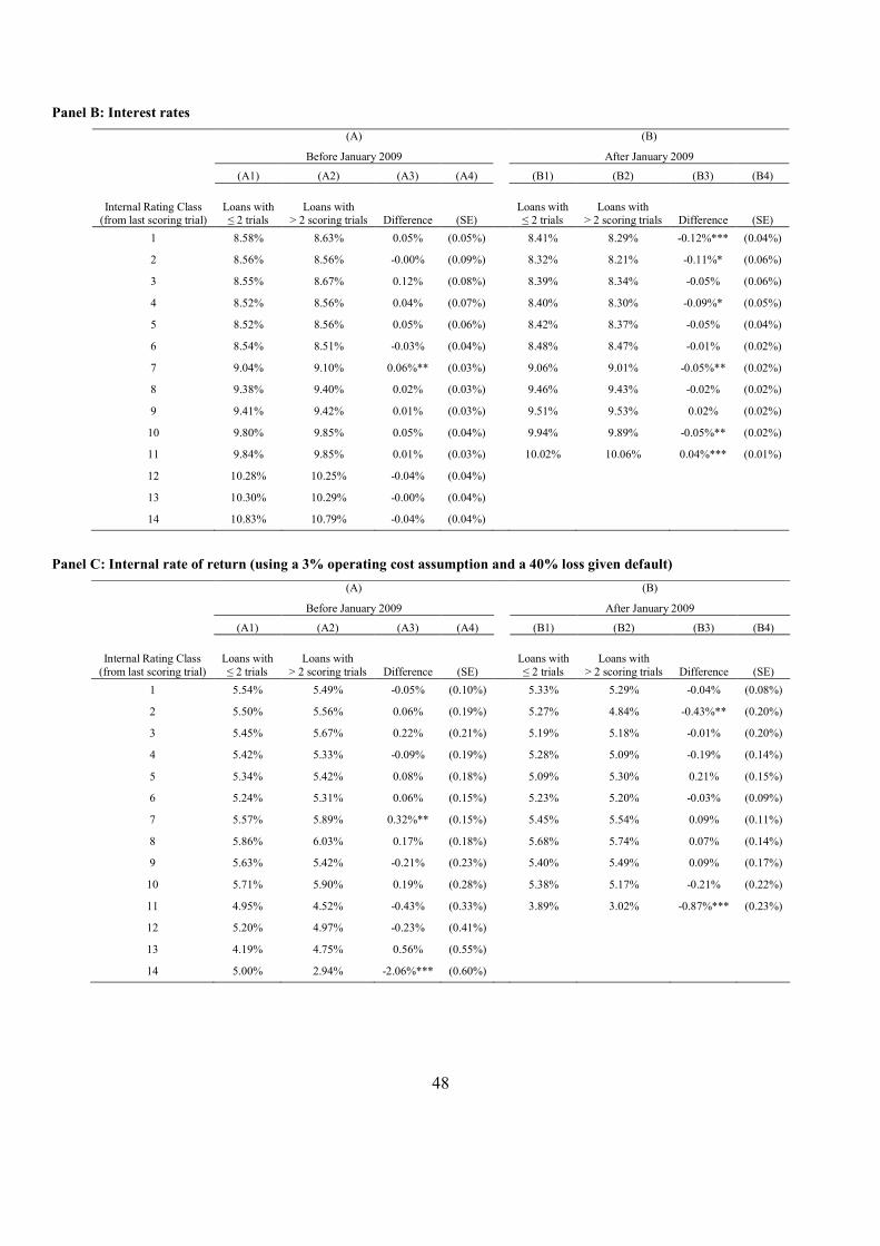
48

Panel B: Interest rates

(A) (B)

Before January 2009

After January 2009

(A1) (A2) (A3) (A4)

(B1) (B2) (B3) (B4)

Internal Rating Class (from last scoring trial)

Loans with ≤ 2 trials

Loans with > 2 scoring trials Difference (SE)

Loans with ≤ 2 trials

Loans with > 2 scoring trials Difference (SE)

1 8.58% 8.63% 0.05% (0.05%) 8.41% 8.29% -0.12%*** (0.04%)

2 8.56% 8.56% -0.00% (0.09%) 8.32% 8.21% -0.11%* (0.06%)

3 8.55% 8.67% 0.12% (0.08%) 8.39% 8.34% -0.05% (0.06%)

4 8.52% 8.56% 0.04% (0.07%) 8.40% 8.30% -0.09%* (0.05%)

5 8.52% 8.56% 0.05% (0.06%) 8.42% 8.37% -0.05% (0.04%)

6 8.54% 8.51% -0.03% (0.04%) 8.48% 8.47% -0.01% (0.02%)

7 9.04% 9.10% 0.06%** (0.03%) 9.06% 9.01% -0.05%** (0.02%)

8 9.38% 9.40% 0.02% (0.03%) 9.46% 9.43% -0.02% (0.02%)

9 9.41% 9.42% 0.01% (0.03%) 9.51% 9.53% 0.02% (0.02%)

10 9.80% 9.85% 0.05% (0.04%) 9.94% 9.89% -0.05%** (0.02%)

11 9.84% 9.85% 0.01% (0.03%) 10.02% 10.06% 0.04%*** (0.01%)

12 10.28% 10.25% -0.04% (0.04%)

13 10.30% 10.29% -0.00% (0.04%)

14 10.83% 10.79% -0.04% (0.04%)

Panel C: Internal rate of return (using a 3% operating cost assumption and a 40% loss given default)

(A) (B)

Before January 2009

After January 2009

(A1) (A2) (A3) (A4)

(B1) (B2) (B3) (B4)

Internal Rating Class

(from last scoring trial)

Loans with

≤ 2 trials

Loans with

> 2 scoring trials Difference (SE)

Loans with

≤ 2 trials

Loans with

> 2 scoring trials Difference (SE)

1 5.54% 5.49% -0.05% (0.10%) 5.33% 5.29% -0.04% (0.08%)

2 5.50% 5.56% 0.06% (0.19%) 5.27% 4.84% -0.43%** (0.20%)

3 5.45% 5.67% 0.22% (0.21%) 5.19% 5.18% -0.01% (0.20%)

4 5.42% 5.33% -0.09% (0.19%) 5.28% 5.09% -0.19% (0.14%)

5 5.34% 5.42% 0.08% (0.18%) 5.09% 5.30% 0.21% (0.15%)

6 5.24% 5.31% 0.06% (0.15%) 5.23% 5.20% -0.03% (0.09%)

7 5.57% 5.89% 0.32%** (0.15%) 5.45% 5.54% 0.09% (0.11%)

8 5.86% 6.03% 0.17% (0.18%) 5.68% 5.74% 0.07% (0.14%)

9 5.63% 5.42% -0.21% (0.23%) 5.40% 5.49% 0.09% (0.17%)

10 5.71% 5.90% 0.19% (0.28%) 5.38% 5.17% -0.21% (0.22%)

11 4.95% 4.52% -0.43% (0.33%) 3.89% 3.02% -0.87%*** (0.23%)

12 5.20% 4.97% -0.23% (0.41%)

13 4.19% 4.75% 0.56% (0.55%)

14 5.00% 2.94% -2.06%*** (0.60%)

49

Table 10: Multivariate results for the default rate, interest rates, and the internal rate of return

This table provides results of a regression of the default rate dummy (columns (1)-(3)), the interest rate (column (4)), and the internal rate of return (column (5) and (6)) on the logarithm of the

number of scoring trials and control variables. The default rate dummy is equal to zero if a loan defaults over the first 12 months after origination. The interest rate is the contractual interest rate

of a loan. The internal rate of return is calculated as IRR = interest rate – default rate dummy x loss given default – operating cost, using a 40% loss given default assumption and a 3%

operating cost assumption. The models are estimated using a linear probability model. For variable definitions see Table 1. Intercept and fixed effects are not shown. Heteroscedasticity

consistent standard errors clustered at the branch level are shown in parentheses. ***, **, * denote significance at the 1, 5 and 10 percent level, respectively.

(1) (2) (3) (4) (5) (6)

Dependent Default rate

12months

Default rate

12months

Default rate

12months

Interest Rate

(in Percent)

IRR

(in Percent)

IRR

(in Percent)

Sample All loans All loans All loans All loans All loans

Loans directly above cut-off

(rating of 14 until Dec2008,

rating of 11 after Dec2008)

Model Linear Linear Linear Linear Linear Linear

INCENTIVE

Log(Number of trials) 0.011*** (0.0013) 0.008*** (0.0012) 0.004*** (0.0012) 0.007 (0.0048) -0.162*** (0.047) -0.655** (0.2347)

CUSTOMER

Relationship Customer -0.048*** (0.0037) -0.032*** (0.0027) -0.039*** (0.0059) 1.249*** (0.1074) 1.834*** (0.3376)

Log(Age) -0.034*** (0.0025) -0.018*** (0.0023) 0.000 (0.0090) 0.736*** (0.0931) 3.154*** (0.6032)

Log(Income) -0.013*** (0.0018) -0.013*** (0.0019) -0.071*** (0.0073) 0.456*** (0.0751) 0.734 (0.4958)

LOAN

Log(Loan amount) 0.009*** (0.0013) 0.003*** (0.0011) -0.034*** (0.0039) -0.165*** (0.0452) -0.214 (0.2353)

Number of borrowers -0.044*** (0.0032) -0.032*** (0.0027) -0.018*** (0.0067) 1.249*** (0.1059) 2.469*** (0.4131)

LOAN OFFICER

Log (3M average number of trials per

loan application)

-0.002 (0.0026) -0.005** (0.0023) 0.003 (0.0108) 0.188** (0.0928) 1.251* (0.7247)

Log (3M absolute number of trials) 0.008*** (0.0012) 0.006*** (0.0013) -0.003 (0.0052) -0.239*** (0.0514) -0.378 (0.3312)

SuccessRate 3M 0.000 (0.0026) 0.002 (0.0025) 0.002 (0.0124) -0.066 (0.0989) -0.293 (0.8266)




Diagnostics

Adj. R2 0.17% 2.95% 7.52% 49.21% 5.78% 7.15%

N 116,969 109,787 109,787 109,787 109,787 11,431

50

Table 11: Economic impact

This table summarizes the economic impact of manipulation on the internal rate of return (IRR), risk weights and

Return on Equity (RoE). IRR is determined using the formula

IRR = interest rate – default rate x loss given default – operating cost,

where interest rate is the interest rate from the first/final scoring trial, default rate is the actual default rate, loss

given default is set to 60% and operating costs are set to 3%. Risk weights are calculated using the standardized

approach of Basel II/III for the class "other retail", i.e. a 75% risk weight. RoE is determined using the formula

RoE = (IRR – refinancing costs) / (8% x risk weighted assets),

where refinancing costs are the senior unsecured fundings costs for a maturity of 5 years of the bank at the date of

origination. Panel A reports results for all loans, Panel B restricts the sample to loans with an initial rating of +/- 2

rating grades around the cut-off. The row "Actual" uses the sample of loans that were actually granted (final trial

better than the cut-off), the rows "Counterfactual" only uses the sample of loans where the initial scoring trial was

better than the cut-off.

Panel A: All loans

IRR

IRR less

refinancing costs

(RoA) RoE

Actual: Interest rate, risk

weights, and loan decisions

based on final trial

5.04% 0.88% 14.67%

Counterfactual: Interest rate,

risk weights, and loan

decisions based on first trial

5.14% 0.97% 16.17%

Difference -0.10% -0.09% 1.50%

Panel B: Rating grade directly above (i.e., better than) the cut-off

(i.e., rating of 14 until Dec2008, rating of 11 after Dec2008)

IRR

IRR less

refinancing costs

(RoA) RoE

Actual: Interest rate, risk

weights, and loan decisions

based on final trial

3.37% -0.50% -8.33%

Counterfactual: Interest rate,

risk weights, and loan

decisions based on first trial

3.71% -0.16% -2.67%

Difference -0.34% -0.34% 5.67%

51

Appendix A: Time per trial and changes to input parameters

We analyze further determinants for default rates in Appendix Table 1. If a loan officer

uses multiple scoring trials to manipulate information, then the time between the scoring trials

should be negatively related to the default rates. In this case, the loan officer does not carefully

check or verify the existing information, but simply plays with the input parameters to change the

rating outcome. If, however, multiple scoring trials are due to the closer examination of

information or information verification from the first trial, we would expect the opposite result.

The results in column (1) show that shorter trials are indeed associated with higher default rates

and thus suggest that the loan officer does not give much care when revising the information.

Furthermore, it should be much easier for the loan officer to change information on liabilities and

costs rather than on assets and income to achieve the desired outcome. While adding assets and

income would have to be proven by respective documents, reducing liabilities and costs could be

achieved by simply ignoring certain positions. This link is tested in columns (2) to (4). The

results in column (2) show that it is indeed the change in liabilities and costs that increases

default rates, while the results in column (3) show that it is a reduction in both positions that

increases default rates. Combining the results from column (1) and column (3), the results in

column (4) show that a shorter time per trial as well as a reduction in costs and liabilities are

associated with higher default rates. These results should not be interpreted causally: Shorter

trials or changes to costs and liabilities do not cause higher default rates. Rather, incentives

created by the cut-off rule cause loan officer to use multiple, short scoring trials that are not based

on any relevant information about the client.17

17 In a further robustness test, we split the number of scoring trials into the number of short scoring trials (less than a

minute) plus the number of long scoring trials (more than a minute). Only the number of short trials is correlated

with subsequent default rates, while the while the number of long scoring trials does not show up significant in the

regression. Results are available upon request.

52

Appendix Table 1: Multivariate results for the default rate: Time per trial and changes to input parameters

We estimate the probability of default over the first 12 months after origination. The models are estimated using a linear probability model. Log(Time per Trial) denotes the time from the first to the last scoring trial

(measured in hours) divided by the number of scoring trials minus 1. This item is therefore only available for loan applications with more than one scoring trial. ∆(logAssets) [∆(logLiabilities), ∆(logIncome),

∆(logCosts)] denotes the logarithm of the assets [liabilities, income, costs] from the final scoring trial minus the logarithm of the assets [liabilities, income, costs] from the initial scoring trial. max(∆(logAssets), 0) is

equal to ∆(logAssets) if assets are increased and zero if assets are decreased while min(∆(logAssets), 0) is equal to ∆(logAssets) if assets are decreased and zero if assets are increased , the same applies to liabilities,

income and costs. For the remaining variable definitions see Table 1. Intercept and fixed effects are not shown. Heteroscedasticity consistent standard errors clustered at the branch level are shown in parentheses.

***, **, * denote significance at the 1, 5 and 10 percent level, respectively.

(1) (2) (3) (4)

Dependent Default rate 12 months Default rate 12 months Default rate 12 months Default rate 12 months

Model Linear Linear Linear Linear

INCENTIVE

Log(Number of trials) 0.010*** (0.0027) 0.004*** (0.0012) 0.004*** (0.0013) 0.010*** (0.0027) Log(Time per trial) -0.0009*** (0.0003) -0.0009*** (0.0003)

∆(logAssets) 0.000 (0.0007)

min(∆(logAssets), 0) 0.007 (0.0114) 0.003 (0.0119) max(∆(logAssets), 0) 0.001 (0.0008) 0.000 (0.0008)

∆(logLiabilities) -0.002*** (0.0005)

min(∆(logLiabilities), 0) -0.002*** (0.0006) -0.002*** (0.0006) max(∆(logLiabilities), 0) 0.000 (0.0011) 0.000 (0.0012)

∆(logIncome) -0.028 (0.0205)

min(∆(logIncome), 0) -0.038 (0.0323) -0.065* (0.0351) max(∆(logIncome), 0) -0.017 (0.0279) -0.006 (0.0291)

∆(logCosts) -0.015** (0.0063)

min(∆(logCosts), 0) -0.023*** (0.0079) -0.024*** (0.0084) max(∆(logCosts), 0) 0.004 (0.0123) 0.004 (0.0131)

CUSTOMER Relationship Customer -0.035*** (0.0037) -0.032*** (0.0027) -0.032*** (0.0027) -0.035*** (0.0037)

Log(Age) -0.023*** (0.0036) -0.018*** (0.0023) -0.018*** (0.0023) -0.023*** (0.0036) Log(Income) -0.017*** (0.0028) -0.013*** (0.0019) -0.013*** (0.0019) -0.017*** (0.0029)

LOAN

Log(Loan amount) 0.003* (0.0017) 0.003*** (0.0011) 0.003*** (0.0011) 0.004** (0.0017) Number of borrowers -0.034*** (0.0037) -0.032*** (0.0027) -0.032*** (0.0027) -0.034*** (0.0037)

LOAN OFFICER Log (3M average number of trials per loan application) -0.007* (0.0038) -0.005** (0.0023) -0.005** (0.0023) -0.007 (0.0037)

Log (3M absolute number of trials) 0.009*** (0.0021) 0.006*** (0.0013) 0.006*** (0.0013) 0.009*** (0.0021)

SuccessRate 3M -0.004 (0.0041) 0.002 (0.0025) 0.002 (0.0025) -0.004 (0.0041)

Rating fixed effects Yes Yes Yes Yes

Time fixed effects (monthly) Yes Yes Yes Yes Loan officer fixed effects Yes Yes Yes Yes

Diagnostics Adj. R2 16.59% 11.50% 11.51% 16.66%

N 45,527 109,787 109,787 45,527

loan officer incentives, internal rating models and … loan officer incentives, internal rating...

Documents