Load Balancing for MapReduce-basedEntity Resolution

Lars Kolb, Andreas Thor, Erhard Rahm

Database Group, University of LeipzigLeipzig, Germany

{kolb,thor,rahm}@informatik.uni-leipzig.de

Abstract— The effectiveness and scalability of MapReduce-based implementations of complex data-intensive tasks dependon an even redistribution of data between map and reducetasks. In the presence of skewed data, sophisticated redistributionapproaches thus become necessary to achieve load balancingamong all reduce tasks to be executed in parallel. For thecomplex problem of entity resolution, we propose and evaluatetwo approaches for such skew handling and load balancing. Theapproaches support blocking techniques to reduce the searchspace of entity resolution, utilize a preprocessing MapReducejob to analyze the data distribution, and distribute the entitiesof large blocks among multiple reduce tasks. The evaluation ona real cloud infrastructure shows the value and effectiveness ofthe proposed load balancing approaches.

I. INTRODUCTION

Cloud computing [2] has become a popular paradigm for ef-ficiently processing computationally and data-intensive tasks.Such tasks can be executed on demand on powerful distributedhardware and service infrastructures. The parallel execution ofcomplex tasks is facilitated by different programming models,in particular the widely available MapReduce (MR) model [5]supporting the largely transparent use of cloud infrastructures.However, the (cost-) effectiveness and scalability of MR imple-mentations depend on effective load balancing approaches toevenly utilize available nodes. This is particularly challengingfor data-intensive tasks where skewed data redistribution maycause node-specific bottlenecks and load imbalances.

We study the problem of MR-based load balancing for thecomplex problem of entity resolution (ER) (also known asobject matching, deduplication, record linkage, or referencereconciliation), i.e., the task of identifying entities referringto the same real-world object [13]. ER is a pervasive problemand of critical importance for data quality and data integration,e.g., to find duplicate customers in enterprise databases or tomatch product offers for price comparison portals. ER tech-niques usually compare pairs of entities by evaluating multiplesimilarity measures to make effective match decisions. Naıveapproaches examine the complete Cartesian product of n inputentities. However, the resulting quadratic complexity of O(n2)is inefficient for large datasets even on cloud infrastructures.The common approach to improve efficiency is to reducethe search space by adopting so-called blocking techniques[3]. They utilize a blocking key on the values of one orseveral entity attributes to partition the input data into multiplepartitions (called blocks) and restrict the subsequent matching

to entities of the same block. For example, product entitiesmay be partitioned by manufacturer values such that onlyproducts of the same manufacturer are evaluated to findmatching entity pairs.

Despite the use of blocking, ER remains a costly processthat can take several hours or even days for large datasets[12]. Entity resolution is thus an ideal problem to be solved inparallel on cloud infrastructures. The MR model is well suitedto execute blocking-based ER in parallel within several mapand reduce tasks. In particular, several map tasks can read theinput entities in parallel and redistribute them among severalreduce tasks based on the blocking key. This guarantees thatall entities of the same block are assigned to the same reducetask so that different blocks can be matched in parallel bymultiple reduce tasks.

However, such a basic MR implementation is susceptibleto severe load imbalances due to skewed blocks sizes sincethe match work of entire blocks is assigned to a single reducetask. As a consequence, large blocks (e.g., containing 20%of all entities) would prevent the utilization of more thana few nodes. The absence of skew handling mechanismscan therefore tremendously deteriorate runtime efficiency andscalability of MR programs. Furthermore, idle but instantiatednodes may produce unnecessary costs because public cloudinfrastructures (e.g., Amazon EC2) usually charge per utilizedmachine hours.

In this paper, we propose and evaluate two effective loadbalancing approaches to data skew handling for MR-basedentity resolution. Note that MR’s inherent vulnerability toload imbalances due to data skew is relevant for all kindof pairwise similarity computation, e.g., document similaritycomputation [9] and set-similarity joins [19]. Such applicationscan therefore also benefit from our load balancing approachesthough we study MR-based load balancing in the context ofER only. In particular, we make the following contributions:• We introduce a general MR workflow for load-balanced

blocking and entity resolution. It employs a preprocessingMR job to determine a so-called block distribution matrixthat holds the number of entities per block separated byinput partitions. The matrix is used by both load balancingschemes to determine fine-tuned entity redistribution forparallel matching of blocks. (Section III)• The first load balancing approach, BlockSplit, takes the

size of blocks into account and assigns entire blocks to

arX

iv:1

108.

1631

v1 [

cs.D

C]

8 A

ug 2

011

reduce tasks if this does not violate load balancing ormemory constraints. Larger blocks are split into smallerchunks based on the input partitions to enable their parallelmatching within multiple reduce tasks. (Section IV)• The second load balancing approach, PairRange, adoptsan enumeration scheme for all pairs of entities to evaluate.It redistributes the entities such that each reduce task hasto compute about the same number of entity comparisons.(Section V)• We evaluate our strategies and thereby demonstrate the im-portance of skew handling for MR-based ER. The evaluationis done on a real cloud environment, uses real-world data,and compares the new approaches with each other and thebasic MR strategy. (Section VI)In the next section we review the general MR program

execution model. Related work is presented in Section VIIbefore we conclude. Furthermore, we describe an extensionof our strategies for matching two sources in Appendix I.Appendix II lists the pseudo-code for all proposed algorithms.

II. MAPREDUCE PROGRAM EXECUTION

MapReduce (MR) is a programming model designed forparallel data-intensive computing in cluster environments withup to thousands of nodes [5]. Data is represented by key-valuepairs and a computation is expressed with two user definedfunctions:

map : (keyin, valuein)→ list(keytmp, valuetmp)

reduce : (keytmp, list(valuetmp))→ list(keyout, valueout)

These functions contain sequential code and can be executedin parallel on disjoint partitions of the input data. The mapfunction is called for each input key-value pair whereas reduceis called for each key keytmp that occurs as map output.Within the reduce function one can access the list of allcorresponding values list(valuetmp).

Besides map and reduce, a MR dataflow relies on threefurther functions. First, the function part partitions the mapoutput and thereby distributes it to the available reduce tasks.All keys are then sorted with the help of a comparison functioncomp. Finally, each reduce task employs a grouping functiongroup to determine the data chunks for each reduce functioncall. Note that each of these functions only operates on thekey of key-value pairs and does not take the values intoaccount. Keys can have an arbitrary structure and data type butneed to be comparable. The use of extended (composite) keysand an appropriate choice of part, comp, and group supportssophisticated partitioning and grouping behavior and will beutilized in our load balancing approaches.

For example, the center of Figure 1 shows an example MRprogram with two map tasks and three reduce tasks. The mapfunction is called for each of the four input key-value pairs(denoted as �) and the map phase emits an overall of 10key-value pairs using composite keys (Figure 1 only showskeys for simplicity). Each composite key has a shape (circle ortriangle) and a color (light-gray, dark-gray, or black). Keys are

Fig. 1. Schematic overview of example MR program execution using 1 mapprocess, m=2 map tasks, 2 reduce processes, and r=3 reduce tasks. In thisexample, partitioning is based on the key’s color only and grouping is doneon the entire key.

assigned to three reduce tasks using a partition function thatis only based on a part of the key (“color”). Finally, the groupfunction employs the entire key so that the reduce function iscalled for 5 distinct keys.

The actual execution of an MR program (also known asjob) is realized by an MR framework implementation such asHadoop [1]. An MR cluster consists of a set of nodes thatrun a fixed number of map and reduce processes. For eachMR job execution, the number of map tasks (m) and reducetasks (r) is specified. Note that the partition function partrelies on the number of reduce tasks since it assigns key-valuepairs to the available reduce tasks. Each process can executeonly one task at a time. After a task has finished, anothertask is automatically assigned to the released process using aframework-specific scheduling mechanism. The example MRprogram of Figure 1 runs in a cluster with one map and tworeduce processes, i.e., one map task and two reduce tasks canbe processed simultaneously. Hence, the only map processruns two map tasks and the three reduce tasks are eventuallyassigned to two reduce processes.

III. LOAD BALANCING FOR ER

We describe our load balancing approaches for ER for onedata source R. The input is a set of entities and the outputis a match result, i.e., pairs of entities that are consideredto be the same. With respect to blocking, we assume thatall entities have a valid blocking key. The generalization toconsider entities without defined blocking key (e.g. missingmanufacturer information for products) is relatively easy. Allentities R∅ ⊆ R without blocking key need to be matched withall entities, i.e., the Cartesian product of R×R∅ needs to bedetermined which is a special case of ER between two sources.The Appendix explains how our strategies can be extended formatching two sources.

As discussed in the introduction, parallel ER using blockingcan be easily implemented with MR. The map function canbe used to determine for every input entity its blocking key

Fig. 2. Schematic overview of the MR-based matching process with loadbalancing.

and to output a key-value pair (blocking key, entity). Thedefault partitioning strategy would use the blocking key todistribute key-value pairs among reduce tasks so that allentities sharing the same blocking key are assigned to thesame reduce task. Finally, the reduce function is called foreach block and computes the matching entity pairs within itsblock. We call this straightforward approach Basic. However,the Basic strategy is vulnerable to data skew due to blocksof largely varying size. Therefore the execution time may bedominated by a single or a few reduce tasks. Processing largeblocks may also lead to serious memory problems becauseentity resolution requires that all entities within the same blockare compared with each other. A reduce task must thereforestore all entities passed to a reduce call in main memory – ormust make use of external memory which further deterioratesexecution times.

A domain expert might, of course, adjust the blockingfunction so that it returns blocks of similar sizes. However, thistuning is very difficult because it must ensure that matchingentities still reside in the same block. Furthermore, the block-ing function needs to be adjusted for every match problemindividually. We therefore propose two general load balancingapproaches that address the mentioned skew and memoryproblems by distributing the processing of large blocks amongseveral reduce tasks. Both approaches are based on a generalER workflow with two MR jobs that is described next. Thefirst MR job, described in Section III-B, analyzes the inputdata and is the same for both load balancing schemes. Thedifferent load balancing strategies BlockSplit and PairRangeare described in the following sections IV and V, respectively.

A. General ER Workflow for Load Balancing

To realize our load balancing strategies, we perform ERprocessing within two MR jobs as illustrated in Figure 2. Bothjobs are based on the same number of map tasks and thesame partitioning of the input data.1 The first job calculatesa so-called block distribution matrix (BDM) that specifies thenumber of entities per block separated by input partitions. Thematrix is used by the load balancing strategies (in the second

1 See Appendix II for details.

Fig. 3. The example data consists of 14 entities A-O that are divided intotwo partitions Π0 and Π1.

MR job) to tailor entity redistribution for parallel matching ofblocks of different size.

Load balancing is mainly realized within the map phaseof the second MR job. Both strategies follow the idea thatmap generates a carefully constructed composite key that(together with associated partition and group functions) allowsa balanced load distribution. The composite key thereby com-bines information about the target reduce task(s), the blockof the entity, and the entity itself. While the MR partitioningmay only use part of the map output key for routing, it stillgroups together key-value pairs with the same blocking keycomponent of the composite key and, thus, makes sure thatonly entities of the same block are compared within the reducephase. As we will see, the map function may generate multiplekeys per entity if this entity is supposed to be processed bymultiple reduce tasks for load balancing. Finally, the reducephase performs the actual ER and computes match similaritiesbetween entities of the same block. Since the reduce phaseconsumes the vast majority of the overall runtime (morethan 95% in our experiments), our load balancing strategiessolely focus on data redistribution for reduce tasks. OtherMR-specific performance factors are therefore not considered.For example, consideration of data locality (see, e.g., [10])would have only limited impact and would require additionalmodification of the MR framework.

B. Block Distribution Matrix

The block distribution matrix (BDM) is a b×m matrix thatspecifies the number of entities of b blocks across m input par-titions. The BDM computation using MR is straightforward.The map function determines the blocking key for each entityand outputs a key-value pair with a composite map output key(blocking key � partition index) and a corresponding value of1 for each entity2. The key-value pairs are partitioned basedon the blocking key component to ensure that all data fora specific block is processed in the same reduce task. Thereduce task’s key-value pairs are sorted and grouped by theentire key and reduce counts the number of blocking keys(i.e., entities per block) per partition and outputs triples of theform (blocking key, partition index, number of entities).

For illustration purposes, we use a running example with 14entities and 4 blocking keys as shown in Figure 3. Figure 4illustrates the computation of the BDM for this example data.So the map output key of M is z.1 because M ’s blockingkey equals z and M appears in the second partition (partitionindex=1). This key is assigned to the last reduce task that

2A combine function that aggregates the frequencies of the blocking keysper map task might be employed as an optimization.

Fig. 4. Example dataflow for computation of the block distribution matrix(MR Job1 of Figure 2) using the example data of Figure 3.

outputs [z, 1, 3] because there are 3 entities in the secondpartition for blocking key z. The combined reduce outputscorrespond to a row-wise enumeration of non-zero matrixcells. To assign block keys to rows of the BDM, we use the(arbitrary) order of the blocks from the reduce output, i.e., weassign the first block (key w) to block index position 0, etc.The block sizes in the example vary between 2 and 5 entities.The match work to compare all entities per block with eachother thus ranges from 1 to 10 pair comparisons; the largestblock with key z entails 50% of all comparisons although itcontains only 35% (5 of 14) of all entities.

As illustrated in Figure 2, map produces an additional outputΠ′i per partition that contains the original entities annotatedwith their blocking keys. This output is not shown in Figure 4to save space but used as input in the second MR job (seeFigures 5 and 7).

IV. BLOCK-BASED LOAD BALANCING

The first strategy, BlockSplit, generates one or several so-called match tasks per block and distributes match tasks amongreduce tasks. Furthermore, it uses the following two ideas:• BlockSplit processes small blocks within a single matchtasks similar to the basic MR implementation. Large blocksare split according to the m input partitions into m sub-blocks. The resulting sub-blocks are then processed usingmatch tasks of two types. Each sub-block is (like any unsplitblock) processed by a single match task. Furthermore, pairsof sub-blocks are processed by match tasks that evaluate theCartesian product of two sub-blocks. This ensures that allcomparisons of the original block will be computed in thereduce phase.• BlockSplit determines the number of comparisons permatch task and assigns match tasks in descending size

among reduce tasks. This implements a greedy load bal-ancing heuristic ensuring that the largest match tasks areprocessed first to make it unlikely that they dominate orincrease the overall execution time.The realization of BlockSplit makes use of the BDM as well

as of composite map output keys. The map phase outputs key-value pairs with key=(reduce index � block index � split) andvalue=(entity). The reduce task index is a value between 0 andr − 1 is used by the partition function to realize the desiredassignment to reduce tasks. The grouping is done on the entirekey and – since the block index is part of the key – ensuresthat each reduce function only receives entities of the sameblock. The split value indicates what match task has to beperformed by the reduce function, i.e., whether a completeblock or sub-blocks need to be processed. In the following,we describe map key generation in detail.

During the initialization, each of the m map tasks readsthe BDM and computes the number of comparison per blockand the total number of comparisons P over all b blocks Φk:P = 1

2 ·Σb−1k=0|Φk|·(|Φk|−1). For each block Φk, it also checks

if the number of comparisons is above the average reduce taskworkload, i.e., if

1

2· |Φk| · (|Φk| − 1) > P/r

If the block Φk is not above the average workload it can beprocessed within a single match task (this is denoted as k.∗ inthe block index and split components of the map output key).Otherwise it is split into m sub-blocks based on the m inputpartitions3 leading to the following 1

2 ·m · (m− 1) +m matchtasks:• m match tasks, denoted with key components k.i, for the

individual processing of the ith sub-block for i ∈ [0,m− 1]• 1

2 ·m · (m− 1) match tasks, denoted with key componentsk.i×j with i, j ∈ [0,m− 1] and i < j, for the computationof the Cartesian product of sub-blocks i and j

To determine the reduce task for each match task, all matchtasks are first sorted in descending order of their number ofcomparisons. Match tasks are then assigned to reduce tasksin this order so that the current match task is assigned to thereduce task with the lowest number of already assigned pairs.In the following, we denote the reduce task index for matchtask k.x with R(k.x).

After the described initialization phase, the map function iscalled for each input entity. If the entity belongs to a blockΦk that has not to be split, map outputs one key-value pairwith composite key=R(k.*).k.*. Otherwise, map outputs mkey-value pairs for the entity. The key R(k.i).k.i represents theindividual sub-block i of block Φk and the remaining m− 1pairs represent all combinations with the other m − 1 sub-blocks. This indicates that entities of split blocks are replicated

3Note that the BDM holds the number of entities per (block, partition) pairand map can therefore determine which input partitions contain entities ofΦk . However, in favor of readability we assume that all m input partitionscontain at least one entity. Our implementation, of course, ignores unnecessarypartitions.

Fig. 5. Example dataflow for the load balancing strategy BlockSplit.

m times to support load balancing. The map function emitsthe entity as value of the key-value pair; for split blocks weannotate entities with the partition index for use in the reducephase.

In our running example, only block Φ3 (blocking key z)is subject to splitting into m=2 sub-blocks. The BDM (seeFigure 4) indicates for block Φ3 that Π0 and Π1 contain 2and 3 entities, respectively. The resulting sub-blocks Φ3.0 andΦ3.1 lead to the three match tasks 3.0, 3.0×1, and 3.1 thataccount for 1, 6, and 3 comparisons, respectively. The resultingordering of match tasks by size (0.*, 3.0×1, 2.*, 3.1, 1.*, and3.0) leads for three reduce tasks to the distribution shown inFigure 5. The replication of the five entities for the split blockleads to 19 key-value pairs for the 14 input entities. Eachreduce task has to process between six and seven comparisonsindicating a good load balancing for the example.

V. PAIR-BASED LOAD BALANCING

The block-based strategy BlockSplit splits large blocks ac-cording to the input partitions. This approach may still lead tounbalanced reduce task workloads due to differently-sized sub-blocks. We therefore propose a more sophisticated pair-basedload balancing strategy PairRange that targets at a uniformnumber of pairs for all reduce tasks. It uses the following twoideas:• PairRange implements a virtual enumeration of all entitiesand relevant comparisons (pairs) based on the BDM. Theenumeration scheme is used to sent entities to one or morereduce tasks and to define the pairs that are processed byeach reduce tasks.• For load balancing, PairRange splits the range of allrelevant pairs into r (almost) equally sized pair ranges andassigns the kth range <k to the kth reduce task.

Fig. 6. Global enumeration of all pairs for the running example. The threedifferent shades indicate how the PairRange strategy assigns pairs to 3reduce tasks.

Each map task processes its input partition row-by-rowand can therefore enumerate entities per partition and block.Although entities are processed independently in differentpartitions, the BDM permits to compute the global block-specific entity index locally within the map phase. Given apartition Πi and a block Φk, the overall number of entities ofΦk in all preceding partitions Π0 through Πi−1 has just to beadded as offset. For example, entity M is the first entity ofblock Φ3 in partition Π1. Since the BDM indicates that thereare two other entities in Φ3 in the preceding partition Π0, Mis the third entity of Φ3 and is thus assigned entity index 2.Figure 6 shows block-wise the resulting index values for allentities of the running example (white numbers).

Enumeration of entities allows for an effective enumerationof all pairs to compare. An entity pair (x, y) with entityindexes x and y is only enumerated if x < y. We thereby avoidunnecessary computation, i.e., pairs of the same entity (x, x)are not considered as well as pairs (y, x) if (x, y) has alreadybeen considered. Pair enumeration employs a column-wisecontinuous enumeration across all blocks based on informationof the BDM. The pair index pi(x, y) of two entities withindexes x and y (x < y) in block Φi is defined as follows:

pi(x, y) = c(x, y, |Φi|) + o(i) (1)

with c(x, y,N) = x2 (2 ·N − x− 3) + y − 1 and o(i) = 1

2 ·Σi−1

k=0 (|Φk| · (|Φk| − 1)). Here c(x, y,N) is the index of thecell (x, y) in an N × N matrix and o(i) is the offset andequals the overall number of pairs in all preceding blocks Φ0

through Φi−1. The number of entities in block Φi is denoted as|Φi|. Figure 6 illustrates the pair enumeration for the runningexample. The pair index of pair pi(x, y) can be found in thecolumn x and row y of block Φi. For example, the index forpair (2, 3) of block Φ0 equals 5.

PairRange splits the range of all pairs into r almost equally-sized pair ranges and assigns the kth range <k to the kth reducetask. k is therefore both, the reduce task index and the rangeindex. Given a total of P pairs and r ranges, a pair with index0 ≤ p < P falls in <k if

p ∈ <k ⇔ k = br · pPc (2)

The first r − 1 reduce tasks processes dPr e pairs eachwhereas the last reduce task is responsible for the remainingP − (r − 1) · dPr e pairs. In the example of Figure 6, wehave P = 20 pairs, so that for r = 3 we obtain the ranges

Fig. 7. Example dataflow for the load balancing strategy PairRange.

<0 = [0, 6], <1 = [7, 13], and <2 = [14, 19] (illustrated bydifferent shades).

During the initialization, each of the m map tasks readsthe BDM, computes the total number of comparisons P , anddetermines the r pair ranges. Afterwards, the map functionis called for each entity e and determines e’s entity indexx as well as all relevant ranges, i.e., all ranges that containat least one pair where e is participating. The identificationof relevant ranges does not require the examination of thepossibly large number of all pairs but can be mostly realizedby processing two pairs. Let N be the size of e’s block,entity e with index x takes part in the pairs (0, x), . . . , (x −1, x), (x, x+1), . . . , (x,N−1). The enumeration scheme thusallows for a quick identification of pmin and pmax, i.e., e’spairs with the smallest and highest pair index. For example,M has an entity index of 2 within a block of size |Φ3| = 5and the two pairs are therefore pmin = p3(0, 2) = 11 andpmax = p3(2, 4) = 18. All relevant ranges of e are between<min 3 pmin and <max 3 pmax because the range index ismonotonically increasing with the pair index (see formula (2)).Entity M is thus only needed for the second and third pairrange (reduce task).

Finally, map emits a key-value pair with key= (range index� block index� entity index) and value=entity for each relevantrange. The MR partitioning is based on the range index onlyfor routing all data of range <k to the reduce task with indexk. The sorting is done based on the entire key whereas thegrouping is done by range index and block index. The reducetask does not necessarily receive all entities of a block butonly those entities that are relevant for the reduce task’s pairrange. The reduce function generates all pairs (x, y) withentity indexes x < y, checks if the pair index falls into the

reduce task’s pair range, and – if this is the case – computes thematching for this pair. To this end, map additionally annotateseach entity with its entity index so that the pair index can beeasily computed by the reduce function.

Figure 7 illustrates the PairRange strategy for our runningexample. Entity M belongs to block Φ3, has an entity indexof 2, and takes part in 4 pairs with pair indexes 11, 14, 17,and 18, respectively. Given the three ranges [0, 6], [7, 13], and[14, 19], entity M has to be sent to the second reduce task(index=1) for pair #11 and the third reduce task (index=2) forthe other pairs. map therefore outputs two tuples (1.3.2,M)and (2.3.2,M). The second reduce task not only receives Mbut all entities of Φ3 (F , G, M , N , and O). However, dueto its assigned pair range [7, 13], it only processes pairs withindexes 10 through 13 of Φ3 (and, of course, 7 through 9 ofΦ2). The remaining pairs of Φ3 are processed by the thirdreduce task which receives all entities of Φ3 but F becausethe latter does not take part in any of the pairs with index 14through 19 (see Figure 6).

VI. EVALUATION

In the following we evaluate our BlockSplit and PairRangestrategies regarding three performance-critical factors: the de-gree of data skew (Section VI-A), the number of configuredmap (m) and reduce (r) tasks (Section VI-B), and the numberof available nodes (n) in the cloud environment (Section VI-C). In each experiment we examine a reasonable range ofvalues for one of the three factors while holding constant theother two factors. We thereby broadly evaluate our algorithmsand investigate to what degree they are robust against dataskew, can benefit from many reduce tasks, and can scale withthe number of nodes.

We ran our experiments on Amazon EC2 cloud infras-tructure using Hadoop with up to 100 High-CPU Mediuminstances each providing 2 virtual cores. Each node wasconfigured to run at most two map and reduce tasks in parallel.On each node we set up Hadoop 0.20.2 and made the samechanges to the Hadoop default configuration as in [19].

We utilized two real-world datasets (see Figure 8). Thefirst dataset DS1 contains about 114,000 product descriptions.The second dataset, DS24, is by an order of magnitude largerand contains about 1.4 million publication records. For bothdatasets, the first three letters of the product or publication title,respectively, form the default blocking key (in the robustnessexperiment, we vary the blocking to study skew effects). Theresulting number of blocks as well as the relative size of therespective largest block are given in Figure 8. Note that theblocking attributes were not chosen to artificially generate dataskew but rather reflect a reasonable way to group togethersimilar entities. Two entities were compared by computingthe edit distance of their title. Two entities with a minimalsimilarity of 0.8 were regarded as matches.

Fig. 8. Datasets used for evaluation

Fig. 9. Execution times for different data skews.

A. Robustness: Degree of data skew

We first evaluate the robustness of our load balancing strate-gies against data skew. To this end, we control the degree ofdata skew by modifying the blocking function and generatingblock distributions that follow an exponential distribution.Given a fixed number of blocks b=100, the number of entitiesin the kth block is proportional to e−s·k. The skew factors ≥ 0 thereby describes the degree of data skew. Note thatthe data skew, i.e., the distribution of entities over all blocks,determines the overall number of entity pairs. For example,two blocks with 25 entities each lead to 2 · 25 · 24/2 = 600pairs. If the 50 entities are split 45 vs. 5 the number of pairsequals already 45 · 44/2 + 5 · 4/2 = 1, 000. We are thereforeinterested in the average execution time per entity pair whencomparing load balancing strategies for different data skews.

Figure 9 shows the average execution time per 104 pairs fordifferent data skews of DS1 (n = 10, m = 20, r = 100). TheBasic strategy explained in Section III is not robust againstdata skew because a higher data skew increases the numberof pairs of the largest block. For example, for s=1 Basicneeds 225 ms per 104 comparisons which is more than 12times slower than BlockSplit and PairRange. However, theBasic strategy is the fastest for a uniform block distribution(s=0) because it does not suffer from the additional BDMcomputation and load balancing overhead. The BDM influencebecomes insignificant for higher data skews because the dataskew does not affect the time for BDM computation butthe number of pairs. This is why the execution time perpair is reduced for increasing s. In general, both BlockSplitand PairRange are stable across all data skews with a smalladvantage for PairRange due to its somewhat more uniform

4http://asterix.ics.uci.edu/data/csx.raw.txt.gz

Fig. 10. Execution times for Basic, BlockSplit, and PairRange strategyusing DS1.

workload distribution.

B. Number of reduce tasks

In our next experiment, we study the influence of thenumber r of reduce tasks in a fixed cloud environment of 10nodes. We vary r from 20 to 160 but let the number of maptasks constant (m = 20). The resulting execution times forDS1 are shown in Figure 10. Execution times from PairRangeand BlockSplit include the relatively small overhead (35s) forBDM computation.

We observe that both BlockSplit and PairRange significantlyoutperform the Basic strategy. For example, for r=160 theyimprove execution times by a factor of 6 compared to Basic.

Obviously, the Basic approach fails to efficiently leveragemany reduce tasks because of its inability to distribute thematching of large blocks to multiple reduce tasks. Conse-quently, the required time to process the largest block (thataccounts for more than 70% of all pairs, see Figure 8) formsa lower boundary of the overall execution time. Since thepartitioning is done without consideration of the block size,an increasing number of reduce tasks may even increase theexecution time if two or more large blocks are assigned to thesame reduce task as can be seen by the peaks in Figure 10.

On the other hand, both BlockSplit and PairRange takeadvantage of an increasing number of reduce tasks. BlockSplitprovides relatively stable execution times over the entire rangeof reduce tasks underlining its load balancing effectiveness.PairRange gains more from a larger number of reduce tasksand eventually outperforms BlockSplit by 7%.

However, even though PairRange always generates a uni-form workload for all reduce tasks, it may be slower thanBlockSplit for small r. This is due to the fact that the executiontime is also influenced by other effects. Firstly, the executiontime of a reduce task may differ due to heterogeneous hard-ware and matching attribute values of different length. Thiscomputational skew diminishes for larger r values because ofa smaller number of pairs per reduce task. Secondly, slightlyunbalanced reduce task workloads can be counterbalanced bya favorable mapping to processes.

Fig. 11. Execution times for BlockSplit and PairRange using DS1(unsorted/sorted by blocking key).

Fig. 12. Number of generated key-value pairs by map for DS1.

As we have shown in Section VI-A both strategies are notvulnerable to data skew but BlockSplit’s load balancing strategydepends on the input (map) partitioning. To this end we havesorted DS1 by title and Figure 11 compares the execution timesof for the unsorted (i.e., arbitrary order) and sorted dataset.Since the blocking key is the first three letters of the title, asorted input dataset is likely to group together large blocks intothe same map partition. This limits BlockSplit’s ability to splitlarge blocks and deteriorates its execution time by 80%. Thiseffect can be diminished by a higher number of map tasks.

Figure 12 shows the number of emitted key-value pairsduring the map phase for all strategies. The map output forBasic always equals the number of input entities because Basicdoes not send an entity to more than one task and, thus, doesnot replicate any input data. The BlockSplit strategy shows astep-function-like behavior because the number of reduce tasksdetermines what blocks will be split but do not influence thesplit method itself which is solely based on the input partitions.As a consequence, BlockSplit generates the largest map outputfor a small number of reduce tasks. However, an increasingnumber of reduce tasks increases the map output only tolimited extent because large blocks that have already beensplit are not affected by additional reduce tasks. In contrast,the PairRange strategy is independent from the blocks but onlyconsiders pair ranges. Even though the number of relevantentities per pair range may vary (see, e.g., Figure 7) theoverall number of emitted key-value pairs increases almostlinearly with increasing number of ranges/ reduce tasks. For alarge number of reduce tasks PairRange therefore produces thelargest map output. The associated overhead (additional datatransfer, sorting larger partitions) did not significantly impact

Fig. 13. Execution times and speedup of the Basic, BlockSplit, andPairRange strategy for DS1.

the execution times up to a moderate size of the utilized cloudinfrastructure due to the fact that the matching in the reducephase is by far the dominant factor of the overall runtime. Wewill investigate the scalability of our strategies for large cloudinfrastructures in our last experiment.

C. Scalability: Number of nodes

Scalability in the cloud is not only important for fastcomputation but also for financial reasons. The number ofnodes should be carefully selected because cloud infrastructurevendors usually charge per employed machines even if they areunderutilized. To analyze the scalability of Basic, BlockSplit,and PairRange, we vary the number of nodes from 1 up to 100.For n nodes, the number of map tasks is set to m = 2 ·n andthe number of reduce tasks is set to r = 10·n, i.e., adding newnodes leads to additional map and reduce tasks. The resultingexecution times and speedup values are shown in Figure 13(DS1) and Figure 14 (DS2).

As expected, Basic does not scale for more than two nodesdue to the limitation that all entities of a block are comparedwithin a single reduce task. The execution time is thereforedominated by the reduce task that has to process the largestblock and, thus, about 70% of all pairs. An increasing numberof nodes only slightly decreases the execution time becausethe increasing number of reduce tasks reduces the additionalworkload of the reduce task that handles the largest block.

By contrast, both BlockSplit and PairRange show theirability to evenly distribute the workload across reduce tasksand nodes. They scale almost linearly up to 10 nodes for thesmaller dataset DS1 and up to 40 nodes for the larger datasetDS2, respectively. For large n we observe significantly betterspeedup values for DS2 than for DS1 due to the reasonableworkload per reduce task that is crucial for efficient utilizationof available cores. BlockSplit outperforms PairRange for DS1and n=100 nodes. The resulting large number of reduce tasksleads – in conjunction with the comparatively small data size– to a comparatively small average number of comparisonsper reduce task. Therefore PairRange’s additional overhead(see Figure 12) deteriorates the overall execution time. This

Fig. 14. Execution times and speedup of the BlockSplit and PairRangestrategy for DS2.

overhead becomes insignificant for the larger dataset DS2.The average number of comparisons is more than 2,000 timeshigher than for DS1 (see Figure 8) and, thus, the benefitof optimally balanced reduce tasks outweighs the additionaloverhead of handling more key-value pairs. In general, Block-Split is preferable for smaller (splittable) datasets under theassumption that the dataset’s data order is not dependentfrom the blocking key; otherwise PairRange has a betterperformance.

VII. RELATED WORK

Load balancing and skew handling are well-known datamanagement problems and MR has been criticized for havingoverlooked the skew issue [7]. Parallel database systems al-ready implement skew handling mechanisms, e.g., for parallelhash join processing [6] that share many similarities with ourproblem.

A theoretical analysis of skew effects for MR is givenin [15] but focuses on linear processing of entities in the reducephase. It disregards the N-squared complexity of comparing allentities with each other. [14] reports that the reduce runtimefor scientific tasks does not only depend on the assigned work-load (e.g., number of pairs) but also on the data to process.The authors propose a framework for automatic extraction ofsignatures for (spatial) data to reduce the computational skew.This approach is orthogonal to ours: it addresses computationalskew and does not consider effective handling of present dataskew.

A fairness-aware key partitioning approach for MR thattargets locality-aware scheduling of reduce tasks is proposedin [10]. The key idea is to assign map output to reduce tasksthat eventually run on nodes that already hold a major part ofthe corresponding data. This is achieved by a modification ofthe MR framework implementation to control the schedulingof reduce tasks. Similar to our BDM, this approach determinesthe key distribution to optimize the partitioning. However, itdoes not split large blocks but still processes all data sharingthe same key at the same reduce task which may lead tounbalanced reduce workloads.

MR has already been employed for ER (e.g., [20]) but weare only aware of one load balancing mechanism for MR-based ER. [11] studies load balancing for Sorted Neighbor-hood (SN). However, SN follows a different blocking approachthat is by design less vulnerable to skewed data.

MR’s inherent vulnerability to data skew is relevant for allkind of pairwise similarity computation. Example applicationsinclude pairwise document similarity [9] to identify similardocuments, set-similarity joins [19] for efficient string sim-ilarity computation in databases, pairwise distance computa-tion [18] for clustering complex objects, and all-pairs matrixcomputation [16] for scientific computing. All approachesfollow a similar idea like ER using blocking: One or moresignatures (e.g., tokens or terms) are generated per object (e.g.,document) to avoid the computation of the Cartesian product.MR groups together objects sharing (at least) one signatureand performs similarity computation within the reduce phase.Simple approaches like [9] create many signatures per objectwhich leads to unnecessary computation because similar ob-jects are likely to have more than one signature in commonand are thus compared multiple times. Advanced approachessuch as [19] reduce unnecessary computation by employingfilters (e.g., based on token frequencies) that still guaranteethat similar object pairs share at least one signature.

A more general case is the computation of theta-joinswith MapReduce [17]. Static load balancing mechanisms arenot suitable due to arbitray join condititions. Similar to ourapproach [17] employs a pre-analysis phase to determine thedatasets’ characteristics (using sampling) and thereby avoidsthe evaluation of the Cartesian product. This approach is morecoarse-grained when compared to our strategies.

Load balancing is only one aspect towards an optimal ex-ecution of MR programs. For example, Manimal [4] employsstatic code analysis to optimize MR programs. Hadoop++ [8]proposes index and join techniques that are realized using ap-propriate partitioning and grouping functions, amongst others.

VIII. SUMMARY AND OUTLOOK

We proposed two load balancing approaches, BlockSplit andPairRange, for parallelizing blocking-based entity resolutionusing the widely available MapReduce framework. Both ap-proaches are capable to deal with skewed data (blocking key)distributions and effectively distribute the workload amongall reduce tasks by splitting large blocks. Our evaluation ina real cloud environment using real-world data demonstratedthat both approaches are robust against data skew and scalewith the number of available nodes. The BlockSplit approachis conceptionally simpler than PairRange but achieves alreadyexcellent results. PairRange is less dependent on the initialpartitioning of the input data and slightly more scalable forlarge match tasks.

In future work, we will extend our approaches to multi-pass blocking that assigns multiple blocks per entity. We willfurther investigate how our load balancing approaches can beadapted for MapReduce-based implementations of other data-intensive tasks, such as join processing or data mining.

REFERENCES

[1] Hadoop. http://hadoop.apache.org/mapreduce/.[2] Armbrust et al. Above the Clouds: A Berkeley View of Cloud Com-

puting. Technical report, EECS Department, University of California,Berkeley, 2009.

[3] Baxter et al. A comparison of fast blocking methods for record linkage.In Workshop Data Cleaning, Record Linkage, and Object Consolidation,2003.

[4] Cafarella and Re. Manimal: Relational Optimization for Data-IntensivePrograms. In WebDB, 2010.

[5] Dean and Ghemawat. MapReduce: Simplified Data Processing on LargeClusters. In OSDI, 2004.

[6] DeWitt et al. Practical Skew Handling in Parallel Joins. In VLDB, 1992.[7] DeWitt and Stonebraker. MapReduce: A major step backwards,

2008. http://databasecolumn.vertica.com/2008/01/mapreduce-a-major-step-back.html.

[8] Dittrich et al. Hadoop++: Making a yellow elephant run like a cheetah(without it even noticing). PVLDB, 3(1), 2010.

[9] Elsayed et al. Pairwise Document Similarity in Large Collections withMapReduce. In ACL, 2008.

[10] Ibrahim et al. LEEN: Locality/Fairness-Aware Key Partitioning forMapReduce in the Cloud. In CloudCom, 2010.

[11] Kolb et al. Multi-pass Sorted Neighborhood Blocking with MapReduce.CSRD, pages 1–19, 2011.

[12] Kopcke et al. Evaluation of entity resolution approaches on real-worldmatch problems. PVLDB, 3(1), 2010.

[13] Kopcke and Rahm. Frameworks for entity matching: A comparison.Data Knowl. Eng., 69(2), 2010.

[14] Kwon et al. Skew-resistant parallel processing of feature-extractingscientific user-defined functions. In SoCC, 2010.

[15] Lin. The Curse of Zipf and Limits to Parallelization: A Look atthe Stragglers Problem in MapReduce. In Workshop on Large-ScaleDistributed Systems for Information Retrieval, 2009.

[16] Moretti et al. All-Pairs: An Abstraction for Data-Intensive Computingon Campus Grids. IEEE Trans. Parallel Distrib. Syst., 21(1), 2010.

[17] A. Okcan and M. Riedewald. Processing theta-joins using mapreduce.In SIGMOD Conference, pages 949–960, 2011.

[18] Qiu et al. Cloud technologies for bioinformatics applications. InWorkshop on Many-Task Computing on Grids and Supercomputers,2009.

[19] Vernica et al. Efficient parallel set-similarity joins using MapReduce.In SIGMOD, 2010.

[20] Wang et al. MapDupReducer: Detecting near duplicates over massivedatasets. In SIGMOD, 2010.

APPENDIX IMATCHING TWO SOURCES

This section describes the extension of the BlockSplit andPairRange strategy for matching two sources R and S. Wethereby assume that all entities have a valid blocking key.Consideration of entities without valid blocking keys can beaccomplished as follows:

matchB(R,S) =matchB(R−R∅, S − S∅)

∪match⊥(R,S∅) ∪match⊥(R∅, S − S∅)

Given two sources R an S with a subset R∅ ⊆ R and S∅ ⊆S of entities without blocking keys, the desired match resultmatchB(R,S) using a blocking key B can be constructed asunion of three match results. First, the regular matching isapplied for entities with valid blocking keys only (R−R∅ andS−S∅). The result is then completed with the match results ofthe Cartesian product of R with S∅ and R∅ with S−S∅. Suchresults can be obtained by employing a constant blocking key(denoted as ⊥) so that all entity pairs are considered.

For simplicity we furthermore assume that each input parti-tion contains only entities of one source (this can be ensured

(a) Example data (left) and BDM (right). (b) Example of match-pairenumeration.

Fig. 15. Matching two sources R and S.

Fig. 16. Example BlockSplit dataflow for 2 sources.

by Hadoop’s MultipleInputs feature). The number of partitionsmay be different for each of the two sources.

For illustration, we use the example data of Figure 15(a)that utilizes the entities A-N and the blocking keys w-z. Eachentity belongs to one of the two sources R and S. Source Ris stored in one partition Π0 only whereas entities of S aredistributed among two partitions Π1 and Π2.

The BDM computation is the same but adds a source tagto the map output key to identify blocks with the same key indifferent sources, i.e., Φi,R and Φi,S . The BDM has the samestructure as for the one-source case but distinguishes betweenthe two sources for each block (see Figure 15(a)).

A. Block-based Load Balancing

The BlockSplit strategy for two sources follows the samescheme as for one source. The main difference is that thekeys are enriched with the entities’ source and that each entity(value) is annotated with its source during the map phase.Hence, map outputs key-value pairs with key=(reduce index� block index � split � source) and value=(entity). This allowsthe reduce phase to easily identify all pairs of entities fromdifferent sources. Like in the one-source case BlockSplit splitslarge blocks Φk but restricts the resulting match tasks k.i× jso that Πi ∈ R and Πj ∈ S.

Fig. 17. Example PairRange dataflow for 2 sources.

Figure 16 shows the workflow for the example data ofFigure 15(a). The BDM indicates 12 overall pairs so that theaverage reduce workload equals 4 pairs. The largest block Φ3

is therefore subject to split because it has to process 6 pairs.The split results in the two match tasks 3.0×1 and 3.0×2.All match tasks are ordered by the number of pairs: 0.* (4pairs, reduce0), 3.0×1 (4 pairs, reduce1), 2.* (2 pairs, reduce2),3.0×2 (2 pairs, reduce2). The eventual dataflow is shown inFigure 16. Partitioning is based on the reduce task index only,for routing all data to the reduce tasks whereas sorting is donebased on the entire key. The reduce function is called for everymatch task k.i × j and compares entities considering onlypairs from different sources. Thereby, the reduce tasks readall entities of R and compare each entity of S to all entitiesof R.

B. Pair-based Load Balancing

The PairRange strategy for two sources follows the sameprinciples as for one source. Entity enumeration is realized perblock and source like in Section V. Pair enumeration is donefor blocks Φi using entities of Φi,R and Φi,S sharing the sameblocking key. The enumeration scheme is column-oriented butall cells of the |Φi,R| × |Φi,S | matrix will be enumerated. Fortwo entities eR ∈ Φi,R and eS ∈ Φi,S with entity indexesx and y, respectively, the pair index is defined as follows:pi(x, y) = c(x, y, |Φi,S |) + o(i) with c(x, y,N) = x · N + yand o(i) = Σi−1

k=0(|Φk,R| · |Φk,S |) − 1. Figure 15(b) showsthe resulting match-pair enumeration for our running example.With r = 3, the resulting 12 pairs are divided into three rangesof size 4. Block Φ1 (blocking key equals y) needs not to beconsidered because no entity in source S has such a blockingkey.

The map phase identifies all relevant ranges for each entity.For an entity eR ∈ Φi,R with index x the ranges of pairspi(x, 0) through pi(x, |Φi,S |) need to be considered whereas

for eS ∈ Φi,S with index y the pairs pi(0, y) throughpi(|Φi,R|, y) are relevant.

For each relevant range, map emits a key-value pair withkey=(range index � block index � source � entity index) andvalue= entity. Compared to the the one-source case, in additionto its entity index, each entity (value) is also annotated withits source (R or S). Partitioning is based on the range indexonly, for routing all data to the reduce tasks. Sorting is donebased on the entire key. The reduce function is called forevery block and compares entities like in the one-source casebut only considers pairs from different sources.

Figure 17 illustrates the approach using the example dataof Figure 15(a). For example, entity C ∈ R is the first entity(index=0) within block Φ3. It takes part in ranges <1 and<2 and will therefore be sent to the second and third reducetask. Hence map emits two keys (1.3.R.0) and (2.3.R.0),respectively, for entity C.

APPENDIX IILISTINGS

In the following, we show the pseudo-code for the twoproposed load balancing strategies and the BDM computation.Beside the regular output of Algorithm 3 (the BDM itself),map uses a function additionalOutput that writes each entityalong with its computed blocking key to the distributed filesystem. The additional output of the first MR job is read by thesecond MR job. By prohibiting the splitting of input files, it isensured that the second MR job receives the same partitioningof the input data as the first job. A map task of the secondjob processes exactly one additional output file (produced bya map task of the first task) and can extract the correspondingpartition index from the file name. With the help of Hadoop’sdata locality for map task assignment, it is likely that there isno redistribution of additional output data.

The map tasks of the second job read the BDM at ini-tialization time. It is not required that each map task holdsthe full BDM in memory. For each blocking key that occursin the respective map input partition, it is sufficient to storethe overall sum of entities in previous map input partitions(Algorithm 2 Lines 4-8). Furthermore, it would be possible tostore the BDM in a distributed storage like HBase to avoidmemory shortcomings.

For readability, the pseudo-code refers to the followingfunctions:• BDM.blockIndex(blockKey) returns the block’s index• BDM.size(blockIndex) returns #entities for a given block• BDM.size(blockIndex, partitionIndex) returns #entitiesfor a given block in this partition• BDM.pairs() returns overall number of entity pairs• getNextReduceTask returns the reduce task with thefewest number of assigned entity comparisons (BlockSplit)• addCompsToReduceTask(reduceTask, comparisons) in-

creases number of assigned pairs of the given reduce taskby the given value (BlockSplit)• match(e1, e2) compares two entities and adds matchingpairs to the final output.

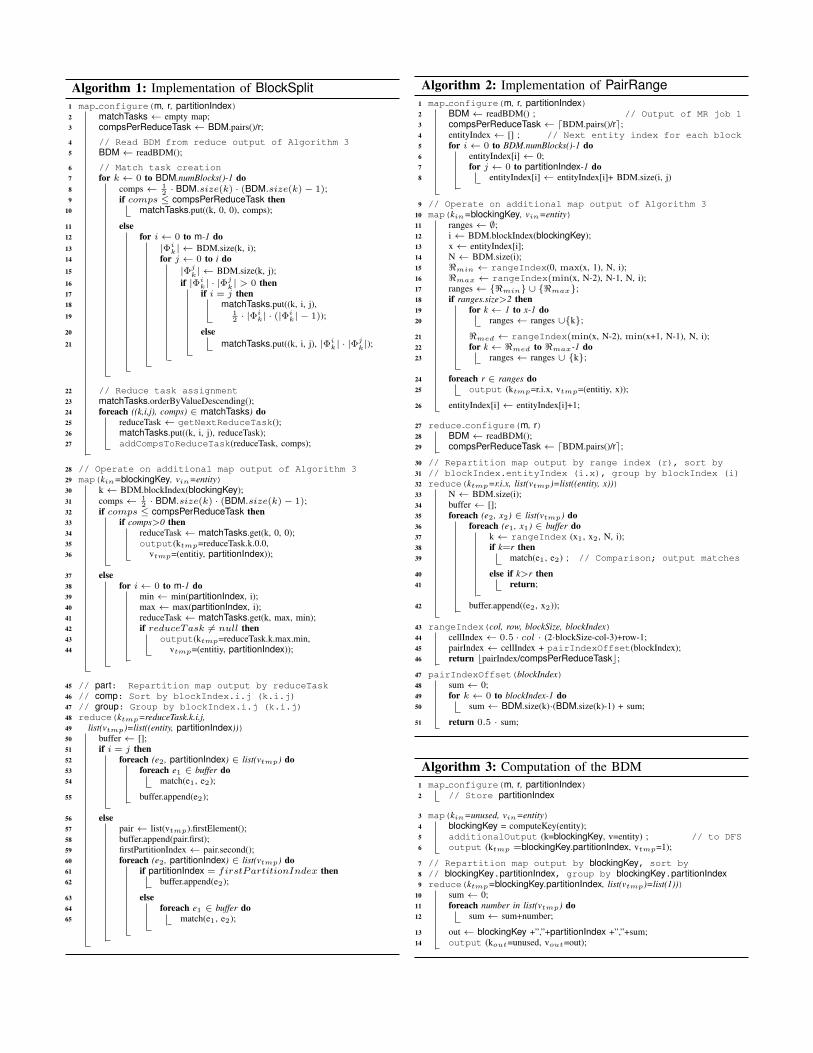
Algorithm 1: Implementation of BlockSplit1 map configure(m, r, partitionIndex)2 matchTasks ← empty map;3 compsPerReduceTask ← BDM.pairs()/r;

4 // Read BDM from reduce output of Algorithm 35 BDM ← readBDM();

6 // Match task creation7 for k ← 0 to BDM.numBlocks()-1 do8 comps ← 1

2 · BDM.size(k) · (BDM.size(k)− 1);9 if comps ≤ compsPerReduceTask then

10 matchTasks.put((k, 0, 0), comps);

11 else12 for i← 0 to m-1 do13 |Φi

k| ← BDM.size(k, i);14 for j ← 0 to i do15 |Φj

k| ← BDM.size(k, j);16 if |Φi

k| · |Φjk| > 0 then

17 if i = j then18 matchTasks.put((k, i, j),19 1

2 · |Φik| · (|Φ

ik| − 1));

20 else21 matchTasks.put((k, i, j), |Φi

k| · |Φjk|);

22 // Reduce task assignment23 matchTasks.orderByValueDescending();24 foreach ((k,i,j), comps) ∈ matchTasks) do25 reduceTask ← getNextReduceTask();26 matchTasks.put((k, i, j), reduceTask);27 addCompsToReduceTask(reduceTask, comps);

28 // Operate on additional map output of Algorithm 329 map(kin=blockingKey, vin=entity)30 k ← BDM.blockIndex(blockingKey);31 comps ← 1

2 · BDM.size(k) · (BDM.size(k)− 1);32 if comps ≤ compsPerReduceTask then33 if comps>0 then34 reduceTask ← matchTasks.get(k, 0, 0);35 output(ktmp=reduceTask.k.0.0,36 vtmp=(entitiy, partitionIndex));

37 else38 for i← 0 to m-1 do39 min ← min(partitionIndex, i);40 max ← max(partitionIndex, i);41 reduceTask ← matchTasks.get(k, max, min);42 if reduceTask 6= null then43 output(ktmp=reduceTask.k.max.min,44 vtmp=(entitiy, partitionIndex));

45 // part: Repartition map output by reduceTask46 // comp: Sort by blockIndex.i.j (k.i.j)47 // group: Group by blockIndex.i.j (k.i.j)48 reduce(ktmp=reduceTask.k.i.j,49 list(vtmp)=list((entity, partitionIndex)))50 buffer ← [];51 if i = j then52 foreach (e2, partitionIndex) ∈ list(vtmp) do53 foreach e1 ∈ buffer do54 match(e1, e2);

55 buffer.append(e2);

56 else57 pair ← list(vtmp).firstElement();58 buffer.append(pair.first);59 firstPartitionIndex ← pair.second();60 foreach (e2, partitionIndex) ∈ list(vtmp) do61 if partitionIndex = firstPartitionIndex then62 buffer.append(e2);

63 else64 foreach e1 ∈ buffer do65 match(e1, e2);

Algorithm 2: Implementation of PairRange1 map configure(m, r, partitionIndex)2 BDM ← readBDM() ; // Output of MR job 13 compsPerReduceTask ← dBDM.pairs()/re;4 entityIndex ← [] ; // Next entity index for each block5 for i← 0 to BDM.numBlocks()-1 do6 entityIndex[i] ← 0;7 for j ← 0 to partitionIndex-1 do8 entityIndex[i] ← entityIndex[i]+ BDM.size(i, j)

9 // Operate on additional map output of Algorithm 310 map(kin=blockingKey, vin=entity)11 ranges ← ∅;12 i ← BDM.blockIndex(blockingKey);13 x ← entityIndex[i];14 N ← BDM.size(i);15 <min ← rangeIndex(0, max(x, 1), N, i);16 <max ← rangeIndex(min(x, N-2), N-1, N, i);17 ranges ← {<min} ∪ {<max};18 if ranges.size>2 then19 for k ← 1 to x-1 do20 ranges ← ranges ∪{k};

21 <med ← rangeIndex(min(x, N-2), min(x+1, N-1), N, i);22 for k ← <med to <max-1 do23 ranges ← ranges ∪ {k};

24 foreach r ∈ ranges do25 output (ktmp=r.i.x, vtmp=(entitiy, x));

26 entityIndex[i] ← entityIndex[i]+1;

27 reduce configure(m, r)28 BDM ← readBDM();29 compsPerReduceTask ← dBDM.pairs()/re;

30 // Repartition map output by range index (r), sort by31 // blockIndex.entityIndex (i.x), group by blockIndex (i)32 reduce(ktmp=r.i.x, list(vtmp)=list((entity, x)))33 N ← BDM.size(i);34 buffer ← [];35 foreach (e2, x2) ∈ list(vtmp) do36 foreach (e1, x1) ∈ buffer do37 k ← rangeIndex (x1, x2, N, i);38 if k=r then39 match(e1, e2) ; // Comparison; output matches

40 else if k>r then41 return;

42 buffer.append((e2, x2));

43 rangeIndex(col, row, blockSize, blockIndex)44 cellIndex ← 0.5 · col · (2·blockSize-col-3)+row-1;45 pairIndex ← cellIndex + pairIndexOffset(blockIndex);46 return bpairIndex/compsPerReduceTaskc;

47 pairIndexOffset(blockIndex)48 sum ← 0;49 for k ← 0 to blockIndex-1 do50 sum ← BDM.size(k)·(BDM.size(k)-1) + sum;

51 return 0.5 · sum;

Algorithm 3: Computation of the BDM1 map configure(m, r, partitionIndex)2 // Store partitionIndex

3 map(kin=unused, vin=entity)4 blockingKey = computeKey(entity);5 additionalOutput (k=blockingKey, v=entity) ; // to DFS6 output (ktmp =blockingKey.partitionIndex, vtmp=1);

7 // Repartition map output by blockingKey, sort by8 // blockingKey.partitionIndex, group by blockingKey.partitionIndex9 reduce(ktmp=blockingKey.partitionIndex, list(vtmp)=list(1)))

10 sum ← 0;11 foreach number in list(vtmp) do12 sum ← sum+number;

13 out ← blockingKey +”,”+partitionIndex +”,”+sum;14 output (kout=unused, vout=out);