Quantum Position Verificationin the Random Oracle Model

Dominique Unruh

University of Tartu, Tartu, Estonia

Abstract. We present a quantum position verification scheme in the randomoracle model. In contrast to prior work, our scheme does not require boundedstorage/retrieval/entanglement assumptions. We also give an efficient position-based authentication protocol. This enables secret and authenticated commu-nication with an entity that is only identified by its position in space.

1 Introduction

What Is Position Verification? Consider the following setting: A device Pwishes to access a location-based service. This service should only be available todevices in a certain spacial region P, e.g., within a sports stadium. The serviceprovider wants to be sure no malicious device outside P accesses the service. Inother words, we need a protocol such that a prover P can prove to a verifier Vthat P is at certain location. Such a protocol is called a position verification (PV)scheme. A special case of position verification is distance bounding: P proves thathe is within a distance δ of V . In its simplest form, this is done by V sendinga random message r to P , and P has to send it back immediately. If r comesback to V in time t, P must be within distance tc/2 where c is the speed of light.In general, however, it may not be practical to require a device V in the middleof a spherical region P. (E.g., P might be a rectangular room.) In general PV,thus, we assume several verifier devices V1, . . . , Vn, and a prover P somewherein the convex hull of V1, . . . , Vn. The verifiers should then interact with P insuch a way that based on the response times of P , they can make sure that Pis at the claimed location (a kind of triangulation). Unfortunately, [5] showedthat position verification based on classical cryptography cannot be secure, evenwhen using computational assumptions, if the prover has several devices at dif-ferent locations (collusion). [4] showed impossibility in the quantum setting, butonly for information-theoretically secure protocols. Whether a protocol in thecomputational setting exists was left open.1 In this work, we close this gap andgive a simple protocol in the random oracle model.

Applications. The simplest application of PV is just for a device to provethat it is at a particular location to access a service. In a more advanced set-ting, location can be used for authentication: a prover can send a messagewhich is guaranteed to have originated within a particular region (position-based1 But both [5,4] give positive results assuming bounded retrieval/entanglement, see

“related work” below.

J.A. Garay and R. Gennaro (Eds.): CRYPTO 2014, Part II, LNCS 8617, pp. 1–18, 2014.c© International Association for Cryptologic Research 2014

2 D. Unruh

time

V1 P∗2

V2

V 1’s

msg

V2 ’s

msg

P∗1

P∗3

Fig. 1. Message flow in [4,11]. Se-curity is only guaranteed if no en-tanglement is created before theshaded region. The scheme can beattacked if P ∗

2 sends EPR pairs toP ∗1 , P

∗3 who then can execute the at-

tack from [8, Section 1].

authentication, PBA). Finally, when com-bining PBA with quantum key distribution(QKD), an encrypted message can be sentin such a way that only a recipient at acertain location can decrypt it. (E.g., thinkof sending a message to an embassy – youcan make sure that it will be received onlyin the embassy, even if you do not knowthe embassy’s public key.) More applica-tions are position-based multi-party compu-tation and position-based PKIs, see [5].

Our Contribution. We present the firstPV and PBA schemes secure against col-luding provers that do not need boundedstorage/retrieval/entanglement assump-tions. (Cf. “related work” below.) Ourprotocols use quantum cryptography and are proven secure in the (quantum)random oracle model, and they work in the 3D setting. (Actually, in any numberof dimensions, as well as in curved spacetime.2) Using [4], this also immediatelyimplies position-based QKD. (And we even get everlasting security, i.e., if theadversary breaks the hash function after the protocol run, he cannot break thesecrecy of the protocol.)

We also introduce a methodology for analyzing quantum circuits in spacetimewhich we believe simplifies the rigorous analysis of protocols that are based onthe speed of light (such as, e.g., PV or relativistic commitments [7,6]). And forthe first time (to our knowledge), a security analysis uses adaptive programmingof the quantum random oracle (in our PBA security proof).3

Related Work. [5] showed a general impossibility of computationally secure PVin the classical setting; [4] showed the impossibility of information-theoreticallysecure PV in the quantum setting. [5] proposed computationally secure protocolsfor PV and position-based key exchange in the bounded retrieval model. Theirmodel assumes that a party can only retrieve part of a large message reachingit. In particular, a party cannot forward a message (“reflection attacks” in thelanguage of [5]); this may be difficult to ensure in practice because a mirrormight be such a forwarding device. [4,11] provide a quantum protocol that issecure if the adversary can have no/limited entanglement before receiving theverifiers’ messages. (I.e., in the message flow diagram Figure 1, only in the shadedareas.) In particular, using the message flow drawn in Figure 1, the attack from

2 At the first glance, taking curvature of spacetime into account might seem likeoverkill. But for example GPS needs to take general relativity into account to ensureprecise positioning (see, e.g., [1]). There is no reason to assume that this would notbe the case for long-distance PV.

3 The semi-constant distribution technique from [13] programs the random oracle be-fore the first adversary invocation, i.e., only non-adaptive programming is possible.

Quantum Position Verification in the Random Oracle Model 3

time

t = 0

t = 1

t = 2

V1 P ∗1 P P ∗

2 V2

|Ψ〉, x1

state

ofP

∗ 1

y1

x2

state

ofP

∗ 2y 2

B := H(x1 ⊕ x2)y := measure |Ψ〉

in basis B

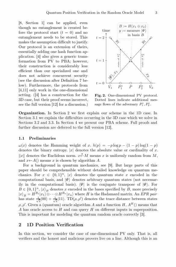
Fig. 2. One-dimensional PV protocol.Dotted lines indicate additional mes-sage flows of the adversary P ∗

1 , P∗2 .

[8, Section 1] can be applied, eventhough no entanglement is created be-fore the protocol start (t = 0) and noentanglement needs to be stored. Thismakes the assumption difficult to justify.Our protocol is an extension of theirs,essentially adding one hash function ap-plication. [4] also gives a generic trans-formation from PV to PBA; however,their construction is considerably lessefficient than our specialized one anddoes not achieve concurrent security(see the discussion after Definition 7 be-low). Furthermore, the protocols from[4,11] only work in the one-dimensionalsetting. ([4] has a construction for the3D case, but their proof seems incorrect,see the full version [12] for a discussion.)

Organization. In Section 2 we first explain our scheme in the 1D case. InSection 3.1 we explain the difficulties occurring in the 3D case which we solve inSections 3.2 and 3.3. In Section 4 we present our PBA scheme. Full proofs andfurther discussion are deferred to the full version [12].

1.1 Preliminaries

ω(x) denotes the Hamming weight of x. h(p) = −p log p − (1 − p) log(1 − p)denotes the binary entropy. |x| denotes the absolute value or cardinality of x.‖x‖ denotes the Euclidean norm. x $←M means x is uniformly random from M ,and x←A() means x is chosen by algorithm A.

For a background in quantum mechanics, see [9]. But large parts of thispaper should be comprehensible without detailed knowledge on quantum me-chanics. For x ∈ {0, 1}n, |x〉 denotes the quantum state x encoded in thecomputational basis, and |Ψ〉 denotes arbitrary quantum states (not necessar-ily in the computational basis). 〈Ψ | is the conjugate transpose of |Ψ〉. ForB ∈ {0, 1}n, |x〉B denotes x encoded in the bases specified by B, more precisely|x〉B = HB1 |x1〉⊗· · ·⊗HBn |xn〉 where H is the Hadamard matrix. An EPR pairhas state 1√

2|00〉+ 1√

2|11〉. TD(ρ, ρ′) denotes the trace distance between states

ρ, ρ′. Given a (quantum) oracle algorithm A and a function H , AH() means thatA has oracle access to H and can query H on different inputs in superposition.This is important for modeling the quantum random oracle correctly [3].

2 1D Position Verification

In this section, we consider the case of one-dimensional PV only. That is, allverifiers and the honest and malicious provers live on a line. Although this is an

4 D. Unruh

unrealistic setting, it allows us to introduce our construction and proof techniquein a simpler setting without having to consider the additional subtleties arisingfrom the geometry of intersecting light cones. We also suggest the content of thissection for teaching.

We assume the following specific setting: There are two verifiers V1 and V2

at positions −1 and 1, and an honest prover P at position 0. The verifierswill send messages at time t = 0 to the prover P , who receives them at timet = 1 (i.e., we assume units in which the speed of light is c = 1), and hisimmediate response reaches the verifiers at time t = 2. In an attack, we assumethat the malicious prover has devices P ∗

1 and P ∗2 left and right of position 0, but

no device at position 0 where the honest prover is located. See Figure 2 for adepiction of all message flows in this setting. This setting simplifies notation andis sufficient to show all techniques needed in the 1D case. The general 1D case (Pnot exactly in the middle, more malicious provers, not requiring P ’s responsesto be instantaneous) will be a special case of the higher dimensional theoremsin Section 3.3.

In this setting, we use the following PV scheme:

Definition 1 (1D position verification). Let n (number of qubits) and � (bitlength of classical challenges) be integers, 0 ≤ γ < 1/2 (fraction of allowederrors). Let H : {0, 1}� → {0, 1}n be a hash function (modeled as a quantumrandom oracle).– Before time t = 0, verifier V1 picks uniform x1, x2 ∈ {0, 1}�, y ∈ {0, 1}n and

forwards x2 to V2 over a secure channel.– At time t = 0, V1 sends |Ψ〉 and x1 to P . Here B := H(x1⊕x2), |Ψ〉 := |y〉B.

And V2 sends x2 to P .– At time t = 1, P receives |Ψ〉, x1, x2, computes B := H(x1 ⊕ x2), measures

|Ψ〉 in basis B to obtain outcome y1, and sends y1 to V1 and y2 := y1 to V2.(We assume all these actions are instantaneous, so P sends y1, y2 at timet = 1.)

– At time t = 2, V1 and V2 receive y1, y2. Using secure channels, they checkwhether y1 = y2 and ω(y1 − y) ≤ γn. If so (and y1, y2 arrived in time), theyaccept.

We can now prove security in our simplified setting.

Theorem 2 (1D position verification). Assume P ∗1 and P ∗

2 perform at mostq queries to H. Then in an execution of V1, V2, P

∗1 , P

∗2 with V1, V2 following the

protocol from Definition 1, the probability that V1, V2 accept is at most 4

2q2−�/2 +(2h(γ)

1 +√1/2

2

)n

.

Proof. To prove this theorem, we proceed using a sequence of games. The firstgame is the original protocol execution, and in the last game, we will be ableto show that Pr[Accept] is small. Here we abbreviate the event “y1 = y2 andω(y1 − y) ≤ γn” as “Accept”.4 This probability is negligible if γ ≤ 0.037 and n, � are superlogarithmic.

Quantum Position Verification in the Random Oracle Model 5

time

t = 0

t = 1

t = 2

V1 V2

|Ψ〉, x1

y 2

x2

y1 ba

rrie

r

pick Bprogram H

no proverhere

AH1

AH2

x1 known here

x2 known here

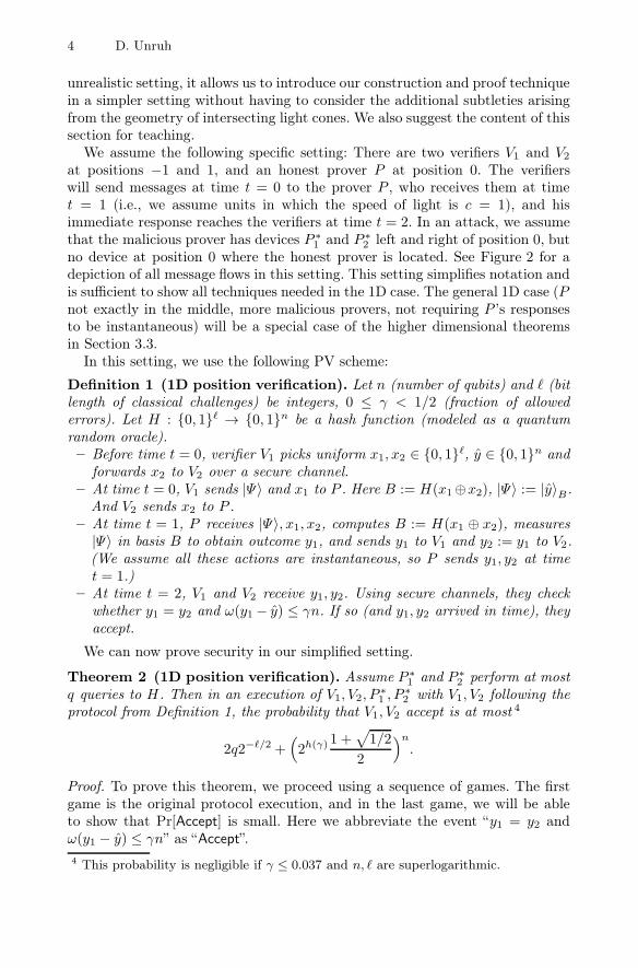
Fig. 3. Spacetime diagram depicting various stepsof the proof of Theorem 2

Game 1. An execution as de-scribed in Theorem 2.

As a first step, we use EPRpairs to delay the choice ofthe basis B. This is a stan-dard trick that has been usedin QKD proofs and other set-tings. By choosing B suffi-ciently late, we will be able toargue below that B is indepen-dent of the state of P ∗

1 and P ∗2 .

Game 2. As in Game 1, ex-cept that V1 prepares n EPRpairs, with their first qubits inregister X and their secondqubits in Y . Then V1 sends Xat time t = 0 instead of send-ing |Ψ〉. At time t = 2, V1 measures Y in basis B := H(x1 ⊕ x2), the outcomeis y.

Note in particular that V1, V2 never query H before time t = 2. (But P ∗1 , P

∗2

might, of course.) It is easy to verify (and well-known) that for any B ∈ {0, 1},preparing a qubit X := |y〉B for random y ∈ {0, 1} is perfectly indistinguishable(when given X, y,B) from producing an EPR pair XY , and then measuring Yin bases B to get outcome y. Thus Pr[Accept : Game 1] = Pr[Accept : Game 2].

The problem now is that, although we have delayed the time when the basisB is used, the basis is still chosen early: At time t = 0, the values x1, x2 arechosen, and those determine B via B = H(x1 ⊕ x2). We have that neither P ∗

1

nor P ∗2 individually knows B, but that does not necessarily exclude an attack.

(For example, [8, Section 1] gives an efficient attack for the case that H is theidentity, even though in this case B would still not be known to P ∗

1 nor P ∗2

individually before time t = 1.) We can only hope that H is a sufficiently complexfunction such that computationally, B is “as good as unknown” before time t = 1(where x1 and x2 become known to both P ∗

1 , P ∗2 ). The next game transformation

formalizes this:

Game 3. As in Game 1, except that at time t = 1, the value B$←{0, 1}n is

chosen, and the random oracle is reprogrammed to return H(x1 ⊕ x2) = B aftert = 1.

To clarify this, if H0 : {0, 1}� → {0, 1}n denotes a random function chosenat the very beginning of the execution, then at time t ≤ 1, H(x) = H0(x) forall x ∈ {0, 1}�, while at time t > 1, H(x0 ⊕ x1) = B and H(x) = H0(x) for allx �= x0 ⊕ x1.

Intuitively, the change between Games 2 and 3 cannot be noticed becausebefore time t = 1, the verifiers never query H(x1 ⊕ x2), and the provers cannot

6 D. Unruh

query H(x1⊕x2) either: before time t, in no spacial location the prover will haveaccess to both x1 and x2.

This is illustrated in Figure 3: The hatched areas represent where x1 and x2

are known respectively. Note that they do not overlap. The dashed horizontalline represents where the random oracle is programmed (t = 1).

Purists may object that choosing B and programming the random oracle toreturn B at all locations in a single instant in time needs superluminal com-munication which in turn is know to violate causality and might thus lead toinconsistent reasoning. Readers worried about this aspect should wait until weprove the general case of the PV protocol in Section 3.3, there this issue willnot arise because we first transform the whole protocol execution into a non-relativistic quantum circuit and perform the programming of the random oraclein that circuit.

To prove that Games 2 and 3 are indistinguishable, we use the followinglemma shown in the full version.

Lemma 3. Let H : {0, 1}� → {0, 1}n be a random oracle. Let (A1, A2) be oraclealgorithms sharing state between invocations that perform at most q queries toH. Let C1 be an oracle algorithm that on input (j, x) does the following: RunAH

1 (x) till the j-th query to H, then measure the argument of that query in thecomputational basis, and output the measurement outcome. (Or ⊥ if no j-thquery occurs.) Let

P 1A := Pr[b′ = 1 : H

$←({0, 1}� → {0, 1}n), x←{0, 1}�, AH1 (x), b′←AH

2 (x,H(x))]

P 2A := Pr[b′ = 1 : H

$←({0, 1}� → {0, 1}n), x←{0, 1}�, B $←{0, 1}n,AH

1 (x),H(x) := B, b′←AH2 (x,B)]

PC := Pr[x = x′ : H $←({0, 1}� → {0, 1}n), x←{0, 1}�, j $←{1, . . . , q}, x′←CH1 (j, x)]

Then |P 1A − P 2

A| ≤ 2q√PC .

In other words, an adversary can only notice that the random oracle is repro-grammed at position x if he can guess x before the reprogramming takes place.

To apply Lemma 3 to Games 2 and 3, let AH1 (x) be the machine that executes

verifiers and provers from Game 2 until time t = 1 (inclusive). When V1 choosesx1, x2, AH

1 (x) chooses x1$←{0, 1}� and x2 := x ⊕ x1. And let AH

2 (x,B) be themachine that executes verifiers and provers after time t = 1. When V1 queriesH(x1 ⊕ x2), AH

2 uses the value B instead. In the end, AH2 returns 1 iff y1 = y2

and ω(y − y1) ≤ γn. (See Figure 3 for the time intervals handled by AH1 ,AH

2 .)Since V1, V2 make no oracle queries except for H(x1⊕x2), and since P ∗

1 , P∗2 make

at most q oracle queries, we have that AH1 , AH

2 perform at most q queries.By construction, P 1

A = Pr[Accept : Game 2]. And P 2A = Pr[Accept : Game 3].

And PC = Pr[x′ = x1 ⊕ x2 : Game 4] for the following game:

Game 4. Pick j$←{1, . . . , q}. Then execute Game 2 till time t = 1 (inclusive),

but stop at the j-th query and measure the query register. Call the outcome x′.

Quantum Position Verification in the Random Oracle Model 7

Since Game 4 executes only till time t = 1, and since till time t = 1, no gate canbe reached by both x1, x2 (note: at time t = 1, at position 0 both x1, x2 could beknown, but no malicious prover may be at that location), the probability thatx1⊕x2 will be guessed is bounded by 2−�. Hence Pr[x′ = x1⊕x2 : Game 3] ≤ 2−�.(This argument was a bit nonrigorous; we will be more precise in the proof ofthe generic case, in the proof of Theorem 6.)

Thus by Lemma 3, we have∣∣Pr[Accept : Game 2]− Pr[Accept : Game 3]

∣∣ = |P 1A − P 2

A| ≤ 2q√PC

= 2q√Pr[x′ = x1 ⊕ x2 : Game 4] ≤ 2q2−�/2. (1)

We continue to modify Game 3.

Game 5. Like Game 3, except that for time t > 1, we install a barrier at po-sition 0 (i.e., where the honest prover P would be) that lets no informationthrough.

The barrier is illustrated in Figure 3 with a thick vertical line.Time t = 1 is latest time at which information from position 0 could reach

the verifiers V1, V2 at time t ≤ 2. Since we install the barrier only for timet > 1, whether the barrier is there or not cannot influence the measurements ofV1, V2 at time t = 2. And Accept only depends on these measurements. ThusPr[Accept : Game 3] = Pr[Accept : Game 5].

Let ρ be the state of the execution of Game 5 directly after time t = 1 (i.e.,after the gates at times t ≤ 1 have been executed). Then ρ is a threepartitestate consisting of registers Y , L, R where Y is the register containing the EPRqubits which will be measured to give y (cf. Game 2), and L and R are thequantum state left and right of the barrier respectively. Then y is the resultof measuring Y in basis B, and y1 is the result of applying some measurementM1 to L (consisting of all the gates left of the barrier), and y2 is the result ofapplying some measurement M2 to R. Notice that due to the barrier, M1 andM2 operate only on L and R, respectively, without interaction between thosetwo. We have thus:

Pr[Accept : Game 5] = Pr[y1 = y2 and ω(y − y1) ≤ γn : B$←{0, 1}n, Y LR←ρ,

y←MB(Y ), y1←M1(L), y2←M2(R)]

where Y LR←ρ means initializing Y LR with state ρ. And MB is a measurementin bases B. And y←MB(Y ) means measuring register Y using measurementMB and assigning the result to y. And y1←M1(L), y2←M2(R) analogously.

The rhs of this equation is a so-called monogamy of entanglement game,

and [11] shows that the rhs is bounded by(2h(γ)

1+√

1/2

2

)n

. Thus Pr[Accept :

Game 5] ≤(2h(γ)

1+√

1/2

2

)n

. And from (1) and the equalities between games,

we have∣∣Pr[Accept : Game 1]− Pr[Accept : Game 5]

∣∣ ≤ 2q2−�/2.

Thus altogether Pr[Accept : Game 1] ≤ 2q2−�/2 +(2h(γ)

1+√

1/2

2

)n

. �

8 D. Unruh

R1

R2 R3

|Ψ〉x1

x2 x3P

V1

V2 V3

R1

R2 R3tδ ≈

1.13√ 32

≈0.86 δ

V1

V2 V3

(a) (b)

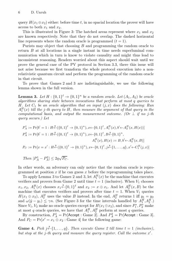
Fig. 4. The geometry of space at time tδ (i.e., when B first becomes known). Left forδ = 0, right for δ =

√4−√

12− 12≈ 0.23.

3 Position Verification in Higher Dimensions

3.1 Difficulties

Excepting special cases where the honest prover happens to lie on a line betweentwo verifiers, one-dimensional PV with two verifiers is not very useful. We there-fore need to generalize the approach to three dimensions. It turns out that somenon-trivialities occur here. For n-dimensional PV we need at least n+1 verifiers.5To illustrate the problems occurring in the higher dimensional case, we sketchwhat happens if we try to generalize the protocol and proof from Section 2 tothe 2D case.

In the 2D case we need at least three verifiers V1, V2, V3. Let’s assume thatthey are arranged in a equilateral triangle, each at distance 1 from an honestprover P in the center. (Cf. Figure 4 (a).) V1 sends a quantum state |Ψ〉, andall Vi send a random xi. At time t = 1, all xi are received by P who computesB := H(x1 ⊕ x2 ⊕ x3) and measures |Ψ〉 in basis B, yielding the value y to besent to V1, V2, V3.

Now as in Section 2 we can argue that before time t = 1, there is no point inspace where all x1, x2, x3 are known. Hence B := H(x1 ⊕ x2 ⊕ x3) will not bequeried before t = 1. Hence by programming the random oracle (using Lemma 3)we can assume that the basis B is chosen randomly only at time t = 1. InSection 2 we then observed that space is partitioned into two disjoint regions:5 PV (in Euclidean space) can only work if the prover P is in the convex hull C of the

verifiers. Otherwise, if we project P onto the hypersurface H separating C from P ,we get a point P ′ that is closer to any point of C than P . Since the convex hull of nprovers can at most be n− 1 dimensional, we need at least n+ 1 provers to get ann dimensional convex hull.

Quantum Position Verification in the Random Oracle Model 9

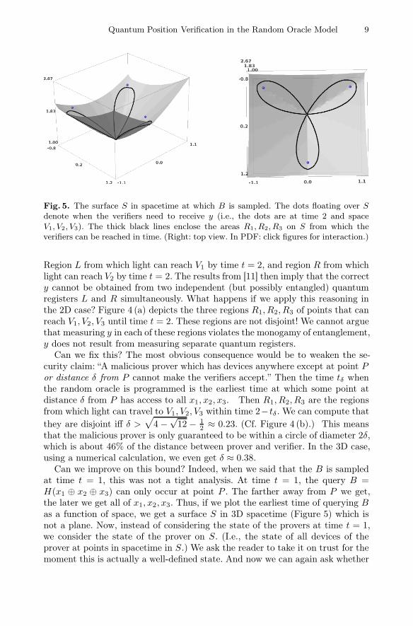
Fig. 5. The surface S in spacetime at which B is sampled. The dots floating over Sdenote when the verifiers need to receive y (i.e., the dots are at time 2 and spaceV1, V2, V3). The thick black lines enclose the areas R1, R2, R3 on S from which theverifiers can be reached in time. (Right: top view. In PDF: click figures for interaction.)

Region L from which light can reach V1 by time t = 2, and region R from whichlight can reach V2 by time t = 2. The results from [11] then imply that the correcty cannot be obtained from two independent (but possibly entangled) quantumregisters L and R simultaneously. What happens if we apply this reasoning inthe 2D case? Figure 4 (a) depicts the three regions R1, R2, R3 of points that canreach V1, V2, V3 until time t = 2. These regions are not disjoint! We cannot arguethat measuring y in each of these regions violates the monogamy of entanglement,y does not result from measuring separate quantum registers.

Can we fix this? The most obvious consequence would be to weaken the se-curity claim: “A malicious prover which has devices anywhere except at point Por distance δ from P cannot make the verifiers accept.” Then the time tδ whenthe random oracle is programmed is the earliest time at which some point atdistance δ from P has access to all x1, x2, x3. Then R1, R2, R3 are the regionsfrom which light can travel to V1, V2, V3 within time 2− tδ. We can compute thatthey are disjoint iff δ >

√4−√

12 − 12 ≈ 0.23. (Cf. Figure 4 (b).) This means

that the malicious prover is only guaranteed to be within a circle of diameter 2δ,which is about 46% of the distance between prover and verifier. In the 3D case,using a numerical calculation, we even get δ ≈ 0.38.

Can we improve on this bound? Indeed, when we said that the B is sampledat time t = 1, this was not a tight analysis. At time t = 1, the query B =H(x1 ⊕ x2 ⊕ x3) can only occur at point P . The farther away from P we get,the later we get all of x1, x2, x3. Thus, if we plot the earliest time of querying Bas a function of space, we get a surface S in 3D spacetime (Figure 5) which isnot a plane. Now, instead of considering the state of the provers at time t = 1,we consider the state of the prover on S. (I.e., the state of all devices of theprover at points in spacetime in S.) We ask the reader to take it on trust for themoment this is actually a well-defined state. And now we can again ask whether

10 D. Unruh

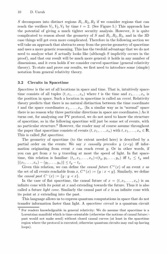
S decomposes into distinct regions R1, R2, R3 if we consider regions that canreach the verifiers V1, V2, V3 by time t = 2. (See Figure 5.) This approach hasthe potential of giving a much tighter security analysis. However, it is quitecomplicated to reason about the geometry of S and R1, R2, R3, and in the 3Dcase things will get even more complicated. Therefore in the following section wewill take an approach that abstracts away from the precise geometry of spacetimeand uses a more generic reasoning. This has the twofold advantage that we do notneed to analyze what S actually looks like (although S implicitly occurs in theproof), and that our result will be much more general: it holds in any number ofdimensions, and it even holds if we consider curved spacetime (general relativitytheory). To state and prove our results, we first need to introduce some (simple)notation from general relativity theory.

3.2 Circuits in Spacetime

Spacetime is the set of all locations in space and time. That is, intuitively space-time consists of all tuples (t, x1, . . . , xn) where t is the time and x1, . . . , xn isthe position in space. Such a location in spacetime is called an event. Relativitytheory predicts that there is no natural distinction between the time coordinatet and the space coordinates x1, . . . , xn. (In a similar way as in “normal” spacethere is no reason why three particular directions in space are coordinates.) As itturns out, for analyzing our PV protocol, we do not need to know the structureof spacetime, so in the following spacetime will just be some set of events, withno particular structure.6 However, the reader may of course assume throughoutthe paper that spacetime consists of events (t, x1, . . . , xn) with t, x1, . . . , xn ∈ �.This is called flat spacetime.

The geometry of spacetime (to the extent needed here) is described by apartial order on the events: We say x causally precedes y (x≺y) iff infor-mation originating from event x can reach event y. Or in other words, ifyou can get from x to y traveling at most the speed of light. In flat space-time, this relation is familiar: (tx, x1, . . . , xn)≺(ty, y1, . . . , yn) iff tx ≤ ty and‖(x1, . . . , xn)− (y1, . . . , yn)‖ ≤ ty − tx.

Given this relation, we can define the causal future C+(x) of an event x asthe set of all events reachable from x, C+(x) := {y : x ≺ y}. Similarly, we definethe causal past C−(x) := {y : y ≺ x}.

In the case of flat spacetime, the causal future of x = (t, x1, . . . , xn) is aninfinite cone with its point at x and extending towards the future. Thus it is alsocalled a future light cone. Similarly the causal past of x is an infinite cone withits point at x extending into the past.

This language allows us to express quantum computations in space that do nottransfer information faster than light. A spacetime circuit is a quantum circuit6 For readers knowledgeable in general relativity: We do assume that spacetime is a

Lorentzian manifold which is time-orientable (otherwise the notions of causal future/-past would not make send) without closed causal curves (at least in the spacetimeregion where the protocol is executed; otherwise quantum circuits may end up havingloops).

Quantum Position Verification in the Random Oracle Model 11

where every gate is at a particular event. There can only be a wire from a gate atevent x to a gate at event y if x causally precedes y (x ≺ y). Note that since ≺ is apartial order and thus antisymmetric, this ensures that a circuit cannot be cyclic.Note further that there is no limit to how much computation can be performedin an instant since ≺ is reflexive. We can model malicious provers that are notat the location of an honest prover by considering circuits with no gates in P,where P is a region in spacetime. (This allows for more finegrained specificationsthan, e.g., just saying that the malicious prover is not within δ distance of thehonest prover. For example, P might only consist of events within a certaintime interval; this means that the malicious prover is allowed to be at any spacelocation outside that time interval.) Notice that a spacetime circuit is also just anormal quantum circuit if we forget where in spacetime gates are located. Thustransformations on quantum circuits (such as changing the execution order ofcommuting gates) can also be applied to spacetime circuits, the result will be avalid circuit, though possibly not a spacetime circuit any more.

3.3 Achieving Higher-Dimensional Position Verification

We can now formulate the definition of secure PV in higher dimensions usingthe language from the previous section.

Definition 4 (Sound position verification). Let P be a region in spacetime.A position verification protocol is sound for P iff for any non-uniform polynomial-time7 spacetime circuit P ∗ that has no gates in P, the following holds: In aninteraction between the verifiers and P ∗, the probability that the verifiers accept(the soundness error) is negligible.

The smaller the region P is, the better the protocol localizes the prover. Infor-mally, we say the protocol has higher precision if P is smaller.

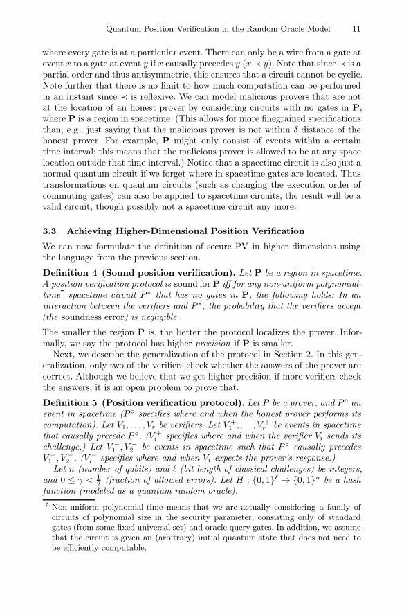
Next, we describe the generalization of the protocol in Section 2. In this gen-eralization, only two of the verifiers check whether the answers of the prover arecorrect. Although we believe that we get higher precision if more verifiers checkthe answers, it is an open problem to prove that.

Definition 5 (Position verification protocol). Let P be a prover, and P ◦ anevent in spacetime (P ◦ specifies where and when the honest prover performs itscomputation). Let V1, . . . , Vr be verifiers. Let V +

1 , . . . , V +r be events in spacetime

that causally precede P ◦. (V +i specifies where and when the verifier Vi sends its

challenge.) Let V −1 , V −

2 be events in spacetime such that P ◦ causally precedesV −1 , V −

2 . (V −i specifies where and when Vi expects the prover’s response.)

Let n (number of qubits) and � (bit length of classical challenges) be integers,and 0 ≤ γ < 1

2 (fraction of allowed errors). Let H : {0, 1}� → {0, 1}n be a hashfunction (modeled as a quantum random oracle).7 Non-uniform polynomial-time means that we are actually considering a family of

circuits of polynomial size in the security parameter, consisting only of standardgates (from some fixed universal set) and oracle query gates. In addition, we assumethat the circuit is given an (arbitrary) initial quantum state that does not need tobe efficiently computable.

12 D. Unruh

– The verifiers choose uniform x1, . . . , xr ∈ {0, 1}�, y ∈ {0, 1}n. (By commu-nicating over secure channels.)

– At some event that causally precedes P ◦, V0 sends |Ψ〉 to P . Here B :=H(x1 ⊕ · · · ⊕ xr), |Ψ〉 := |y〉B.

– For i = 1, . . . , r: Vr sends xr to P at event V +r .

– At event P ◦, P will have |Ψ〉, x1, . . . , xr. Then P computes B := H(x1 ⊕· · · ⊕ xr), measures |Ψ〉 in basis B to obtain outcome y1, and sends y1 to V1

and y2 := y1 to V2.– At events V −

1 , V −2 , V1 and V2 receive y1, y2. Using secure channels, the ver-

ifiers check whether y1 = y2 and ω(y1 − y) ≤ γn. If so (and y1, y2 indeedarrived at V −

1 , V −2 ), the verifiers accept.

In the protocol description, for simplicity we assume that V1, V2 are the re-ceiving verifiers. However, there is no reason not to choose other two verifiers, oreven additional verifiers not used for sending. Similarly, |Ψ〉 could be sent by anyverifier, or by an additional verifier. In the analysis, we only use the events atwhich different messages are sent/received, not which verifier device sends whichmessage.

Note that this protocol also allows for realistic provers that cannot performinstantaneous computations: In this case, one chooses the events V −

1 , V −2 such

that the prover’s messages can still reach them even if the prover sends y1, y2with some delay.

We can now state the main security result:

Theorem 6. Assume that γ ≤ 0.037 and n, � are superlogarithmic.Then the PV protocol from Definition 5 is sound for P :=

⋂ri=1 C

+(V +i ) ∩

C−(V −1 ) ∩ C−(V −

2 ). (In words: There is no event in spacetime outside of P atwhich one can receive the messages xi from all Vi, and send messages that willbe received in time by V1, V2.)

Concretely, if the malicious prover performs at most q oracle queries, then the

soundness error is at most ν :=(2h(γ)

1+√

1/2

2

)n

+ 2q2−�/2.

Notice that the condition on the locations of the provers is tight: If E ∈⋂ri=1 C

+(V +i ) ∩ C−(V −

1 ) ∩ C−(V −2 ) \ P �= ∅, then the protocol could even be

broken by a malicious prover with a single device: P ∗ could be at event E, receivex1, . . . , xr, compute y1, y2 honestly, and send them to V1, V2 in time. The samereasoning applies to any protocol where only two verifiers receive. Our protocolis thus optimal in terms of precision under all such protocols.

Proof of Theorem 6. In the following, we write short C+i for C+(V +

i ) and C−i

for C−(V −i ). We also write

⋂instead of

⋂ri=1. The precondition of the theorem

then becomes:⋂C+

i ∩C−1 ∩ C−

2 ⊆ P. Let Ω denote all of spacetime.We now partition the gates in the spacetime circuit P ∗ into several disjoint

sets of gates (subcircuits), depending on where they are located in spacetime.For each subcircuit, we also give an rough intuitive meaning; those meaningsare not precisely what the subcircuits do but help to guide the intuition in theproof.

Quantum Position Verification in the Random Oracle Model 13

Subcircuit Region in spacetime IntuitionP ∗pre (C−

1 ∪C−2) \

⋂C+

i PrecomputationP ∗P

⋂C+

i ∩ C−1 ∩ C−

2 Gates in P (empty)P ∗1

⋂C+

i ∩ C−1 \ C−

2 Computing y1P ∗2

⋂C+

i ∩ C−2 \ C−

1 Computing y2P ∗post Ω \ C−

1 \ C−2 After protocol end

Note that all those subcircuits are disjoint, and their union is all of Ω. Thesubcircuits have analogues in the proof in the one-dimensional case. P ∗

pre corre-sponds to the gates below the dashed line in Figure 3; P ∗

1 to the gates abovethe dashed line and left of the barrier; P ∗

2 above the dashed line and right ofthe barrier; P ∗

post to everything that is above the picture. This correspondanceis not exact, because as discussed in Section 3.1, the dashed line needs to bereplaced by a surface S (Figure 5) which is not flat. In our present notation, Sis the border between P ∗

pre and the other subcircuits.In addition, in some abuse of notation, by V1 we denote the circuit at V −

1 thatreceives y1. Similar for V2.

By definition of spacetime circuits, there can only be a wire from gate G1 togate G2 if G1, G2 are at events E1, E2 with E1≺E2 (E1 causally precedes E2).Thus, by definition of causal futures and the transitivity of ≺, there can be nowire leaving C+

i. Similarly, there can be no wire entering C−i. These two facts

are sufficient to check the following facts:

P ∗1 , P

∗2 , P

∗post�P ∗

pre, P ∗1�P ∗

2 , P ∗2�P ∗

1 ,

P ∗1�V2, P ∗

2�V1, P ∗post�P ∗

1 , P∗2 , V1, V2.

(2)

Here A�B means that there is no wire from subcircuit A to subcircuit B.Given these subcircuits, we can write the execution of the protocol as the

following quantum circuit:

P ∗pre

P ∗1

P ∗2

V1

V2

y1

y2

x

P ∗post

|x〉B

(3)

Here x is short for x1, . . . , xr. And we have omitted wires between subcircuitsthat are in the transitive hull of the wires drawn. (E.g., there can be a wire fromP ∗pre to V1, but we did not draw it because we drew wires from P ∗

pre to P ∗1 to

V1.) Note that P ∗P does not occur in this circuit, because it contains no gates (it

consists of gates in⋂C+

i ∩ C−1 ∩ C−

2 = P which by assumption contains nogates).

From (2) it follows that no wires are missing in (3). In particular, (2) impliesthat the quantum circuit is well-defined. If we did not have, e.g., P ∗

1�P ∗pre, there

might be wires between P ∗1 and P ∗

pre in both directions; the result would not bea quantum circuit. We added arrow heads in (2), these are only to stress that thewires indeed go in the right directions, below we will follow the usual left-to-rightconvention in quantum circuits and omit the arrow heads.

14 D. Unruh

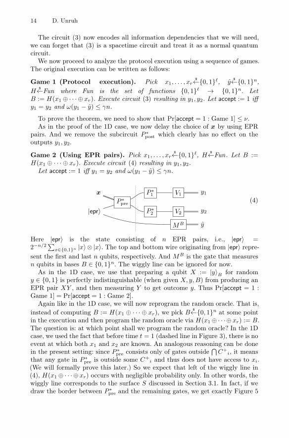
The circuit (3) now encodes all information dependencies that we will need,we can forget that (3) is a spacetime circuit and treat it as a normal quantumcircuit.

We now proceed to analyze the protocol execution using a sequence of games.The original execution can be written as follows:

Game 1 (Protocol execution). Pick x1, . . . , xr$←{0, 1}�, y

$←{0, 1}n,H

$←Fun where Fun is the set of functions {0, 1}� → {0, 1}n. LetB := H(x1 ⊕ · · · ⊕ xr). Execute circuit (3) resulting in y1, y2. Let accept := 1 iffy1 = y2 and ω(y1 − y) ≤ γn.

To prove the theorem, we need to show that Pr[accept = 1 : Game 1] ≤ ν.As in the proof of the 1D case, we now delay the choice of x by using EPR

pairs. And we remove the subcircuit P ∗post which clearly has no effect on the

outputs y1, y2.

Game 2 (Using EPR pairs). Pick x1, . . . , xr$←{0, 1}�, H

$←Fun. Let B :=H(x1 ⊕ · · · ⊕ xr). Execute circuit (4) resulting in y1, y2.

Let accept := 1 iff y1 = y2 and ω(y1 − y) ≤ γn.

P ∗pre

P ∗1

P ∗2

V1

V2

y1

y2

x

|epr〉MB y

(4)

Here |epr〉 is the state consisting of n EPR pairs, i.e., |epr〉 =2−n/2

∑x∈{0,1}n |x〉⊗ |x〉. The top and bottom wire originating from |epr〉 repre-

sent the first and last n qubits, respectively. And MB is the gate that measuresn qubits in bases B ∈ {0, 1}n. The wiggly line can be ignored for now.

As in the 1D case, we use that preparing a qubit X := |y〉B for randomy ∈ {0, 1} is perfectly indistinguishable (when given X, y,B) from producing anEPR pair XY , and then measuring Y to get outcome y. Thus Pr[accept = 1 :Game 1] = Pr[accept = 1 : Game 2].

Again like in the 1D case, we will now reprogram the random oracle. That is,instead of computing B := H(x1 ⊕ · · · ⊕ xr), we pick B

$←{0, 1}n at some pointin the execution and then program the random oracle via H(x1 ⊕ · · ·⊕xr) := B.The question is: at which point shall we program the random oracle? In the 1Dcase, we used the fact that before time t = 1 (dashed line in Figure 3), there is noevent at which both x1 and x2 are known. An analogous reasoning can be donein the present setting: since P ∗

pre consists only of gates outside⋂C+

i, it meansthat any gate in P ∗

pre is outside some C+i and thus does not have access to xi.

(We will formally prove this later.) So we expect that left of the wiggly line in(4), H(x1 ⊕ · · · ⊕ xr) occurs with negligible probability only. In other words, thewiggly line corresponds to the surface S discussed in Section 3.1. In fact, if wedraw the border between P ∗

pre and the remaining gates, we get exactly Figure 5

Quantum Position Verification in the Random Oracle Model 15

(in the 2D case at least). However, the approach of decomposing spacetime intosubcircuits removes the necessity of dealing with the exact geometry of S.

Formally, we will need to apply Lemma 3. Given a function H and valuesx,B, let Hx �→B denote the function identical to H , except that Hx �→B(x) = B.Let AH

1 (x) denote the oracle machine that picks x1, . . . , xr−1$←{0, 1}� and sets

xr := x ⊕ x1 ⊕ · · · ⊕ xr−1 and prepares the state |epr〉 and then executes P ∗pre.

Let AH2 (x,B) denote the oracle machine that, given the state from AH

1 , executesP ∗1 , P

∗2 , V1, V2,M

B with oracle access to Hx �→B instead of H , sets accept := 1 iffy1 = y2 and ω(y1 − y) ≤ γn, and returns accept. Let C1, P

1A, P

2A, PC be defined

as in Lemma 3. Then by construction, P 1A = Pr[accept = 1 : Game 2] (using the

fact that H = Hx �→H(x)). And P 2A = Pr[accept = 1 : Game 3] for the following

game:

Game 3 (Reprogramming H). Pick x1, . . . , xr$←{0, 1}�, H

$←Fun. Executecircuit (4) until the wiggly line (with oracle access to H). Pick B

$←{0, 1}n. Ex-ecute circuit (4) after the wiggly line (with oracle access to Hx �→B) resulting iny1, y2, y. Let accept := 1 iff y1 = y2 and ω(y1 − y) ≤ γn.And finally PC = Pr[x′ = x1 ⊕ · · · ⊕ xr : Game 4] for the following game:

Game 4 (Guessing x1 ⊕ · · · ⊕ xr). Pick x1, . . . , xr$←{0, 1}�, H

$←Fun, andj

$←{1, . . . , q}. Prepare |epr〉 and execute circuit P ∗pre until the j-th query to H.

Measure the argument x′ of that query.By Lemma 3, we have |P 1

A − P 2A| ≤ 2q

√PC . Thus, abbreviating x = x1⊕· · ·⊕xr

as guessX, we have∣∣Pr[accept = 1 : Game 2]− Pr[accept = 1 : Game 3]

∣∣≤ 2q

√Pr[guessX : Game 4]. (5)

We now focus on Game 3. Let ρY LR denote the state in circuit (4) at the wigglyline (for random x1, . . . , xr, H). Let L refer to the part of ρY LR that is on thewires entering P ∗

1 , and R refer to the part of ρLR on the wires entering P ∗2 . Let

Y refer to the lowest wire (containing EPR qubits). Notice that we have nowreproduced the situation from the 1D case where space is split into two separateregisters R and L, and the computation of y1, y2 is performed solely on R, L,respectively. In fact, we have now also identified the regions R1, R2 from thediscussion in Section 3.1 (Figure 5): R1 is the boundary between P ∗

pre and P ∗1 ;

analogously R2. (R3 from Figure 5 has no analogue here because V3 does notreceive here.) For given B, let ML(B) be the POVM operating on L consisting ofP ∗1 and V1. (ML can be modeled as a POVM because P ∗

1 and V1 together returnonly a classical value and thus constitute a measurement.) Let MR(B) be thePOVM operating on R consisting of P ∗

2 and V2. Then we can rewrite Game 3as:Game 5 (Monogamy game). Prepare ρY LR. Pick B

$←{0, 1}n. Apply mea-surement ML(B) to L, resulting in y1. Apply measurement MR(B) to R, result-ing in y2. Measure Y in basis B, resulting in y. Let accept := 1 iff y1 = y2 andω(y1 − y) ≤ γn.

16 D. Unruh

Then Pr[accept = 1 : Game 3] = Pr[accept = 1 : Game 5]. Furthermore, Game 5is again a monogamy of entanglement game, and [11] shows that Pr[accept =

1 : Game 5] ≤(2h(γ)

1+√

1/2

2

)n

. We can furthermore show (see the full version

[12]) that Pr[guessX : Game 4] ≤ 2−�. With (5) we get

Pr[accept = 1 : Game 1] ≤(2h(γ)

1 +√1/2

2

)n

+ 2q2−�/2 = ν.

Numerically, we can verify that for γ ≤ 0.037, we have 2h(γ)1+

√1/2

2 < 1 andthus ν is negligible (for superlogarithmic n, � and polynomially bounded q). �In Flat Spacetime. Theorem 6 tells us where in spacetime a prover can bethat passes verification. (Region P.) However, the theorem is quite general; it isnot immediate what this means in the concrete setting of flat spacetime. In thefull version [12] we derive specialized criteria for flat spacetime and show thatTheorem 6 implies that a prover can be precisely localized by verifiers arrangedas a tetrahedron.

4 Position-Based Authentication

Position verification is, in itself, a primitive of somewhat limited use. It guaran-tees that no prover outside the region P can pass the verification. Yet nothingforbids a prover to just wait until some other honest party has successfully passedposition verification, and then to impersonate that honest party. To realize theapplications described in the introduction, we need a stronger primitive thatnot only proves that a prover is at a specific location, but also allows him tobind this proof to specific data. (The difference is a bit like that between iden-tification schemes and message authentication schemes.) Such a primitive is beposition-based authentication. This guarantees that the malicious prover cannotauthenticate a message m unless he is in region P (or some honest party atlocation m wishes to authenticate that message).

Definition 7 (Secure position-based authentication). A position-basedauthentication (PBA) scheme is a PV scheme where provers and verifiers get anadditional argument m, a message to be authenticated.

Let P be a region in spacetime. A position-based authentication (PBA) protocolis sound for P iff for any non-uniform polynomial-time spacetime circuit P ∗ thathas no gates in P, the probability that the challenge verifiers ( soundness error)accept is negligible in the following execution:

P ∗ picks a message m∗ and then interacts with honest verifiers (called thechallenge verifiers) on input m∗. Before, during, and after that interaction, P ∗

may spawn instances of the honest prover and honest verifiers, running on inputsm �= m∗. These instances run concurrently with P ∗ and the challenge verifiersand P ∗ may arbitrarily interact with them. Note that the honest prover/honestverifier instances may have gates in P.

Quantum Position Verification in the Random Oracle Model 17

PBA was already studied in [4]. They give a generic transformation to con-vert a PV protocol into a PBA. The generic solution has two drawbacks, though:

– It needs Ω(�μ) invocations of the PV protocol forell-bit messages and 2−μ security level. (Our protocol below will need onlyone invocation.)

– It is only secure if a single instance of the honest prover runs concurrently. Ifthe malicious prover can suitably interleave several instances of the honestprover, he can authenticate arbitrary messages.

(We do not know whether their solution gives adaptive security, i.e., whetherthe adversary can choose m∗ and the honest provers’ inputs m depending oncommunication he has seen before.) Although we do not have a generic trans-formation from PV to PBA that solves these issues, a small modification of ourPV protocol leads to an efficient PBA secure against concurrent executions ofthe honest prover:

Definition 8 (Position-based authentication protocol). The protocol isthe same as in Definition 5, with the following modification only: Whenever inDefinition 5, the verifier or prover queries B := H(x1⊕· · ·⊕xr), here he queriesB := H(x1⊕· · ·⊕xr‖m) instead. (Where m is the message to be authenticated.)We also require that the verifiers do not start sending the messages xi or expecty1, y2 before all Vi got m, and that V +

1 �= V +2 (i.e., V1, V2 do not send x1, x2

from the same location in space at the same time, a natural assumption).

Theorem 9. Assume that γ ≤ 0.037 and n, � are superlogarithmic.Then the PBA protocol from Definition 8 is sound for P :=

⋂ri=1 C

+(V +i ) ∩

C−(V −1 ) ∩ C−(V −

2 ). (In words: There is no event in spacetime outside of P atwhich one can receive the messages xi from all Vi, and send messages that willbe received in time by V1, V2.)

Concretely, if the malicious prover performs at most q oracle queries, then the

soundness error is at most(2h(γ)

1+√

1/2

2

)n

+ 6q2−�/2.

The main difference to Theorem 6 is that now oracle queries are performedeven within P (by the honest provers). We thus need to show that these queriesdo not help the adversary. The main technical challenge is that the message m∗

is chosen adaptively by the adversary. The proof is given in the full version [12].

Position-Based Quantum Key Distribution. Once we have PBA, we im-mediately get position-based quantum key distribution, and thus we can sendmessages that can only be decrypted by someone within region P. We refer to[4] who describe how to do this, their construction applies to arbitrary PBAschemes. (As long as it has adaptive security, since in the QKD protocol, theadversary can influence the messages to be authenticated.)

Acknowledgements. We thank Serge Fehr and Andris Ambainis for valuablediscussions. Dominique Unruh was supported by the Estonian ICT program 2011-2015 (3.2.1201.13-0022), the European Union through the European Regional De-velopment Fund through the sub-measure “Supporting the development of R&D

18 D. Unruh

of info and communication technology”, by the European Social Fund’s DoctoralStudies and Internationalisation Programme DoRa, by the Estonian Centre ofExcellence in Computer Science, EXCS. We also used Sage [10] and PPL [2] forcalculations and experiments, and the Sage Cluster funded by National ScienceFoundation Grant No. DMS-0821725.

References

1. Ashby, N.: General relativity in the global positioning system. Matters of Grav-ity (newsletter of the Topical Group in Gravitation of the APS), 9 (1997),http://www.phys.lsu.edu/mog/mog9/node9.html (accessed: February 07, 2014)(Archived by WebCite at http://www.webcitation.org/6ND19QXJ3)

2. Bagnara, R., Hill, P.M., Zaffanella, E.: The Parma Polyhedra Library: Toward acomplete set of numerical abstractions for the analysis and verification of hardwareand software systems. Science of Computer Programming 72(1-2), 3–21 (2008),http://bugseng.com/products/ppl/

3. Boneh, D., Dagdelen, Ö., Fischlin, M., Lehmann, A., Schaffner, C., Zhandry, M.:Random oracles in a quantum world. In: Lee, D.H., Wang, X. (eds.) ASIACRYPT2011. LNCS, vol. 7073, pp. 41–69. Springer, Heidelberg (2011)

4. Buhrman, H., Chandran, N., Fehr, S., Gelles, R., Goyal, V., Ostrovsky, R.,Schaffner, C.: Position-based quantum cryptography: Impossibility and construc-tions. In: Rogaway, P. (ed.) CRYPTO 2011. LNCS, vol. 6841, pp. 429–446. Springer,Heidelberg (2011)

5. Chandran, N., Goyal, V., Moriarty, R., Ostrovsky, R.: Position based cryptogra-phy. In: Halevi, S. (ed.) CRYPTO 2009. LNCS, vol. 5677, pp. 391–407. Springer,Heidelberg (2009)

6. Kaniewski, J., Tomamichel, M., Hänggi, E., Wehner, S.: Secure bit commitmentfrom relativistic constraints. IEEE Trans. on Inf. Theory 59(7), 4687–4699 (2013)

7. Kent, A.: Unconditionally secure bit commitment by transmitting measurementoutcomes. Phys. Rev. Lett. 109(13), 130501 (2012)

8. Kent, A., Munro, W.J., Spiller, T.P.: Quantum tagging: Authenticating locationvia quantum information and relativistic signaling constraints. Phys. Rev. A 84,012326 (2011)

9. Nielsen, M., Chuang, I.: Quantum Computation and Quantum Information, 10thanniversary edn. Cambridge University Press, Cambridge (2010)

10. Stein, W., et al.: Sage Mathematics Software (Version 5.12). The Sage DevelopmentTeam (2014), http://www.sagemath.org

11. Tomamichel, M., Fehr, S., Kaniewski, J., Wehner, S.: One-sided device-independentQKD and position-based cryptography from monogamy games. In: Johansson, T.,Nguyen, P.Q. (eds.) EUROCRYPT 2013. LNCS, vol. 7881, pp. 609–625. Springer,Heidelberg (2013)

12. Unruh, D.: Quantum position verification in the random oracle model. IACR ePrint2014/118, Full version of this paper (February 2014),http://eprint.iacr.org/2014/118

13. Zhandry, M.: Secure identity-based encryption in the quantum random oraclemodel. In: Safavi-Naini, R., Canetti, R. (eds.) CRYPTO 2012. LNCS, vol. 7417,pp. 758–775. Springer, Heidelberg (2012)