lmi methods in optimal and robust controlcontrol.asu.edu/classes/mae598/598lecture02.pdf · lmi...
TRANSCRIPT
LMI Methods in Optimal and Robust Control
Matthew M. PeetArizona State University
Lecture 02: Optimization (Convex and Otherwise)
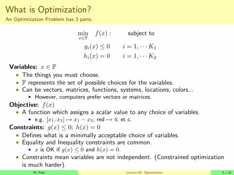
What is Optimization?An Optimization Problem has 3 parts.
minx∈F
f(x) : subject to
gi(x) ≤ 0 i = 1, · · ·K1
hi(x) = 0 i = 1, · · ·K2
Variables: x ∈ F• The things you must choose.• F represents the set of possible choices for the variables.• Can be vectors, matrices, functions, systems, locations, colors...
I However, computers prefer vectors or matrices.
Objective: f(x)• A function which assigns a scalar value to any choice of variables.
I e.g. [x1, x2] 7→ x1 − x2; red 7→ 4; et c.
Constraints: g(x) ≤ 0; h(x) = 0• Defines what is a minimally acceptable choice of variables.• Equality and Inequality constraints are common.
I x is OK if g(x) ≤ 0 and h(x) = 0.
• Constraints mean variables are not independent. (Constrained optimizationis much harder).
M. Peet Lecture 02: Optimization 2 / 31
Formulating Optimization ProblemsWhat do we need to know?
Topics to Cover:
Formulating Constraints
• Tricks of the Trade for expressing constraints.
• Converting everything to equality and inequality constraints.
Equivalence:
• How to Recognize if Two Optimization Problems are Equivalent.
• May be true despite different variables, constraints and objectives
Knowing which Problems are Solvable
• The Convex Ones.
• Some others, if the problem is relatively small.
M. Peet Lecture 02: Optimization 3 / 31
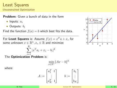
Least SquaresUnconstrained Optimization
Problem: Given a bunch of data in the form
• Inputs: ai
• Outputs: bi
Find the function f(a) = b which best fits the data.
For Least Squares is: Assume f(x) = xTa+ xc forsome unknown x ∈ Rn, xc ∈ R and minimize
K∑i=1
|xTai + xc − bi|2
The Optimization Problem is:
minx∈Rn‖Ax− b‖2
where
A :=
aT1 1...
aTK 1
b :=
b1...bK
M. Peet Lecture 02: Optimization 4 / 31
Least SquaresUnconstrained Optimization
Least squares problems are easy-ish to solve.
x = (ATA)−1AT b
Note that A is assumed to be skinny.
• More rows than columns.
• More data points than inputs.
M. Peet Lecture 02: Optimization 5 / 31
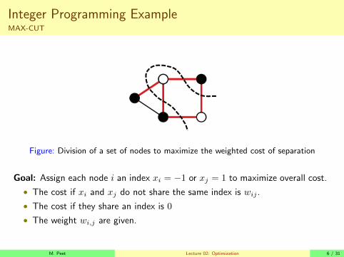
Integer Programming ExampleMAX-CUT
Figure: Division of a set of nodes to maximize the weighted cost of separation
Goal: Assign each node i an index xi = −1 or xj = 1 to maximize overall cost.
• The cost if xi and xj do not share the same index is wij .
• The cost if they share an index is 0
• The weight wi,j are given.
M. Peet Lecture 02: Optimization 6 / 31
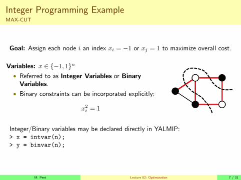
Integer Programming ExampleMAX-CUT
Goal: Assign each node i an index xi = −1 or xj = 1 to maximize overall cost.
Variables: x ∈ {−1, 1}n• Referred to as Integer Variables or Binary
Variables.
• Binary constraints can be incorporated explicitly:
x2i = 1
Integer/Binary variables may be declared directly in YALMIP:> x = intvar(n);
> y = binvar(n);
M. Peet Lecture 02: Optimization 7 / 31
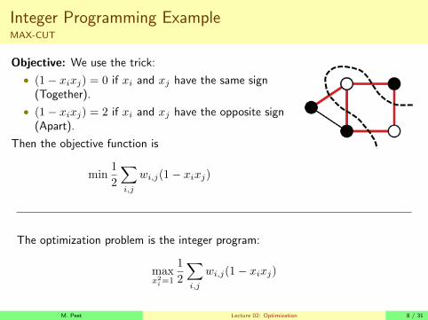
Integer Programming ExampleMAX-CUT
Objective: We use the trick:
• (1− xixj) = 0 if xi and xj have the same sign(Together).
• (1− xixj) = 2 if xi and xj have the opposite sign(Apart).
Then the objective function is
min1
2
∑i,j
wi,j(1− xixj)
The optimization problem is the integer program:
maxx2i=1
1
2
∑i,j
wi,j(1− xixj)
M. Peet Lecture 02: Optimization 8 / 31
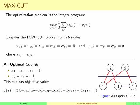
MAX-CUT
The optimization problem is the integer program:
maxx2i=1
1
2
∑i,j
wi,j(1− xixj)
Consider the MAX-CUT problem with 5 nodes
w12 = w23 = w45 = w15 = w34 = .5 and w14 = w24 = w25 = 0
where wij = wji.
An Optimal Cut IS:
• x1 = x3 = x4 = 1
• x2 = x5 = −1
This cut has objective value
f(x) = 2.5−.5x1x2−.5x2x3−.5x3x4−.5x4x5−.5x1x5 = 4
1
1
2
3 4
5
Figure: An Optimal Cut
M. Peet Lecture 02: Optimization 9 / 31
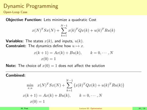
Dynamic ProgrammingOpen-Loop Case
Objective Function: Lets minimize a quadratic Cost
x(N)TSx(N) +
N−1∑k=1
x(k)TQx(k) + u(k)TRu(k)
Variables: The states x(k), and inputs, u(k).Constraint: The dynamics define how u 7→ x.
x(k + 1) = Ax(k) +Bu(k), k = 0, · · · , Nx(0) = 1
Note: The choice of x(0) = 1 does not affect the solution
Combined:
minx,u
x(N)TSx(N) +
N−1∑k=1
(x(k)TQx(k) + u(k)TRu(k)
)x(k + 1) = Ax(k) +Bu(k), k = 0, · · · , N
x(0) = 1
M. Peet Lecture 02: Optimization 10 / 31
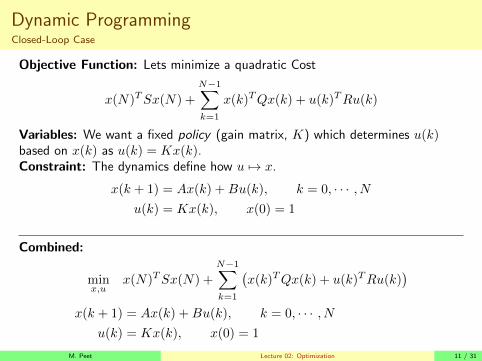
Dynamic ProgrammingClosed-Loop Case
Objective Function: Lets minimize a quadratic Cost
x(N)TSx(N) +
N−1∑k=1
x(k)TQx(k) + u(k)TRu(k)
Variables: We want a fixed policy (gain matrix, K) which determines u(k)based on x(k) as u(k) = Kx(k).Constraint: The dynamics define how u 7→ x.
x(k + 1) = Ax(k) +Bu(k), k = 0, · · · , Nu(k) = Kx(k), x(0) = 1
Combined:
minx,u
x(N)TSx(N) +
N−1∑k=1
(x(k)TQx(k) + u(k)TRu(k)
)x(k + 1) = Ax(k) +Bu(k), k = 0, · · · , N
u(k) = Kx(k), x(0) = 1
M. Peet Lecture 02: Optimization 11 / 31
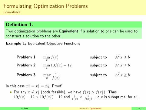
Formulating Optimization ProblemsEquivalence
Definition 1.
Two optimization problems are Equivalent if a solution to one can be used toconstruct a solution to the other.
Example 1: Equivalent Objective Functions
Problem 1: minxf(x) subject to ATx ≥ b
Problem 2: minx
10f(x)− 12 subject to ATx ≥ b
Problem 3: maxx
1
f(x)subject to ATx ≥ b
In this case x∗1 = x∗2 = x∗3. Proof:
• For any x 6= x∗1 (both feasible), we have f(x) > f(x∗1). Thus10f(x)− 12 > 10f(x∗1)− 12 and 1
f(x) <1
f(x∗1)
. i.e x is suboptimal for all.
M. Peet Lecture 02: Optimization 12 / 31
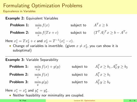
Formulating Optimization ProblemsEquivalence in Variables
Example 2: Equivalent Variables
Problem 1: minxf(x) subject to ATx ≥ b
Problem 2: minxf(Tx+ c) subject to (TTA)Tx ≥ b−AT c
Here x∗1 = Tx∗2 + c and x∗2 = T−1(x∗1 − c).• Change of variables is invertible. (given x 6= x∗2, you can show it is
suboptimal)
Example 3: Variable Separability
Problem 1: minx,y
f(x) + g(y) subject to AT1 x ≥ b1, AT2 y ≥ b2
Problem 2: minxf(x) subject to AT1 x ≥ b1
Problem 3: minyg(y) subject to AT2 y ≥ b2
Here x∗1 = x∗2 and y∗1 = y∗3 .• Neither feasibility nor minimality are coupled.
M. Peet Lecture 02: Optimization 13 / 31
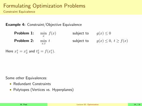
Formulating Optimization ProblemsConstraint Equivalence
Example 4: Constraint/Objective Equivalence
Problem 1: minx
f(x) subject to g(x) ≤ 0
Problem 2: minx,t
t subject to g(x) ≤ 0, t ≥ f(x)
Here x∗1 = x∗2 and t∗2 = f(x∗1).
Some other Equivalences:
• Redundant Constraints
• Polytopes (Vertices vs. Hyperplanes)
M. Peet Lecture 02: Optimization 14 / 31
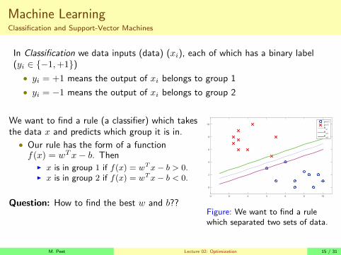
Machine LearningClassification and Support-Vector Machines
In Classification we data inputs (data) (xi), each of which has a binary label(yi ∈ {−1,+1})• yi = +1 means the output of xi belongs to group 1
• yi = −1 means the output of xi belongs to group 2
We want to find a rule (a classifier) which takesthe data x and predicts which group it is in.
• Our rule has the form of a functionf(x) = wTx− b. Then
I x is in group 1 if f(x) = wTx− b > 0.I x is in group 2 if f(x) = wTx− b < 0.
Question: How to find the best w and b??-2 0 2 4 6 8 10
0
2
4
6
8
10y=+1
y=-1
Hw
Hw1
Hw2
Figure: We want to find a rulewhich separated two sets of data.
M. Peet Lecture 02: Optimization 15 / 31
Machine LearningClassification and Support-Vector Machines
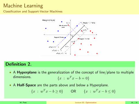
Definition 2.
• A Hyperplane is the generalization of the concept of line/plane to multipledimensions. {x : wTx− b = 0}
• A Half-Space are the parts above and below a Hyperplane.
{x : wTx− b ≥ 0} OR {x : wTx− b ≤ 0}
M. Peet Lecture 02: Optimization 16 / 31
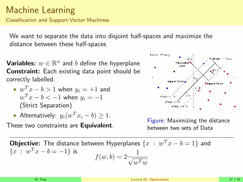
Machine LearningClassification and Support-Vector Machines
We want to separate the data into disjoint half-spaces and maximize thedistance between these half-spaces
Variables: w ∈ Rn and b define the hyperplaneConstraint: Each existing data point should becorrectly labelled.
• wTx− b > 1 when yi = +1 andwTx− b < −1 when yi = −1(Strict Separation)
• Alternatively: yi(wTxi − b) ≥ 1.
These two constraints are Equivalent.Figure: Maximizing the distancebetween two sets of Data
Objective: The distance between Hyperplanes {x : wTx− b = 1} and{x : wTx− b = −1} is
f(w, b) = 21√wTw
M. Peet Lecture 02: Optimization 17 / 31
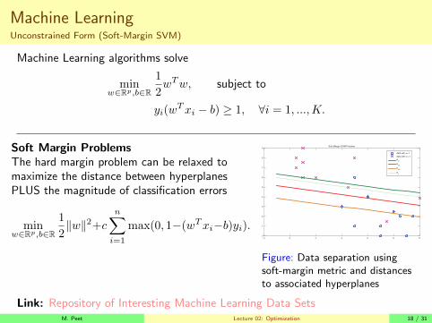
Machine LearningUnconstrained Form (Soft-Margin SVM)
Machine Learning algorithms solve
minw∈Rp,b∈R
1
2wTw, subject to
yi(wTxi − b) ≥ 1, ∀i = 1, ...,K.
Soft Margin ProblemsThe hard margin problem can be relaxed tomaximize the distance between hyperplanesPLUS the magnitude of classification errors
minw∈Rp,b∈R
1
2‖w‖2+c
n∑i=1
max(0, 1−(wTxi−b)yi).-2 0 2 4 6 8 10
0
1
2
3
4
5
6
7
8
9Soft Margin SVM Problem
data with y=-1
data with y=+1
Hw
Hw1
Hw2
Hξ
Figure: Data separation usingsoft-margin metric and distancesto associated hyperplanes
Link: Repository of Interesting Machine Learning Data SetsM. Peet Lecture 02: Optimization 18 / 31
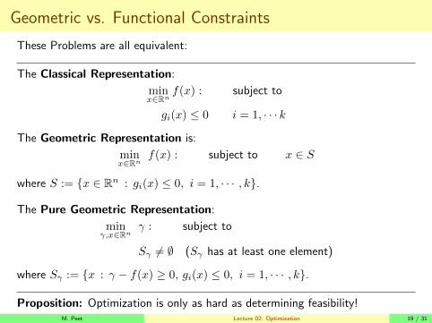
Geometric vs. Functional Constraints
These Problems are all equivalent:
The Classical Representation:
minx∈Rn
f(x) : subject to
gi(x) ≤ 0 i = 1, · · · k
The Geometric Representation is:
minx∈Rn
f(x) : subject to x ∈ S
where S := {x ∈ Rn : gi(x) ≤ 0, i = 1, · · · , k}.
The Pure Geometric Representation:
minγ,x∈Rn
γ : subject to
Sγ 6= ∅ (Sγ has at least one element)
where Sγ := {x : γ − f(x) ≥ 0, gi(x) ≤ 0, i = 1, · · · , k}.
Proposition: Optimization is only as hard as determining feasibility!M. Peet Lecture 02: Optimization 19 / 31
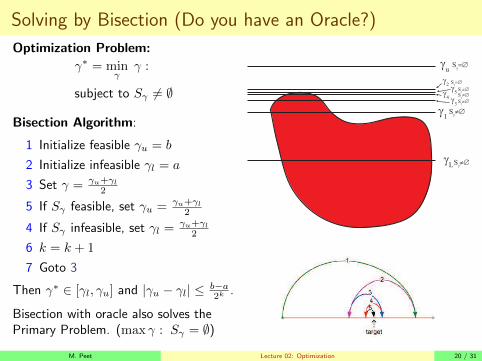
Solving by Bisection (Do you have an Oracle?)
Optimization Problem:
γ∗ = minγ
γ :
subject to Sγ 6= ∅
Bisection Algorithm:
1 Initialize feasible γu = b
2 Initialize infeasible γl = a
3 Set γ = γu+γl2
5 If Sγ feasible, set γu = γu+γl2
4 If Sγ infeasible, set γl = γu+γl2
6 k = k + 1
7 Goto 3
Then γ∗ ∈ [γl, γu] and |γu − γl| ≤ b−a2k
.
Bisection with oracle also solves thePrimary Problem. (max γ : Sγ = ∅)
γL
γu
γ1
γ2
Sγ=∅
γ4 γ
3
Sγ≠∅
Sγ≠∅
γ5
Sγ=∅
Sγ≠∅
Sγ≠∅
Sγ≠∅
M. Peet Lecture 02: Optimization 20 / 31
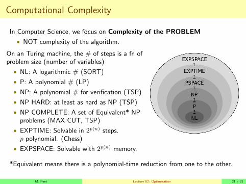
Computational Complexity
In Computer Science, we focus on Complexity of the PROBLEM
• NOT complexity of the algorithm.
On an Turing machine, the # of steps is a fn ofproblem size (number of variables)
• NL: A logarithmic # (SORT)
• P: A polynomial # (LP)
• NP: A polynomial # for verification (TSP)
• NP HARD: at least as hard as NP (TSP)
• NP COMPLETE: A set of Equivalent* NPproblems (MAX-CUT, TSP)
• EXPTIME: Solvable in 2p(n) steps.p polynomial. (Chess)
• EXPSPACE: Solvable with 2p(n) memory.
*Equivalent means there is a polynomial-time reduction from one to the other.
M. Peet Lecture 02: Optimization 21 / 31
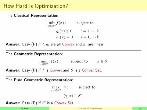
How Hard is Optimization?
The Classical Representation:
minx∈Rn
f(x) : subject to
gi(x) ≤ 0 i = 1, · · · khi(x) = 0 i = 1, · · · k
Answer: Easy (P) if f, gi are all Convex and hi are linear.
The Geometric Representation:
minx∈Rn
f(x) : subject to x ∈ S
Answer: Easy (P) if f is Convex and S is a Convex Set.
The Pure Geometric Representation:
maxγ,x∈Rn
γ : subject to
(γ, x) ∈ S′
Answer: Easy (P) if S′ is a Convex Set.M. Peet Lecture 02: Optimization 22 / 31
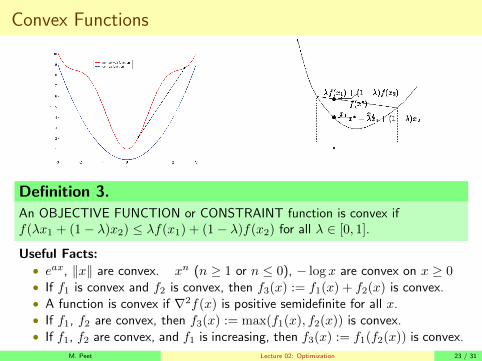
Convex Functions
Definition 3.
An OBJECTIVE FUNCTION or CONSTRAINT function is convex iff(λx1 + (1− λ)x2) ≤ λf(x1) + (1− λ)f(x2) for all λ ∈ [0, 1].
Useful Facts:• eax, ‖x‖ are convex. xn (n ≥ 1 or n ≤ 0), − log x are convex on x ≥ 0• If f1 is convex and f2 is convex, then f3(x) := f1(x) + f2(x) is convex.• A function is convex if ∇2f(x) is positive semidefinite for all x.• If f1, f2 are convex, then f3(x) := max(f1(x), f2(x)) is convex.• If f1, f2 are convex, and f1 is increasing, then f3(x) := f1(f2(x)) is convex.
M. Peet Lecture 02: Optimization 23 / 31
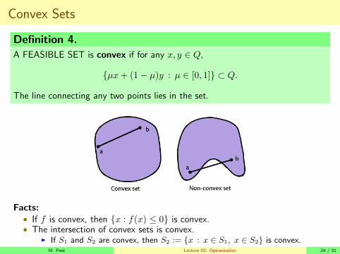
Convex Sets
Definition 4.
A FEASIBLE SET is convex if for any x, y ∈ Q,
{µx+ (1− µ)y : µ ∈ [0, 1]} ⊂ Q.
The line connecting any two points lies in the set.
Facts:• If f is convex, then {x : f(x) ≤ 0} is convex.• The intersection of convex sets is convex.
I If S1 and S2 are convex, then S2 := {x : x ∈ S1, x ∈ S2} is convex.M. Peet Lecture 02: Optimization 24 / 31
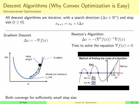
Descent Algorithms (Why Convex Optimization is Easy)Unconstrained Optimization
All descent algorithms are iterative, with a search direction (∆x ∈ Rn) and stepsize (t ≥ 0). xk+1 = xk + t∆x
Gradient Descent
∆x = −∇f(x)
Newton’s Algorithm:
∆x = −(∇2f(x))−1∇f(x)
Tries to solve the equation ∇f(x) = 0.
Both converge for sufficiently small step size.M. Peet Lecture 02: Optimization 25 / 31
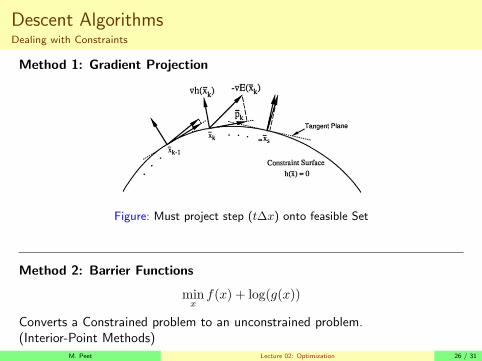
Descent AlgorithmsDealing with Constraints
Method 1: Gradient Projection
Figure: Must project step (t∆x) onto feasible Set
Method 2: Barrier Functions
minxf(x) + log(g(x))
Converts a Constrained problem to an unconstrained problem.(Interior-Point Methods)
M. Peet Lecture 02: Optimization 26 / 31
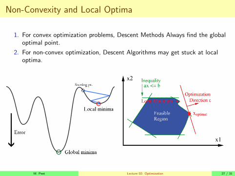
Non-Convexity and Local Optima
1. For convex optimization problems, Descent Methods Always find the globaloptimal point.
2. For non-convex optimization, Descent Algorithms may get stuck at localoptima.
M. Peet Lecture 02: Optimization 27 / 31
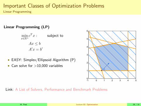
Important Classes of Optimization ProblemsLinear Programming
Linear Programming (LP)
minx∈Rn
cTx : subject to
Ax ≤ bA′x = b′
• EASY: Simplex/Ellipsoid Algorithm (P)
• Can solve for >10,000 variables
2 - 13 Convexity and Duality S. Lall, Stanford 2004.08.30.01
Linear Programming (LP)
In a linear program, the objective and constraint functions are affine.
minimize cTx
subject to Ax = b
Cx ≤ d
Example
minimize x1 + x2
subject to 3x1 + x2 ≥ 3
x2 ≥ 1
x1 ≤ 4
−x1 + 5x2 ≤ 20
x1 + 4x2 ≤ 20
Link: A List of Solvers, Performance and Benchmark Problems
M. Peet Lecture 02: Optimization 28 / 31
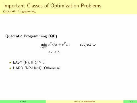
Important Classes of Optimization ProblemsQuadratic Programming
Quadratic Programming (QP)
minx∈Rn
xTQx+ cTx : subject to
Ax ≤ b
• EASY (P): If Q ≥ 0.
• HARD (NP-Hard): Otherwise
M. Peet Lecture 02: Optimization 29 / 31
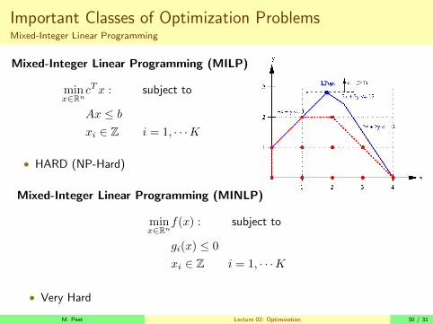
Important Classes of Optimization ProblemsMixed-Integer Linear Programming
Mixed-Integer Linear Programming (MILP)
minx∈Rn
cTx : subject to
Ax ≤ bxi ∈ Z i = 1, · · ·K
• HARD (NP-Hard)
Mixed-Integer Linear Programming (MINLP)
minx∈Rn
f(x) : subject to
gi(x) ≤ 0
xi ∈ Z i = 1, · · ·K
• Very Hard
M. Peet Lecture 02: Optimization 30 / 31

Next Time:
Positive Matrices, SDP and LMIs
• Also a bit on Duality, Relaxations.
M. Peet Lecture 02: Optimization 31 / 31