literature survey: e-elt under control - tu delftmverhaegen/n4ci/publications/wklop_msc... · e-elt...
TRANSCRIPT

Delft Center for Systems and Control
E-ELT under controlAdaptive optics low-level control solution for E-ELT
W.A. Klop
Lit
eratu
reSurv
ey


E-ELT under controlAdaptive optics low-level control solution for E-ELT
Literature Survey
W.A. Klop
May 26, 2011
Faculty of Faculteit Elektrotechniek, Wiskunde en Informatica (EWI) · Delft University ofTechnology

Copyright c©All rights reserved.

Abstract
Scientist are building increasingly larger telescopes and this is not only influencing the me-chanical structure. An adaptive optics (AO) system is an essential instrument installed inlarge telescopes to prevent blurry images. The wavefront reconstructor is an component ofthe AO control process. When N defines the number of actuators, then the computationaleffort to calculate the wavefront reconstructor scales with the order O(N2) for standard vec-tor matrix multiply (VMM) methods. For the class of extremely large telescope (ELT)s nowunder consideration these calculation become infeasible. Extensive research is already doneon how to lower the order of wavefront reconstruction algorithms. However, expected is thatlowering the order is not sufficient, emphasising the need for optimisation on all the levels ofimplementation. The parallel computing concept seems to be a excellent contender to furtherimprove the performance on the level off hardware implementation. The link connecting thealgorithms and the hardware lies in the conditions imposed on each technology that allows itto work effectively. During the research the conditions and properties of the different tech-nologies were evaluated. Analysing to which extend there exists cohesion between a particularalgorithm and hardware platform. From the three algorithms under consideration they allare suitable till a certain extend. The structured Kalman method excels with respect toperformance and accuracy. However the parallel computing concept requires independencyamong data, preferable at a high level to achieve optimal performance. This aspect lacksin all three algorithms. Recommended is to perform additional research on the redesign orredevelopment of algorithms to fit better the parallel computing profile. Also is suggestedto explore the option of a localised approach where only nearest-neighbour information isutilised to estimate a phase difference of a single segment.
Literature Survey W.A. Klop

ii
W.A. Klop Literature Survey

Table of Contents
Preface & Acknowledgements ix
1 Introduction 1
1-1 Telescopes . . . . . . . . . . . . . . . . . . . . . . . . . . . . . . . . . . . . . . 1
1-2 Adaptive optics in astronomy . . . . . . . . . . . . . . . . . . . . . . . . . . . . 2
1-3 Computational explosion . . . . . . . . . . . . . . . . . . . . . . . . . . . . . . 3
1-4 Outline . . . . . . . . . . . . . . . . . . . . . . . . . . . . . . . . . . . . . . . . 4
2 Parallel Computing 5
2-1 General Aspects . . . . . . . . . . . . . . . . . . . . . . . . . . . . . . . . . . . 5
2-1-1 Background . . . . . . . . . . . . . . . . . . . . . . . . . . . . . . . . . 5
2-1-2 Basic Concepts . . . . . . . . . . . . . . . . . . . . . . . . . . . . . . . 6
2-2 Case Study . . . . . . . . . . . . . . . . . . . . . . . . . . . . . . . . . . . . . . 8
2-2-1 Fine grained approach . . . . . . . . . . . . . . . . . . . . . . . . . . . . 9
2-2-2 Coarse grained approach . . . . . . . . . . . . . . . . . . . . . . . . . . 9
3 Parallel processors 11
3-1 Development . . . . . . . . . . . . . . . . . . . . . . . . . . . . . . . . . . . . . 11
3-2 Architecture . . . . . . . . . . . . . . . . . . . . . . . . . . . . . . . . . . . . . 12
3-3 Applicability . . . . . . . . . . . . . . . . . . . . . . . . . . . . . . . . . . . . . 14
3-3-1 Overview . . . . . . . . . . . . . . . . . . . . . . . . . . . . . . . . . . . 16
4 Reconfigurable Computing 17
4-1 Development . . . . . . . . . . . . . . . . . . . . . . . . . . . . . . . . . . . . . 17
4-2 Architecture . . . . . . . . . . . . . . . . . . . . . . . . . . . . . . . . . . . . . 18
4-3 Applicability . . . . . . . . . . . . . . . . . . . . . . . . . . . . . . . . . . . . . 20
4-3-1 Overview . . . . . . . . . . . . . . . . . . . . . . . . . . . . . . . . . . . 21
Literature Survey W.A. Klop

iv Table of Contents
5 Adaptive Optics Algorithms 23
5-1 Fast Fourier transform reconstruction . . . . . . . . . . . . . . . . . . . . . . . . 23
5-1-1 General Info . . . . . . . . . . . . . . . . . . . . . . . . . . . . . . . . . 23
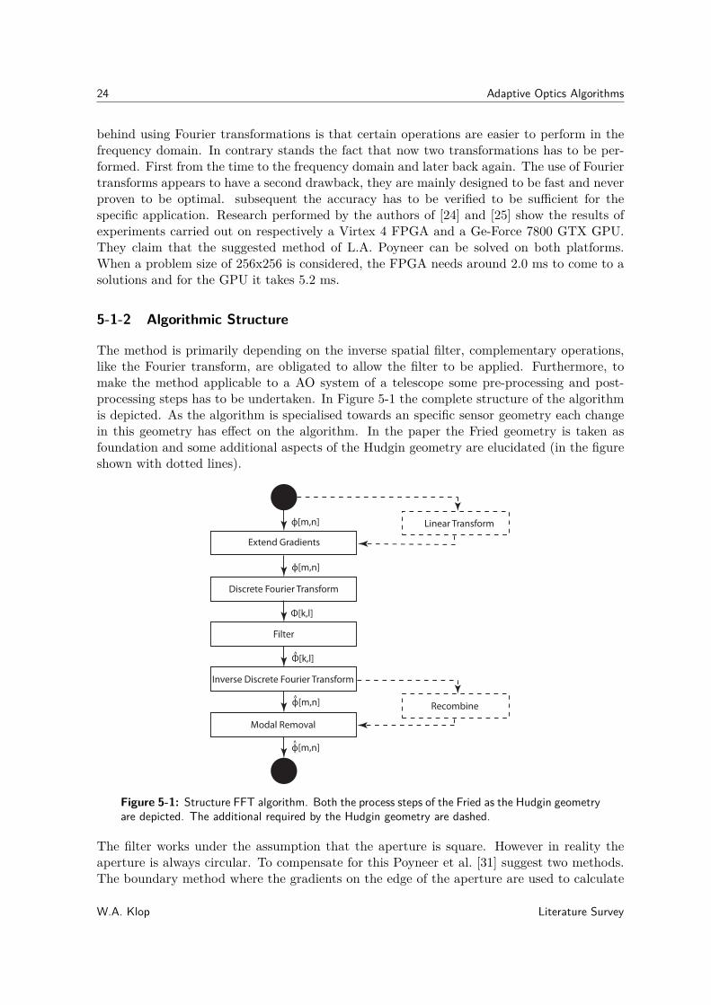
5-1-2 Algorithmic Structure . . . . . . . . . . . . . . . . . . . . . . . . . . . . 24
5-1-3 Analysis . . . . . . . . . . . . . . . . . . . . . . . . . . . . . . . . . . . 25
5-2 Sparse minimum variance reconstruction . . . . . . . . . . . . . . . . . . . . . . 27
5-2-1 General Info . . . . . . . . . . . . . . . . . . . . . . . . . . . . . . . . . 27
5-2-2 Algorithmic Structure . . . . . . . . . . . . . . . . . . . . . . . . . . . . 28
5-2-3 Analysis . . . . . . . . . . . . . . . . . . . . . . . . . . . . . . . . . . . 28
5-3 Structured Kalman reconstruction . . . . . . . . . . . . . . . . . . . . . . . . . 30
5-3-1 General Info . . . . . . . . . . . . . . . . . . . . . . . . . . . . . . . . . 30
5-3-2 Algorithmic Structure . . . . . . . . . . . . . . . . . . . . . . . . . . . . 30
5-3-3 Analysis . . . . . . . . . . . . . . . . . . . . . . . . . . . . . . . . . . . 31
5-4 Overview . . . . . . . . . . . . . . . . . . . . . . . . . . . . . . . . . . . . . . . 32
6 Findings 35
6-1 Conclusions . . . . . . . . . . . . . . . . . . . . . . . . . . . . . . . . . . . . . 35
6-2 Recommendations . . . . . . . . . . . . . . . . . . . . . . . . . . . . . . . . . . 36
6-3 Project Proposal . . . . . . . . . . . . . . . . . . . . . . . . . . . . . . . . . . . 37
A Additional Algorithm details 39
A-1 Fast Fourier transform reconstruction . . . . . . . . . . . . . . . . . . . . . . . . 39
A-2 Sparse minimum variance reconstruction . . . . . . . . . . . . . . . . . . . . . . 41
A-3 Structured Kalman reconstruction . . . . . . . . . . . . . . . . . . . . . . . . . 41
Bibliography 43
Glossary 47
List of Acronyms . . . . . . . . . . . . . . . . . . . . . . . . . . . . . . . . . . . 47
List of Symbols . . . . . . . . . . . . . . . . . . . . . . . . . . . . . . . . . . . 48
W.A. Klop Literature Survey

List of Figures
1-1 Schematic representation of a Adaptive Optics system . . . . . . . . . . . . . . . 2
1-2 Interweaved process of optimising a system design . . . . . . . . . . . . . . . . . 4
2-1 Degradation of speedup by Amdahl’s law. Sp is a function of (α) the fraction ofnon-parallelizable code. . . . . . . . . . . . . . . . . . . . . . . . . . . . . . . . 7
3-1 Architecture overview of GPU [30] . . . . . . . . . . . . . . . . . . . . . . . . . 13
3-2 Programming model of a the GPU programming language CUDA . . . . . . . . . 14
4-1 Simple representation of a logic block . . . . . . . . . . . . . . . . . . . . . . . 19
4-2 Architecture of FPGA . . . . . . . . . . . . . . . . . . . . . . . . . . . . . . . . 20
5-1 Structure FFT algorithm. Both the process steps of the Fried as the Hudgingeometry are depicted. The additional required by the Hudgin geometry are dashed. 24
5-2 Wavefront reconstruction algorithm . . . . . . . . . . . . . . . . . . . . . . . . . 30
5-3 SSS matrix-vector multiplication as a series of subsystems . . . . . . . . . . . . 31
6-1 Graduation project proposal . . . . . . . . . . . . . . . . . . . . . . . . . . . . . 37
Literature Survey W.A. Klop

vi List of Figures
W.A. Klop Literature Survey
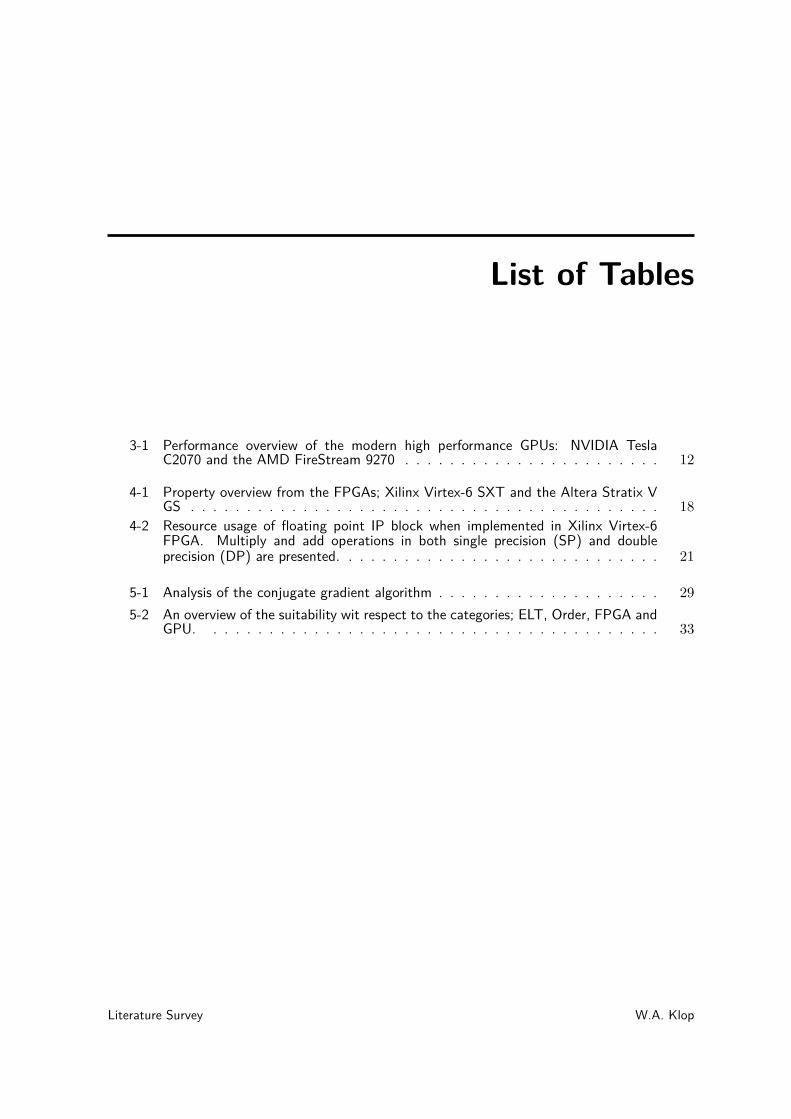
List of Tables
3-1 Performance overview of the modern high performance GPUs: NVIDIA TeslaC2070 and the AMD FireStream 9270 . . . . . . . . . . . . . . . . . . . . . . . 12
4-1 Property overview from the FPGAs; Xilinx Virtex-6 SXT and the Altera Stratix VGS . . . . . . . . . . . . . . . . . . . . . . . . . . . . . . . . . . . . . . . . . . 18
4-2 Resource usage of floating point IP block when implemented in Xilinx Virtex-6FPGA. Multiply and add operations in both single precision (SP) and doubleprecision (DP) are presented. . . . . . . . . . . . . . . . . . . . . . . . . . . . . 21
5-1 Analysis of the conjugate gradient algorithm . . . . . . . . . . . . . . . . . . . . 29
5-2 An overview of the suitability wit respect to the categories; ELT, Order, FPGA andGPU. . . . . . . . . . . . . . . . . . . . . . . . . . . . . . . . . . . . . . . . . 33
Literature Survey W.A. Klop

viii List of Tables
W.A. Klop Literature Survey
Preface & Acknowledgements
The Literature Study is an element of the graduation process. The document at hand de-scribes the findings I discovered during my research. The first step in the graduation process isselecting a topic. My personal preference of graduating within the Technical University led metowards the subject. After a consultation with Micheal Verheagen and Rufus Fraanje a globalidea was defined. Finally the idea was refined and with this the subject became; Low levelcontrol of adaptive optics (AO) systems in relation with extremely large telescope (ELT)s.During the Literature Study I concerned myself with the issues related to a specific elementof AO control. The implementation of the wavefront reconstruction process. To keep myresearch on track a received frequent supervision of my daily supervisor, Rufus Fraanje. Foradditional counsel I was able to discuss my problems with Professor Michel Verhaegen.
Delft, University of Technology W.A. KlopMay 26, 2011
Literature Survey W.A. Klop

x Preface & Acknowledgements
W.A. Klop Literature Survey

“People asking questions, lost in confusion, well I tell them there’s no problem,only solutions.”
— John Lennon —


Chapter 1
Introduction
Exploring is a essential component of the human character, as long as we exist we are won-dering what the stars in the universe will bring us. To find some answers we are building awide variety of instrumentation. One of the most important ground-based instruments forastronomers is the telescope. Driven by our curiosity we are constructing increasingly largertelescopes. We are now arrived at the era of the extremely large telescope (ELT). This is aclass of telescopes where the aperture exceeds the 20 meter range. Constructing telescopesfrom this kind of magnitudes comes with numerous challenges. Controlling the AdaptiveOptics systems is one of these challenges which will be addressed in this document.
1-1 Telescopes
With the invention of the telescope in 1608 [35] it became possible to study the universe inmuch more detail. In contrast to the only possible way till then: the naked eye. The firsttelescope existed of an objective and ocular, also referred to as a refractor based telescope.The growth in diameter of the telescopes required another type of design. A new designbased on a curved mirror was suggested by Isaac Newton in 1668. Despite the theoreticaladvantages, production technologies held back the introduction of the reflecting telescopetill the 18th century. All current astronomical telescopes are based on reflective designs.Increasing the diameter of the telescopes is driven by two important properties in any opticalimaging system: the light collecting power and the angular resolution. Where the Rayleighcriterion gives an estimate of the angular resolution and is defined by
sinθ ≈ 1.22λ
D(1-1)
Where λ is the wavelength of the light emitted by the object that is observed, D definesthe diameter of the aperture and θ gives the angular resolution. The smaller the angularresolution the more detail can be observed. Eq. (1-1) results in the fact that by increasingD the angular resolution will improve. Nowadays this makes us believe that an extremely
Literature Survey W.A. Klop

2 Introduction
large telescope (ELT) can deliver an important contribution to our astronomical knowledge.Several of this type of ELT‘s are planned to be build in the coming decade. Among them arethe astronomers of European Southern Observatory (ESO) who are designing the Europeanversion of an ELT since 2005.
1-2 Adaptive optics in astronomy
There is an issue that has to be resolved to be able to use the full extent of an ELT. When thediameter of the telescope is enlarged beyond approximately 0.2 meter the angular resolutionin no longer diffraction limited, but seeing limited. Caused by turbulence in the earth’satmosphere. Each ground-based telescope has to pass the earth’s atmosphere to retrieve theimage. The light travelling through this atmosphere gets distorted caused by temperaturedifferences, resulting in a blurry image. A solution would be to place the telescope outsidethe earth’s atmosphere as was done with the Hubble telescope. Two major disadvantagesthat come with this solution is the inability to do rapid maintenance or repair and of coursethe extreme costs related to such a telescope. Another critical limitation is the size of thetelescope. Bigger is advantageous for the light collecting power. However travelling to spaceis still complicated and does not allow for large payloads.
Turbule
nce
Plane w
avefront
Disturb
ed wavefro
nt
Tele
scope
Beam splitterWavefront sensor
Scienti!c camera
Controller
Deform
able M
irror
Observ
ed obje
ct
s(.)
u(.)
Figure 1-1: Schematic representation of a Adaptive Optics system
W.A. Klop Literature Survey
1-3 Computational explosion 3
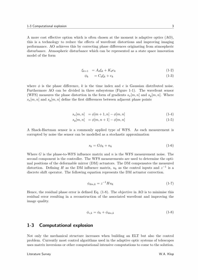
A more cost effective option which is often chosen at the moment is adaptive optics (AO),this is a technology to reduce the effects of wavefront distortions and improving imagingperformance. AO achieves this by correcting phase differences originating from atmosphericdisturbance. Atmospheric disturbance which can be represented as a state space innovationmodel of the form
ξk+1 = Adξk + Kdek (1-2)
φk = Cdξk + ek (1-3)
where φ is the phase difference, k is the time index and e is Gaussian distributed noise.Furthermore AO can be divided in three subsystems (Figure 1-1). The wavefront sensor(WFS) measures the phase distortion in the form of gradients sx[m, n] and sy[m, n]. Wheresx[m, n] and sy[m, n] define the first differences between adjacent phase points
sx[m, n] = φ[m + 1, n]− φ[m, n] (1-4)
sy[m, n] = φ[m, n + 1]− φ[m, n] (1-5)
A Shack-Hartman sensor is a commonly applied type of WFS. As each measurement iscorrupted by noise the sensor can be modelled as a stochastic approximation
sk = Gφk + nk (1-6)
Where G is the phase-to-WFS influence matrix and n is the WFS measurement noise. Thesecond component is the controller. The WFS measurements are used to determine the opti-mal positions of the deformable mirror (DM) actuators. The DM compensates the measureddistortion. Defining H as the DM influence matrix, uk as the control inputs and z−1 is adiscrete shift operator. The following equation represents the DM actuator correction.
φdm,k = z−1Huk (1-7)
Hence, the residual phase error is defined Eq. (1-8). The objective in AO is to minimise thisresidual error resulting in a reconstruction of the associated wavefront and improving theimage quality.
φε,k = φk + φdm,k (1-8)
1-3 Computational explosion
Not only the mechanical structure increases when building an ELT but also the controlproblem. Currently most control algorithms used in the adaptive optic systems of telescopesuses matrix inversions or other computational intensive computations to come to the solution.
Literature Survey W.A. Klop

4 Introduction
Till now these methods were no issue. With the increasing size of the mirror also the number ofWFS segments and the DM actuators increased. Keeping in mind the limit of approximately0.2 meter for which telescopes are still diffraction limited. Resulting for the E-ELT in a totalamount of actuators (n) that is expected to exceed the 40.000. Making an algorithm withorder O(n2) or higher is not acceptable anymore. Already huge amount of research is doneto more efficient algorithms. Even with these more efficient algorithms it is expected thatsolving the control problem is still not feasible in real-time considering current performancelevels and Moore’s law [11]. Each scientific problem can be optimised at several levels, alreadythe top level has to be addressed. Also the lower levels can be improved, each algorithm canbe converted to software in several ways, optimised for different hardware platforms. Notethat software and hardware are tightly interconnected, changing the hardware often resultsin software changes. Even further, preference on the selected hardware can also influence thealgorithm design or the other way around. Making the total system design from algorithmtill hardware a complex interweaved process (Figure 1-2).
Algorithm design
Software implementation Hardware platform
Figure 1-2: Interweaved process of optimising a system design
1-4 Outline
Already some experiments emphasising on the AO implementation with respect to ELTs werepublished. In [34] 16 Nvidia 8800 ultra fast graphics processing units (GPU) distributed over8 dual core HP Optron computers are used to solve a 64 × 64 sized AO problem. Applyingregular VMM methods they achieve a framerate of 2 kHz. Similar, in [19] 9 boards containingsix field programmable gate array (FPGA)s each controlled by two general purpose computerboards packed with three Intel L7400 dual core processors solve approximately a 86×86 sizedAO problem. In this case a conjugate gradient method is utilised to achieve a framerate of 800Hz. Both options succeed for the given problem, however they are relatively small compared tothe ELT related AO problem. Predicting whether the suggested designs are sufficient requiresknowledge about bottlenecks related to technologies. This document describes issues andproperties for both the technologies, as well for some algorithms. Allowing for the estimationof critical bottlenecks and in addition guiding towards a possible strategy. Chapter 2 explainsthe parallel computing concept. Dealing with the main aspects around parallel algorithmsimplementations. Chapter 3 considers parallel processors. Explicitly pointing out GPUs byaddressing its advantages and disadvantages. Chapter 4 discusses reconfigurable computing.Where FPGA technology is considered as a potential candidate. Chapter 5 focusses on theAO algorithms, more accurate on the wavefront reconstruction component. Each of the threediscussed algorithms is analysed for performance, accuracy and the expected success factorwhen mapped to a parallel version. Chapter 6 finishes the discussion with conclusions andrecommendations based on the findings of the previous chapters. Also a proposal for thegraduation project is given.
W.A. Klop Literature Survey

Chapter 2
Parallel Computing
Engineering often consist of making tradeoffs. Parallel computing is such a tradeoff, thistechnology trades space for time. Traditionally algorithms are performed sequentially. Forscientific problems this approach is often impractical. The time it would take, before theresults will be available can be enormous. Parallel computing addresses this issue and insteadof executing the steps sequential the idea is to perform them simultaneous or in parallel.Related to the technology used to make the calculations known as integrated circuits, thismeans that available die area is used to solve the problem in a shorter time window. Especiallyin the case of real-time problems where time is sparse, like the AO systems in telescopes,problems can benefit from parallel computing technology.
2-1 General Aspects
2-1-1 Background
Usually when a problem has to be solved an algorithm is developed and then implemented in asequential set of instructions. The execution of the instructions finds place on a single process-ing unit. The unit is executing one instruction at a time, after the first instruction is finishedthe next is started. This cycle keeps going till the algorithm is finished. The concept is easilycomprehensible for programmers and as such it is straightforward to apply. This makes it anattractive option. On the other side we find parallel computing. This technology uses multi-ple processing units to work simultaneously on the same problem. To accomplish parallelismthe algorithm has to be broken up into several independent subproblems. These subproblemsthen can be dived over the multiple processing units. Parallel computing is already a wellestablish field for a while and its primary domain of interest was high-performance computing,however this is shifting since physical limitations are preventing frequency scaling. Frequencyscaling was from around 1985 till 2004 the dominant method used by IC manufactures toincrease the performance. The execution time of a program can be determined by countingthe number of instructions and multiplying this by the average time each instructions needs.
Literature Survey W.A. Klop

6 Parallel Computing
A way to decrease the average instruction execution time is by increasing the clock frequencyof the processing unit. Resulting in a lower execution time of the overall program. Thisargument gave plenty of reason for manufacturers to let frequency scaling be the dominantdesign parameter. As already mentioned earlier this method became infeasible to hold asdominant design parameter. Power consumption is the fundamental reason for the ceasingenhance in frequency scaling. The power consumption of an IC is defined as Eq. (2-1) in [18,p. 18].
P =1
2CV 2F, (2-1)
Where C is the capacitance switched per clock cycle. V is the supply voltage and F isthe frequency the IC is driven by. The equation shows directly the problem, increasing thefrequency will also increase the power consumption, if both the capacitance and the voltageare kept equal. Since also the voltage was reduced from 5 volt till 1 volt over the past 20 yearssome additional headroom was available. Slowly physical limitations were emerging. Burningvast amounts of power meant that temperature were rising to unacceptable levels. Gordon E.Moore made the observation that since the invention of the IC that the number of componentsin IC’s doubled every year [26]. Moore also predicted that this trend would carry on, nowadaysreferred to as Moore’s Law. Later on Moore refined the law and changed the period into twoyears. Till now Moore’s law it still valid. From the beginning these new available resourceswere used to support higher frequencies. Since frequency scaling is no longer the dominantdesign parameter these components can be used for other purposes. Manufacturers are nowaiming at increasingly larger numbers of cores favouring parallel computing.
2-1-2 Basic Concepts
When applying parallelism the design is dictated by the speed-up factor. The speed-up factoris defined by the relation between the algorithms original execution time and the executiontime of the redesigned version.
Sp =Eold
Enew=
1
(1− F ) + FSp(enhanced)
(2-2)
Where Sp is the overall speed-up factor, Eold and Enew are the execution times of respectivelythe task without and with enhancement, F is the fraction of code, that could be enhancedand Sp(enhanced) is the speedup factor of the enhanced code. Ideally the speed-up factor wouldbe linear with respect to parallel computing, meaning that when the number of processingunits increases the runtime decreases with the same factor. However, in practise this is almostnever achievable. Several different issues play a role. The section of the algorithm that allowsto be parallelized can have a major impact. Gene Amdalh observed this and formulated thepotential speed-up factor on a parallel computing platform in Amdalh’s Law [15, p. 66]. Thelaw states that the speed-up of a program is dictated by the section of the algorithm whichcannot be parallelized. The resulting fact is that the sequential part will finally determine theruntime. In case of a realistic scientific problem, which will often exists of both parallelizableand sequential parts, this has a significant influence on the runtime. The relationship definedby Amdalh’s Law is formulated as
W.A. Klop Literature Survey

2-1 General Aspects 7
Sp =1
α + (1−α)p
(2-3)
Where α is the fraction of the code that is non-parallelizable and p is the number of processingunits. Putting the law in perspective: if for example 50 percent of the code cannot beparallelized, the maximal achievable speed-up will be 2x regardless of the number of processorsadded. The effect is shown in Figure 2-3, the number of processing units chosen here is 10 andthe sequential portion is 50 %. The effect described by Amdahl’s law will limit the usefulnessoff augmenting processing units.
0 0.2 0.4 0.6 0.8 11
2
3
4
5
6
7
8
9
10
a
Sp
Amdahl’s Law
Figure 2-1: Degradation of speedup by Amdahl’s law. Sp is a function of (α) the fraction ofnon-parallelizable code.
Data dependency or rather independency is the critical parameter in parallelism. Depen-dency in this context is the case where prior calculations have to be completed before thealgorithm can proceed. The largest set of uninterrupted dependent instructions defines thecritical path. The optimisation of an algorithm by parallelizing is limited to the runtime ofthe critical path. An example of a human analog to the critical path was called by FredBrooks in [5]. It states "Nine women can’t make a baby in one month". The same applies tocertain sections of algorithms.parallelizing algorithms can be performed at different levels. On an elementary operationlevel this is referred to as fine grained. Or on a level where a complete set of elementary oper-ations form a subproblem, this is defined as coarse grained. Often it is more straightforwardto parallelize on a fine grained level like matrix multiplications. There are often fewer datadependencies and certainly the insight in the functioning is better. However how temptingthis may be, when feasible it will be better to follow the coarse grained approach.Communication in the field of processing unit is expensive. When communicating the pro-cessing units have to use the memory to share their temporal results. Memory access is slowcompared to the processing unit, causing the processing unit to stall. Communication is alsoseen as overhead since the calculation is the primary objective. The less communication, the
Literature Survey W.A. Klop

8 Parallel Computing
better. Knowing this argument, the advantage of coarse grained is quite obvious. When eachprocessing unit can progress without intervention for a longer period of time the reducedcommunication will benefit the overall speedup.Amdahls law assumes that the part that can be made parallel can be infinitely speed-up justby increasing the number of processing units. In practise, the observation will be that as soonas a certain number of processing units is reached, the speed-up factor will decline. In thebook "The mythical man month" [5] this effect is also revealed with relation to late softwaredevelopment projects. Keep adding man power will not help to get the project finished intime and eventually will have a negative impact. The main cause is again the overhead ofcommunication that increases, when then number of people working on a project is increasing.At a particular point meetings will dominate the time spend on a project. There is a largecoherence to parallel computing, the only difference lies in the fact that people are replacedby processing units.Load balancing plays another decisive role in the difference between the theoretical and prac-tical speed up factor. Hardware comes frequently with a fixed number of processing units.When the algorithm is split up, the resulting number of subsections does not always matchthe number of processing units defined by the hardware. In case of insufficient subsections, itmeans that several processing units will be idle. In the opposite case when there are to muchsubsections, they have to split up in two groups. First executing one group followed by thenext. In either case there is a inconsistency in comparison to the theoretical feasible upperlimit.The hardware architecture has impact on how an algorithm is converted to a parallel version.Michael J. Flynn [12] was one of the first to define a classification for computation plat-forms. The two classes which are interesting in relation to parallel computing are the singleinstruction multiple data (SIMD) and multiple instruction multiple data (MIMD). SIMD hasthe same control logic for different processing units, this means that it performs the sameinstruction on distinct data. An advantage is that there is less die area required for the logicunit, making space available for more or advanced processing units. Opposite to SIMD standsMIMD, These types of hardware platforms have its own control unit for each processing unit.Allowing to perform different instructions on different data set creating a set of completelyindependent processing units. Providing much more flexibility in contrast to SIMD. Bothtechnologies have their advantages and specific application area’s. For example the MIMDarchitecture is applied in current multi-core CPU technology. Where the SIMD architecturecan be recognised in GPU hardware designs.
2-2 Case Study
To show the difference between a fine grained and a coarse grained approach an example caseis defined. The case is selected for its ability to fit for both approaches and has no directresemblance with reality. Assume we have a square grid of 16 x 16 sensors that measuresthe wavefront phase shifts. These phase shifts are monitored over a period of time. Ameasurement from a single time instant can be represented as a matrix which is from nowon referred to as φ, such that Φ ∈ φ(1), φ(2), ..., φ(N). We are interested in the averagephase shift over a 1 second time period, were the sample frequency is 500 Hz. The hardwareused to solve the problems has 200 processing units and a SIMD architecture. A sequentialalgorithm that would solve the illustrated case is defined by AveragePhaseShift (version 1).
W.A. Klop Literature Survey

2-2 Case Study 9
Algorithm 1 AveragePhaseShift(Φ) (version 1)
1: A← zeros(16, 16)2: for k = 0 to N do3: A← A + φ(k)4: end for5: A← A./N6: return A
2-2-1 Fine grained approach
The suggested algorithm is build from two elementary operations; a matrix summation and aelementary divide. Both operations are completely independent and can easily be convertedto a parallel version.
Algorithm 2 AveragePhaseShift(Φ) (version 2)
1: A← zeros(16, 16)2: for k = 0 to N do3: << initparallel(i, j) >>4: A[i, j]← A[i, j] + φ(k)[i, j]5: << synchronise(A) >>6: end for7: << initparallel(i, j) >>8: A[i, j]← A[i, j]/N9: << synchronise(A) >>
10: return A
First clarify some elements, on line 3 and 7 we find an << initparallel(i, j) >> command.The command resembles the procedure of distributing the proceeding code over a parallelprocessors. Similar the << synchronise(A) >> command on line 5 and 9 retrieves the resultsfrom the parallel processors and progresses sequentially. Note that each matrix element ofa single elementary operation can now be calculated by a different processing unit. Obviouswill be the fact that the main path of the algorithm is still sequential. Also each iterationa parallel start-up procedure and synchronising procedures has to be performed causing areasonable amount of overhead for a relatively simple operation. The grid size was 16 x 16,meaning that this would result in 256 parallel processes, however the number of availableprocessing units is hard defined by the hardware at 200. So each parallel calculation processhas to be split in two batches and scheduled to be executed.
2-2-2 Coarse grained approach
In opposite to the fine grained approach, the algorithm is converted to a parallel version attop-level. The algorithm is an example of the type of algorithms that allows to be completelyparallelized and promises to have a linear speed-up factor. There are two options, parallelizetemporally or spatially. Since there are data dependency constraints in the time domain this
Literature Survey W.A. Klop

10 Parallel Computing
could be difficult. In contrary in the space domain each of the operations on the elements ofthe matrix are completely independent and can be computed separately.
Algorithm 3 AveragePhaseShift(Φ) (version 3)
1: << initparallel(i, j) >>2: A[i, j]← 03: for k = 0 to N do4: A[i, j]← A[i, j] + φ(k)[i, j]5: end for6: A[i, j]← A[i, j]/N7: << synchronise(A) >>8: return A
Clearly the communication has been drastically reduced in comparison to the fine grainedapproach. While the load balancing issue is still there and cannot be resolved by adaptingthe software alone. In the sketched case study, the coarse grained approach would favour thefine grained approach. This is mainly caused due to the fact that all the operations performedare independent over the different matrix elements.
W.A. Klop Literature Survey

Chapter 3
Parallel processors
Parallel processors refers to a wide variety of hardware that supports parallel computing.To apply the parallel computing concept not, only the algorithms have to be converted.The underlying hardware has to have the ability to cope with this as well. With the currentdevelopment in CPU technology the MIMD architecture is becoming more and more common.Nowadays desktop computers come standard with a dual-core or quad-core CPU. Whenapplying parallel technologies, optimal performance is a crucial factor. Choosing the righthardware architecture that matches the problem is thus important. As discussed earlier themulti-core CPU devotes a lot of die area to control logic. For common scientific calculationsthis makes them less attractive. Usually it is necessary to execute the same operations overand over again. Exactly the phenomenon SIMD architecture is specialised in. GPUs, whichbelong to the class of processors that is also referred to as massively parallel processors, arean example of SIMD architecture based processors. With the advances in GPU technologythey have become popular for general purpose computing. They are relatively inexpensivein comparison to e.g. a supercomputer. Making them a potential candidate to solve adiversity of problems. These factors make GPUs a promising technology for solving the WFSreconstruction algorithm in time.
3-1 Development
Since several years GPUs have become of interest for general purpose computing. The pro-cessors graphics heritage reveals some of its strength and weaknesses. The GPU originatesfrom the early 1980s, when three-dimensional graphics pipeline hardware was developed forspecialised platforms. These expensive hardware platforms evolved to graphics acceleratorsin the mid-to late 1990s allowing it to be used in personal computers. In this era the graphicshardware consisted of fixed-function pipelines which were configurable but still lacked theability to be programmable. Another development in this decade was the increase of pop-ularity of graphics application programming interface (API)s. APIs allow a programmer touse software or hardware functionality at a higher level, such that the programmer does not
Literature Survey W.A. Klop

12 Parallel processors
have to know the details of the system he or she is using. Several APIs popped up duringthe 1990s, e.g. OpenGL R© as an open standard and DirectXT M which was developed byMicrosoft. Starting in 2001 with the introduction of the NVIDIA GeForce 3 [10], the GPUdevelopment took the turn towards programmability. Slowly evolving to a more general pur-pose platform. The first scientists noted the potential to solve their computational intensiveproblems. At this phase the GPU was still completely intended for graphics processing whichmade it challenging to use them for other purposes. A new field of research arises with thefocus on how to map scientific problems to fit in the graphics processing structure. This fieldis referred to as general-purpose computing on graphics processing units (GPGPU) [29]. Man-ufactures jumped into the trend by developing tools to acquire easy access to all the resourcesand further improved the hardware. Compute Unified Device Architecture (CUDA) is anexample of a programming language developed by NVIDIA. Also under initiative of Apple,Open Computing Language (OpenCL) is developed which should be the first step towardsstandardisation in GPU tools. At this moment GPUs are almost true unified processors andtheir development is still continuing. Table 3-1 shows the properties of two modern highperformance GPUs: the NVIDIA Tesla C2070 [28] and the AMD FireStream 9270 [1].
Property NVIDIA Tesla C2070 AMD FireStream 9270
Cores 448 800
Peak Performance (Single precision) 1.03 TFLOP 1.2 TFLOP
Peak Performance (Double precision) 515 GFLOP 240 GFLOP
Memory 6GB GDDR5 2GB GDDR5
Memory Interface 384-bit @ 1.5 GHz 256-bit @ 850 MHz
Memory Bandwidth 144 GB/sec 108.8 GB/s
System Interface PCIe x16 Gen2 PCIe x16 Gen 2
Table 3-1: Performance overview of the modern high performance GPUs: NVIDIA Tesla C2070and the AMD FireStream 9270
3-2 Architecture
It is common that CPUs consist of a few cores, where the main part of the die area is devotedto control logic and cache. This allows the processor to handle a wide scale of problems,often in a sequential approach. Where the CPU is a generalist, the GPU is a specialist.What are the architectural differences that distinct them from each other? The approachtaken for the multi-core CPU is to support a few heavy weight threads that are optimisedfor performance. To achieve this, supplementary hardware is added to minimise latency, e.gcache, branch predictors, instruction and data prefetchers. Latency arises mainly by accessingthe global memory. Memory is several factors slower, depending on the type of memorythan the processor itself, causing it to stall. Reducing stalls results in an improvement ofperformance. For the GPU architecture another approach was taken. There is chosen forlightweight threads with poor single-thread performance. Now by using the vast number ofavailable threads to fill up the gaps, it hides latency and achieves good overall performance.
W.A. Klop Literature Survey

3-2 Architecture 13
As noted earlier the GPU is based on the SIMD architecture. Slightly refining this, it canbe reformulated as a single instruction multiple thread (SIMT) architecture. The treads aredivided by the GPU in groups, such a group of threads is called a warp (Figure 3-2). Exactlythe same instruction is performed for each thread in a warp. When a stall in a single threadoccurs, the complete warp is temporally replaced by another warp available at the pipeline.To maximise performance, it is thus essential that the number of threads exceeds the numberof available cores with several factors.
Parallel data
cache
Texture...... ......
SP
Parallel data
cache
Texture...... ......
SP
Parallel data
cache
Texture...... ......
SP
Parallel data
cache
Texture...... ......
SP
Parallel data
cache
Texture...... ......
SP
Parallel data
cache
Texture...... ......
SP
Parallel data
cache
Texture...... ......
SP
Parallel data
cache
Texture...... ......
SP
Thread execution manager
Input assembler
Host
Constant memory
Global memory
Load / Store Load / Store Load / Store Load / Store Load / Store Load / Store Load / Store Load / Store
Figure 3-1: Architecture overview of GPU [30]
Like addressed before the performance of the memory affects the overall performance. Usuallythe principle applies that, when the dimension of the memory is increased also the latencyincreases. Various aspects play a role here. The smaller the memory, the closer it can beplace by the processor and the faster it can be addressed. Second is the technology used toproduce the memory that plays a role. For small memories like registers it is still cost effectiveto use expensive but fast memory types. While for the global memory each component permemory bit counts. Reason enough to design the memory architecture with a few levels withvarious types of memory to be able to supply programmers with fast and sufficient memory.The GPU uses such a memory model as well (Figure 3-1). Close to the processing units wefind the fastest memory in the form of registers. Slightly slower is the shared memory whichcan be seen as a small cache that is shared by a group of cores. At an even higher level isthe global and constant memory. These memories are shared by all the cores of the GPU andare by far the slowest memories. In designing parallel programs it is crucial to keep the dataas local as possible. Accessing the global memory will give a severe load on the bandwidthof the memory. Observe that when a run to the global memory is performed, all threads ina warp do this at exactly the same moment [9]. Consequently resulting in a higher latencycompared to when a single processor access the memory alone.Besides the physical architecture also some knowledge of a programming model will helpunderstanding the behaviour of the GPU. Figure 3-2 presents the programming model. Atthe host a kernel defines some parallel functionality. On the GPU side a kernel resemblesa grid. Kernels are always executed sequential, making it impossible that on a GPU two
Literature Survey W.A. Klop

14 Parallel processors
separate grids exists at the same moment. The gird is subdivided into blocks. Again eachblock is partitioned into threads. Single blocks in a grid operates completely independentlyfrom each other, in contrast to the threads in a block. The shared memory allows the threadsin a block to communicate and can cooperatively work on a subproblem. All threads andblocks are uniquely identified by an index. The index can be used to select the different data,creating uniqueness. As denoted earlier, it is for the hardware mapping required to creategroups existing out of 32 threads. The threads are selected from a single block forming groupscalled warps. Warps are scheduled to be executed on the GPU.
Host Device
Kernel 1
Kernel 2
Grid 1
Grid 2
Block0,0
Block1,0
Block2,0
Block3,0
Block0,1
Block1,1
Block2,1
Block3,1
Block0,0
Block1,0
Block2,0
Block3,0
Block0,1
Block1,1
Block2,1
Block3,1
Block 3,0
Thread0,0,0
Thread1,0,0
Thread2,0,0
Thread3,0,0
Thread0,1,0
Thread1,1,0
Thread2,1,0
Thread3,1,0
Warp
Thread0,0,0
Thread1,0,0
Thread...,0,0
Thread32,0,0
Figure 3-2: Programming model of a the GPU programming language CUDA
3-3 Applicability
As denoted, the development of the GPU, with respect to general purpose applications, startedfairly recently. Using new technologies always brings additional risks. However they havealso huge potential as well. Both have the same origin. The technology is still in its infancy.Researcher and manufactures are currently doing research and development to develop theGPU itself, tools supporting the development and documentation. All based on advancinginsights and user feedback [30]. In the beginning this results often in impressive improvementsin reasonable short periods of time. When a technology is already well established theseimprovements are followed up in a much slower rate. All this applies also to the GPUtechnology: profilers and debuggers are still primitive. Programming languages and compilersare in the first, or second stage of release. The hardware itself is adapted with each newgeneration, to better fit the needs of general purpose computing, with for example improveddouble-precision support [28, 1]. Stepping in at this moment will probably not give the highestperformance in comparison to other technologies. Yet it can mean that you will be a stepahead in the future.The GPU can not run on its own, it needs a CPU to be controlled by. In practise this
W.A. Klop Literature Survey

3-3 Applicability 15
means when a CPU is executing a (sequential) program and encounters a parallel sectionthe GPU is requested to solve it. All the data required to solve the parallel section firstneeds to be transferred to the GPU memory. Afterwards the GPU is able to execute theparallel statements and will, when finished, copy the result back from the GPU memory tothe memory addressable by the CPU. An example of this process is shown in listing 3.1 whichis based on a matrix multiplication example defined in [20, p. 50], the kernel code is sited inthe appendix. The impact hereof is that each so called kernel start-up takes a non ignorabletime and can give a severe load on the host. The solution lies in parallizing entire sectionsof the algorithm preventing kernel start-ups. As discussed in the parallel computing chapterthis can be problematic. Also the SIMT architecture structure involves that each thread ofkernel performs exactly the same. These combined factors can have vast influence on theperformance, causing the fact that the GPU approach will greatly benefit of an appropriatelychosen algorithm.
1 void MatrixMultiplication ( float∗ M , float∗ N , float∗ P , int Width ) 2 int size = Width ∗ Width ∗ sizeof ( float ) ;3 float∗ Md , Nd , Pd ;4
5 //Transfer M and N to device memory
6 cudaMalloc ( ( void ∗∗) &Md , size ) ;7 cudaMemcpy ( Md , M , size , cudaMemcpyHostToDevice ) ;8 cudaMalloc ( ( void ∗∗) &Nd , size ) ;9 cudaMemcpy ( Nd , N , size , cudaMemcpyHostToDevice ) ;
10
11 //Allocate P on the device
12 cudaMalloc ( ( void ∗∗) &Pd , size ) ;13
14 //kernel invocation code
15 dim3 dimBlock ( Width , Width ) ;16 dim3 dimGrid ( 1 , 1 ) ;17
18 MatrixMulKernel<<<dimGrid , dimBlock>>>(Md , Nd , Pd , Width ) ;19
20 //Transfer P from device host and free resources
21 cudaMemcpy (P , Pd , size , cudaMemcpyDeviceToHost ) ;22 cudaFree ( Md ) ; cudaFree ( Nd ) ; cudaFree ( Pd ) ;23
Listing 3.1: Example of a kernel startup process
The memory model determines that it is advantageous to keep data as local as possible.However, the size of these local memories is limited and not the only restricting factor forthe amount of memory available to each thread. A kernel can exist out of more threads thanthe GPU cores contains. In combination with the memory this means that it has to sharethe resources over the threads. Resulting in the fact that amplifying the number of threadsdiminishes the number of registers available to each thread. Balancing the number of threadsin such a way that latency can be completely hidden, but sufficient local memory is available.This is part of the design parameters that should be determined when converting the algo-rithm.CUDA and OpenCL are both extensions to the programming language C. The difference
Literature Survey W.A. Klop

16 Parallel processors
between them is that CUDA is specific designed for the NVIDIA GPUs. Where OpenCL isvendor independent. A major advantage of CUDA is that it can use the full extend of theGPU. For OpenCL compromises were made, to support all the different vendor specific im-plementations, which resulted in a slight negative effect on the performance. For both appliesthat the integration with an existing programming language introduces flexibility and low-learning curves. Libraries are already widely available and there is plenty of documentationfor general C. Creating a relatively easy platform to program in.
3-3-1 Overview
Consequences to the algorithm design which are imposed when using GPU technology.
• Every process is initialised and controlled by the host. Copying data to and from theGPU is a required step at each process. Resulting in significant latencies. Using thecoarse grained approached in parallelizing will reduce the number of start-up procedures.
• The GPU performs best with straight-forward arithmetic, due to its small control units.Meaning that every thread executes exactly the same code. So preferably avoidingbranches especially those that diverge. Recursion is even not feasible.
• Global memory access is expensive and when possible it should be avoided. This canbe achieved by either using the available local memory (shared memory and registers)or it might even be justified to do some additional arithmetic. On a higher-level it isimportant to recognise this in the design stage to try to lower the data dependenciesand always take a coarse grained approach.
• The GPU performance benefits from several factors of more threads then availableprocessing units to be able to hide latency. So when feasible it is preferable to split thealgorithm up in a higher number of threads. Note that is should not be at the expenseof memory access.
• There is a fixed amount of local memory and to each thread subsection of memory isassigned. The size of the local memory is dependent on the number of threads.
W.A. Klop Literature Survey

Chapter 4
Reconfigurable Computing
The technologies which were dominating the world of computer science and electronics, couldbe classified in either the category software or hardware. Since two decades a new categoryemerged, reconfigurable devices became available diminishing the gap between the hardwareand software category. The process of optimally exploiting a reconfigurable device is referredto, as reconfigurable computing. Each of the categories; software, hardware and reconfigurablecomputing are covered by diverse technologies. Respectively (micro)processors, applicationspecific integrated circuits (ASIC)s and field programmable gate array (FPGA)s are exam-ples of these technologies. Hardware is completely directed towards a single application. Itprovides a highly optimised but permanently configured solution. In contrast software char-acterised by its flexibility allows for a wide range of applications. The compromise is thatsoftware solutions are several orders of magnitude worse with relation to power consumption,spatial efficiency and performance. A reconfigurable device tries to get the best out of bothworlds. The fact holds that for each technology making compromises is an element of thedesign process. For example, FPGAs are reprogrammable establishing flexibility, howeverdue to its fine grained level, programming is more demanding compared to a microprocessor.The versatile character of the FPGA implicates that it could be capable of solving the WFSreconstruction algorithm.
4-1 Development
Gerald Estrin introduced the concept of reconfigurable computing in his paper [7, 8] duringthe 1960s. He suggested a hybrid design containing a standard processor augmented withconfigurable hardware which could be reprogrammed to fulfil a specific task. The idea wasslightly ahead in time. At this stage the combined technology of microprocessors and ASICswere sufficient to provide in all the needs. The significance was not recognised and recon-figurable computing lost interest. In the 1980s the concept revived, research in both theindustry and the academic world increased tremendously, leading to the first commerciallyviable FPGA in 1985. The first FPGA was designed by the co-founders of Xilinx which is
Literature Survey W.A. Klop

18 Reconfigurable Computing
together with Altera one of the leading manufacturers at the moment. The newly developedFPGA was based on two existing technologies; programmable read-only memory (PROM)sand programmable logic devises (PLD)s. In the following decade the FPGA technologyexploded. The sophistication and performance improvement during the 1990s formed a ver-satile device. Causing a increase in the demand from the industry. While the first generationswhere merely based on logic elements referred to as a fine grained design, later generationswere augmented with coarse grained modules like multipliers. Multipliers constructed fromprogrammable logic were relatively slow and took reasonable amount of space to implement.Since designs frequently use multipliers they were added as special function units. ModernFPGAs can be equipped with a mixture of different coarse grained modules, like digital signalprocessor (DSP)s, analog-to-digital converter (ADC)s or digital-to-analog converter (DAC)s.Providing the possibility to construct complete single chip solutions. Properties from twoFPGAs of high-end FPGA manufacturers are depicted to show the current status (Table 4-1).The devices under evaluation are the Xilinx Virtex-6 SXT (XC6VSX475T) [37] and AlteraStratix V GS (5SGSB8) [3].
Property Xilinx Virtex-6 SXT Altera Stratix V GS
Logic 476,160 Logic Cells 706,000 Logic Elements
Slices 74,400 Slices 274,000 (ALMs)
Multipliers (DSP) 2,016 (25 x 18) 3,510 (18 x 18)
Embedded Memory 37Mb 34Mb
Memory Blocks 2,128 x 18Kb or 1,064 x 36Kb 1,755 x M20K
Table 4-1: Property overview from the FPGAs; Xilinx Virtex-6 SXT and the Altera Stratix V GS
4-2 Architecture
Understanding the architecture of a device is an essential aspect in effective designing andimplementing systems. As reconfigurable computing does extend to a broad range of hardwareonly the FPGA will be considered. Since the FPGA is the most common reconfigurable device.Also each manufacture has its own variations in implementation which is not relevant at thislevel hence the emphasis will lie on a typical device. The resources describing an FPGAcan be divided in logic, interconnect, memory and special function units, where logic andinterconnect are off primary interest. Logic is classified as the components that supports thearithmetic operations and logical functions, whereas the interconnect is considered to takecare of the data transportation between blocks.The idea behind FPGAs is based at the assumption that every problem can be broke downto a set off Boolean equations. By using truth tables in the form of look-up table (LUT)s, theBoolean equation can be expressed. These fundamental properties of digital logic form thebasic building blocks of an FPGA. To view this from an integrated circuit (IC) perspective, aLUT can be constructed out of a N-bit memory and a N:1 multiplexer. The inputs of a logicblock form the select bits of the multiplexer. Where the multiplexer selects out of the tablethe corresponding output. As LUTs are the smallest computational resources their design iscrucial to the success of a FPGA. The size of an LUT is defined based on the number ofinputs and plays a decisive role. Choosing for relative large LUTs allows for more complexlogic to be implemented in a single LUT at the cost of slower multiplexers. On the other hand
W.A. Klop Literature Survey
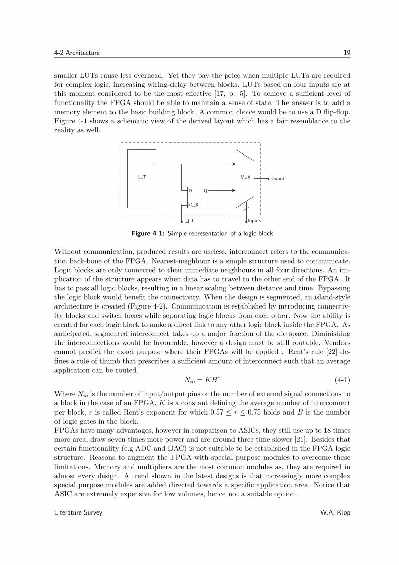
4-2 Architecture 19
smaller LUTs cause less overhead. Yet they pay the price when multiple LUTs are requiredfor complex logic, increasing wiring-delay between blocks. LUTs based on four inputs are atthis moment considered to be the most effective [17, p. 5]. To achieve a sufficient level offunctionality the FPGA should be able to maintain a sense of state. The answer is to add amemory element to the basic building block. A common choice would be to use a D flip-flop.Figure 4-1 shows a schematic view of the derived layout which has a fair resemblance to thereality as well.
LUT
D Q
CLK
Inputs
OuputMUX
Figure 4-1: Simple representation of a logic block
Without communication, produced results are useless, interconnect refers to the communica-tion back-bone of the FPGA. Nearest-neighbour is a simple structure used to communicate.Logic blocks are only connected to their immediate neighbours in all four directions. An im-plication of the structure appears when data has to travel to the other end of the FPGA. Ithas to pass all logic blocks, resulting in a linear scaling between distance and time. Bypassingthe logic block would benefit the connectivity. When the design is segmented, an island-stylearchitecture is created (Figure 4-2). Communication is established by introducing connectiv-ity blocks and switch boxes while separating logic blocks from each other. Now the ability iscreated for each logic block to make a direct link to any other logic block inside the FPGA. Asanticipated, segmented interconnect takes up a major fraction of the die space. Diminishingthe interconnections would be favourable, however a design must be still routable. Vendorscannot predict the exact purpose where their FPGAs will be applied . Rent’s rule [22] de-fines a rule of thumb that prescribes a sufficient amount of interconnect such that an averageapplication can be routed.
Nio = KBr (4-1)
Where Nio is the number of input/output pins or the number of external signal connections toa block in the case of an FPGA, K is a constant defining the average number of interconnectper block, r is called Rent’s exponent for which 0.57 ≤ r ≤ 0.75 holds and B is the numberof logic gates in the block.FPGAs have many advantages, however in comparison to ASICs, they still use up to 18 timesmore area, draw seven times more power and are around three time slower [21]. Besides thatcertain functionality (e.g ADC and DAC) is not suitable to be established in the FPGA logicstructure. Reasons to augment the FPGA with special purpose modules to overcome theselimitations. Memory and multipliers are the most common modules as, they are required inalmost every design. A trend shown in the latest designs is that increasingly more complexspecial purpose modules are added directed towards a specific application area. Notice thatASIC are extremely expensive for low volumes, hence not a suitable option.
Literature Survey W.A. Klop

20 Reconfigurable Computing
Switchbox
Logicblock CB
CB
Switchbox
Logicblock CB
CB
Switchbox
Logicblock CB
CB
Switchbox
Logicblock CB
CB
Switchbox
Logicblock CB
CB
Switchbox
Logicblock CB
CB
Switchbox
Logicblock CB
CB
Switchbox
Logicblock CB
CB
Switchbox
Logicblock CB
CB
Switchbox
Logicblock CB
CB
Switchbox
Logicblock CB
CB
Switchbox
Logicblock CB
CB
Switchbox
Logicblock CB
CB
Switchbox
Logicblock CB
CB
Switchbox
Logicblock CB
CB
Switchbox
Logicblock CB
CB
Blo
ck M
em
ory
Blo
ck M
em
ory
Additional Hardware
Additional Hardware
Figure 4-2: Architecture of FPGA
4-3 Applicability
The fine grained architecture allows virtually any application that can be transformed toBoolean equations to fit in the FPGA structure. Programming or describing, as it is actuallycalled is usually accomplished via a hardware description language (HDL). Such a languageis reasonably low level. Compared to a processor language the level is equivalent to assemblyor even lower. The reconfigurability is associated with flexibility, however the rather com-prehensive describing model suggests the opposite. Regarding these aspects, the technologyplaces itself, with respect to flexibility, between software and hardware category.FPGAs do not confine themselves to a specific domain. The technology benefits largely, if theapplication under consideration, can be mapped to a parallel version. However, FPGAs cancope with sequential sections as well. By producing special purpose modules, the specialisa-tion factor affects the speed-up in a positive manner resulting in a faster version as could beachieved on a general purpose microprocessor. The sequential approach still allows for spatialimplementations by running different special purpose modules simultaneous. The versatilecharacter of the FPGA reduces the number of constraints imposed on the algorithm.Almost any scientific application or algorithm uses matrix multiplications. The elementarybuilding block of a matrix multiplication is a multiply-add operation. The question is howwell suited is an FPGA to perform such operations also referred to as FLOP. Since the hard-ware multipliers inside modern FPGAs, as denoted above, do not fulfil the 32-bit requirementfor single precision FLOPs let alone for double precision. Manufactures offer intellectual
W.A. Klop Literature Survey

4-3 Applicability 21
property (IP) blocks (comparable to libraries in C) to support a variety of FLOPs. Theseblocks use several multipliers and logic units for a single FLOP unit. Using the IP blockmanual and device datasheets from the vendors [36, 37] we are able to determine the theo-retical floating point performance [2, 32]. Taking the Xilinx Virtex 6 FPGA as an example.Table 4-1 gives us the necessary information about the FPGA, where Table 4-2 presents theproperties of the floating point IP block.
Operation DSP Slices LUTs FFs Maximum Frequency (MHz)
Multiply (SP) 3 110 107 114 429
Add (SP) 2 295 287 337 380
Multiply (DP) 11 357 328 497 429
Add (DP) 3 849 834 960 421
Table 4-2: Resource usage of floating point IP block when implemented in Xilinx Virtex-6 FPGA.Multiply and add operations in both single precision (SP) and double precision (DP) are presented.
Depending on the configuration, the theoretical performance can vary between about 306GFLOP single precision and 121 GFLOP for double precision. Assumed is that a multiplierand an add operation always occur in pairs. Take into account that in these calculations, nospace was reserved for control logic or other functionality. It is also common that the allowedmaximal frequency drops when the size of the design increases. It is attractive to use thesefindings as comparison measure for other devices. Doing this neglects the FPGAs ability ofbeing full application specific, whereas other platforms are directed toward a application area.
4-3-1 Overview
Consequences to the algorithm design which are imposed when using FPGA technology:
• Single precision and double precision floating point operations are not directly supportedand requires IP blocks. For each block substantial resources are utilised, limiting thenumber of operations that can be performed parallel.
• Embedded memory is confined in a FPGA. Embedded memory can be used for e.g.registers. Algorithm designers should considers this limitation. Still there is the pos-sibility to augment a FPGA with memory, however usually global memory is severalfactors slower.
• Depending on the type of function some are more expensive in relation to the availableresources than others. A multiply operation requires more resources in contrast to anadd operation. Efficient implementations involves algorithm design which considers theoperation expense.
• A FPGA allows to for tailor made implementations on a hardware level. Reducingoverhead and incompatibility issues. This property is what makes FPGAs a suitableplatform for a wide variety of applications.
Literature Survey W.A. Klop

22 Reconfigurable Computing
W.A. Klop Literature Survey

Chapter 5
Adaptive Optics Algorithms
A critical performance component of the adaptive optics (AO) system is the control algorithmand for existing AO systems this is a well established field. However till now there was noreal need for computational efficient implementations. This has changed with the increaseof interest in ELT’s. The wave front reconstructor which is an essential part of the controlalgorithm where slopes (sk) are used to estimate wave front phases (φk) based on Eq. (1-6).We have seen in the introduction chapter we need to optimise the wavefront reconstructionprocess, as it contributes significant to the computational efficiency of the control algorithm.Often the choice in algorithm lies in a tradeoff between performance and accuracy. Thereare already several suggestions for algorithms that are optimised and try to get the best outof both worlds, e.g. the FFT solution proposed by Poyneer et al. [31] is relatively efficienthowever it compromises in accuracy. On the other side of the spectrum are the model basedpredictors which are accuracy wise optimal [6, 13]. Recently also a new approach is suggestedby Thiébaut and Tallon [33] which uses fractal iterative method (FRiM) as a augmentation tothe minimum variance method. To make a fair judgement three algorithms have been selectedand analysed for their performance and accuracy. The chosen algorithms are expected to bespread throughout the performance versus accuracy spectrum. Each of the algorithms arediscussed in a separate section, partitioned by three subsections. The subsection General Infodescribes the basis and the origin of the algorithm. In Algorithmic Structure, a summaryis given on the operation of the algorithm. Finally an analyse considering the accuracy,performance and suitability for parallel implementation is described.
5-1 Fast Fourier transform reconstruction
5-1-1 General Info
Freischlad and Koliopoulus suggested to use Fourier transformations as a wavefront recon-struction method [14]. In Poyneer et al. [31] the authors investigate and demonstrate thefeasibility of the method for AO systems with at least 10.000 actuators. The motivation
Literature Survey W.A. Klop
24 Adaptive Optics Algorithms
behind using Fourier transformations is that certain operations are easier to perform in thefrequency domain. In contrary stands the fact that now two transformations has to be per-formed. First from the time to the frequency domain and later back again. The use of Fouriertransforms appears to have a second drawback, they are mainly designed to be fast and neverproven to be optimal. subsequent the accuracy has to be verified to be sufficient for thespecific application. Research performed by the authors of [24] and [25] show the results ofexperiments carried out on respectively a Virtex 4 FPGA and a Ge-Force 7800 GTX GPU.They claim that the suggested method of L.A. Poyneer can be solved on both platforms.When a problem size of 256x256 is considered, the FPGA needs around 2.0 ms to come to asolutions and for the GPU it takes 5.2 ms.
5-1-2 Algorithmic Structure
The method is primarily depending on the inverse spatial filter, complementary operations,like the Fourier transform, are obligated to allow the filter to be applied. Furthermore, tomake the method applicable to a AO system of a telescope some pre-processing and post-processing steps has to be undertaken. In Figure 5-1 the complete structure of the algorithmis depicted. As the algorithm is specialised towards an specific sensor geometry each changein this geometry has effect on the algorithm. In the paper the Fried geometry is taken asfoundation and some additional aspects of the Hudgin geometry are elucidated (in the figureshown with dotted lines).
Extend Gradients
Discrete Fourier Transform
Filter
Inverse Discrete Fourier Transform
Modal Removal
Linear Transform
Recombine
ф[m,n]
ф[m,n]
Ф[k,l]
Ф[k,l]
ф[m,n]
ф[m,n]
^
^
^
Figure 5-1: Structure FFT algorithm. Both the process steps of the Fried as the Hudgin geometryare depicted. The additional required by the Hudgin geometry are dashed.
The filter works under the assumption that the aperture is square. However in reality theaperture is always circular. To compensate for this Poyneer et al. [31] suggest two methods.The boundary method where the gradients on the edge of the aperture are used to calculate
W.A. Klop Literature Survey

5-1 Fast Fourier transform reconstruction 25
the gradients that cross the edge. This is achieved by setting up a set of equations andsolving the unknowns. The second one is the extension method, this method extends theouter gradient down, up, left and right. The still missing seam gradients are calculated bysetting the row or column to zero. The boundary method as well as the extension methodconsiders only the noiseless case. In reality noise will always be present and this can influencethe suggested methods. E.g. the boundary method should use linear least squares instead toapproximate a solution. The next step is the transformation to the frequency domain. Thestandard Fourier transform and inverse Fourier transform scales as O(N2) while a lower orderwould be desirable. Fast Fourier transform (FFT) methods, like the Cooley-Tukey methoddescribed in [23, p. 44] or the multidimensional approach [23, p. 149] achieves exactly that,but under the assumption that the problem size is a power of 2. The suggested FFT scalesas O(Nlog2N) instead. In the frequency domain it is possible to apply the inverse filter. Thefilter consists out of calculating the gradients by determining the first differences betweenadjacent phase points, denoted by Eq. (1-4). Transformation to the frequency domain leavesus with equations 5-1.
Sx[k, l] = Φ[k, l][exp( j2πkN )− 1] (5-1)
Sx[k, l] = Φ[k, l][exp( j2πlN )− 1] (5-2)
The inverse filter can be deduced by applying linear least squares in the frequency domainEq. (5-3).
Φ[k, l] =
0, k, l = 0
[exp(− j2πkN )− 1]Sx[k, l] + [exp(− j2πl
N )− 1]Sy[k, l]×[4(sin2 πk
N + sin2 πlN )]−1, else
(5-3)
Transforming the result back to the time domain using a inverse Fourier transformation leavesonly the modal removal to be applied. For certain modes it is beneficial to eliminate themfrom the reconstruction. Due to the fact that Fourier transform introduces significant errorsinto the estimates of particular modes, like waffle and piston. The modal removal process isdone separately, however it can be performed efficient as is depicted in the appendix.
5-1-3 Analysis
A good approach when optimising any algorithm is to analyse to which part of the algorithmthe greatest amount off time is devoted. By selecting this part of the algorithm as first can-didate to be redesigned, will probably give you the highest gain. Each time an optimisationiteration is completed the previous described step should be repeated, based on the fact thatthe part of the algorithm selected before does not have to have the longest execution timeanymore. The analysis only considers the FFT and filter process of the method described byL.A. Poyneer as these processes are rather demanding, the remaining steps can be found inthe appendix and shall be discussed briefly.The pseudo-code off the inverse filter process is depicted in Algorithm 4, studying the codereveals a reasonable amount of calculations. As the calculations are in the frequency domain,
Literature Survey W.A. Klop

26 Adaptive Optics Algorithms
the function variables are complex numbers. Consequently each complex addition or sub-traction involves two floating point operation (FLOP)s. Complex multiplications have even amore severe impact with four regular multiplications and two regular additions they requiresix FLOPs. In the filter equations of the form exp( j2πx
N ) are frequently used. These canbe rewritten as cos(2πx
N ) + i.sin(2πxN ) resulting in three computations. From this knowledge
follows that for example line 3 of the algorithm shall require a total of 10 FLOPs. Settingthe overall number, for a single iteration at 49 FLOPs. To make a fair assessment of theseverity of the computation intensive filter step, the order of the filter should be determined.The algorithm contains a nested for-loop were the main loop requires Nx and the nested loopNy iterations. Let’s define N = NxNy, resulting in an order of O(49N) despite the largeconstant it is assumable that the inverse filter step will not behave as bottleneck. Besides theknowledge that Fourier transformations always produce conjugated pairs allowing for simpli-fications in a further stage. Also, a closer observation shows us that the computations arecompletely independent allowing for an easy transformation to a parallel version.
Algorithm 4 FilterFFT (Φ)
1: for k = 0 to Nx do2: for l = 0 to Ny do
3: Sx ← Φ[k, l][exp ( j2πkNx
)− 1]
4: Sy ← Φ[k, l][exp ( j2πlNy
)− 1]5: if k == 0 and l == 0 then6: Φ[k, l]← 07: else8: Φ[k, l]← [[exp (− j2πk
Nx)− 1]Sx + [exp (− j2πl
Ny)− 1]Sy][4 sin2( πk
Nx) + 4 sin2( πl
Ny)]−1
9: end if10: l← l + 111: end for12: k ← k + 113: end for14: return Φ
FFT referrers to a class of computational efficient (discrete) algorithms to perform Fouriertransformations. Algorithm 5 is a deduction of pseudo-code of an FFT known as Cooley-Tukey [23]. The order of the suggested FFT is O(Nlog2N). Still it should be notified thatthere are again several complex computations involved. While O(Nlog2N) is a substantialprogression, large N still requires a vast amount off effort or more important time. Parallelcomputation could resolve this issue if the FFT allows the conversion. Through the existenceof operations that affect multiple indices, it is possible to conduct that data dependencies arepresent. As discussed before GPU technology is far more sensitive to parallel computing issuesthan FPGA technology. Already suggestions as for example by Moreland and Angel [27] aredone to apply FFT on GPU technology. Their performance results are however comparableto a highly optimised CPU FFT.
W.A. Klop Literature Survey
5-2 Sparse minimum variance reconstruction 27
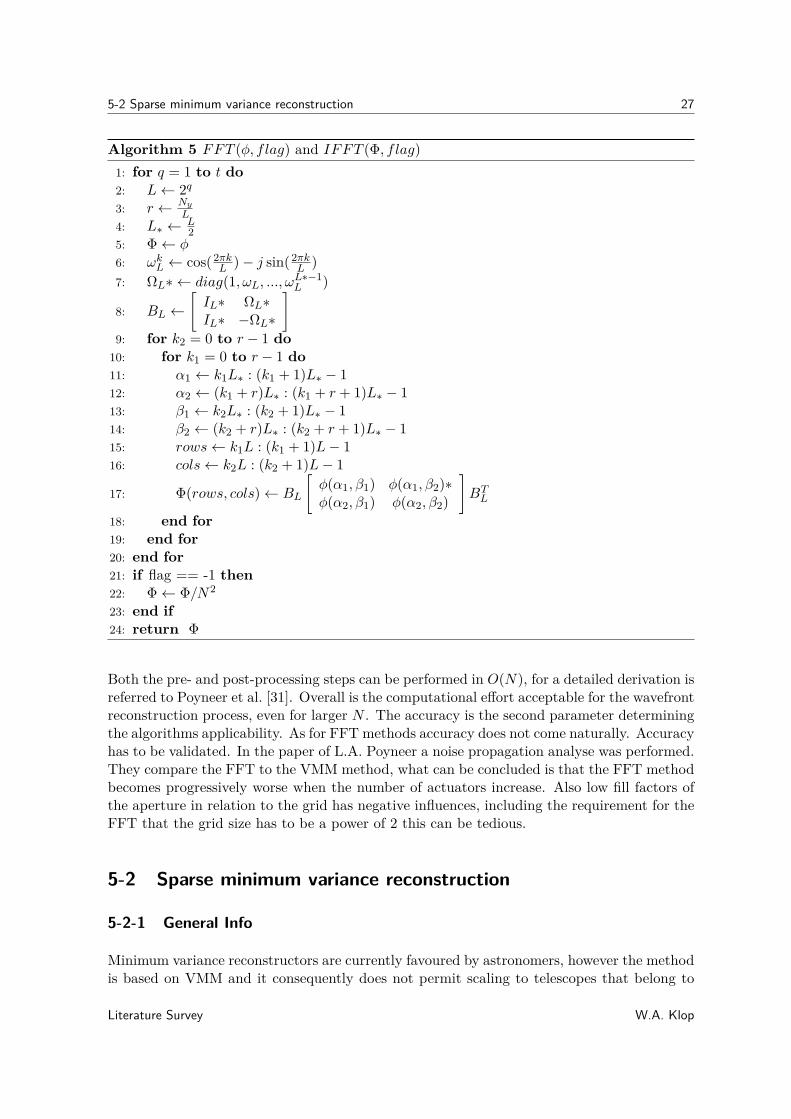
Algorithm 5 FFT (φ, flag) and IFFT (Φ, f lag)
1: for q = 1 to t do2: L← 2q
3: r ← Ny
L4: L∗ ← L
25: Φ← φ6: ωk
L ← cos(2πkL )− j sin(2πk
L )
7: ΩL∗ ← diag(1, ωL, ..., ωL∗−1L )
8: BL ←[
IL∗ ΩL∗IL∗ −ΩL∗
]
9: for k2 = 0 to r − 1 do10: for k1 = 0 to r − 1 do11: α1 ← k1L∗ : (k1 + 1)L∗ − 112: α2 ← (k1 + r)L∗ : (k1 + r + 1)L∗ − 113: β1 ← k2L∗ : (k2 + 1)L∗ − 114: β2 ← (k2 + r)L∗ : (k2 + r + 1)L∗ − 115: rows← k1L : (k1 + 1)L− 116: cols← k2L : (k2 + 1)L− 1
17: Φ(rows, cols)← BL
[
φ(α1, β1) φ(α1, β2)∗φ(α2, β1) φ(α2, β2)
]
BTL
18: end for19: end for20: end for21: if flag == -1 then22: Φ← Φ/N2
23: end if24: return Φ
Both the pre- and post-processing steps can be performed in O(N), for a detailed derivation isreferred to Poyneer et al. [31]. Overall is the computational effort acceptable for the wavefrontreconstruction process, even for larger N . The accuracy is the second parameter determiningthe algorithms applicability. As for FFT methods accuracy does not come naturally. Accuracyhas to be validated. In the paper of L.A. Poyneer a noise propagation analyse was performed.They compare the FFT to the VMM method, what can be concluded is that the FFT methodbecomes progressively worse when the number of actuators increase. Also low fill factors ofthe aperture in relation to the grid has negative influences, including the requirement for theFFT that the grid size has to be a power of 2 this can be tedious.
5-2 Sparse minimum variance reconstruction
5-2-1 General Info
Minimum variance reconstructors are currently favoured by astronomers, however the methodis based on VMM and it consequently does not permit scaling to telescopes that belong to
Literature Survey W.A. Klop
28 Adaptive Optics Algorithms
the class of ELTs. Brent L. Ellerbroek suggest in his paper [6] that sparse matrix techniquescan be applied to overcome this problem. Sparse technologies cannot directly be applied, thepaper describes how to deal with these difficulties. A few times the suggestion is made to useapproximations. For example the turbulence is modelled based on the Kolmogorov turbulencespectrum, where κ defines the spatial-frequency the suggestion is to approximate κ−11/3 asκ−4. These approximations are affecting the accuracy as is addressed in the paper. The gainachieved in contrast to conventional matrix inversion methods is substantial, when consideringa system consisting out of 40,000 actuators, the FLOPs required for the computation ofsparse minimum variance versus conventional matrix inversions is respectively 108 and 1014.5
operations.
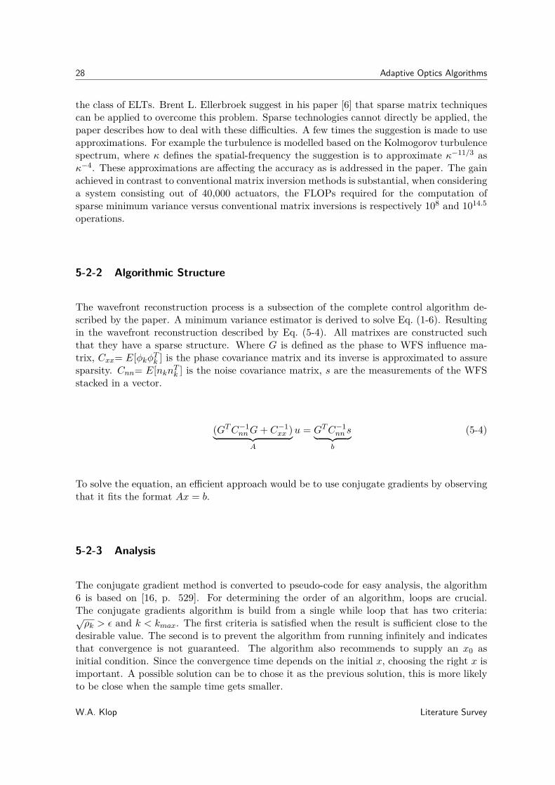
5-2-2 Algorithmic Structure
The wavefront reconstruction process is a subsection of the complete control algorithm de-scribed by the paper. A minimum variance estimator is derived to solve Eq. (1-6). Resultingin the wavefront reconstruction described by Eq. (5-4). All matrixes are constructed suchthat they have a sparse structure. Where G is defined as the phase to WFS influence ma-trix, Cxx= E[φkφT
k ] is the phase covariance matrix and its inverse is approximated to assuresparsity. Cnn= E[nknT
k ] is the noise covariance matrix, s are the measurements of the WFSstacked in a vector.
(GT C−1nn G + C−1
xx )︸ ︷︷ ︸
A
u = GT C−1nn s
︸ ︷︷ ︸
b
(5-4)
To solve the equation, an efficient approach would be to use conjugate gradients by observingthat it fits the format Ax = b.
5-2-3 Analysis
The conjugate gradient method is converted to pseudo-code for easy analysis, the algorithm6 is based on [16, p. 529]. For determining the order of an algorithm, loops are crucial.The conjugate gradients algorithm is build from a single while loop that has two criteria:√
ρk > ε and k < kmax. The first criteria is satisfied when the result is sufficient close to thedesirable value. The second is to prevent the algorithm from running infinitely and indicatesthat convergence is not guaranteed. The algorithm also recommends to supply an x0 asinitial condition. Since the convergence time depends on the initial x, choosing the right x isimportant. A possible solution can be to chose it as the previous solution, this is more likelyto be close when the sample time gets smaller.
W.A. Klop Literature Survey

5-2 Sparse minimum variance reconstruction 29
Algorithm 6 ConjugateGradientsMV (A, b, x0)
1: k ← 12: r ← b−Ax0
3: p← r4: ρ0 ← ‖r‖225: while
√ρk > ε and k < kmax do
6: w ← Ap7: αk ← ρk−1
pT w8: x← x + αkp9: r ← r − αkw
10: βk ← ρk−1ρk−2
11: p← r + βkp12: ρk ← ‖r‖2213: end while14: return x
Inside the loop several computations are carried out, among them is a sparse matrix vectormultiplication. An example algorithm to perform sparse matrix multiplications can be foundin the appendix. With sparse matrix computation technologies, the effort depends also on afill factor denote as f . The fill factor is the percentage of nonzero elements in the matrix. Thefill factor does however not affect the order of a matrix computations, the order of a sparsematrix vector multiplication can be expressed as O(2fN2). Table 5-1 shows that summingthe effort required (5-1) and using the knowledge that the loop is executed maximal kmax
times, leaves us with O(kmax(2 + 10N + 2fN2)) or simplified O(kmaxN2).
Line Number Description Computations Order
6 matrix*vector (Sparse) 2fN2
7 vector*vector and scalar divide 1 + 2N
8 scalar*vector and vector+vector 2N
9 scalar*vector and vector-vector 2N
10 scalar/scalar 1
11 scalar*vector and vector+vector 2N
12 vector*vector 2N
Total 2 + 10N + 2fN2
Table 5-1: Analysis of the conjugate gradient algorithm
When evaluating the order of an algorithm the upper bound is always used as measurement.Directly revealing a bottleneck of the method. Depending on the circumstances the compu-tation can take up to O(kmaxN2), however generally speaking it will perform much betterthrough the sparse matrix computations and due to the fact that kmax will not be reached.In a control loop the worse-case has to serve as leading choice for the control frequency sothis property will be a major disadvantage unless there exists the ability to prove that in thisspecific application the worst-case does not exist. Applying parallel computing to conjugategradient, is due to its dependency on results of previous iterations difficult. In the paperby Bolz et al. [4] a application of conjugate gradients on a GPU is described. To avoid the
Literature Survey W.A. Klop

30 Adaptive Optics Algorithms
data dependencies the auteur’s used a fine grained approach. Consequently the performancelimit is finally determined by the bandwidth of the GPU. As already denoted is the accuracyinfluenced by the approximations. The residual mean squared error is a measure related toaccuracy which was used. In the evaluations Brent L. Ellerbroek has performed there are nosignificant deviations. It should however be denoted that he did not compare the conventionalmatrix inversion with the sparse minimum variance method for larger AO grid sizes.
5-3 Structured Kalman reconstruction
5-3-1 General Info
Rudolf E. Kalman developed a numerical method to estimate true values based on measure-ments corrupted by noise, referred to as the Kalman filter. A dynamical model describingthe behaviour of the system is the basis of the Kalman filter. Under the assumptions thatthe model is linear and the measurements are corrupted by white noise, the Kalman filtercan make an optimal prediction. In the paper by Fraanje et al. [13] the suggestion is to use astructured Kalman filter for the wavefront reconstruction process. To accomplish a structuretheir work is based on a frozen flow turbulence model. By the introduction of sequentiallysemi separable (SSS) matrices it is allowed to use the property that a multiplication withan arbitrary vector can be formatted in a series off subsystems. The gain in structuring theKalman filter is the reduction of complexity at the cost of a slight loss in accuracy.
5-3-2 Algorithmic Structure
A dynamic model always stands at the bases of the Kalman filter. Consequently this approachrequires that together with calculating the Kalman gain a model has to be determined. To cal-culate the kalman gain a computational heavy Ricatti equation has to be solved. Fortunatelythe update rate for the model is presumably rather slow, such that it can be performed offline.Placing the emphasis on the estimation and prediction of the wavefront phases (Figure 5-2).
Determine Model
Solve DARE Equation
Determine Kalman Gain
y(k)
A, C, G
P, S, R
K
Determine Input
Calculate State
Calculate output
y(k)
e(k)
ф(k+1|k)
_
_
_ _
_ _ _
_y
ξ(k+1|k)
^
^
^
Figure 5-2: Wavefront reconstruction algorithm
W.A. Klop Literature Survey

5-3 Structured Kalman reconstruction 31
Depending on the delay between the reading of the sensor and the control of the deformablemirror (DM), it is advantageous to predict several steps ahead. Given the disturbance modelEq. (1-2) and the measurements Eq. (1-6) a predictor can be deduced. Equations 5-5 - 5-7describe a one-step ahead predictor.
e(k) = y(k)− Cy ξ(k|k − 1) (5-5)
ξ(k + 1|k) = Aξ(k|k − 1) + Ky e(k) (5-6)
φ(k + 1|k) = Cξ(k + 1|k) (5-7)
As we are dealing with SSS matrices, equation (5-8) can be applied to compute for exampleu(k) = Ky e(k)
vmi+1(k)
vpi−1(k)ui(k)
=
Kmmi 0 Kme
i
0 Kppi Kpe
i
Kumi Kup
i Kuei
vmi (k)
vpi (k)
ei(k)
, i = 1, ..., N (5-8)
Hence it is possible to reconfigure the equation to form a series of subsystems as is depictedin Figure 5-3. The suggested structure is suitable for an distributed implementation.
Σ1
u1
y1
vm2
vp1
vm1=0
vp0 Σ2
u2
y2
vm3
vp2 ΣN
uN
yN
vmN+1
vpN=0
vmN
vpN-1
Figure 5-3: SSS matrix-vector multiplication as a series of subsystems
5-3-3 Analysis
Matrix vector multiplications utilising the matrices A and C can be implemented efficient byobserving the block structure. Deducing the fact that it is sufficient to determine the matrixvector multiplication result of the block matrices containing information about the innovationmodel simplifies the computation. The remaining blocks are either filled by identity matricesor zeros, resulting in a simple projection of the vector. If Nm defines the order of the innovationmodel the complexity of Aξ(k|k − 1) and equation 5-7 are respectively 2N2
m and 2NyNm.Assume that the WFS resolution corresponds to the grid size and the maximal values for nm
and np are defined as Ny/2. For equations 5-5 and 5-6 the complexity is then respectively4NmNy and 6NNy +6NNm +2N2
m. 6NNy and 6NNm determine the order, Both Nm and Ny
are assumed to be at most N1/2. Leaving us with an order of O(12N3/2). Algorithm 7 showshow a SSS matrix multiplications can be implemented in a sequential fashion. Despite thedistributed design there are dependencies, the intermediate values vm and vp are depended ona previous subsystem. So the system can be distributed but each subsystem has to wait till itsneighbour supplies him with the variable values. The dependency prevents a straightforward
Literature Survey W.A. Klop

32 Adaptive Optics Algorithms
mapping to a parallel version. Note that the matrix vector multiplications related to A andC can be parallelized on a fine grained level like any other standard matrix multiplication.
Algorithm 7 MultiplySSS(A, y(k))
1: n← Size(vm(k))2: vm
0 (k)← 03: vp
n(k)← 04: for i = 0 to n do5: vm
i+1(k)← Ammi vm
i (k) + Amei yi(k)
6: vpn−i−1(k)← App
n−ivpn−i(k) + Ape
n−iyn−i(k)7: i← i + 18: end for
9: n← Rows(A)10: for j = 0 to n do11: ui(k)← Aum
i vmi (k) + Aup
i vpi (k) + Aue
i yi(k)12: j ← j + 113: end for14: return u(k)
The Kalman filter is optimal for systems that are both linear and corrupted by Gaussiandistributed noise. As the paper shows the Kalman filter is achieving Strehl ratio’s close toone. During the redesign to achieve the structured matrices some assumptions were made.Despite the assumptions the impact on the accuracy was minimal, only with extremely lowsignal to noise ratio’s there is a significant difference.
5-4 Overview
Table 5-2 gives an overview of the three algorithms and their suitability with respect to theELT application, order, FPGA implementation and GPU implementation. For the ELT cate-gory the judgement criteria were the performance and accuracy. E.g. the FFT method scoredunsatisfactory on accuracy which explains the "- -". The order is only based on the expectedworst-case scenario hence the poor score for the sparse minimum variance method. The cat-egories FPGA and GPU implementation considers aspects like risk, demonstrated feasibility,(expected) performance and implementation effort. Hardware trends are not included in thescore so only based on current technology. The GPU scores low on each algorithm, which ismainly caused by the lack on coarse grained parallelism in the algorithms. An aspect whereGPUs are highly dependent on.
W.A. Klop Literature Survey

5-4 Overview 33
Algorithm ELT Order FPGA GPU
FFT reconstructor - - - ++ -
sparse MV reconstructor -/+ - - + -
Structured Kalman reconstructor -/+ ++ + -
Table 5-2: An overview of the suitability wit respect to the categories; ELT, Order, FPGA andGPU.
Literature Survey W.A. Klop

34 Adaptive Optics Algorithms
W.A. Klop Literature Survey

Chapter 6
Findings
The objective off the research was to discover the issues that play a role in resolving thethesis; which algorithm in combination with an implementation technology would be suitablefor solving the adaptive optics (AO) related problem of reconstructing the wavefront. Suchthat kilohertz (real-time) performance is feasible? All with respect to the development ofextremely large telescope (ELT)s. To achieve these requirements the focus must lie on thescalability of the design such that it allows for at least 40.000 actuators. During the researchseveral different technologies at different levels are examined on suitability. The technologiescould be classified into two categories algorithms and hardware. In the class algorithms,three methods were addressed: fast Fourier transform (FFT), sparse minimum variance byconjugate gradients and a structured Kalman filter. For the hardware category, graphicsprocessing unit (GPU)s and field programmable gate array (FPGA)s were considered. Avital discovery is that due to the requirements each technology encompasses, there are strongdependencies between the lower level hardware and higher level algorithm.
6-1 Conclusions
Parallel computing is already an essential technology for solving large scale scientific problems.In the future the application segment will evolve to an even wider scope. The majority ofCPU manufacturers already altered their direction towards parallel computing, driven byphysical limitations related to frequency scaling. Parallel computing is therefore a technologyexceptionally suitable to satisfy the real-time requirements related to large scale wavefrontreconstruction of AO systems.GPUs and FPGAs are hardware platforms which support parallel computing. Both paralleldevices are capable to cope with such a task. Each of the platforms have their advantages anddisadvantages, e.g. where the FPGA is a safer choice in the sense that it is more developed,the GPU is more interesting for its potential. The properties of both technologies have theirrequirements on the application implementation. As a consequence the preference off thehardware technology depends primarily on the selected algorithm.
Literature Survey W.A. Klop

36 Findings
Concerning the algorithms, the method suggested by Poyneer et al. [31], using FFT is aboveall fast, while the accuracy is coming on the second place. Especially when larger grid sizesare considered the accuracy issue is playing a significant role, reducing the likelihood thatthe method can be suitable for ELT applications. In contrast the sparse minimum variancemethod designed by Ellerbroek [6] is accurate. However, despite the fact that the generalcase is probably significantly smaller, the worst case is in the order of O(N2). Augmentingthe data dependency issue related to the conjugate gradient method makes this also a nonideal candidate. The sequentially semi separable (SSS) Kalman method suggested by Fraanjeet al. [13] achieves decent results on both performance and accuracy. Hence, it could be asuitable method. When reflecting the algorithm on parallel computing aspects there arises anissue, the interconnection structure imposes several data dependencies introducing sequentialbehaviour. Also it only allows for a fine-grained parallelization approach. Making the FPGAthe technology were the greatest benefit can be achieved. Still implementing this algorithmin FPGA technology is merely a patch than a optimal solution. To use parallel computingto its full extend, the algorithm should rather be adapted or an alternative algorithm shouldbe considered. For example, if it would be possible to introduce delays in the communicationchannels between subsystems, parallelism would improve significantly.
6-2 Recommendations
In the analysis of the algorithms, possible bottlenecks were indicated in relation to parallelcomputing. However a more in-depth study can decide whether there exists a parallel solutionfor the used algorithms or it should be developed. Emphasising on optimality should be vitalhere, due to the fact that when an algorithm merely uses a subset of the available resourcesit will not be sufficient for the AO application under consideration. The suggested researchis necessary to allow future successful implementations on devices like FPGAs and GPUs.An alternative option would be to adopt another approach. The recent suggested algorithmstake existing methods as staring point, to tackle the problem globally. Mapping methods areused to transform the sequential algorithms to the parallel computing domain, often resultingin dependency issues. To avoid dependencies a bottom-up approach could be helpful. Firstdefining the requirement that the algorithm should at least be fully parallel. The methodsuggested by Rufus Fraanje utilises neighbour data under the assumption of frozen flow tur-bulence. Perhaps this is an indication that information of nearest-neighbours is sufficient topredict phase differences provided that the sampling frequency is adequate. An approachis suggested that when achievable could result in a distributed system with only very localdependencies. The approach works under the assumption that each segment can be seenas a loosely coupled system. Starting with developing a local dynamical model where theinputs are the WFS values of the nearest-neighbours and the output the phase difference ofthe segment under consideration. Subsequently by applying Kalman filtering the predictionof the phase difference on a single grid point is estimated. This process is performed foreach segment in parallel completing the wavefront reconstruction. The computational effortto solve a local problem is expected to be low due to the minor size. Generating an addi-tional advantage that the order of the problem will never exceed O(N), allowing for maximalscalability.
W.A. Klop Literature Survey

6-3 Project Proposal 37
6-3 Project Proposal
Since the parallel computing concepts imposes strong requirements on the algorithm it issensible to take these requirements as starting point to attain a successful implementation.For the graduation project I would propose to start a study to a nearest-neighbour approachsuggested in the recommendations section. Hence the thesis will become: Is it possible todesign and implement a fully parallel wavefront reconstruction algorithm solely based onnearest neighbour information? To answer the thesis a phased approach is suggested asdepicted in Figure 6-1.
Algorithm design
Experiments in Matlab
Satisfactory
results
Implementation FPGA/GPU
Simulations
Su!cient
Time
Finishing thesis report
no
no
yes
yes (optimize)
No
ve
mb
er
De
cem
be
r
Jan
ua
ryFe
bru
ary
Ma
rch / A
pril
Ma
yW
riti
ng
re
po
rt
Figure 6-1: Graduation project proposal
As the suitability of hardware technology hugely depends on the algorithm structure choosingthe hardware platform is still a open question. Since time is limited the most suitable platformwill be implemented considering the developed algorithm.
Literature Survey W.A. Klop

38 Findings
W.A. Klop Literature Survey
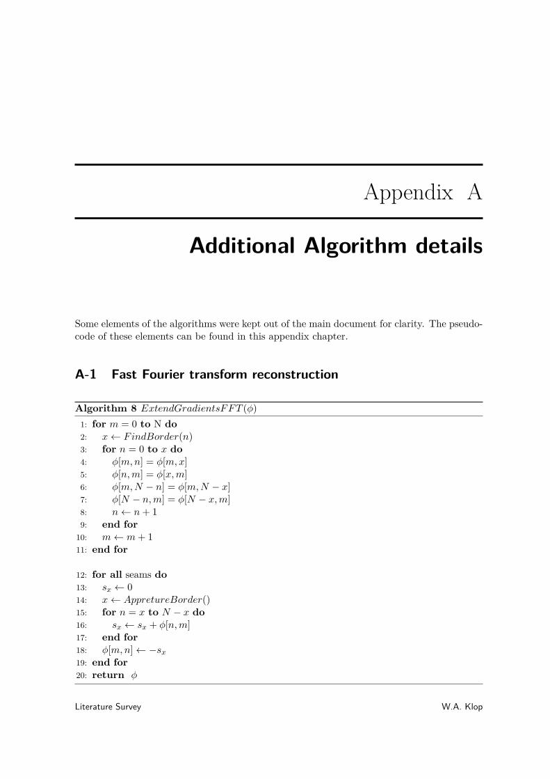
Appendix A
Additional Algorithm details
Some elements of the algorithms were kept out of the main document for clarity. The pseudo-code of these elements can be found in this appendix chapter.
A-1 Fast Fourier transform reconstruction
Algorithm 8 ExtendGradientsFFT (φ)
1: for m = 0 to N do2: x← FindBorder(n)3: for n = 0 to x do4: φ[m, n] = φ[m, x]5: φ[n, m] = φ[x, m]6: φ[m, N − n] = φ[m, N − x]7: φ[N − n, m] = φ[N − x, m]8: n← n + 19: end for
10: m← m + 111: end for
12: for all seams do13: sx ← 014: x← AppretureBorder()15: for n = x to N − x do16: sx ← sx + φ[n, m]17: end for18: φ[m, n]← −sx
19: end for20: return φ
Literature Survey W.A. Klop

40 Additional Algorithm details
Algorithm 9 ModalRemovalFFT (φ)
1:∑
φv ← 02:
∑
vv ← 03: for m = 0 to N do4: for n = 0 to N do5:
∑
φv ←∑
φv + ˆphi[m, n]v[m, n]6:
∑
vv ←∑
vv +v[m, n]v[m, n]7: n← n + 18: end for9: m← m + 1
10: end for
11: cv ←∑
φv∑
vv
12: for m = 0 to N do13: for n = 0 to N do14: φfinal[m, n]← φ[m, n]− cvv[m, n]15: n← n + 116: end for17: m← m + 118: end for19: return φfinal
W.A. Klop Literature Survey

A-2 Sparse minimum variance reconstruction 41
A-2 Sparse minimum variance reconstruction
Algorithm 10 SparseMatrixMulMV (A, B)
1: for i = 0 to NumberOfRows(A) do2: for j = 0 to NumberOfColumns(B) do3: rowi ← A.GetRow(i)4: colj ← B.GetCol(j)5: sum← 0
6: while not rowi.IsEmpty() and not colj .IsEmpty() do7: if rowi.item.index == colj .item.index then8: sum← sum + row.item.value ∗ col.item.value9: rowi.item.GetNext()
10: colj .item.GetNext()11: else if rowi.item.index < colj .item.index then12: rowi.item.GetNext()13: else14: colj .item.GetNext()15: end if16: C[i, j]← sum17: end while18: j ← j + 119: end for20: i← i + 121: end for22: return C
A-3 Structured Kalman reconstruction
Algorithm 11 V ectorAdition(z(k), y(k))
1: n← Size(z(k))2: for i = 0 to n do3: u(k)← zi(k) + yi(k)4: i← i + 15: end for6: return u(k)
Literature Survey W.A. Klop

42 Additional Algorithm details
W.A. Klop Literature Survey

Bibliography
[1] Advanced Micro Devices, Inc. AMD FireStreamT M 9270 GPU Compute Accelerator .www.amd.com/stream, May 2010.
[2] Altera Corporation. White paper - designing and using fpgas for double-precisionfloating-point math. www.altera.com/literature/wp/wp-01028.pdf, August 2007.
[3] Altera Corporation. Stratix v device family overview.www.altera.com/literature/hb/stratix-v/stx5_51001.pdf, July 2010.
[4] Jeff Bolz, Ian Farmer, Eitan Grinspun, and Peter Schroder. Sparse matrix solvers on theGPU: Conjugate gradients and multigrid. ACM transactions on graphics, 22, 2003.
[5] Frederick P. Brooks. The mythical man-month. Addison Wesley Publishing, 1995.
[6] Brent L. Ellerbroek. Efficient computation of minimum-variance wave-front reconstruc-tors with sparse matrix techniques. Optical Society of America, 19(9), September 2002.
[7] Gerald Estrin, editor. Organization of Computer Systems - The Fixed Plus Variable
Structure Computer, New York, 1960. Western Joint Computer Conference, Proc. West-ern Joint Computer Conf.
[8] Gerald Estrin. Reconfigurable computer origins: the ucla fixed-plus-variable (f+v) struc-ture computer. IEEE Annals of the History of Computing, 24(4), October 2002.
[9] Kayvon Fatahalian and Mike Houston. A closer look at GPUs. communications of the
acm, 51(10), oktober 2008.
[10] Kayvon Fatahalian and Mike Houston. NVIDIA tesla: a unified graphics and computingarchitecture. Hot Chips, April 2008.
[11] Enrico Fedrigo and Robert Donaldson. Sparta roadmap and future challenges. Adaptive
Optics Systems II, 7736(1):77364O, 2010.
[12] Michael J. Flynn. Some computer organizations and their effectiveness. IEEE Transac-
tions on computers, 1972.
Literature Survey W.A. Klop

44 BIBLIOGRAPHY
[13] Rufus Fraanje, Justin Rice, Michel Verhaegen, and Niek Doelman. Fast reconstructionand prediction of frozen flow turbulence based on structured kalman filtering. Optical
Society of America, 2010.
[14] Klaus R. Freischlad and Chris L. Koliopoulos. Modal estimation of a wave front fromdifference measurements using the discrete fourier transform. Optical Society of America
A, 3(11), November 1986.
[15] Gene Golub and James M. Ortega. Scientific Computing An Introduction with Parallel
Computing. Academic Press inc, London, United Kingdom, 1993.
[16] Gene H. Golub and Charles F. van Loan. Matrix Computations. The Johns HopkinsUniversity Press, Baltimore, Maryland, 1996.
[17] Scott Hauck and Andre DeHon. Reconfigurable Computing. Morgan Kaufmann Publish-ers, Burlington, 2008.
[18] John L. Hennessy and David A. Patterson. Computer Architecture; A Quantitative
Approach. Morgan Kaufmann, 4th edition, 2007.
[19] G.J. Hovey, R. Conan, F. Gamache, G. Herriot, Z. Ljusic, D. Quinn, M. Smith, J.P.Veran, and H. Zhang. An fpga based computing platform for adaptive optics control. 1st
AO4ELT conference, 2010.
[20] David Kirk and Wei-Mei Hwu. Programming Massively Parallel Processors. ElsevierScience and Technology, 2010.
[21] Ian Kuon and Jonathan Rose. Measuring the Gap between FPGAs and ASICs. FPGA,06, February 2006.
[22] Bernard S. Landman and Roy L. Russo. On a Pin Versus Block Relationship For Parti-tions of Logic Graphs. IEEE transactions on computers, c-20(12), December 1971.
[23] Charles Van Loan. Computational Frameworks for the Fast Fourier Transform. SIAM,Philadelphia, 1992.
[24] Eduardo Magdaleno, Manuel Rodríguez, José Manuel Rodríguez-Ramos, and Alejan-dro Ayala. Modal fourier wavefront reconstruction using fpga technology. Micro and
Nanosystems, 1(1), 2009.
[25] José G. Marichal-Hernández, José M. Rodríguez-Ramos, and Fernando Rosa. Modalfourier wavefront reconstruction using graphics processing units. Journal of Electronic
Imaging, 16(2), June 2007.
[26] Gordon E. Moore. Cramming more components onto integrated circuits. Electronics,1965.
[27] Kenneth Moreland and Edward Angel. The FFT on a GPU. Graphics Hardware, 2003.
[28] NVIDIA Corporation. NVIDIA Tesla C2050/C2070 Datasheet. www.nvidia.com/tesla,July 2010.
W.A. Klop Literature Survey

BIBLIOGRAPHY 45
[29] John D. Owens, David Luebke, Naga Govindaraju, Mark Harris, Jens Krüger, Aaron E.Lefohn, and Timothy J. Purcell. A survey of general-purpose computation on graphicshardware. Computer Graphics forum, 26(1), 2007.
[30] John D. Owens, Mike Houston, David Luebke, Simon Green, John E. Stone, and James C.Phillips. GPU Computing. Proceedings of the IEEE, 96(5), May 2008.
[31] Lisa A. Poyneer, Donald T. Gavel, and James M. Brase. Fast wave-front reconstructionin large adaptive optics systems with use of the fourier transform. Optical Society of
America, 19(10), October 2002.
[32] Dave Strenski. Fpga floating-point performance - a paper and pencil evaluation.www.hpcwire.com/hpc/1195762.html, January 2007.
[33] Eric Thiébaut and Michel Tallon. Fast minimum variance wavefront reconstruction forextremely large telescopes. Optical Society of America, 25(5), May 2010.
[34] Tuan N. Truong, Antonin H. Bouchez, Richard G. Dekany, Stephen R. Guiwits, Jen-nifer E. Roberts, and Mitchell Troy. Real-time wavefront control for the palm-3000 highorder adaptive optics system. Proceedings of the SPIE, 7015, 2008.
[35] R. N. Wilson. Reflecting Telescope Optics I. Springer-Verlag Berlin Heidelberg, Germany,1996.
[36] Xilinx Inc. Floating-point operator v5.0 - product specification.www.xilinx.com/support/documentation/ip_documentation/floating_point_ds335.pdf,June 2009.
[37] Xilinx Inc. Virtex-6 family overview - advance product specification.www.xilinx.com/support/documentation/data_sheets/ds150.pdf, January 2010.
Literature Survey W.A. Klop

46 BIBLIOGRAPHY
W.A. Klop Literature Survey

Glossary
List of Acronyms
ADC analog-to-digital converter
AO adaptive optics
API application programming interface
ASIC application specific integrated circuits
CPU central processing unit
CUDA Compute Unified Device Architecture
DAC digital-to-analog converter
DSP digital signal processor
DM deformable mirror
E-ELT European extremely large telescope
ELT extremely large telescope
ESO European Southern Observatory
FF flip-flop
FFT fast Fourier transform
FLOP floating point operation
FPGA field programmable gate array
FRiM fractal iterative method
HDL hardware description language
GPGPU general-purpose computing on graphics processing units
Literature Survey W.A. Klop

48 Glossary
GPU graphics processing unit
IC integrated circuit
IP intellectual property
LUT look-up table
MIMD multiple instruction multiple data
OpenCL Open Computing Language
PLD programmable logic devises
PROM programmable read-only memory
SIMD single instruction multiple data
SIMT single instruction multiple thread
SSS sequentially semi separable
VMM vector matrix multiply
WFS wavefront sensor
List of Symbols
α The fraction of code that is not parallelizable
λ Wavelength of the light emitted by the object under observation
φ Phase difference vector
θ Angular resolution
B Number of logic gates in the block
C The capacitance switched per clock cycle
Cnn Noise covariance matrix
Cxx Phase covariance matrix
D The diameter of the aperture
e Gaussian distributed noise
Enew Executing time for entire task using the enhancement when possible
Eold Execution time for entire task without using the enhancement
F The frequency at which the IC is running
G The phase-to-WFS influence matrix
H The DM influence matrix
K Constant defining the average number of interconnect per block
k Time index
W.A. Klop Literature Survey

49
Nio The number of input/output pins or the number of external signal connectionsto a block
p The number of processing units
r Rent’s exponent
Sp Speedup factor related to the run time of the original code
sx[m, n] Measured phase gradients in the x direction
sy[m, n] Measured phase gradients in the y direction
uk Control inputs
V The supply voltage
z−1 Discrete shift operator
Literature Survey W.A. Klop

50 Glossary
W.A. Klop Literature Survey