Discussion Paper No.79 Dec 2008

Liquidity Risk and Bank Portfolio Management in

a Financial System without Deposit Insurance:

Empirical Evidence from Prewar Japan

澤田 充

名古屋学院大学総合研究所

University Research Institute

Nagoya Gakuin University

Nagoya, Aichi, Japan

1

Liquidity Risk and Bank Portfolio Management in a Financial System without Deposit Insurance: Empirical Evidence from

Prewar Japan*

Michiru Sawada

Faculty of Economics, Nagoya Gakuin University, 1-25 Atsutanishi-machi, Atsuta-ku, Nagoya-shi, Aichi 456-8612, Japan

(E-mail address: sawada@ngu.ac.jp)

Abstract

Using data from prewar Japan, this paper investigates the impact of liquidity shock on

bank portfolio management during financial crises in a system lacking deposit

insurance. It is found that banks faced with a rise in their liquidity risk increased their

cash holdings not by liquidating bank loans but by selling securities in the financial

market. Moreover, banks exposed to local financial contagion adjusted the liquidity of

their portfolio mainly by actively selling and buying their securities in the financial

market. Finally, there is no evidence to conclude that the existence of the lender of last

resort mitigated the liquidity constraints in bank portfolio adjustments.

JEL Classification; G21, O16, N25

Keywords; Bank portfolio; Financial contagion; Lender of last resort; Liquidity risk * I would like to thank Professor Kaoru Hosono, Masaki Nakbayashi, Ichihiro Uchida, Nobuyoshi Yamori, and other participants at The Japan Society of Monetary Economics and Business History Society of Japan, for their helpful comments and suggestions. Special thanks also go to Professor Tetsuji Okazaki for approval to use financial data of banks. All errors are the authors’ responsibility.

2

1. Introduction

One of the most important roles of banks is to perform the maturity transformation of

assets by issuing short-term liabilities and holding long-term assets. Therefore, given a

system where depositors are insufficiently protected, banking systems are potentially

exposed to the probability of bank runs. In fact, during prewar periods, bank runs

occurred frequently in the U.S., Europe, Japan, and contemporary emerging countries

where deposit insurance was nonexistent.

Since Diamond and Dybvig (1983), a considerable number of studies have been

conducted on bank runs and panics. The majority of these studies have focused on the

origin and causes of bank runs, which can be classified into two alternative views. The

first is the random withdrawal theory, which considers bank runs as self-fulfilling

phenomena (e.g., Waldo (1985); Postle and Vives (1987); Chang and Velasco (2000,

2001)). The other is the information based theory, which considers bank runs as

phenomena induced by the market discipline of depositors under the asymmetric

information (e.g., Gorton (1985); Chari and Jagannathan (1988); Calomiris and Gorton

(1991)). Recently, there has been renewed interest in portfolio management with respect

to economies where runs are possible (Cooper and Ross (1998); Peck and Shell (2003);

Ennis and Keister (2006); Franck and Krausz (2007)). These studies, developing

Diamond and Dybvig (1983), analyze how banks manage the liquidity of their portfolios

taking into account the strategic behavior of depositors. Cooper and Ross (1998) and

Ennis and Keister (2006) examine the relation between the probability of a bank run

and the level of liquid assets held by banks. Peck and Shell (2003) investigate how

restrictions on the holding of illiquid assets affect the level of liquid assets chosen by

banks. Franck and Krausz (2007) analyze the impact of the stock market and the

presence of a lender of last resort (LLR) on the portfolio allocations of banks when they

are faced with random withdrawals by depositors. Despite such theoretical

3

developments, empirical evidence is lacking on the liquidity management of banks in a

system devoid of deposit insurance—at least, since Friedman and Schwartz (1963).

These authors demonstrated that the deposit-reserve ratio is inclined to decrease

during periods of banking crisis (as in 1907 and the early 1930s). However, they

analyzed the time-series behavior of banks on the basis of aggregate data. Moreover,

they did not conduct a detailed statistical analysis. Therefore, few details are available

on the behavior of individual banks that are exposed to liquidity risk in a system

without deposit insurance.

To investigate portfolio management with respect to banks exposed to liquidity risk,

this study uses micro-level data pertaining to the prewar Japanese banking industry. In

pre-war Japan, since numerous small banks operated without deposit insurance, the

banking sector was subject to liquidity risk due to the frequent occurrence of bank runs.

In fact, nationwide bank runs occurred in the late 1920s and early 1930s, which

resulted in numerous bank closures. This paper focuses on bank behavior during the

banking crisis from 1927 to 1932. —to this author’s knowledge, the first time bank-level

analysis is used to examine the liquidity management of banks operating without

deposit insurance during past periods of financial crises.

This paper examines how banks adjusted the liquidity of their asset portfolios in

response to liquidity shocks during periods of banking crises. Concretely, I focus on a

deposit shock of a bank to capture its liquidity risk, and analyze its effect on the

proportions of three assets in its asset portfolio—loans, cash, and securities. If a bank

fears a future liquidity shortage due to a significant outflow of deposits, then the bank is

expected to increase its proportion of liquid assets such as cash and securities and

decrease its proportion of illiquid assets such as loans. In the very short run, however, it

is difficult to liquidate non-marketable assets such as loans. Thus, this paper also

investigates the impact of contagion on bank portfolios in order to capture the effect of a

4

temporary deposit shock. Furthermore, I examine the influence of the central bank as

the lender of last resort on the portfolio management of private banks. The existence of

the LLR from the central bank is likely to affect the portfolio management of private

banks when the former guarantees the supply of loans to the latter in times of

emergency. In prewar Japan, the Bank of Japan (BOJ), which was the central bank of

Japan, exercised the role of the LLR by providing loans to private banks during periods

of financial crises. Moreover, the BOJ had a well-known tendency to provide LLR loans

to banks with which it had an established transactional relationship (Ishi (1980);

Shiratori (2003); Okazaki (2007)). The role of the LLR is herein further examined

through an analytical comparison of the portfolio management of the BOJ’s

correspondent banks and non-correspondent banks.

This paper is in line with the recent policy discussions on the need to create financial

safety nets. It is generally recognized that deposit insurance suffocates market

discipline, although it is effective in preventing self-fulfilling depositor runs that induce

bank panic. Many financial economists point out the importance of market discipline

and propose various safety net designs to guarantee, among other things, its proper

functioning (Kane (2000); Demirguc-Kunt and Huizinga (2004); Demirguc-Kunt, Kane,

and Laeven (2006)). However, the cost impact on banks that operate without deposit

insurance is not thoroughly understood, particularly in terms of bank behavior1. In light

of these arguments, this paper will attempt to provide useful evidence.

The remainder of this paper is organized as follows. Section 2 discusses the historical

background of the Japanese banking system. Section 3 describes the study’s data and 1 For instance, as stated in Ennis and Keister (2006), a bank that is exposed to the possibility of a bank run might hold more reserves, which leads to a decrease in long-term lending and consequently has an effect on economic activities to some degree.

5

methodology. Section 4 presents the study’s main results. Section 5 considers the impact

of financial contagion on bank portfolios. Section 6 addresses the role of the LLR and

the BOJ. Section 7 concludes the study.

2. A Historical Background

The industrial organization of the prewar Japanese banking sector differed

substantially from its postwar counterpart. An interesting feature is that this industry

was composed of numerous small banks, which was due to the lax regulations that

facilitated entry into the banking industry. Indeed, in the early twentieth century, the

number of banks exceeded two thousand2. However, a safety net for depositors was not

properly established. That is, since deposit insurance was inexistent in prewar Japan, it

was not rare for depositors to incur losses when banks fell into bankruptcy (Takahashi

and Morigaki (1968); Imuta (2001)). Therefore, the banking industry was frequently

susceptible to a series of runs, which resulted in the closure of many banks, particularly

in the 1920s after the collapse of the speculative bubble that followed the economic

boom of the World War I. Table 1 provides historical data related to liquidity shocks in

Japanese banking industry from 1922 to 1935. The number of bank closures is

particularly high during the late 1920s and early 1930s. This period includes major

historic Japanese financial crises namely, the Showa Financial Crisis of 1927 and the

Showa Depression from 1930 to 1931, when nationwide bank runs occurred3. In

addition it is noteworthy that while the growth rate of total deposits of all banks was 2 In 1901, the number of banks reached a peaked at 2334 (1890 ordinary banks and 444 saving banks). Thereafter, the numbers decreased due to the change in government policy. Specifically, in addition to the imposition of strict restrictions on new entrants, the Ministry of Finance promoted bank consolidation efforts. For example, The Bank Law of 1927 obliged an ordinary bank to maintain an amount of capital of not less than one million yen by 1932, and forbade them to increase capital by their own means. Therefore, many banks were forced to choose a merger or a dissolution (Okazaki and Sawada (2007)). 3 For further details on the Showa Financial Crisis and the Showa Depression, see Hoshi and Kashyap (2001, p29-31).

6

negative from 1927 to 1931excepting 1928, the postal savings continued to grow at more

than 10%. These figures are considered to reflect the risk-averse behavior of depositors

during banking crises. As such, Japanese banks suffered from a liquidity crisis,

particularly in the late 1920s and early 1930s.

The BOJ, which was the central bank of Japan, attempted to stabilize the financial

system through its role as the lender of last resort (Ishii (1980); Okazaki (2007)). The

BOJ performed its role as LLR by providing special loans to private banks during a

liquidity crisis. Principally, the special loans helped banks cope with emergencies in the

banking system4. According to Table 1, the share of special loans in the total domestic

loans provided by the BOJ reached 90% in the end of 1920s. Moreover, the amount of

outstanding special loans rose sharply after 1927 when the financial crisis was very

severe.

Another feature of the prewar Japanese banking industry was that many banks

were controlled by industrial companies through capital and personal relationships.

These so-called organ banks generally gave loans to their affiliated industrial group

(Okazaki, Sawada, and Yokoyama (2005)). Therefore, lending was the most important

component among bank assets5. Figure 1 displays the total amount of loans, security

holdings, and cash assets—where cash assets indicate the sum of cash holdings and

deposits with the BOJ and other banks—held by all ordinary banks from 1912 to 1936.

Reflecting the economic boom generated by World War I, the amount of loans was 4 Special loans included loans based on special laws and other loans supplied at the discretion of the BOJ. The special laws refer to the loss in compensation due to the Earthquake Bill Law, the Bill Discount Act passed in 1923, the Bank of Japan Special Loan and Loss Compensation Law passed in 1927, and the Loan to the Taiwan Bank Law passed in 1927 (Okazaki (2007)). 5 The modern history of the Japanese banking industry started with the establishment of national banks in 1872, which were authorized to issue bank notes. The issue of bank notes was accompanied by the requirement to hold the same amount of government bonds according to the National Bank Act. Therefore, the share of government bonds in bank assets was over 60% in 1887. However, this share in 1890 decreased by 20% due to a wave of newly established private banks and the transformation of national banks into private banks.

7

increased substantially in the second half of the 1910s. However, this upward trend was

reversed at the financial turning point of the mid-1920s. Bank loans continued to

decrease from the late 1920s to the early 1930s, when the Japanese economy fell into a

chronic recession after the collapse of the speculative bubble and the impact of the 1923

Great Kanto Earthquake in Tokyo6. By contrast, security holdings principally grew

during these periods—as a result likely due to the imposition on banks to hold liquid

assets, since bank runs frequently occurred during the 1920s and early 1930s (Imuta

(1980); Nanjo and Kasuya (2005)). The structural change in the financial market after

the 1920s additionally affected bank security holdings. While the corporate bond

market was expanding against a background in which bond issuance was aggressively

stimulated by the low interest monetary policies of the second half of the 1920s, the

amount of government bonds underwritten by the Bank of Japan grew rapidly after the

early 1930s due to an increase in fiscal and military expenditures7. According to

Shimura (1969) and Nanjo and Kasuya (2005), a significant amount of funds were

shifted into a number of large banks during various financial crises, and the surplus

funds were thereafter actively invested in securities by the banks. In contrast to loans

and securities, cash assets did not change dramatically after the 1920s. Figure 2

illustrates the proportions of these three assets during this period8. It is noteworthy

that after the mid-1920s, the proportion of securities increased while that of loans

decreased; therefore, security holdings exercised a significant role in the asset portfolios

of banks after the mid-1920s.

Table 2 illustrates the composition of securities holdings in ordinary banks from 1927

to 1935. The share of the sum of all types of bonds reached approximately 90% of total

6 The loss as a result of this earthquake amounted to approximately 5 billion yen, which was equivalent to about 30 % of GNP at that time (Hoshi and Kashyap, (2001)). 7 According to Shimura (1969), 60-80% of government bonds underwritten by the Bank of Japan from 1932 and1936 were sold to private banks. 8 The denominator is the sum of these three assets.

8

security holdings. It is notable that 40–50% of security holdings were government bonds,

which may reflect the need of most banks to reserve liquid assets as insurance against

large withdrawals of deposits (Nanjo and Kasuya (2005)). By contrast, stock shares

were generally low. Shimura (1969) indicates that bank managers hesitated to invest in

stocks because they were considered to be too risky to invest in. .

3. Methodology

In the following analysis, I use panel data from 1926 to 1932 to determine how banks

dealt with liquidity risk through portfolio management. Concretely, I capture a bank’s

liquidity risk by a deposit shock and examine its effect on the liquidity of the asset

portfolio. As mentioned previously, the period of analysis corresponds to a time when

the banking industry was frequently susceptible to a liquidity crisis such as a series of

bank runs. The main data is sourced from the Yearbook of the Bank Bureau issued by

the Ministry of Finance (Ginkokyoku Nenpo), which covers the financial data of all the

banks controlled by the Ministry of Finance9.

Since it was only possible to obtain the sums of all the types of securities held by

banks from the individual financial data available in the Ginkokyoku Nenpo, we

consider both cash assets and security holdings to be liquid assets in the following

analysis. Concerning the degree of liquidity of securities held by banks, it is important

to note how readily or inexpensively the banks could realize these in the financial

market. Government bonds were actively traded after the 1920s because of the reform

of a secondary market that progressed drastically10. On the basis of the historical

records of several banks, Nanjo and Kasuya (2005) stated that banks held government 9This source does not carry all account items. Especially, it is mostly limited to balance-sheet data. 10 Nanjo and Kausya (2005) demonstrated that the ratio of a trading volume at the Tokyo Stock Exchange with respect to the total value of the outstanding amount of issues exceeded 30% in 1928. In addition, government bonds were traded at over-the-counter markets in more than several times the amount of the trading volume at the Tokyo Stock Exchange (Shimura (1969); Bond Underwriters Association of Japan(1980)).

9

bonds as reserve assets because they could be immediately sold in the financial market,

and that such bonds were accepted as collateral when borrowing from the Bank of

Japan. Therefore, government bonds were considered to be highly liquid. The

information on the secondary market of corporate bonds is very limited, since they were

primarily traded in over-the–counter markets (Shimura (1969); Bond Underwriters

Association of Japan(1980)). However, Kasuya (2003) showed the historical records that

large regional banks sold corporate bonds before maturity and bought those

outstanding bonds, and inferred that the secondary market for corporate bonds was

present to some degree.

It was difficult, however, to liquidate bank loans easily because the liquidation

markets were limited11. Moreover, since the loans given by organ banks to related

groups were generally fixed, banks could not always collect the loans at the time of

maturity (Kato (1957)). Therefore, bank loans were considered to be relatively illiquid

as compared to securities and cash assets.

I investigate how banks dealt with liquidity risk through portfolio management. The

basic equations used for this study’s estimations are as follows:

itititit

uXLiqRiskAC

++∆+=⎟⎠⎞

⎜⎝⎛∆ −− 1110 　 γαα (1)

itititit

vXLiqRiskAS

++∆+=⎟⎠⎞

⎜⎝⎛∆ −− 1110 γββ (2)

itititit

wXLiqRiskA

CS++∆+=⎟

⎠⎞

⎜⎝⎛ +

∆ −− 1110 　 γλλ (3)

11 Tsurumi (2001) stated that the interbank markets in prewar Japan included bill discount markets in addition to call loan markets. Therefore, bank loans could be partly liquidated in the financial market. According to Goto (1970, p87) The proportion of discounted bills to total bank loans was approximately 20% in the early 1920s and continued to decline gradually afterward.

10

(Ait = Sit + Cit + Lit)

where S, C, L, and A, are security holdings, cash assets, loans, and total assets,

respectively. Total assets indicate the sum of security holdings, bank loans, and cash

assets12. I use three indices, each as an independent variable, for the liquidity of assets

in a bank portfolio. Moreover, ∆(C/A)it denotes the change in the ratio of cash assets to

total assets (cash-asset ratio) of bank i from year t – 1 to year t. In addition, ∆(S/A)it and

itASC )( +

∆ are the changes in the ratio of securities to total assets (security-asset ratio)

and the ratio of securities plus cash assets to total assets (liquid asset ratio) from year t

– 1 to year t, respectively (hereinafter, we use the term liquid assets to indicate the sum

of securities and cash assets). A positive value in these variables indicates that a bank’s

portfolio has become more liquid. Here, the annual change in the liquid asset ratio

( itASC )( +

∆ ) is equal to the negative value of the annual change in the illiquid asset ratio

(∆(L/A)it), by definition.

In explanatory variables, ∆LiqRiskit–1 indicates a variable for a deposit shock, which

determines the liquidity risk of a bank. We use the deposit growth rate and the annual

change in the deposit-to-loan ratio as ∆LiqRiskit–1, respectively. The deposit-to-loan

ratio is considered to be not only an indicator of the ability to collect deposits but also an

indicator of the liquidity position of a bank, particularly in the field of bank risk

analysis (Van Greuning and Brajovic Bratanovic(2000), among others)14. A negative

value in these variables indicates that the liquidity risk of the bank has become higher.

12 Ginkokyoku Nenpo did not provide the precise figures for total assets in the individual financial data but rather in the aggregate balance-sheet data of all banks. However, the information on the rest of the accounting items of bank assets is not significantly important from the viewpoint of analyzing the portfolio management of banks assets. Moreover, the share of the sum of these three assets (security holdings, cash assets, and loans) to precise total assets exceeded 90%, based on the figures in the aggregate balance-sheet data for 1928. 14 See Van Greuning and Brajovic Bratanovic (2000), Chapter 8.

11

Taking simultaneity into account, deposit shock variables are lagged by one period

based on independent variables. These variables determine the change from year t – 2

to year t – 1. Xit–1 is a vector of other control variables. It includes the natural log of

one-year-lagged total assets and year dummies. In the following analyses, we estimate

these equations from 1928 to 1932 by OLS.

Before the analysis, I will consider the expected effects liquidity shocks on asset

portfolios. If banks fear a future liquidity shortage due to negative deposit shocks, they

are expected to liquidate their bank loans as quickly as possible. Moreover, Cooper and

Ross (1998) (hereinafter, referred to as CR) and Ennis and Keister (2006) (hereinafter,

referred to as EK) treat similar situations in their models. CR (1998)—expanding upon

the work of Diamond and Dybvig (1983)—assume that a bank determines the allocation

of liquid investments in the short term and illiquid investments in the long term,

provided that a run will occur with some fixed probability. Although an illiquid

investment is more productive than a liquid investment, it involves some costs when

liquidated before its maturity. It is demonstrated that banks hold more liquid assets

when bank runs are increasingly probable and the liquation costs of bank investments

are higher. EK (2006) correct and expand upon some results proposed by CR15 EK also

demonstrate that the level of liquid assets held by banks increases with the probability

of a run given a sufficiently high level of liquidation costs16. Generally, banks with high

15 Cooper and Ross (1998) demonstrate that when the probability of a run is small, the bank will offer a contract that allows bank run equilibrium. In this case, the bank will hold precautionary liquidity (excess liquidity) under certain conditions. However, Ennis and Keister (2006) demonstrate that in such a contract, the bank will chose to hold only the exact amount of liquidity reserves needed to meet withdrawal demands in the event that a run does not occur. Therefore, the bank will hold excess liquidity only for the purpose of preventing a run. 16 Ennis and Keister (2006) also demonstrate that the level of illiquid investment increased with the probability of a run when liquidation costs are small. However, in prewar Japan, markets for liquidating bank loans were inadequately established. Moreover, the average time for the maturity of a bank loan had a tendency to lengthen after the 1920s because many banks gave long-term loans to their related groups in order to rescue them from their financial crisis (Kato (1957)). Therefore, it is considered

12

liquidity risk are more susceptible to runs in the future than those with low liquidity

risk because the depositors of the former banks greatly fear that those banks will run

short of cash17. Therefore, according to CR and EK, banks whose liquidity risk increases

due to outflows of deposits will increase the ratio of liquid assets to prepare for runs in

the future. In their studies, liquid assets are considered to be directly applicable to cash

assets, whereas in our model the coefficient of deposit shock is expected to be negative

in equation (1) where the dependent variable is the change in the cash-asset ratio

(∆(C/A)it). As for securities, CR and EK do not assume such marketable assets. However,

if securities are included in liquid assets as defined in their models because the prewar

Japanese banks could liquidate them easily as stated above, the coefficient of deposit

shock is expected to be negative in equations (2) and (3) where the dependent variable is

the change in the security-asset ratio (∆(S/A)) and the liquid asset ratio ( itASC )( +

∆ ),

respectively. However, in interpreting the estimated results, we have to further consider

two points: (A) the term for the adjustment of a bank portfolio and (B) the kinds of

deposit shocks.

First, the term for the adjustment of a bank portfolio (A) refers to the actual time a

bank takes to adjust its financial portfolio. CR (1998) and EK (2006) are static models in

that they examine the optimal ex ante portfolio allocation of a bank, given the

probability of bank runs18. Namely, they do not analyze the details of the ex-post

portfolio adjustment process in response to liquidity shocks. However, for example,

when a bank is faced with a rise in its liquidity risk due to a negative deposit shock, that the liquidation costs of bank loans were extremely high in prewar Japan. 17 According to the Bank of Japan (1969), most of the bank closures which were due to runs in the Showa Financial Crisis of 1927 had suffered from remarkable outflows of deposits before the occurrences of the runs. 18 In their models with three periods (0,1, and 2), a bank is completely free to determine the allocation between a liquid and an illiquid asset at the start point of period 0, provided that a run will occur at period 1 with some fixed probability. Since their models focus on the optimal portfolio allocation at the start point of period 0, it is not necessary to consider the dynamic process of adjusting a given portfolio to optimal level.

13

thereby increasing its concerns regarding the potential of a bank run or an unexpected

future liquidity shortage, it is impelled to adjust its bank portfolio in the short-term by

immediately procuring funds. If the bank immediately liquidates its loans, this process

will be accompanied by large liquidation costs. Therefore, the bank is likely to sell its

securities in the short-term and gradually liquidate its loans in the long-term. In this

study, a one year time frame is used for the adjustment of a bank portfolio in response

to a liquidity shock. However, if one year is not long enough to produce the effects noted

by CR and EK, this study’s estimation will grasp the short-term adjustment of a bank

portfolio—more specifically, the coefficient of deposit shock will be positive in equation

(2) and not be indeterminate, in advance, in equation (3).

Second, when considering the kinds of deposit shocks that can affect the financial

market, it is important to consider whether the shock is temporary or permanent. If a

bank manager recognizes that a deposit withdrawal is temporary, he or she will not

have an incentive to lower the ratio of illiquid assets at a high cost. Rather, he or she

will adjust the liquidity of the bank’s portfolio in the short term by selling securities. By

contrast, if that deposit shock is permanent, a bank is expected to liquidate loans—at

least gradually. It is difficult, however, to identify whether a shock is temporary or

permanent. In following this line of thought, I focus on the contagious withdrawals of

deposits. There is historical evidence from prewar Japan that outlines the susceptibility

of banks to temporary withdrawals of deposits in the aftermath of the closures of

neighboring banks (Akiyoshi(2006)). If the negative deposit shock is temporary, the sign

of the coefficient of deposit shock will be positive in equation (2) and indeterminate in

advance in equation (3). The kinds of deposit shocks will be further analyzed in section

5.

In selecting samples, we principally use all the banks listed in Ginkokyoku Nenpo,

which covers all banks controlled by the Ministry of Finance. However, some banks are

14

removed from our sample list due to the technical difficulties they imposed in the

estimation. First, with respect to the continuity of data, the banks involved in a merger

and acquisition (M&A) during the estimation periods are excluded from our sample.

Second, data pertaining to closed banks after their closure years are removed because

these banks were principally unable to adjust their portfolios during debt collection

proceedings. The information on closed banks is obtained from the records provided by

the BOJ (1928) and Shindo (1987)19. Finally, to avoid the outlier problem, the top and

bottom one percent of all the observation are removed with respect to dependent

variables and deposit-shock variables. Table 3 presents a summary of the statistical

information corresponding to the sample banks selected in this manner.

4. Empirical Results (Baseline Estimation)

Table 4 presents the estimation results. Columns 1 and 2 report the results when the

annual change in the cash-assets ratio (∆(C/A)) is employed as the dependent variable.

It can be confirmed that the coefficients of deposit shock are negative in both

regressions and statistically significant at the 1% level when the explanatory variable is

the change in the deposit-loan ratio ( column(2)). This indicates that when banks are

faced with a negative shock, they tend to increase their cash-assets ratio. These results

are consistent with Cooper and Ross (1998) and Ennis and Keister (2006). Therefore, it

can be assumed that banks with an increased liquidity risk will secure cash in hand to

prepare for a bank run or unexpected liquidity shortage. By contrast, we can confirm

from columns 3 and 4, where the annual change of security-assets ratio is used as the

dependent variable, that the coefficients of deposit shock are positive and statistically

significant at the 1% level in both estimations. This result indicates that banks exposed

to negative liquidity shocks generally decreased their security-asset ratio. Considering 19 I obtained the data of banks that closed in 1927 from the BOJ (1928) and those that closed after 1928 from Shindo (1987).

15

the results from columns 1 and 2, it can be assumed that the banks faced with a rise in

liquidity risk due to an outflow of their deposits attempted to deal with the situation by

procuring an immediate cash through the sale of government bonds or other securities,

which could be more easily sold in the financial market than bank loans. Moreover,

columns 5 and 6 report the results when the annual change in the liquid asset ratio

( itASC )( +

∆ ) is employed as the dependent variable. It is confirmed that while the

coefficient of change in the deposit growth rate is positive, that of the annual change of

deposit-loan ratio is negative. Moreover, neither of the coefficients is statistically

significant. Therefore, we have no strong evidence that a deposit shock had an effect on

the liquid asset ratio. In other words, it can be interpreted that the banks faced with a

negative liquidity shock were unable to decrease the proportion of their illiquid assets,

considering the relation ∆(L/A)it ＝ itASC )( +

∆ , by definition.

One explanation for the results in Table 4 is that our estimations captured the

short-term adjustment of liquidity in a bank’s portfolio. Specifically, banks exposed to

negative deposit shocks attempted to increase cash holdings in the short-term to

prepare for a bank run or further withdrawals of deposits by selling securities in the

financial market as opposed to bank loans, which were difficult to liquidate immediately.

Another explanation is that the deposit shock was temporary. If so, banks would not

have an incentive to lower the ratio of illiquid assets at high costs. I explore this point

further in the following section. In sum, the security market very likely performed a

significant role in the liquidity adjustments of banks given a financial system operating

without deposit insurance.

We can confirm that the coefficient of bank size is positive and statistically

significant when the security-asset ratio or the liquid asset ratio is a dependent variable

and insignificant when the cash-assets ratio is a dependent variable. Considering the

16

significance of the coefficients of bank size when the dependent variable includes

securities, it is likely that large banks tended to increase their security holdings during

periods of deposit shocks. One possible interpretation of this result is that small

amounts of investment might disadvantage small banks in terms of market

accessibility20.

5. Contagion Effect

In this section I explore the relationship between the kinds of deposit and banks’

portfolio management. In this study, it was difficult to precisely identify a permanent

deposit shock, since our data was limited to a number of time-series observations.

Therefore, the focus in the following analysis will be on local financial contagion as a

temporary deposit shock. When a bank failed, it occasionally induced contagiously

triggered runs on the neighboring banks, although they were solvent. In such cases, the

neighboring banks were likely to recognize the deposit shock was temporary because it

was contagiously triggered by the failure of that particular bank. As previously

described, the prewar banking industry in Japan was frequently susceptible to

intensive bank runs, and a portion of these were caused by contagion (Korenaga et al.

(2001); Akiyoshi (2006)). Using data from 1930 to1932, Akiyoshi (2006) investigates the

effect of bank failures on the deposit growth of the neighboring banks in order to

determine the contagion effect. The data confirms that the failure of a bank induced a

negative effect on the deposit growth rate of the neighboring banks. This paper

examines the effect of a failed bank on the portfolio choices of neighboring banks. In

prewar Japan, bank failures and the runs triggered by them differed among regions

20 According to the Bond Underwriters Association (1980), it was difficult for small investors to liquidate public bonds due to the imperfections of the secondary markets prior to World War I. However, the development of the secondary market for public bonds was gradually promoted thereafter.

17

(Shindo (1987))21. The information utilized in this study on the regional and time

distribution of bank failures follows that provided by Akiyoshi (2006). Hence, we

introduce dummy variables such as CONTAGIONjt–1, which equals one when other

banks failed in the previous year (t – 1) within the same prefecture (j) where the

headquarters of the bank was located, and zero otherwise. Since it is ambiguous in

advance how quickly a bank adjusted its portfolio in response to a shock, CONTAGIONjt

is also used, which indicates that nearby banks failed in the same year (t). The

information on bank failures was obtained from Shindo (1987), which provides

information on the time and regional distribution of bank closures from 1927 to 1935. In

the following analysis, we identify a bank closure as a failure—the closure of a bank

during the prewar period was considered a failure because most of them did not reopen,

according to Shindo (1987).

In the estimations, CONTAGIONjt and CONTAGIONjt–1 are added in equations

(1)–(3). Therefore, the existent variables for deposit shocks (the deposit growth rate and

the change of deposit-to-loan ratio) might capture a permanent shock because a

temporary shock is controlled by contagion variables.

Table 5 presents the estimation results. Panels A, B, and C report the results in the

cases where ∆(C/A)it, ∆(S/A)it, and itASC )( +

∆ are used as the dependent variables,

respectively. Panel B confirms that the coefficients of CONTAGIONjt are negative and

statistically significant in all the cases, which indicates that the banks located in the

prefecture where other local banks failed in the same year had sold their securities in

the market. From Panel A, we can confirm the negative signs for the coefficients of

CONTAGIONjt, which indicates that banks located near failed banks suffered from a

decrease in cash assets. However, these coefficients are statistically insignificant. 21According to the data of Shindo (1987), while numerous bank closures occurred in the Chubu and Tohoku areas, they rarely closed in Chugoku during the sample periods.

18

Therefore, we can assume that the decrease in the cash ratio due to the local contagion

effect was partially offset by the increase in cash derived by selling securities in the

financial market. This short-term adjustment in a bank’s portfolio is consistent with our

conjecture. Moreover, in Panel C, the negative sign for the coefficient of CONTAGIONjt

indicates that the banks located in a neighborhood containing other failed banks

generally decreased their liquid asset ratio; therefore, the portfolio of these banks

became more illiquid—at least temporarily.

We now focus on the effect of the one-year-lagged contagion, CONTAGIONjt–1. This

coefficient is positive in all the specifications listed in Table 5. These results likely

correspond to a reaction against the decrease in liquidity of a bank’s portfolio due to the

contagious effects produced by the failures of other local banks in the previous year.

For instance, Panel B illustrates that the security-asset ratio, which dropped

remarkably in the year when other local banks failed, reacted significantly in the

following year. However, it is noteworthy that the magnitude of the coefficient for

CONTAGIONjt is larger than that of CONTAGIONjt–1 in all the regressions. Therefore,

a bank situated within a neighborhood of failed banks could not completely return

liquid assets to their previous levels within one year’s time. Nonetheless, banks

susceptible to temporary deposit shocks adjusted the liquidity of their portfolio not by

liquidating bank loans at a high cost, but by selling securities in the market at a low

cost.

Furthermore, after containing the temporary deposit shock, the coefficients on the

existent variables of deposit shock (dlnDit–1 and d(D/L)it–1) are not greatly changed

compared to those in Table 4 (Baseline Estimation). Specifically, banks exposed to

negative deposit shocks did not generally decrease the ratio of illiquid assets in their

portfolio. An explanation for this result could be that one year is an insufficient amount

of time to grasp a permanent deposit shock. Anyway, the estimated results in Table 5

19

suggest that the security market in prewar Japan exercised a significant role in the

adjustment of liquidity in bank portfolios during periods of financial crisis.

6. LLR and Portfolio Management

It is important to examine the role of the central bank as the lender of last resort.

The LLR exercises the role of provider to banks during times of temporary liquidity

shortages (Bagehot (1873); Bordo (1990); and others))22. Therefore, this can affect the

portfolio management of banks because as these relief loans are expected during a

financial crisis, they relieve a bank’s need to increase the liquidity of their portfolios in

excess. Franck and Krausz (2007) theoretically demonstrate that given the assured

support of the LLR, a bank will hold a lower amount of cash than when the LLR’s

support is lacking, unless the LLR’s lending rate is not so high. Moreover, the bank can

survive against stochastic early withdrawals with a higher probability, in the former

case. Although the model of these authors cannot be directly applied to this analysis, it

is considered to imply that the LLR can play a role of the guarantee to mitigate the

restrictions on the liquidity management of private banks23. As described in section 2, in

prewar Japan, the Bank of Japan actively exercised the role of the LLR by providing

special loans during periods of financial crisis. Moreover, they generally provided their

LLR loans to banks with which they had an established transactional relationship (Ishi

(1980); Shiratori (2003); Okazaki (2007)). According to Okazaki (2007), 95% of the

special loans, based on the Bank of Japan Special Loan and Loss Compensation Law

22 The LLR has been discussed and analyzed in much literature since Bagehot (1873). Many researchers considered that the central bank should provide loans to illiquid but solvent banks in order to prevent bank panics. On the other hand, the associated moral hazard problem occurred because it was difficult for the central bank to identify between solvent and insolvent banks (Goodhart, 1985). 23 Franck and Krausz (2007) focus on the ex ante optimal portfolio allocation of a bank, given the proportion of early withdrawals. Specifically, they do not analyze the details of the process of a bank’s adjusting its portfolio to the optimal level, in response to a liquidity shock.

20

passed in 1927, were provided to banks already had transactional relationships with the

BOJ. By contrast, only approximately 20% of banks had transactional relationships

with the BOJ in the late 1920s (Ito (2003); Okazaki (2007)). Therefore, we can assume

that the other banks which had no transactional relationships with the BOJ could not

have an ex ante expectation to receive the LLR loans in the case of a liquidity crisis.

This study will analyze the difference between the correspondent banks and the

non-correspondent banks of the BOJ to examine the effects of the presence of the LLR

on bank portfolio management.

Okazaki (2007) empirically investigates the role of the LLR using data on the

transactional relationships between the BOJ and private banks. Performance is

compared between the BOJ’s correspondent banks and their non-correspondent banks.

Following Okazaki (2007), I identified banks which had transactional relationships with

the BOJ. Okazaki (2007) used the Nihon Ginko Enkakushi (The History of the BOJ)

which includes comprehensive records of the individual transactional relationships

between the BOJ and private banks, and constructed a database listing this

information annually for the years 1925 to 193124. I constructed a similar database to

identify the banks which had transactional relationships with the BOJ by the end of

each year for the years 1927–1931, which are one-year lagged to our estimation

periods 25 . In the following analysis, I categorize these sample banks as BOJ

correspondent banks and the non-correspondent, and conduct the same regressions as

the baseline estimations in Table 4 for each group.

It is natural to expect that the banks having transactional relationships with the

BOJ are less sensitive to liquidity shocks in adjusting the liquidity of their portfolios

than the non correspondent banks of the BOJ because the former need not hold excess 24 This source is discussed in detail in Okazaki(2007). 25 In the estimation, the portfolio adjustment from year t – 1 to year t has been focused. Hence, it is important whether a bank had a transactional relationship with the BOJ in year t – 1 (previous year).

21

cash under the guarantee of LLR loans from the BOJ, which represents the guarantee

effect. As confirmed in the baseline estimation (Table 4), the coefficient of the deposit

shock is negative when the cash-asset ratio is used as the dependent variable and the

coefficient is positive when the security-asset ratio is used as the dependent variable.

Therefore, it is expected that the magnitudes of these coefficients are larger for the

non-correspondent banks and smaller for the correspondent banks of the BOJ, due to

the guarantee effect associated with the LLR loans. Additionally, the direct

effect—caused by an increase in a bank’s cash holdings through the LLR loans provided

by the BOJ during a liquidity shortage—must be considered. This direct effect is

considered to strengthen the negative correlation between the deposit shock variable

and the change of the cash-asset ratio in the correspondent banks of the BOJ. That is,

this effect is expected to be opposite to that of the guarantee effect when the dependent

variable is the change of cash-asset ratio. While controlling the direct effect requires the

data on individual LLR loans from the BOJ to private banks, the availability of this

data is extremely limited26. Therefore, we should be cautious when interpreting the

coefficient of deposit shock by keeping both the guarantee and the direct effect in mind

especially when the change of the cash-assets ratio (∆(C/A)) is the dependent variable.

The estimation results are reported in Table 6. Panels A and B indicate those for

the BOJ correspondent banks and the non-correspondent banks of the BOJ, respectively.

It is confirmed by columns 3 and 4—where the dependent variable is the annual change

in the security-asset ratio—that all of the coefficients of deposit shocks are positive in

both Panel A and Panel B. The coefficients for the non-correspondent banks are

statistically significant in both specifications. However, the magnitude of the

26 The data on individual special loans can be obtained from Nihon Ginko Enkakushi Vol3.-6(The History of the BOJ). However, this source only includes data on loans based on the Bank of Japan Special Loan and Compensation Law of 1927. Furthermore, the BOJ started giving these loans in May 1927 and stopped it in May 1928 (Okazaki (2007)).

22

coefficients for the correspondent banks of the BOJ (Panel A) is equal to, or larger than

that for the non-correspondent banks (Panel B). We are unable to acquire evidence

indicating that the correspondent banks of the BOJ would less actively conduct the

short-term adjustment of their portfolio liquidity in the security market, compared to

the non-correspondent banks. Therefore, the guarantee effect by the LLR is rejected.

The estimated results of the effects on the change of the cash-asset ratio are

presented in columns 1 and 2. All of the coefficients of deposit shock variables are

negative in both Panel A and Panel B, and the magnitude of the coefficients for the

correspondent banks of the BOJ is larger than that for the non-correspondent banks,

which indicates that the BOJ correspondent banks increased more cash holdings

against a deposit shock than the non-correspondent banks. While these results are

inconsistent with the guarantee effect of the LLR loans, they are consistent with the

direct effect of the LLR loans. However, caution is advised when interpreting these

results—at least in column 2 which uses ∆(D/L)it–1 as a deposit shock variable—because

as illustrated in column 4, the effect of ∆(D/L)it–1 on the security-asset ratio is stronger

in the correspondent banks of the BOJ than that in the non-correspondent banks.

Namely, since the BOJ’s correspondent banks more actively sold securities in the

financial market than the non-correspondent banks, the former consequently increased

their cash-assets ratio more than the latter in response to a negative deposit shock.

Interestingly, the difference between the values of the coefficients for the correspondent

banks (Panel A) and the non-correspondent banks (Panel B) in column 2 (0.0411 – 0.028

= 0.0131) is quite similar to the difference in the values in column 4 (0.0352 – 0.0228 =

0.0124). On the other hand, in column 1, the difference in the values of the coefficients

for the ∆lnDit–1 between the BOJ’s correspondent banks (Panel A) and their

non-correspondent banks (Panel B) may reflect the direct effect of the LLR loans.

However, both of the coefficients are statistically insignificant. Anyway, the guarantee

23

effect of the LLR loans from the BOJ is here also strongly rejected.

The results of columns 5 and 6 correspond to those where the dependent variable is

the change of the liquid asset ratio ( itASC )( +

∆ ). In column 5, it is found that the

coefficient of the deposit growth rate (∆lnDit–1) in the non-correspondent banks (Panel

B) is positive and statistically significant, while that in the correspondent banks is not

different from zero. These results suggest that the BOJ correspondent banks could

neutralize the deposit shock while the non-correspondent banks could not and

consequently decreased their proportion of liquid assets in response to the negative

deposit shock. Therefore, they were considered to reflect the direct effect in that the

LLR loans from the BOJ increased the liquidity of private banks, given that the

guarantee effect had been strongly rejected.

In sum, there is no evidence that the BOJ correspondent banks were less sensitive to

the liquidity shocks due to the guarantee of the LLR loans. On the other hand, we can

confirm the partial evidence that the LLR loans from the BOJ enabled the

correspondent banks to neutralize the deposit shock.

One explanation for the lack of evidence in support of the guarantee effect is that the

LLR loans from the BOJ were very expensive. Shiratori (2003), who conducted

historical analyses on the behavior of the BOJ as the LLR, pointed out that the BOJ

gave special loans to its correspondent banks at high interest rates as an incentive to

immediately repay these outstanding debts. Therefore, it can be inferred that the

expected cost of borrowing the LLR loans from the BOJ exceeded that of liquidating

securities in the financial market. Anyway, private banks in prewar Japan adjusted the

liquidity of their portfolios during financial crises mainly through the security markets,

even in the presence of the LLR loans from the BOJ.

24

Conclusion

This study empirically examined the portfolio management of the banking industry in

response to a liquidity risk during the interwar years in Japan where deposit insurance

schemes were inexistent. Concretely, we analyzed the effect of a deposit shock on the

liquidity of bank portfolios. Regression analyses confirmed the negative effect of a

deposit shock on the cash-asset ratio and the positive effect on the security-asset ratio,

which suggested that banks faced with a rise in their liquidity risk increased their cash

holdings by selling securities in the financial market. By contrast, it could not be

confirmed that such banks decreased their ratio of illiquid assets (bank loans) in

response to imminent bank runs or drastic withdrawals of deposits. Furthermore, this

paper examined the effect of local financial contagion on bank portfolios to capture the

effect of a temporary deposit shock. Consequently, the banks susceptible to the local

contagion adjusted the liquidity of their portfolios by actively selling and buying their

securities in the financial market. The effect of the central bank as the LLR on the

liquidity adjustments in a bank’s portfolio was also examined. However, there was no

evidence indicating that the existence of the LLR mitigated the liquidity constraints in

bank portfolio adjustments (guarantee effect). From these results, it is safe to say that

the security market exercised a significant role in the short-term adjustment of liquidity

in bank portfolios in a system without deposit insurance schemes. In other words, the

security market acted as a buffer against a banking crisis when deposit insurance

schemes were lacking. These results are consistent with Franck and Krausz (2007) who

state that security markets are more significant for the liquidity of banks than the LLR.

Moreover, these results are considered to have important implications in the design of

financial safety nets. For instance, while policy makers have recently demonstrated an

interest in creating a financial safety net in which the discipline of depositors functions

efficiently, this paper suggests that the development or the reform of the security

25

market should be simultaneously dealt with, in particular with respect to those

countries with underdeveloped financial infrastructures. Finally, this paper does not

determine the long term effect of a deposit shock on a bank portfolio. It would be

interesting to know whether banks exposed to negative deposit shocks decrease their

ratio of illiquid assets such as loans, in the long run. This remains an aim of future

research.

Reference Akiyoshi,F., 2006. Ginko Hatan gaoyobosu Densenkoka no Bunseki (The analyses of the effect of contagion caused by bank failures: ) Nihon Keizai Kenkyu Vol.54, 109-25.

Bagehot, W., 1873. Lombard Street, A Description of the Money Market : H.S. King, London

Bank of Japan 1928. Sho Kyugyo Ginko no Hatan Genin oyobi sono Seiri (Causes and Liquidation of the Failed Banks) in Bank of Japan eds., Nihon Kin’yushi Shiryo

(Materials on Japanese Financial History) Showa edition, vol. 24, Printing Bureau of the Ministry of Finance, 1969. Bond Underwriters Association of Japan 1980, Nihon Koshasai Shijou-shi (History of Bond Markets in Japan), Bond Underwriters Association of Japan, Tokyo

Chari, V.V., Jagannathan, R., 1988. Banking panics, information, and rational expectations equilibrium. Journal of Finance 43, 749–761.

Diamond, D., Dybvig, P., 1983. Bank runs, deposit insurance, and liquidity. Journal of Political Economy 91, 401–419.

Calomiris, C., Gorton, G., 1991. The origins of banking panics: models, facts and regulation. In: Glenn Hubbard, R., Editor, Financial Markets and Financial Crisis, University of Chicago Press, Chicago

Calomiris,C.W., Wilson,B.,2004. Bank Capital and Portfolio management: The

1930s“ Capital Crunch“ and the Scramble to Shed Risk. Journal of Business 77,421–55.

Chang R., Velasco,A. 2000. Banks, debt maturity and financial crises, Journal of

International Economics 51, 169–194 Chang R., Velasco,A. 2001. A model of financial crises in emerging markets, Quarterly

Journal of Economics 116, 489–517. Cooper,R., Ross,T.W.,1998. Bank runs:Liqudity costs and investment disortions.

26

Journal of Monetary Economics 41, 27-38 Demirguc-Kunt,A., Huizinga,H. 2004. Market discipline and deposit insurance Journal of Monetary Economics 51, 375-399

Demirguc-Kunt,A., Kane,E.J., Laeven,L. 2006. Determinants of Deposit-Insurance

Adoption and Design World Bank Policy Research Working Paper No. 3849 Ennis, H.M., Keister, T., 2006 Bank runs and investment distortions revisited. Journal of Monetary Economics 41, 27-38

Franck, R., Krausz, M., 2007. Liquidity Risk and Bank Portfolio Allocation International Review of Economics and Finance 16, 60-77

Friedman,M., Schwartz,A.J.,1963. A Monetary History of the United States,1867-1960 National Bureau of Economic Research Publications

Goodhart, C. A. E. (1985), The Evolution of Central Banks, London School of Economics. and Political Science, London

Gorton, 1985 G. Gorton, Banks’ suspension of convertibility, Journal of Monetary Economics 15 (1985), 177–193.

Goto, S., 1970 Nihon no Kin’yu Tokei (Financial Statistics of Japan) Toyo Keizai Shinposha, Tokyo

Hoshi, T. and A. Kashyap. 2001. Corporate Financing and Governance in Japan, MIT Press, Cambridge, MA

Ishii, K., 1980. Chiho ginko to nippon ginko (Regional banks and the Bank of Japan). In: Asakura, K. (Ed.)., Ryotaisenkanki niokeru Kin’yu Kozo: Chiho Ginko wo Chushin toshite (Financial Structure between the Two World Wars: Focusing on Regional Banks). Ochanomizu Shobo, Tokyo.

Imuta, T., 1980. Nihon no Kin’yu Kozo no Saihen to Chiho Ginko [Reorganization of Financial System and Regional Banks] in Asakura,K. Ryo Taisenkan niokeru Kin’yu Kozo [Structure of financial system during wartime], Ochanomizu Shobo, Tokyo Imuta T. 2002, Showa Kin’yu Kyoko no Kozo(The structure of the Showa Financial Crisis), Keizai Sangyo Shosakai, Tokyo

Kane,E.J., 2000. Designing Financial Safety Nets to Fit Country Circumstances World Bank Policy Research Working Paper No. 3849

Kato, T. 1957. Honpo Ginkoshi Ron (History of Banks in Japan), The University of Tokyo Press, Tokyo

Bond Underwriters Association of Japan 1980, Nihon Koshasai Shijou-shi (History of Bond Markets in Japan), Tokyo: Koshasai Hikiuke Kyokai

Kasuya,M. 2006. Senzenki nikeru Chiho Ginko no Yukashoken Toshi[Security Investment of Regional Banks in Pre-war Japan] Kin’yu-kenkyu 25, 59-104.

27

Nanjo,T., Kasuya,M. 2006. Ginko no Potoforio nikansuru Ichikosatsu [Analyses of efficiency of bank portfolio in prewar Japan]. Kin’yu Kenkyu 25(1) 105-144

Okazaki, T.,2007. Micro-aspects of monetary policy: Lender of Last Resort and selection of banks in pre-war Japan Explorations in Economic History 44, 657-679

Okazaki, T., Sawada, M., Yokoyama,K. 2005. Measuring the Extent and Implications of

Director Interlocking in the Pre-war Japanese Banking Industry” Journal of Economic History 65 1082-1115

Okazaki, T., Sawada, M., 2007. Effect of Bank Consolidation Promotion Policy; Evaluating the Bank Law in 1927 Japan, Financial History Review 14, 29-61

Peck, J., Shell, K. 2003. Bank Portfolio Restrictions and Equilibrium Bank Runs Working Paper no. 99-07. Ithaca, N.Y.: Cornell Univ., Center Analytic Econ.

Postlewaite, A., Vives, X., 1987. Bank runs as an equilibrium phenomenon. Journal of Political Economy 95, 485–491.

Shimura,K. 1969. Nihon Shihon Shijo Bunseki (Capital Market in Japan), University of Tokyo Press, Tokyo

Shindo,H. 1987 Showa Kyoko niokeru Gyugo-Ginko /Hitein-Ginko no Jittai to Eikyo[Situation and Effect of Closed Banks in the Showa Financial Crisis of 1927 ] Chiho Kinyushi Kenkyu 18 101-126 Shiratori, K., 2003. 1920 nendai niokeru Nippon Ginko no kyusai yushi,” (Rescue loans by the Bank of Japan in the 1920s), Shakai Keizai Shigaku 69, 145-167

Takahashi K. and W. Morigaki 1968. Showa Kinyu Kyoko Shi (History of the Showa Financial Crisis), Seimeikai Shuppannbu, Tokyo

Tsurumi, M., 2001. Senzenki niokeru Kin’yu Kiki to Inter-Bank Shijou no Henbo (Financial Crisis and the Change of Inter-Bank Market in Pre-war Japan). In Itoh, M. eds., Kin’yu Kiki to Kakushin (Financial crisis and Financial Innovation). Nihon Hyoron-sha, Tokyo.

Van Greuning,H.,Brajovic Bratanovic,S., 2000. Analyzing Banking Risk: A Framework for Assessing Corporate Governance and Financial Risk Management World Bank Monograph Series

Waldo, D., 1985. Bank runs, the deposit-currency ratio and the interest rate. Journal of Monetary Economics 15, 260–277.

Fi 1 B k f li d i h 1910 1930 ( di )

8000

9000

10000

Fig.1. Bank portfolio during the 1910s-1930s (outstanding)

Loans

Security Holdings

Cash Assets

4000

5000

6000

7000

0

1000

2000

3000

Sorce：Goto(1970) and Bank of Japan(1967)

1912 14 16 18 20 22 24 26 28 30 32 34 36

Fig 2 Propotion of bank portfolio during the 1910s-1930s

0.7

0.8

0.9

Fig.2. Propotion of bank portfolio during the 1910s 1930s

0.4

0.5

0.6

Security Holdings

Cash Assets

Loans

0

0.1

0.2

0.3

Sorce：Goto(1970) and Bank of Japan(1967)

1912 14 16 18 20 22 24 26 28 30 32 34 36

Table1 Liquidity Shocks in Japanese Banking Industry During Prewar Periods

year

1920 1987 1326 n.a. - 1.4% 19.5% 158.6 -1921 1967 1331 n.a. - 10.6% 1.8% 298.0 -1922 1945 1799 16 0.81% 21.0% 10.4% 344.1 -1923 1840 1701 18 0.93% 0.1% 13.8% 641.3 133.51924 1765 1629 13 0.71% 3.7% -0.1% 523.7 144.81925 1670 1537 9 0.51% 7.8% 3.2% 463.9 148.01926 1544 1420 8 0.48% 5.2% 7.4% 517.9 159.01927 1396 1283 44 2.85% -1.6% 30.5% 815.2 402.91928 1131 1031 20 1.43% 3.4% 13.9% 761.1 649.41929 976 881 8 0.71% -0.4% 18.1% 649.6 598.11930 872 782 27 2.77% -6.0% 13.4% 688.4 585.41931 771 683 71 8.14% -5.4% 12.8% 882.7 575.71932 625 538 20 2.59% 0.6% -1.6% 632.0 565.61933 601 516 3 0.48% 6.0% 5.3% 707.0 552.41934 563 484 0 0.00% 7.1% 5.0% 712.8 529.81935 545 466 2 0.36% 5.4% 5.5% 661.6 498.1Source: Goto(1970),and the Bank of Japan(1969)

Total loansby the BOJ(outstanding)

Specialloans

(outstanding

Depositgrowth rate

Postalsaving

growth rateAll banks

Ordinarybanks

Closedbanks

Closure rate

Table2 Composition of Security Holdings in the Prewar Japanese Banking Industry

Year

1927 42.5% 12.8% 28.1% 15.4% 1.2%1928 45.3% 9.7% 31.3% 12.8% 0.9%1929 43.3% 9.4% 34.6% 11.8% 0.9%1930 42.0% 9.9% 36.4% 10.6% 1.1%1931 42.2% 11.1% 34.1% 11.2% 1.4%1932 41.1% 9.6% 38.2% 10.3% 0.8%1933 47.1% 8.5% 33.0% 10.3% 1.1%1934 51.8% 7.9% 29.5% 9.8% 1.0%1935 52.0% 8.2% 28.3% 9.7% 1.8%

Source: Ginkokyoku Nenpo various issues

ForeignSecurities

GovernmentBonds

LocalGovernment

CorporateBonds

Stocks

Table3　Basic Statistics

NOB Median Mean Std.dev. Min Maxd(S/L) 2710 0.002 0.006 0.035 -0.157 0.178d(C/A) 2710 0.000 0.003 0.048 -0.165 0.200d((S+C)/A) 2710 0.006 0.009 0.054 -0.160 0.208dlnD 2710 -0.023 -0.043 0.161 -0.905 0.519d(D/L) 2710 0.008 0.018 0.134 -0.549 0.774SIZE 2710 14.302 14.426 1.463 9.927 20.511

Table4 Baseline Regression

Dependent Variablesd(C/A) d(C/A) d(S/A) d(S/A) d((C+S)/A) d((C+S)/A)[1] [2] [3] [4] [5] [6]

dlnDt-1 -0.0051 0.0165 a 0.0114(0.0061) (0.0042) (0.007)

d(D/L)t-1 -0.0306 a 0.0273 a -0.0033(0.0081) (0.0063) (0.0089)

SIZE -0.0006 -0.0003 0.0019 a 0.0018 a 0.0013 c 0.0015 bSIZE 0.0006 0.0003 0.0019 a 0.0018 a 0.0013 c 0.0015 b(0.0006) (0.0006) (0.0005) (0.0005) (0.0007) (0.0007)

year1929 -0.0168 a -0.0157 a -0.0004 -0.0006 -0.0172 a -0.0163 a(0.0027) (0.0027) (0.0019) (0.0019) (0.003) (0.003)

year1930 -0.0374 a -0.037 a -0.0075 a -0.0076 a -0.045 a -0.0446 a(0.0027) (0.0027) (0.0021) (0.0021) (0.0031) (0.0031)

year1931 -0.0314 a -0.033 a -0.0065 a -0.0059 a -0.0379 a -0.0389 a(0.0027) (0.0027) (0.0021) (0.002) (0.003) (0.003)

year1932 -0 0116 a -0 0134 a -0 0121 a -0 0111 a -0 0237 a -0 0245 ayear1932 0.0116 a 0.0134 a 0.0121 a 0.0111 a 0.0237 a 0.0245 a(0.0028) (0.0029) (0.0023) (0.0023) (0.0032) (0.0032)

constant 0.0301 a 0.0267 a -0.0158 b -0.0164 b 0.0143 0.0103(0.0085) (0.0083) (0.0072) (0.0071) (0.0098) (0.0097)

Ｒ2 0.0907 0.0972 0.0275 0.0322 0.0997 0.0987NOB 2710 2710 2710 2710 2710 2710Notes:Significance at 1% 5% and 10% level are denoted by "a" "b" and "c"Significance at 1%,5% and 10% level are denoted by a b and c .The figures in parentheses are standard errors.

Table5　Financial Contagion and Portfolio managementPanel A: d(C/A)

[1] [2] [3] [4] [5]Contagion(t) -0.0029 -0.0031 -0.0031 -0.0029

(0.0019) (0.002) (0.002) (0.002)Contagion(t-1) 0.0006 0.0011 0.0009 0.0007

(0.0019) (0.002) (0.002) (0.002)dlnDt-1 -0.005

(0.0061)d(D/L)t-1 -0.0304 a

(0 0081)(0.0081)SIZE -0.0007 -0.0007 -0.0008 -0.0007 -0.0004

(0.0006) (0.0006) (0.0006) (0.0006) (0.0006)constant 0.0327 a 0.0314 a 0.0324 a -0.0114 a -0.0132 a

(0.0084) (0.0083) (0.0084) (0.0028) (0.0029)

Ｒ2 0.0911 0.0905 0.0913 0.0915 0.0979NOB 2710 2710 2710 2710 2710

Panel B: d(S/A)[1] [2] [3] [4] [5]

Contagion(t) -0.0042 a -0.0046 a -0.0046 a -0.0047 a(0.0015) (0.0015) (0.0015) (0.0015)

Contagion(t-1) 0.0016 0.0024 c 0.003 b 0.0027 c(0.0014) (0.0014) (0.00149 (0.0014)

dlnDt-1 0.0173 a(0.0042)(0.0042)

d(D/L)t-1 0.0278 a(0.0063)

SIZE 0.0021 a 0.0022 a 0.0021 a 0.0018 a 0.0018 a(0.0005) (0.0005) (0.0005) (0.0005) (0.0005)

constant -0.0192 a -0.0213 a -0.0199 a -0.0117 a -0.0106 a(0.0071) (0.0071) (0.0072) (0.0023) (0.0023)

Ｒ2 0.0251 0.0227 0.026 0.0316 0.0363NOB 2710 2710 2710 2710 2710

Panel C: d((S+C)/A)[1] [2] [3] [4] [5]

Contagion(t) -0.007 a -0.0077 a -0.0077 a -0.0076 a(0.0022) (0.0022) (0.0022) (0.0022)

Contagion(t-1) 0.0022 0.0035 0.0039 c 0.0034(0.0021) (0.0022) (0.0022) (0.0022)

dlnDt-1 0.0123 c(0.007)

d(D/L)t-1 -0.0026(0.0088)

SIZE 0.0014 b 0.0014 b 0.0014 b 0.0011 c 0.0014 b(0.0007) (0.0007) (0.0007) (0.0007) (0.0007)

constant 0.0135 0.0101 0.0125 -0.0231 a -0.0239 a(0.00989 (0.0097) (0.0098) (0.0032) (0.0032)

Ｒ2 0.102 0.099 0.1029 0.1041 0.1029NOB 2710 2710 2710 2710 2710Notes:Significance at 1%,5% and 10% level are denoted by "a" "b" and "c".The figures in parentheses are standard errors.

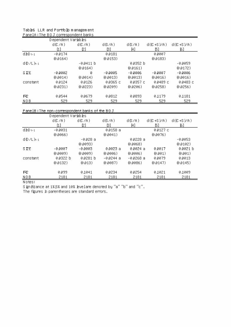
Table6　LLR and Portfolio managementPanel A: The BOJ correspondent banksp

Dependent Variablesd(C/A) d(C/A) d(S/A) d(S/A) d((C+S)/A) d((C+S)/A)[1] [2] [3] [4] [5] [6]

dlnDt-1 -0.0174 0.0181 0.0007(0.0164) (0.0153) (0.0183)

d(D/L)t-1 -0.0411 b 0.0352 b -0.0059(0.0164) (0.0161) (0.0172)

SIZE -0.0002 0 -0.0005 -0.0006 -0.0007 -0.0006SIZE 0.0002 0 0.0005 0.0006 0.0007 0.0006(0.0014) (0.0014) (0.0013) (0.0013) (0.0016) (0.0016)

constant 0.0124 0.0126 0.0365 c 0.0357 c 0.0489 c 0.0483 c(0.0231) (0.0223) (0.0209) (0.0206) (0.0258) (0.0256)

Ｒ2 0.0544 0.0679 0.0812 0.0893 0.1179 0.1181NOB 529 529 529 529 529 529

Panel B: The non-correspondent banks of the BOJPanel B: The non-correspondent banks of the BOJDependent Variablesd(C/A) d(C/A) d(S/A) d(S/A) d((C+S)/A) d((C+S)/A)[1] [2] [3] [4] [5] [6]

dlnDt-1 -0.0031 0.0158 a 0.0127 c(0.0066) (0.0041) (0.0076)

d(D/L)t-1 -0.028 a 0.0228 a -0.0053(0.0093) (0.0068) (0.0102)

SIZE 0 0007 0 0003 0 0023 0 0024 0 0017 0 0021 bSIZE -0.0007 -0.0003 0.0023 a 0.0024 a 0.0017 0.0021 b(0.0009) (0.0009) (0.0006) (0.0006) (0.001) (0.001)

constant 0.0322 b 0.0281 b -0.0244 a -0.0268 a 0.0079 0.0013(0.0132) (0.013) (0.0087) (0.0086) (0.0147) (0.0145)

Ｒ2 0.099 0.1041 0.0234 0.0254 0.1021 0.1009NOB 2181 2181 2181 2181 2181 2181Notes:

" " " " " "Significance at 1%,5% and 10% level are denoted by "a" "b" and "c".The figures in parentheses are standard errors.