Supporting Information

Table of contents Page

S1 Methods and data 2S1.1 Structural Decomposition Analysis 2S1.2 Data sources and processing 3S1.3 Structural Path Decomposition 4S1.4 Supply-Use tables 5

S2 Dealing with discontinuities in the time series and price changes 6S2.1 Discontinuities 6S2.2 Conversion to constant prices 9S2.3 Visualisation of discontinuities 11

S3 Mis-allocation in the supply-use framework 15

S4 Comparison with Wachsmann et al 16

S5 Sector classification 17S5.1 55 industries and 110 products (English) 17S5.2 12 value added and 6 final demand categories 19S5.3 55 industries and 110 products (Portuguese) 20S5.4 12 value added and 6 final demand categories 22

S6 Detailed results 23S6.1 ‘Beef cattle’ ’Meat products’ + ’Restaurants’ + ’Other food products’

+ ’Beef cattle’ ’Household consumption’ 24S6.2 ‘Beef cattle’ Beef cattle’ Capital formation’ 25S6.3 ‘Beef cattle’ ’Meat products’ ’Exports’ 26S6.4 ‘Soybeans’ ’Soybeans’ ’Exports’ 27S6.5 ‘Transport’ Passenger transport’ ’Household consumption’ 28S6.6 ‘Pig iron and alloys’ ’Pig iron and alloys’ ’Exports’ 29S6.7 Top-ranking structural paths driving change in CO2 emissions above

450 kilotonnes 30S6.8 All paths 34S6.9 Production-side structural decomposition analysis 36S6.10 Annual SDA results 37

S7 Structure of final demand 39

S8 Emission factors 40S.8.1 English 40S.8.2 Portuguese 41

Supporting Information References 42

1

S1 Methods and data

S1.1 Structural Decomposition Analysis

In this work we utilise Structural Decomposition Analysis (SDA), which is a technique commonly used for identifying drivers underlying change in an economy over time 1,2. It has been applied in numerous case studies on changes in economic variables 3, energy consumption 4, and nitrogen flows 5, but lately more often on changes in emissions 6-10. SDA requires at least a time series of input-output (IO) tables, but also works on IO systems including physical satellite accounts 11. A detailed introductory description of this technique can be found elsewhere 12. CO2

emissions from energy use in Brazil have been decomposed previously using Index Decomposition Analysis 13. Our study is significantly more detailed in that it offers sectoral detail, and also includes emissions from land use change.

In this work we decompose changes in Brazil’s total CO2 emissions E, and split those into six driving forces: changes in

- emissions intensity (eg due to technological progress), - production structure (eg due to re-organisation of supply-chains and industrial production

recipes), - demand composition (eg due to shifts to more meat-based diets), - demand destination (eg due to domestic market – exports shifts; consumption – investment

shifts), - demand level (eg due to increases in per-capita consumption expenditure), and - population (due to growth),

according to

∆ E=∆ eLuv yP⏟

Intensity

+e∆ Luv yP⏟∏ struct

+eL∆uv yP⏟Demcompos

+eLu ∆v yP⏟Demdestin

+eLuv ∆ yP⏟Demlevel

+eLuv y ∆ P⏟Population

,(1)

where e is a 1N vector of CO2 emission intensities for N industry sectors, L = (I – A)-1 is the NN Leontief inverse of the NN input coefficients matrix A = Tx̂−1, the hat symbol ‘^’ denotes a diagonalised vector, I is an NN identity matrix, T is an NN matrix of intermediate (supply-use, see SI S1.4) transactions, x = T1T + y1y is N1 economic gross output, 1T and 1y are N1 and M1 summation operators {1,1,…,1}t for NN intermediate transactions T (destined for further processing) and NM final demand y (destined for final consumption of households, the government, non-profit institutions, the capital sector, stocks, and exports), the NM matrix u =

y 1̂T y−1 holds the sectoral structure of final demand (NM matrix y normalised by its MM

column sums 1̂T y), the M1 matrix v = (1T y )tY−1 holds the destination structure of final

demand, the scalar y = 1T y 1yP−1 is total per-capita final demand, and P is population 14. The

superscript ‘t’ denotes vector transposition, whilst the superscript ‘T’ denotes a T-sized summation operator.

Inversion of I – A in supply-use form can proceed without conversion to a symmetrical input-output table, and yields Leontief multipliers Lij for industries and products simultaneously 15. We

2

use the SDA method described by 2 (average of all first order decompositions) because it is exact (i.e. leaves no residual) and non-parametrical 16, as well as zero-robust 17.

S1.2 Data sources and processing

In our SDA we use matrices T available as a supply-use table time series expressed in constant 2009R$ (see SI S2.2) that stretches the period 1970 to 2008, and that distinguishes 55 industries, 110 products and 6 final demand destinations, so that N = 165 and M = 6 18.

CO2 emission intensities e related to energy use were calculated on the basis of the Brazilian national energy balance 19. In a first step, fuel data in the energy balance were transformed into an energy satellite account. This was achieved by mapping the sector classification in the energy balance into that of the sector classification in the input-output tables using a concordance matrix (see Excel file in Supporting Information). In a second step, the energy satellite account was converted into an emissions satellite accounts based on detailed emission factors (SI S8).

Emissions from land use change were estimated using the approach of 20, with updated estimates on deforestation rates and carbon stocks (INPE, 2012; Zaks et al., 2009). This methodology takes an atmospheric-flow approach and allocates carbon emissions when there is a flow of carbon from the cleared biomass to the atmosphere. The deforested biomass is partitioned into a fraction oxidized immediately (20%), slash (70%), products (8%), and elemental carbon (2%), and each partition decays at a different rate. Net emissions were estimated taking into account regrowth taking place on previously deforested land (secondary forests). We assumed zero deforestation before 1960 in line with 20. As a consequence, the majority of emissions (about 80%) occur in a year later than the year of deforestation due to different decay constants of each partition leading to the concept of “legacy emissions” 21.

Although there are several uncertainties in the way emissions are estimated from deforestation 20, we use updated parameters (carbon density and deforestation rates) in an effort to decrease uncertainties 22,23. Ramankutty et al and Aguiar et al explore many of the uncertainties that arise in the model we use and find that biomass density maps, parameterizations of the dynamics such as secondary vegetation, and the fate of the deforestation land to be important. While these uncertainties are known, lack of data currently precludes reducing these uncertainties. Irrespective of these uncertainties in estimating the emissions from deforestation, the goal of the study is to understand the socio-economic drivers behind the deforestation, and for this, a robust baseline is needed to attribute emissions to producers and consumers who may use deforested land. In other words, improved estimates of the emissions from deforestation will not change the drivers of land use, but it will affect the share of emissions allocated to fossil fuels compared to land use change.

The deforested area and the associated emissions were allocated to products from cropland (soybeans) and pasture (cattle meat) based on direct land use change. The share allocated to soybeans and cattle meat is based on estimates of land use transitions after deforestation. In this modeling framework, a share of the emissions are allocated to cropland and cattle meat in the year of deforestation, but in each subsequent year the land use either remains the same or changes to cropland, pastures, or secondary forests 20. The estimates of direct land use change and land use transitions are grounded in field studies and satellite observations 24-26, though

3

they are extrapolated to a larger area and thus remain highly uncertain. In Brazil most soybean production and cattle ranching occurs on newly or previously deforested areas, making the allocation of emissions to all soybean products and cattle meat reasonable 24.

Our allocation of deforested area and the associated emissions to sectors is based on direct land use change 27. In direct land use change, the allocation is based on the actual land use that occurs on the deforested land and consequently can be observed 28. It is also possible to consider indirect land use change, where increased demand for agricultural products on existing agricultural land may displace an existing agricultural product and cause land use change elsewhere 27. Indirect land use change is most commonly applied in the analysis of biofuels 29,30 though it is equally relevant for other drivers. Indirect land use change is generally based on modelling, with differing assumptions leading to significantly different results 31. Our analysis is based on historical developments (from 1970 to 2008), where changes due to the more recent biofuel policies are unlikely to have had any effect. While it may be that in the past (pre-2008) deforestation has been driven by indirect land use change, we are not aware of literature that supports this. Thus, we base our analysis on direct land use change. Extending our analysis into the future would require the inclusion of indirect land use change.

S1.3 Structural Path Decomposition

Structural Decomposition Analysis (SDA) in itself yields results that are too coarse to inform about drivers at the level of economic agents, products or industries. We therefore employ Structural Path Decomposition (SPD; Wood and Lenzen, 2009), which extends SDA in that it allows extracting agent, industry and product information from aggregates in Eq. 1, as

∆ E=∑ijk∆ei Liju jk vk yP⏟

Intensity

+∑ijkei∆ Liju jk vk yP⏟Production structure

+∑ijke iLij∆u jk vk yP⏟Demand composition

+…

+∑ijke iLiju jk∆ vk yP⏟Demand destination

+∑ijke iLiju jk vk∆ yP⏟Demand level

+∑ijkei Lij u jk vk y ∆P⏟

Population

, (2)

where each term d e ijk=∆ei Liju jkvk YP, d Lijk=ei∆ Liju jk vk YP, and so on, describes a structural change Ei in Ei along a particular path {i,j,k} connecting a CO2-emitting industry i with a product j supplied to final demand destination k. The emitting industry i can, but need not be the supplier of product j. For example, a steel manufacturer i could be at the producing end of a path, delivering steel to a steel sheet rolling facility that in turn supplies a manufacturer of a car that in turn is purchased by an insurance company that sells policies j to households. This and other possible paths linking ‘Steel’ i and ‘Insurance’ j are included in the Leontief term Lij. In fact, the Leontief inverse L contains the entire supply chain network of the Brazilian economy, linking emissions and production on one hand, and final demand and consumption on the other. The final demand destinations k are economic agents such as households, the government, capital investors, and foreign entities importing from Brazil. The difference between Eq. 2 and the formulation in 32 is that in Eq. 2 the Leontief inverse L is not expanded into an infinite series. The series expansion is not pursued in this work because of limited policy options to affect individual supply stages in an economy’s production recipe.

4

S1.4 Supply-Use tables

The data underlying the Structural Decomposition Analysis are a time series of supply-use tables (SUTs) in a constant format (Fig. S1).

y

v

V

U

xi' xc'

xi

xc

m,tp

M My

m,tp

Fig. S1: Schematic of a supply-use table (SUT). The components are the supply matrix V, the use matrix U, final demand y, gross industry output xi, gross commodity (product) output xc, value added v, transport and trade margins m, taxes less subsidies on products tp, intermediate imports M, and final imports My.

The supply and use matrices hold the accounting entries for intermediate transactions where goods and services are received for further processing. Final demand ends with households, governments, or foreign entities. Value added and imports are considered primary inputs to the productive cycle, as they are not generated by domestic intermediate producers. Margins and product taxes are added onto transactions in basic prices, that is farm- or factory-gate prices, yielding purchasers’ prices. Supply-use tables are balanced in the sense that row and column sums both equal gross output x.

The intermediate transactions matrix T mentioned in the main text is equal to the supply-use

block [ 0 VU 0 ]. Such supply-use blocks are a standard feature of economic input-output analysis,

and are described for example in the United Nations’ Handbook on the compilation of input-output tables 33.

5

6

S2 Dealing with discontinuities in the time series and price changes

S2.1 Discontinuities

The time series used for the Structural Decomposition Analysis was assembled from six different data sources with tables expressed in six different classifications (1970, 1975, 1980, 1985-1996, 1995-1999, 2000-2008.18 This is due to a number of historical transitions in the structure and governance of the Brazilian National Accounts. Before 1986, annual macroeconomic estimates were projected on the basis of price and quantity data from isolated census years.34 In 1986, when Brazil’s National Accounts became the responsibility of the Brazil’s Geographical and Statistical Institute (IBGE), all post-1970 estimates were re-calculated in order to adhere to the United Nations System of National Accounts (SNA). This re-calculation involved some changes to the National Classification of Economic Activities (CNEA), with repercussions for the format of Brazil’s input-output tables.35 For example, from 1980 onwards, input-output tables adhere to production measures that include some estimate of the activity of the informal economy. From 1990 onwards, a new System of National Accounts (NSCN; introduced by the IBGE in 1997) is applied, with an increased focus on the internal consistency of macroeconomic accounts, input-output tables, and supply-use tables.36 From 2000 onwards, the IBGE incorporated additional primary data sources in its data collection, such as household income surveys, and government administration surveys.37 These historical circumstances lead to a number of breaks in the continuity of Brazil’s input-output database. Whilst these discontinuities can be severe at the sectoral level, they do not lead to imbalances of more than 2% of gross output (see Fig. S2.2). In the following we provide a detailed and exhaustive account of all discontinuities encountered, and corrections implemented.

1.4 1.5 1.6 1.7 1.8 1.9 2.0 2.1 2.2 2.3

1970 1980 1990 2000 2010

Gros

s out

put /

GDP

Year Wachsmann et al IBGE SUT IBGE TIP

Fig. S2.1: Ratio of gross output to GDP in the source data sets from Wachsmann et al 14, the official Supply-Use Tables (SUT) 38, and the official Input-Output Tables (Tabelas Insumo-Produto, TIP 39) . Reproduced from the Appendix in Lenzen et al 18.

7

First, the ratio between gross output and GDP, and hence the ratio between data components such as the supply matrix and the value-added block, are subject to sudden changes. This means for example that energy and emissions intensities e and c are comparatively large during 1997-1999, where the Supply-Use Tables with low gross output are being used (Fig. S2.1).

Second, a number of breaks in the definition of industry or product output occur. For example, in the original data for 1970 trade margins are accounted under the industry label ‘Distribution’ (‘Distribuição’). However, in 1975 the same industry featured a substantially smaller output, and a new industry ‘Trade’ (‘Comércio’) takes on the role of trade margins supplier.

Another example are sugar cane and refinery products, where in the original 1970 data ‘Alcohol’ (‘Álcool etílico’, from sugar cane or grains), ‘Petrol and diesel’ (‘Gasolina e óleo diesel’) and ‘Fuel oils’ (‘Óleos combustíveis’) are distinguished. In 1975, ‘Petrol’ and ‘Diesel’ appear disaggregated. In 1980, ‘Diesel’ becomes aggregated with ‘Fuel oils’, and ‘Petrol’ is split into ‘Pure petrol’ and ‘Automotive petrol’. From 1985 onwards, the distinction between two types of petrol disappears again, however a new type of fuel, ‘Gasoálcool’ is added. In addition, the product ‘Gasoálcool’ is produced by the industry ‘Petrol refining’ in 1985, and after 1995, but by the industry ‘Trade’ (‘Comércio’) between 1990 and 1994, leading to sharp breaks in the supply table. In order to accommodate these frequent changes, the supply-use table time series used in this work is expressed in a more detailed classification that contains five different fuels (‘Alcohol’, ‘Petrol’, ‘Diesel’, ‘Fuel oil’ and ‘Gasoalcohol’), and thus a well-defined relationship exists between this classification and those of all original tables issued by the Brazilian statistical agency IBGE. This disaggregation handles almost all discontinuity problems, however some manual adjustments of the final demand coefficients of the fuels listed above in the vector u needed to be made for the year 1970.

A further example is the transport modes, where in 1970 and 1975, freight and passenger transport are distinguished, but not thereafter. In contrast, education is disaggregated from an aggregate service sector only from 1975 onwards, and health is disaggregated only from 1980 onwards. In both examples, the classification used in this work distinguished the more disaggregated sectors (see SI S5). Given the energy- and CO2 intensity of the transport sector, we needed to correct the resulting discontinuities manually post-balancing. The provision of education is neither energy- nor CO2-intensive, and therefore we did not undertake any manual corrections.

Third, in some years, one or more fictitious “dummy” sectors are included in the original data (see Section 3.3 in Lenzen et al 18). We allocated the output of those dummy sectors to regular intermediate sectors with a similar output. In particular, we allocated the sizeable ‘Financial dummy’ (‘Dummy financeiro’) to the ‘Financial intermediation’ sector (‘Intermediação financeira e seguros’), causing some imbalances in the final demand (household and exports segments) of the latter sector, which we corrected manually.

Fourth, the IBGE tables for 1970, 1975, and 1980 include a forestry formation sector ‘Florestamento e formação de culturas permanentes’ that disappears from 1985 onwards. Within final demand, this sector records exclusively large fixed capital expenditures. Integration of this sector into the common forestry sector ‘Produtos da exploração florestal e da silvicultura’ therefore led to a significant discontinuity at the transition from 1980 to 1985. Given that the output of the forestry formation sector reflects only the value of forest assets, which are

8

inconsequential for energy and CO2 analyses, we manually reduced the fixed capital expenditure coefficients in the vector u to their average post-1985 level.

Fig. S2.2: Imbalances in the input-output balance of 55 industries (left) and 110 products (right) over time (compare industry and product list in SI S5). The first row of heat maps applies to the first backward balancing sweep from 2008 to 1970, the second row to the subsequent forward sweep from 1970 to 2008, and the third row shows the average of the first and second sweep. These balancing sweeps are averaged in order to deal with the problem of hysteresis when constructing the supply-use time series.18 The forward sweep starting 1970 shows larger imbalances because of the misclassifications and discontinuities in the early years.

Fifth, the original supply-use tables provided by the IBGE include some large negative changes in inventories in the final demand column, especially for raw agricultural products such as soy, corn and sugar cane. In some cases, large negative changes in inventories led to a reduction in gross output to an extent that elements in the input coefficients matrix A became too large for numerically stable inversion into the Leontief matrix L. We circumvented this problem by mirroring negative final-demand entries into positive value-added entries, and vice versa. Sixth, in 2000 the IBGE started to consider the increase in the number of cattle heads as a capital formation instead of as changes in stocks (personal communication Joaquim Guilhoto 17 August 2012). This change left the sum of capital formation and changes in stocks about constant over time (Fig. S2.3). Nevertheless, we found that the 2000 discontinuity for beef cattle distorted SDA results, mainly because of the high LUC emissions intensity of these products. We therefore

9

manually added changes in inventories to capital formation, and then set changes in inventories to zero. As a result this accounting discontinuity does not affect the SDA results described in the main text.

Fig. S2.3: Intermediate (solid line) and final demand (dashed line) of beef cattle between 1970 and 2008, with final demand broken down into capital formation (dash-dotted) and changes in stocks (dotted). Capital formation and changes in stocks changed roles in 2000.

S2.2 Conversion to constant prices

We converted the monetary entries in the Brazilian supply-use tables into constant 2009 R$ using inflators listed in Tab. 3 in Lenzen et al. 18 We then examined the temporal profile of gross output of for all industries and products in the supply-use tables, and searched particularly for sharp declines and increases. We found that the prices of some primary and basic secondary products experienced a sharp decline between 1995 and 2000, and a subsequent sharp increase between 2000 and 2005, with profound consequences for monetary quantities in the supply-use tables.40-42 Examples are basic steel and products fabricated thereof, and refinery products (Figs. S2.4 and S2.5), but also agricultural products such as beef cattle. The price changes of these products are considerably larger than the inflation rate of the whole economy. As a consequence, when adjusting the transaction values pertaining to such products we used Producer Price Indices. We applied the principle of double deflation, where imbalances in total use and total output are absorbed by value added to achieve the table balance. Hence, no further balancing was necessary after deflating the intermediate and final demand entries.43

10

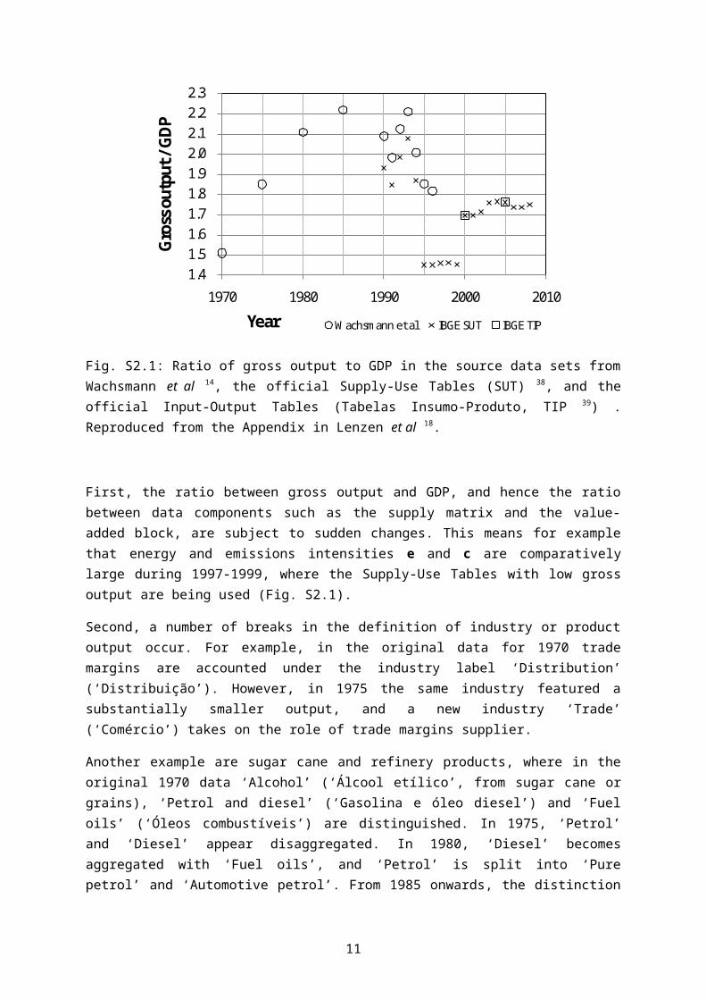
Fig. S2.4: Gross output of Brazilian refinery and steel products between 1970 and 2008, expressed in 2009 R$, but using only economy-wise inflators to convert to constant prices. The sharp dips spanning 1993 to 2004 are caused by above-average price movements.

Fig. S2.5: Ratio PPIi/PPIeconomy of Producer Price Indices (PPI) of industries i = {Refinery products, Steel products}41,42 and the entire economy40 between 1993 and 2008. The sharp dips spanning 1993 to 2004 are caused by product price decreases above the economy-wide average.

11

S2.3 Visualisation of discontinuities

Discontinuities can be visualised as heat maps of absolute changes (Fig. S2.6) and relative changes (Fig. S2.7) across supply-use sectors and years. Potentially critical are those instances with large relative changes (above 0.5 and below –0.5) and also large absolute changes.

For example, CO2 emissions and intensity changes quite abruptly for sector 26 (the ‘Refining’ industry), however in absolute terms these changes are negligible (note that fuels were allocated to various refinery products, not to the industry).15 There are also isolated large relative changes in gross output x and intermediate inputs U, and hence in the production recipes A and L, especially around 1975 and 1996; these relate to the discontinuities of the refinery products, trade and transport sectors described above. The heat map shows that such discontinuities are rather exceptions overall, and that their magnitude diminishes with the transformation of the production recipe A to the cumulative production recipe L.

Relative changes in final demand appear more pronounced, with values up to 200%, especially for products 55 to 80 (agriculture, forestry and mining) and 100 to 140 (heavy industries; paper, refining, chemicals, steel and steel products). These changes are mainly registered in the final demand destinations of changes in stocks (especially agriculture, forestry and mining), exports (soy, beef, sugar, coffee, metal semi-fabricates), and fixed capital (forestry and machines). Abrupt changes in the composition of household consumption (the most important destination of final demand) also occur, but rarely does a product represent more than 2% of total household consumption.

12

Fig. S2.6: Heat maps of absolute five-year changes of CO2 emissions (Ci), CO2 intensity (ci), gross output (xi), production recipe (jAij), intermediate inputs (iUij), cumulative production recipe (iLij), final demand (jYij), and composition of household consumption (uih), for 165 supply-use sectors (y-axis) and the period 1970-2008 (x-axis). Red means large positive change between subsequent years, blue large negative change. No change assumes different colours depending on the scale.

13

Fig. S2.7: Heat maps of relative five-year changes rel of CO2 emissions (Ci), CO2 intensity (ci), gross output (xi), production recipe (jAij), intermediate inputs (iUij), cumulative production recipe (iLij), final demand (jYij), and composition of household consumption (uih), for 165 supply-use sectors (y-axis) and the period 1970-2008 (x-axis). Red means large positive change between subsequent years, blue large negative change. No change assumes different colours depending on the scale.

14

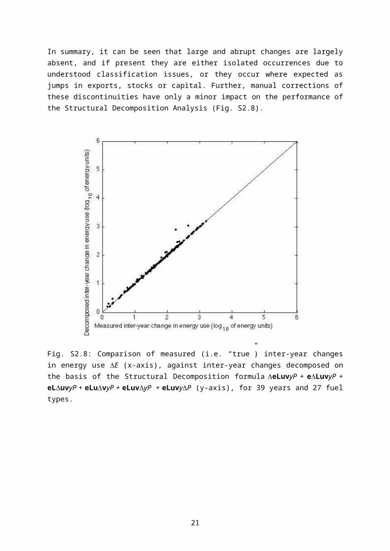
In summary, it can be seen that large and abrupt changes are largely absent, and if present they are either isolated occurrences due to understood classification issues, or they occur where expected as jumps in exports, stocks or capital. Further, manual corrections of these discontinuities have only a minor impact on the performance of the Structural Decomposition Analysis (Fig. S2.8).

Fig. S2.8: Comparison of measured (i.e. “true”) inter-year changes in energy use E (x-axis), against inter-year changes decomposed on the basis of the Structural Decomposition formula eLuvyP + eLuvyP + eLuvyP + eLuvyP + eLuvyP + eLuvyP (y-axis), for 39 years and 27 fuel types.

15

S3 Mis-allocation in the supply-use framework

When inverting the coefficients matrix I – A of the intermediate transactions block [ 0 VU 0 ] in

the supply-use system shown in SI S1.4, the resulting Leontief inverse is fully populated, that is its diagonal blocks are not zero anymore.15 In essence, the matrix multiplications implicit in the inversion of the supply-use block connect products with products, i.e. products that are used by industries that in turn produce other products. A particular shortcoming arises out of the fact that industries in the Brazilian supply-use classification are more aggregated (55) than products (110). For example, a range of agricultural products (rice in the husk, soybeans, wheat, manioc, cotton, coffee, tobacco, beef cattle, raw milk, sugar cane etc) are used by only one ‘Food products’ industry (‘Alimentos e bebidas’) that in turn produces a large range of food products (beef meat, pork, chicken meat, milk, sugar, flour etc). The fact that there is only one industry linking these two product ranges means that for example the use of beef cattle gets erroneously allocated to all food products. This behaviour cannot be corrected pre-inversion, i.e. inside the supply-use tables, unless one disaggregated the ‘Food products’ industry. We have dealt with this problem by making corrections directly in the Leontief matrix. For example, assume that i = beef cattle and j = {beef meat, pork, chicken meat, processed milk, sugar, wheat flour, manioc flour, tobacco products, cotton ginning, processed coffee}. For this example we would substitute the original Li1 with a new, corrected Li1,corr = Li1 + j=2,…,10 (Lij yj / y1), and set Lij,j=2,…,10 = 0 so that all connections between the beef cattle sector and non-beef-meat food sectors are severed. The scaling with final demand y is necessary because elements Lij of the Leontief inverse refer to total requirements per unit of final demand, and because gross output needs to be preserved. This can be seen using a 3-sector example:

x i=∑j=1

3

Lij y j=Li1 y1+Li2 y2+Li3 y3=(Li1+Li2 y2y1+Li3y3y1 ) y1+0 y2+0 y3 .

16

S4 Comparison with Wachsmann et al

Already in the early 1980s, Brazilian researchers undertook Structural Decomposition Analyses, mostly with income-distributional issues in mind, and remarkably only on the basis of two input-output tables.44,45 Only Wachsmann et al 14 have undertaken a more long-term Structural Decomposition Analysis, in their case of Brazil’s energy use between 1970 and 1996. Our study differs from that study because

- we analyse CO2 emissions in addition to energy use, and especially novel is our inclusion of CO2 emissions from land use change,

- we have extended the period to 2008,- instead of the Logarithmic Mean Divisia Index (LMDI46,47) method used by Wachsmann

et al 14 we use the SDA method by Dietzenbacher and Los2 because of the LMDI’s zero-value problems when applied to supply-use systems17,

- we use a more detailed industry and product classification (see SI S5),- we deal with hysteresis when constructing the supply-use time series, by averaging

between one forward and one backward iterative construction sweep18, for evidence see Fig. S2.2, and steps in Fig. S2.4 for the years 1970-1985),

- we use additional input data38, and- we deal with discontinuities and mis-allocation (see SI S3 and SI S4).

We compared our results on energy use with those reported in Wachsmann et al 14 for the period 1970-1996, and found only minor deviations (Fig. S4.1). We aggregated our supply-use tables into the classification used by Wachsmann et al 14, and found hardly any differences in the results. These SDA results are quite robust with regard to the method and data selection chosen, and therefore reasonable confidence can be placed in them.

Fig. S4.1: Comparison between Fig. 4 in Wachsmann et al 14 (1970-1996, left) and this work (1970-2008, right). N (left) corresponds to dq (right), and Pint to dP. Wachsmann’s Pres and r were not estimated in this study. Despite the differences listed above, SDA results for the first five sub-periods agree remarkably well.

17

S5 Sector classification

S5.1 55 industries and 110 products (English)

Industries Products

Agriculture and forestryGrazing and fishingCrude oil and natural gasIron oreOther minerals and oresFood and beveragesTobacco productsTextilesClothingLeather and footwearWood products except furnitureCellulose and paper productsNewspapers, magazines and electronic publishingPetroleum refining and coke productsAlcoholChemical productsResins and elastomersPharmaceutical productsPesticidesSoaps and detergentsInks, varnishes, enamels, lacquersOther chemical productsRubber and plastic productsCementOther non-metallic mineral productsManufacturing of steel and steel alloysNon-ferrous metalsFabricated metal products except machines and equipmentMachines and equipment, including maintenanceHousehold appliancesOffice equipmentElectric machines and materialsElectronic and communication equipmentMedical and optical equipmentPassenger and light utility vejiclesTrucks and bussesVehicle partsOther transport equipmentFurniture and other manufacturingElectricity, gas, water, sewerage and drainage servicesConstructionWholesale and retail tradeTransport and postal servicesInformation services

Rice in the huskCorn in the huskWheat grain and other cerealsSugar caneSoy grainOther product growingManiocTobacco leavesCottonCitrus fruitCoffeeForestry productsBeef and other live animalsMilk from cows and other animalsLive pigsLive birdsEggs of hens and other birdsFishing and aquacultureCrude oil and natural gasIron oreCoalNon-ferrous metallic mineralsNon-metallic mineralsAbattoirsPork meatChicken and other bird meatProcessed fishProcessed fruitOil, cakes, rind, flour and other raw soy productsOther vegetable oils except corn oilProcessed soy oilProcessed milkMilk productsRice and rice productsWheat flourManioc flourCorn oil manufacturing and other grain preparationsRefined sugarRoast and ground coffeeInstant coffeeOther food productsBeveragesTobacco productsCotton ginningWoven fabricsOther textile productsClothingLeather products except footwearFootwearWood products except furnitureCellulose for paper manufacturingPaper, cardboard and paper productsNewspapers, magazines, and electronic publishingLPGAutomotive petrolGasoalcoholFuel oilAutomotive Diesel OilOther refinery and coke productsAlcoholInorganic chemicalsOrganic chemicalsResin and elastomer products

18

Finance and insuranceProperty services and rentMaintenance and repairHotels and restaurantsBusiness servicesPrivate educationPrivate health servicesOther servicesPublic educationPublic health servicesPublic administration and social security

Pharmaceutic productsPesticidesSoaps and detergentsInks, varnishes, enamels, lacquersOther chemical productsRubber productsPlastic productsCementOther non-metallic mineral productsPig iron and iron alloysSemi-fabricates, laminates, bar and tubes of steelMetallurgic non-ferrous metal productsCast steelFabricated metal products except machines and equipmentMachines and equipment, including maintenanceHousehold appliancesOffice equipmentElectric machines and materialsElectronic and communication equipmentMedical and optical equipmentPassenger and light utility vehiclesTrucks and bussesVehicle partsOther transport equipmentFurniture and other manufacturingRecycled scrapElectricity, gas, water, sewerage and drainage servicesConstructionWholesale and retail tradeFreight transportPassenger transportPostal servicesInformation servicesFinance and insuranceProperty services and hiringImputed rentMaintenance and repairHotels and restaurantsBusiness servicesPrivate educationPrivate health servicesPersonal servicesServices rendered by associations and interest groupsHousehold servicesPublic educationPublic health servicesPublic administration and social security

S5.2 12 value added and 6 final demand categories (English)

Value added Final demand

Wages and salariesGovernment welfare (Fundo de Garantia do

Tempo de Serviço)Private welfareImputed social contributionsMixed gross incomeGross operating surplus

ExportsGovernment final

consumptionConsumption of Non-Profit

Institutions Serving Households (NPISH)

Household consumption

19

Other taxes on productionOther subsidies on productionTax on Circulation of Goods and Services

(Imposto sobre Circulação de Mercadorias e Prestação de Serviços)

Industrial products tax (Imposto sobre Produtos Industrializados) / Municipal tax on services (Imposto Sobre Serviços)

Other taxes on productsTaxes on imported products

Capital formationVariations in stocks

20

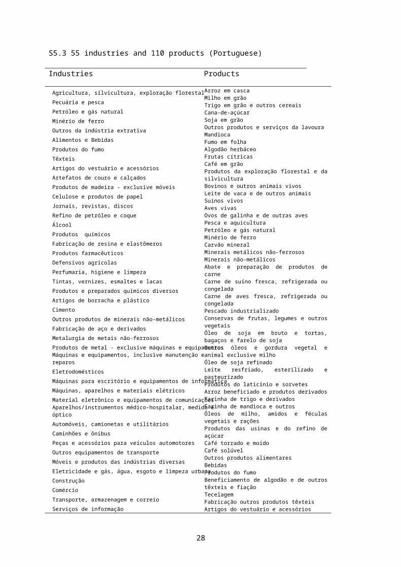
S5.3 55 industries and 110 products (Portuguese)

Industries Products

Agricultura, silvicultura, exploração florestalPecuária e pescaPetróleo e gás naturalMinério de ferroOutros da indústria extrativaAlimentos e BebidasProdutos do fumoTêxteisArtigos do vestuário e acessóriosArtefatos de couro e calçadosProdutos de madeira - exclusive móveisCelulose e produtos de papelJornais, revistas, discosRefino de petróleo e coqueÁlcoolProdutos químicosFabricação de resina e elastômerosProdutos farmacêuticosDefensivos agrícolasPerfumaria, higiene e limpezaTintas, vernizes, esmaltes e lacasProdutos e preparados químicos diversosArtigos de borracha e plásticoCimentoOutros produtos de minerais não-metálicosFabricação de aço e derivadosMetalurgia de metais não-ferrososProdutos de metal - exclusive máquinas e equipamentosMáquinas e equipamentos, inclusive manutenção e reparosEletrodomésticosMáquinas para escritório e equipamentos de informáticaMáquinas, aparelhos e materiais elétricosMaterial eletrônico e equipamentos de comunicaçõesAparelhos/instrumentos médico-hospitalar, medida e ópticoAutomóveis, camionetas e utilitáriosCaminhões e ônibusPeças e acessórios para veículos automotoresOutros equipamentos de transporteMóveis e produtos das indústrias diversasEletricidade e gás, água, esgoto e limpeza urbanaConstruçãoComércioTransporte, armazenagem e correioServiços de informaçãoIntermediação financeira e segurosServiços imobiliários e aluguel

Arroz em cascaMilho em grãoTrigo em grão e outros cereaisCana-de-açúcarSoja em grãoOutros produtos e serviços da lavouraMandiocaFumo em folhaAlgodão herbáceoFrutas cítricasCafé em grãoProdutos da exploração florestal e da silviculturaBovinos e outros animais vivosLeite de vaca e de outros animaisSuínos vivosAves vivasOvos de galinha e de outras avesPesca e aquiculturaPetróleo e gás naturalMinério de ferroCarvão mineralMinerais metálicos não-ferrososMinerais não-metálicosAbate e preparação de produtos de carneCarne de suíno fresca, refrigerada ou congeladaCarne de aves fresca, refrigerada ou congeladaPescado industrializadoConservas de frutas, legumes e outros vegetaisÓleo de soja em bruto e tortas, bagaços e farelo de sojaOutros óleos e gordura vegetal e animal exclusive milhoÓleo de soja refinadoLeite resfriado, esterilizado e pasteurizadoProdutos do laticínio e sorvetesArroz beneficiado e produtos derivadosFarinha de trigo e derivadosFarinha de mandioca e outrosÓleos de milho, amidos e féculas vegetais e raçõesProdutos das usinas e do refino de açúcarCafé torrado e moídoCafé solúvelOutros produtos alimentaresBebidasProdutos do fumoBeneficiamento de algodão e de outros têxteis e fiaçãoTecelagemFabricação outros produtos têxteisArtigos do vestuário e acessóriosPreparação do couro e fabricação de artefatos - exclusive calçadosFabricação de calçadosProdutos de madeira - exclusive móveisCelulose e outras pastas para fabricação de papelPapel e papelão, embalagens e artefatosJornais, revistas, discos e outros produtos gravadosGás liquefeito de petróleoGasolina automotivaGasoálcoolÓleo combustívelÓleo diesel

21

Serviços de manutenção e reparaçãoServiços de alojamento e alimentaçãoServiços prestados às empresasEducação mercantilSaúde mercantilOutros serviçosEducação públicaSaúde públicaAdministração pública e seguridade social

Outros produtos do refino de petróleo e coqueÁlcoolProdutos químicos inorgânicosProdutos químicos orgânicosFabricação de resina e elastômerosProdutos farmacêuticosDefensivos agrícolasPerfumaria, sabões e artigos de limpezaTintas, vernizes, esmaltes e lacasProdutos e preparados químicos diversosArtigos de borrachaArtigos de plásticoCimentoOutros produtos de minerais não-metálicosGusa e ferro-ligasSemi-acabacados, laminados planos, longos e tubos de açoProdutos da metalurgia de metais não-ferrososFundidos de açoProdutos de metal - exclusive máquinas e equipamentoMáquinas e equipamentos, inclusive manutenção e reparosEletrodomésticosMáquinas para escritório e equipamentos de informáticaMáquinas, aparelhos e materiais elétricosMaterial eletrônico e equipamentos de comunicaçõesAparelhos/instrumentos médico-hospitalar, medida e ópticoAutomóveis, camionetas e utilitáriosCaminhões e ônibusPeças e acessórios para veículos automotoresOutros equipamentos de transporteMóveis e produtos das indústrias diversasSucatas recicladasEletricidade e gás, água, esgoto e limpeza urbanaConstruçãoComércioTransporte de cargaTransporte de passageiroCorreioServiços de informaçãoIntermediação financeira e segurosServiços imobiliários e aluguelAluguel imputadoServiços de manutenção e reparaçãoServiços de alojamento e alimentaçãoServiços prestados às empresasEducação mercantilSaúde mercantilServiços prestados às famíliasServiços associativosServiços domésticosEducação públicaSaúde públicaServiço público e seguridade social

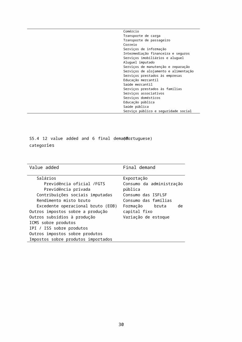
S5.4 12 value added and 6 final demand categories (Portuguese)

22

Value added Final demand

Salários Previdência oficial /FGTS Previdência privada Contribuições sociais imputadas Rendimento misto bruto Excedente operacional bruto (EOB)Outros impostos sobre a produçãoOutros subsídios à produçãoICMS sobre produtosIPI / ISS sobre produtosOutros impostos sobre produtosImpostos sobre produtos importados

ExportaçãoConsumo da administração públicaConsumo das ISFLSFConsumo das famíliasFormação bruta de capital fixoVariação de estoque

23

S6 Detailed results

In each of the following pages we will present two types of detailed results: 1) tables with Structural Path Decompositions (SPD), and 2) figures with trend analyses. Each table and figure will correspond to a particular supply chain path in the SPD, and these correspond to the fives paths contributing the largest changes.

The tables are structured as follows: The row headers of SPD tables show the final year of decomposition sub-periods, i.e. values in a row labelled ‘1975’ refer to effects occurring between 1970 and 1975. The column headers show the type of effect. The following abbreviations will be used throughout this subsection: de – Intensity effect, dL – Production structure effect, du – Demand structure effect, dv – Demand destination effect, dy – Demand level effect, and dP – Population effect. Values in tables are period-to-period changes due to a certain effect, expressed in Megatonnes (Mt) C02. Large increases of more than 20 Mt and large decreases of more than –20 Mt are printed in bold. Small changes between –5 Mt and 5 Mt are printed in italics. Empty fields mean that the respective value is smaller than 0.01.

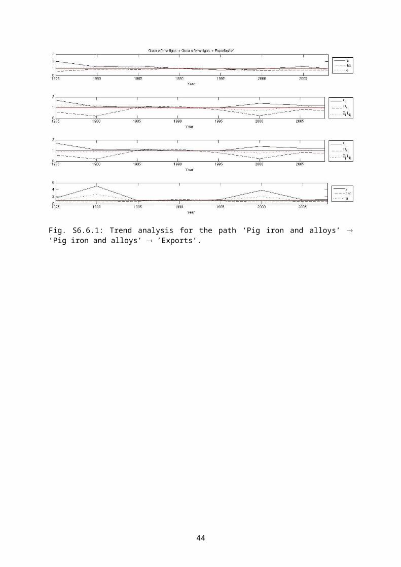
The figures are split into four panels and show the temporal changes in specific quantities. Trend graphs in the top panel show:

- period-to-period ratios of emissions E, with ratio Et+1 / Et plotted at year t+1,- period-to-period ratios of inverse gross output 1/x, with ratio xt / xt+1 plotted at year t+1,- period-to-period ratios of emission intensity e = E/x, with ratio et+1 / et plotted at year

t+1.

Similarly, trend graphs in the second panel show: - period-to-period ratios of gross output xi of the emitting sector i, - period-to-period ratios of final demand yi of the consumed product j, - period-to-period ratios of total requirements iLij of the consumed product j.

In the third panel they show: - period-to-period ratios of gross output xj of the consumed product j, - period-to-period ratios of final demand yi of the consumed product j, - period-to-period ratios of total requirements jLij of the emitting sector i.

The trend graphs in the bottom panel show: - period-to-period ratios of final demand yi of the consumed product j, - period-to-period ratios of total final demand Y of all consumed products, - period-to-period ratios of consumption shares u = yi/Y of the consumed product j.

24

S6.1 ‘Beef cattle’ ’Meat products’ + ’Restaurants’ + ’Other food products’ + ’Beef cattle’ ’Household consumption’

Year de dL du dv dy dP Total for period1975 15.9 3.8 -15.8 -6.5 15.5 6.5 19.41980 149.6 22.0 -20.7 18.3 42.6 15.2 226.91985 119.5 -26.0 -1.1 -28.4 -22.2 37.0 78.81990 -0.5 -0.2 -9.3 1.7 -7.1 36.1 20.71995 18.0 -47.0 -58.1 9.0 27.8 30.0 -20.22000 -43.1 -29.9 23.9 -1.8 47.0 28.0 24.22005 17.1 19.9 -22.5 -10.7 -8.0 27.1 22.82008 -80.0 -33.3 -5.8 -7.0 46.9 12.5 -66.7

Total for effect 196.5 -90.7 -109.5 -25.3 142.5 192.4 305.9

Tab. S6.1.1: Structural Path Decomposition for the sum of the four paths ‘Beef cattle’ ’Meat products’ ’Household consumption’, ‘Beef cattle’ ’Restaurants’ ’Household consumption’, ‘Beef cattle’ ‘Other food products’ ‘Household consumption’ and ‘Beef cattle’ ‘Beef cattle’ ‘Household consumption’. Large increases of more than 20 Mt and large decreases of more than –20 Mt are printed in bold. Small changes between –5 Mt and 5 Mt are printed in italics.

Fig. S6.1.1: Trend analysis for the path ‘Beef cattle’ ’Meat products’ ’Household consumption’.

25

S6.2 ‘Beef cattle’ Beef cattle’ Capital formation’

Year de dL du dv dy dP Total for period1975 16.8 -0.3 15.4 9.9 16.3 7.0 65.01980 188.0 2.6 -24.5 -40.2 52.1 18.5 196.51985 120.0 -1.8 -0.6 -54.9 -22.3 37.3 77.71990 -0.5 0.5 -39.1 -13.9 -6.6 34.0 -25.61995 14.5 -2.3 -133.0 -6.3 22.3 24.1 -80.72000 -28.9 0.9 11.9 -45.2 31.6 18.8 -10.92005 10.5 0.6 4.4 -29.9 -4.9 16.6 -2.72008 -49.5 -0.6 -13.9 6.3 29.0 7.7 -21.1

Total for effect 270.9 -0.4 -179.5-

174.3 117.4 164.0 198.2

Tab. S6.2.1: Structural Path Decomposition for the sum of the path ‘Beef cattle’ Beef cattle’ Capital formation’. Large increases of more than 20 Mt and large decreases of more than –20 Mt are printed in bold. Small changes between –5 Mt and 5 Mt are printed in italics.

Fig. S6.2.1: Trend analysis for the path ‘Beef cattle’ Beef cattle’ Capital formation’.

26

S6.3 ‘Beef cattle’ ’Meat products’ ’Exports’

Year de dL du dv dy dP Total for period1975 1.1 0.3 -2.2 0.3 1.1 0.5 1.11980 10.7 1.5 -1.4 2.4 3.1 1.1 17.31985 12.2 -1.8 9.8 6.3 -2.3 3.8 28.01990 0.0 -0.5 -24.5 -11.9 -0.6 3.0 -34.51995 0.9 -2.2 9.1 -0.8 1.4 1.6 10.02000 -3.4 -5.6 -0.1 11.7 3.6 2.2 8.52005 2.4 4.0 27.7 15.5 -1.2 3.8 52.32008 -17.2 -6.6 -3.7 4.6 10.1 2.7 -10.2

Total for effect 6.8 -10.9 14.7 28.0 15.3 18.6 72.5

Tab. S6.3.1: Structural Path Decomposition for the path ‘Beef cattle’ ’Meat products’ ’Exports’. Large increases of more than 5 Mt and large decreases of more than –5 Mt are printed in bold. Small changes between –1 Mt and 1 Mt are printed in italics.

Fig. S6.3.1: Trend analysis for the path ‘Beef cattle’ ’Meat products’ ’Exports’.

27

S6.4 ‘Soybeans’ ’Soybeans’ ’Exports’

This path includes the immediate export of harvested soybeans ‘s’ (es ys,export), but also intermediate routes such as soybeans for food ‘f’ for catering ‘c’ for insurance marketing events ‘i’ for the transport industries ‘t’ for soybean exports (es As,f Af,c Ac,i Ai,t At,s ys,export).

Year de dL du dv dy dP Total for period1975 5.1 -0.1 0.0 1.0 3.7 1.6 11.31980 30.0 0.1 -41.7 5.9 7.7 2.7 4.81985 -3.8 0.0 2.2 4.6 -1.7 2.8 4.21990 2.8 -0.1 -0.2 -9.8 -0.5 2.4 -5.41995 4.2 0.0 -9.9 -0.8 1.5 1.6 -3.42000 -30.9 0.1 46.5 16.0 5.1 3.0 39.82005 -8.7 0.3 1.8 18.1 -1.3 4.4 14.62008 -36.0 0.0 4.5 3.7 8.1 2.2 -17.6

Total for effect -37.3 0.3 3.2 38.7 22.6 20.7 48.2

Tab. S6.4.1: Structural Path Decomposition for the path ‘Soybeans’ ’Soybeans’ ’Exports’. Large increases of more than 5 Mt and large decreases of more than –5 Mt are printed in bold. Small changes between –1 Mt and 1 Mt are printed in italics.

Fig. S6.4.1: Trend analysis for the path ‘Soybeans’ ’Soybeans’ ’Exports’.

28

S6.5 ‘Transport’ Passenger transport’ ’Household consumption’

Year de dL du dv dy dP Total for period1975 -9.3 1.9 4.2 -2.1 5.2 2.2 2.11980 -6.7 -1.0 -0.7 1.9 4.5 1.6 -0.41985 4.9 0.5 1.5 -1.6 -1.3 2.1 6.01990

5.7 0.4-

2.7 0.1 -0.5 2.3 5.41995

7.2 -0.7-

3.7 0.7 2.3 2.5 8.32000 -3.5 -3.8 9.3 -0.2 5.0 3.0 9.82005

-5.0 0.9-

1.3 -1.2 -0.9 2.9 -4.42008

1.1 -0.1-

3.1 -0.8 5.3 1.4 3.8

Total for effect -5.7 -1.9 3.6 -3.1 19.718.

0 30.6

Tab. S6.5.1: Structural Path Decomposition for the path ‘Transport’ Passenger transport’ ’Household consumption’. Large increases of more than 5 Mt and large decreases of more than –5 Mt are printed in bold. Small changes between –1 Mt and 1 Mt are printed in italics. Empty fields mean that the respective value is smaller than 0.01.

Fig. S6.5.1: Trend analysis for the path ‘Transport’ Passenger transport’ ’Household consumption’.

29

S6.6 ‘Pig iron and alloys’ ’Pig iron and alloys’ ’Exports’

This path includes the immediate export of pig iron and alloys ‘p’ (ep yp,export), but also intermediate routes such as pig iron and alloys for steel ‘s’ for rolled sheet ‘r’ for vehicles ‘v’ for the transport industries ‘t’ for pig iron and alloys exports (ep Ap,s As,r Ar,v Av,t At,p yp,export).

Year de dL du dv dy dP Total for period1975 0.1 0.0 0.0 0.1 0.2 0.1 0.51980 0.5 -0.1 2.6 0.6 0.8 0.3 4.71985

1.1 0.0-

1.7 1.2 -0.4 0.7 0.91990 0.3 0.0 1.3 -2.6 -0.1 0.6 -0.51995 -1.1 0.0 0.6 -0.3 0.5 0.5 0.22000 -4.2 -0.1 8.2 4.6 1.4 0.9 10.82005

1.1 0.0-

2.4 5.5 -0.4 1.3 5.12008 -4.4 0.0 0.5 1.3 2.8 0.8 0.9

Total for effect -6.7 -0.2 9.1 10.3 4.8 5.2 22.6

Tab. S6.6.1: Structural Path Decomposition for the path ‘Pig iron and alloys’ ’Pig iron and alloys’ ’Exports’. Large increases of more than 5 Mt and large decreases of more than –5 Mt are printed in bold. Small changes between –1 Mt and 1 Mt are printed in italics. Empty fields mean that the respective value is smaller than 0.01.

Fig. S6.6.1: Trend analysis for the path ‘Pig iron and alloys’ ’Pig iron and alloys’ ’Exports’.

30

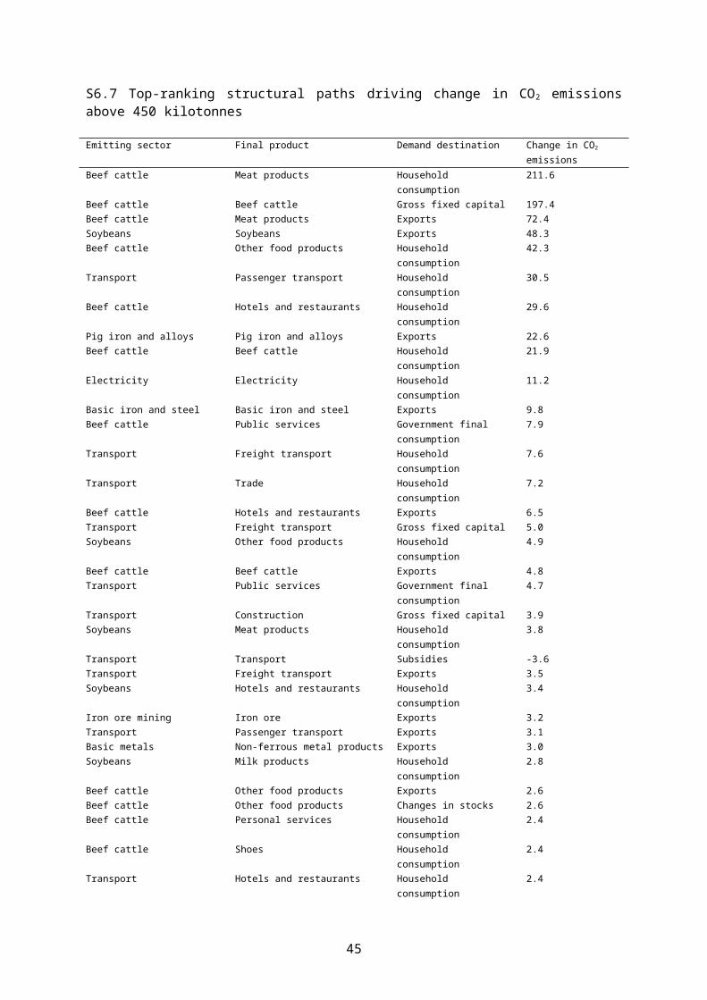
S6.7 Top-ranking structural paths driving change in CO2 emissions above 450 kilotonnes

Emitting sector Final product Demand destination Change in CO2 emissions

Beef cattle Meat products Household consumption 211.6Beef cattle Beef cattle Gross fixed capital 197.4Beef cattle Meat products Exports 72.4Soybeans Soybeans Exports 48.3Beef cattle Other food products Household consumption 42.3Transport Passenger transport Household consumption 30.5Beef cattle Hotels and restaurants Household consumption 29.6Pig iron and alloys Pig iron and alloys Exports 22.6Beef cattle Beef cattle Household consumption 21.9Electricity Electricity Household consumption 11.2Basic iron and steel Basic iron and steel Exports 9.8Beef cattle Public services Government final

consumption7.9

Transport Freight transport Household consumption 7.6Transport Trade Household consumption 7.2Beef cattle Hotels and restaurants Exports 6.5Transport Freight transport Gross fixed capital 5.0Soybeans Other food products Household consumption 4.9Beef cattle Beef cattle Exports 4.8Transport Public services Government final

consumption4.7

Transport Construction Gross fixed capital 3.9Soybeans Meat products Household consumption 3.8Transport Transport Subsidies -3.6Transport Freight transport Exports 3.5Soybeans Hotels and restaurants Household consumption 3.4Iron ore mining Iron ore Exports 3.2Transport Passenger transport Exports 3.1Basic metals Non-ferrous metal products Exports 3.0Soybeans Milk products Household consumption 2.8Beef cattle Other food products Exports 2.6Beef cattle Other food products Changes in stocks 2.6Beef cattle Personal services Household consumption 2.4Beef cattle Shoes Household consumption 2.4Transport Hotels and restaurants Household consumption 2.4Crude oil and natural gas Crude oil and natural gas Exports 2.4Soybeans Soy products Exports 2.3Basic iron and steel Machines Gross fixed capital 2.3Soybeans Beverages Household consumption 2.2Beef cattle Raw milk Household consumption 2.1Pig iron and alloys Construction Gross fixed capital -2.1Electricity Public services Government final

consumption2.0

Beef cattle Public education Government final consumption

2.0

Soybeans Chicken meat Exports 2.0Transport Machines Gross fixed capital 2.0Transport Private health care Household consumption 2.0Transport Vehicles Household consumption 1.9Transport Iron ore Exports 1.8Transport Meat products Household consumption 1.8Beef cattle Private health care Household consumption 1.8Beef cattle Alcohol Household consumption 1.8Beef cattle Household services Household consumption 1.7Beef cattle Interest groups Institutions serving

households1.7

31

Soybeans Chicken meat Household consumption 1.7Cement Construction Gross fixed capital 1.7Soybeans Meat products Exports 1.7Beef cattle Other agricultural products and

servicesHousehold consumption 1.6

Transport Other food products Household consumption 1.6Other non-metallic mineral products

Other non-metallic mineral products Exports 1.6

Basic iron and steel Machines Exports 1.6Soybeans Refined sugar Exports 1.6Beef cattle Public health care Government final

consumption1.5

Beef cattle Hygiene products Household consumption 1.5Transport Public health care Government final

consumption1.5

Transport Basic iron and steel Exports 1.5Transport Crude oil and natural gas Exports 1.5Soybeans Rice products Household consumption 1.5Crude oil and natural gas Gasoalcohol Household consumption 1.4Transport Personal services Household consumption 1.4Transport Trade Gross fixed capital 1.4Basic iron and steel Vehicles Household consumption 1.4Transport IT services Household consumption 1.4Beef cattle Fishing Household consumption 1.4Beef cattle Food products Subsidies -1.4Other non-metallic mineral products

Construction Gross fixed capital 1.3

Petroleum refining Gasoalcohol Household consumption 1.3Beef cattle Eggs Household consumption 1.3Transport Electricity Household consumption 1.3Transport Gasoalcohol Household consumption 1.3Transport Vehicles Exports 1.3Soybeans Vegetable oils Household consumption 1.2Soybeans Processed milk Household consumption 1.2Other refinery products Other refinery products Exports 1.2Transport Machines Exports 1.2Transport Postal services Household consumption 1.1Basic iron and steel Vehicles Exports 1.1Basic iron and steel Vehicle parts Exports 1.1Transport Public education Government final

consumption1.1

Agriculture and forestry Soybeans Exports 1.1Soybeans Refined soy oil Household consumption 1.1Beef cattle Clothing Household consumption 1.0Beef cattle Other textile products Household consumption 1.0Agriculture and forestry Other agricultural products and

servicesHousehold consumption 1.0

Transport Household services Household consumption 1.0Transport Private education Household consumption 1.0Transport Interest groups Institutions serving

households1.0

Pig iron and alloys Pig iron and alloys Changes in stocks 1.0Beef cattle Shoes Exports 1.0Transport Milk products Household consumption 1.0Beef cattle Trade Household consumption 1.0Transport Vehicles Gross fixed capital 1.0Transport Clothing Household consumption 1.0Electricity Trade Household consumption 1.0Beef cattle Construction Gross fixed capital 1.0Beef cattle Furniture Household consumption 0.9

32

Soybeans Public services Government final consumption

0.9

Beef cattle Alcohol Exports 0.9Beef cattle Private education Household consumption 0.9Electricity Public education Government final

consumption0.9

Transport Pharmaceutical products Household consumption 0.9Transport Soy products Exports 0.9Transport Beverages Household consumption 0.8Beef cattle Soybeans Exports 0.8Transport Non-ferrous metal products Exports 0.8Basic iron and steel Other metal prodcuts Gross fixed capital 0.8Soybeans Coffee Household consumption 0.8Transport Electronic equipment Gross fixed capital 0.8Transport Vehicle parts Exports 0.8Transport Hygiene products Household consumption 0.8Electricity Construction Gross fixed capital 0.8Basic iron and steel Other transport equipment Exports 0.8Soybeans Hotels and restaurants Exports 0.8Transport Furniture Household consumption 0.7Transport Trade Exports 0.7Transport Rice products Household consumption 0.7Soybeans Fruit and vegetable products Exports 0.7Soybeans Other agricultural products and

servicesHousehold consumption 0.7

Basic iron and steel Vehicles Gross fixed capital 0.7Transport Other agricultural products and

servicesHousehold consumption 0.7

Petroleum refining Petrol Household consumption -0.7Beef cattle Leather products Exports 0.7Cement Cement Household consumption 0.7Transport Chicken meat Exports 0.7Soybeans Manioc flour Household consumption 0.7Electricity Personal services Household consumption 0.7Transport Other metal prodcuts Gross fixed capital 0.6Basic iron and steel Household appliances Household consumption 0.6Electricity Private health care Household consumption 0.6Soybeans Oils and fats Household consumption 0.6Pharmaceutical products Pharmaceutical products Household consumption 0.6Pig iron and alloys Vehicle parts Exports 0.6Food products Other food products Household consumption 0.6Transport Trucks and buses Gross fixed capital 0.6Transport Chicken meat Household consumption 0.6Soybeans Fruit and vegetable products Household consumption 0.6Transport Meat products Exports 0.6Soybeans Refined sugar Household consumption 0.6Transport Refined sugar Exports 0.6Other refinery products Passenger transport Household consumption 0.6Transport Real estate Household consumption 0.6Transport Passenger transport Institutions serving

households-0.6

Transport Passenger transport Government final consumption

-0.6

Transport Shoes Household consumption 0.6Transport Pig iron and alloys Exports 0.6Electricity Machines Gross fixed capital 0.6Electricity Hotels and restaurants Household consumption 0.6Transport Other transport equipment Exports 0.6Agriculture and forestry Coffee Exports 0.6Transport Processed milk Household consumption 0.5

33

Electricity Non-ferrous metal products Exports 0.5Transport Household appliances Household consumption 0.5Beef cattle Real estate Household consumption 0.5Basic metals Machines Gross fixed capital 0.5Transport Soybeans Exports 0.5Crude oil and natural gas Passenger transport Household consumption 0.5Crude oil and natural gas Fuel oil Exports 0.5Electricity Public health care Government final

consumption0.5

Transport Hotels and restaurants Exports 0.5Electricity Basic iron and steel Exports 0.5Food products Wheat flour Household consumption -0.5Petroleum refining Fuel oil Exports 0.5Beef cattle Live birds Household consumption 0.5Government administration Public services Government final

consumption0.5

Transport Electronic equipment Household consumption 0.5Beef cattle Passenger transport Household consumption 0.5Hygiene products Hygiene products Household consumption 0.5Electricity Household services Household consumption 0.5Transport Fuel oil Exports 0.5Wood products Wood products Exports 0.5

Tab. S6.7.1: Top-ranking structural paths driving change in CO2 emissions above 500 kilotonnes. The top six structural paths are described in detail in Sections S6.1 – S6.6.

34

S6.8 All paths

Year de dL du dv dy dP Total for period1975 -3.9 44.9 -1.3 8.7 89.0 37.4 174.81980 463.5 72.1 -141.4 -12.1 186.4 65.9 634.41985 263.4 -44.1 31.3 -76.3 -75.9 126.8 225.31990 51.2 -25.8 -73.7 -84.5 -22.7 116.9 -38.51995 110.1 -82.2 -207.0 10.6 88.7 95.8 16.02000 -210.5 -75.4 34.1 8.0 151.6 90.2 -2.12005 0.0 65.9 9.0 6.6 -25.4 85.9 142.12008 -237.8 -74.1 -22.6 11.9 159.9 42.4 -120.4

Total for effect 436.0

-118.7 -371.5

-127.1 551.7 661.3 1031.7

Tab. S6.8.1: Structural Path Decomposition for the entire economy, and companion data to Fig. 2 in the main text. Large increases of more than 50 Mt and large decreases of more than –50 Mt are printed in bold. Small changes between –10 Mt and 10 Mt are printed in italics. Small discrepancies between Fig. 1 (main text, middle panel) and Fig. 2 (main text, and data in this table) are due to corrections made to the time series (SI S2 and S3, and Fig. S2.7).

Year de dL du dv dy dP Total for period1975 51.8 2.7 -4.2 4.9 47.0 19.9 122.11980 492.9 50.5 -130.0 -9.7 137.1 48.8 589.71985 254.1 -37.1 24.1 -72.9 -62.3 104.0 209.91990 14.9 -21.2 -69.4 -61.3 -18.7 95.6 -60.11995 70.1 -52.5 -194.0 12.0 70.4 76.0 -18.02000 -203.4 -53.0 27.6 -3.7 114.9 68.4 -49.22005 14.2 41.1 12.7 -4.7 -18.9 63.6 108.12008 -240.7 -56.1 -20.9 7.9 114.0 30.3 -165.4

Total for effect 454.0

-125.5 -354.1

-127.5 383.6 506.6 737.2

Tab. S6.8.2: Structural Path Decomposition for the entire economy, due to land use changes related to beef cattle grazing and soy cultivation. Large increases of more than 50 Mt and large decreases of more than –50 Mt are printed in bold. Small changes between –10 Mt and 10 Mt are printed in italics.

35

Year de dL du dv dy dP Total for period1975 -55.7 42.1 2.9 3.9 42.0 17.5 52.71980 -29.4 21.6 -11.5 -2.4 49.3 17.1 44.71985 9.3 -7.1 7.2 -3.4 -13.6 22.8 15.31990 36.3 -4.5 -4.2 -23.2 -4.0 21.3 21.61995

40.0-

29.6 -13.0 -1.4 18.3 19.8 34.12000

-7.1-

22.4 6.5 11.7 36.7 21.8 47.12005 -14.3 24.8 -3.7 11.3 -6.5 22.3 33.92008

2.9-

18.0 -1.7 3.9 45.9 12.1 45.1

Total for effect -18.0 6.8 -17.5 0.4168.

1 154.7 294.5

Tab. S6.8.3: Structural Path Decomposition for the entire economy, due to use of fossil energy carriers. Large increases of more than 50 Mt and large decreases of more than –50 Mt are printed in bold.

36

S6.9 Production-side structural decomposition analysis

Fig. S6.9.1: Production-side equivalent of Fig. 2 in the main text. Shades of column segments indicate broad emitting industries, rather than consumed products. Naturally, in this perspective, more importance is placed on primary industries such as agriculture and resource extraction.

37

S6.10 Annual SDA results

The results of any SDA will depend on the nature of the reporting periods chosen; such dependence is inevitable since there exist sub-period trends, and the net effect of these sub-period trends will depend on the temporal window applied. SDA results are usually not presented on an annual basis, because annual fluctuations are more affected by discontinuities and temporally isolated effects, and therefore less significant for long-term trend recognition and corresponding decision-making. In order to provide further detail on the results presented in Fig. 2, we ran SDA calculations on an annual basis between 1970 and 2008 (Fig. 6.10.1).

SDA results appear rather stable except for the period 1995 to 2000, and the year 2005. As described in Section 2, the 1995-2000 period is characterised both by revisions to Brazil’s National Accounts framework undertaken by the IBGE, as well as by relatively high inflation of the economy and non-average price changes of particular commodities. As a result, estimates of gross output are less reliable for this 1995-2000 period. This uncertainty affects the intensity and production structure effects, since both these effects incorporate gross output. It may therefore be that large, opposite intensity and structural effects are partly the result of discontinuities in gross output that simultaneously affect the intensity and structural terms in opposite directions. This could especially apply to the years 1995 and 2005. On the other hand, final demand and population effects are rather unaffected by the discontinuities described.

38

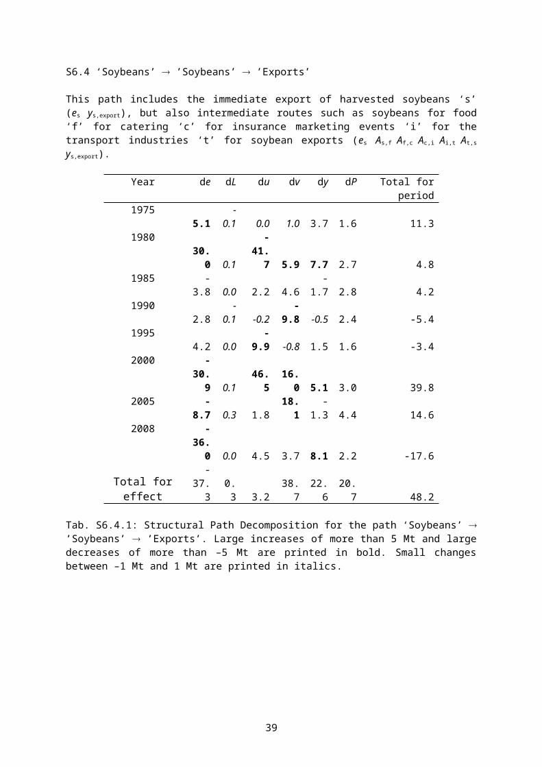
Fig. S6.10.1: Structural decomposition analysis (SDA) of the 1970-2008 CO2 emissions increase shown in the middle panel of Fig. 1 in the main text into six driving forces. Unlike in Fig. 2 in the main text, the bars in this figure represent changes over annual periods.

39

S7 Structure of final demand

Fig. S7.1: Contribution of various destinations to total final demand (in monetary terms). The spectacular increase of government final consumption over time stands out, and to a lesser extent the growth of exports and the decline of capital formation.

40

S8 Emission factors

S.8.1 English

CO2 content (g/MJ)

Crude oil 0Natural gas 51.3Steaming coal 90.0Metallurgic coal 0Uranium U3O8 0Hydraulic energy 0Wood 94.0Sugar cane products 96.8Other primary energy carriers 0Diesel oil 69.7Fuel oil 73.3Gasoline 66.0LPG 59.4Naphtalene 68.6Kerosene 69.7Town and coking gas 59.0Coke 90.0Uranium UO2 0Electricity 0Charcoal 90.0Alcohol 68.6Other secondary energy carriers

68.6

Non-energy crude oil products 0Tar 0

Tab. S8.1: Emission factors of energy carriers listed in the Brazilian National Energy Balance

We reduced emission factors by the degree to which the energy carrier was produced from renewable resources. We applied a reduction of 50% to wood (lenha), 50% to charcoal (carvão vegetal), and a reduction of 100% to bagasse (produtos da cana). From 2008 onwards, diesel (óleo diesel) included 2% biodiesel 48, whereas during the entire 1970-2008 period gasoline (gasoline) included a percentage of ethanol varying between 15% and 25%.49

41

S.8.2 Portuguese

CO2 content (g/MJ)

PETRÓLEO 0GÁS NATURAL 51.3CARVÃO VAPOR 90.0CARVÃO METALÚRGICO 0URÂNIO U3O8 0ENERGIA HIDRÁULICA 0LENHA 94.0PRODUTOS DA CANA 96.8OUTRAS FONTES PRIMÁRIAS 0ÓLEO DIESEL 69.7ÓLEO COMBUSTIVEL 73.3GASOLINA 66.0GLP 59.4NAFTA 68.6QUEROSENE 69.7GÁS DE CIDADE E DE COQUERIA 59.0COQUE DE CARVÃO MINERAL 90.0URÂNIO CONTIDO NO UO2 0ELETRICIDADE 0CARVÃO VEGETAL 45.0ÁLCOOL ETÍLICO ANIDRO E HIDRATADO 68.6OUTRAS SECUNDÁRIAS DE PETRÓLEO 68.6PRODUTOS NÃO ENERGÉTICOS DE PETRÓLEO

0

ALCATRÃO 0

Tab. S8.2: Emission factors of energy carriers listed in the Brazilian National Energy Balance

42

Supporting Information References

1 Rose, A. & Casler, S. Input-output structural decomposition analysis: a critical appraisal. Economic Systems Research 8, 33-62 (1996).

2 Dietzenbacher, E. & Los, B. Structural decomposition techniques: sense and sensitivity. Economic Systems Research 10, 307-323 (1998).

3 Skolka, J. Input-output structural decomposition analysis for Austria. Journal of Policy Modeling 11, 45-66 (1989).

4 Chen, C.-Y. & Rose, A. A structural decomposition analysis of changes in energy demand in Taiwan: 1971-1984. Energy Journal 11, 127-146 (1990).

5 Wier, M. & Hasler, B. Accounting for nitrogen in Denmark - a structural decomposition analysis. Ecological Economics 30, 317-331 (1999).

6 Casler, S. D. & Rose, A. Structural decomposition analysis of changes in greenhouse gas emissions in the U.S. Environmental and Resource Economics 11, 349-363 (1998).

7 Wier, M. Sources of changes in emissions from energy: a structural decomposition analysis. Economic Systems Research 10, 99-112 (1998).

8 De Haan, M. A structural decomposition analysis of pollution in the Netherlands. Economic Systems Research 13, 181-196 (2001).

9 Wood, R. Structural decomposition analysis of Australia's greenhouse gas emissions. Energy Policy 37, 4943-4948 (2009).

10 Yamakawa, A. & Peters, G. Structural Decomposition Analysis of greenhouse gas emissions in Norway 1990-2002 Economic Systems Research 23, 303-318 (2011).

11 Hoekstra, R. & van den Bergh, J. C. J. M. Structural decomposition analysis of physical flows in the economy. Environmental and Resource Economics 23, 357-378 (2002).

12 Rose, A. in Handbook of Environmental and Resource Economics (ed J. C. J. M. van den Bergh) 1165-1179 (Edward Elgar, 1999).

13 Medeiros, H. & Dezidera, D. Emissões de CO2 na Economia Brasileira: uma análise de decomposição. Revista Brasileira de Energia 12, 1-8 (2006).

14 Wachsmann, U., Wood, R., Lenzen, M. & Schaeffer, R. Structural decomposition of energy use in Brazil from 1970 to 1996. Applied Energy 86, 578-587 (2009).

15 Lenzen, M. & Rueda-Cantuche, J. M. A note on the use of supply-use tables in impact analyses. Statistics and Operations Research Transactions 36, 139-152 (2012).

16 Lenzen, M. Structural Decomposition Analysis and the Mean-Rate-of-Change Index. Applied Energy 83, 185–198 (2006).

17 Wood, R. & Lenzen, M. Zero-robustness of the Logarithmic Mean Divisia Index. Energy Policy 34, 1326-1331 (2004).

18 Lenzen, M., Pinto de Moura, M. C., Geschke, A., Kanemoto, K. & Moran, D. D. A cycling method for constructing input-output table time series from incomplete data. Economic Systems Research 24, 413-432 (2012).

19 EPE. Balanço Energético Nacional 2010 - Matrizes consolidadas. Report No. http://ben.epe.gov.br, (Empresa de Pesquisa Energética, Ministéria de Minas e Energia, Governo Federal, 2011).

20 Ramankutty, N. et al. Challenges to estimating carbon emissions from tropical deforestation. Global Change Biology 13, 51-66, doi:10.1111/j.1365-2486.2006.01272.x (2007).

21 Karstensen, J., Peters, G. P. & Andrew, R. M. Attribution of CO2 emissions from Brazilian deforestation to consumers between 1990 and 2010. Environmental Research Letters 8, 024005 (2013).

22 INPE. Brazil's National Institute for Space Research. Report No. http://www.inpe.br, (2012).

23 Zaks, D. P. M., Barford, C. C., Ramankutty, N. & Foley, J. A. Producer and consumer responsibility for greenhouse gas emissions from agricultural production - a perspective from the Brazilian Amazon. Environmental Research Letters 4, 044010 (2009).

43

24 Barona, E., Ramankutty, N., Hyman, G. & Coomes, O. T. The role of pasture and soybean in deforestation of the Brazilian Amazon. Environmental Research Letters 5, 024002 (2010).

25 Fearnside, P. M. Amazonian deforestation and global warming: carbon stocks in vegetation replacing Brazil's Amazon forest. Forest Ecology and Management 80, 21-34, doi:10.1016/0378-1127(95)03647-4 (1996).

26 Houghton, R. A. Carbon emissions and the drivers of deforestation and forest degradation in the tropics. Current Opinion in Environmental Sustainability, doi:10.1016/j.cosust.2012.06.006 (2012).

27 Searchinger, T. D. Biofuels and the need for additional carbon. Environmental Research Letters 5, 024007 (2010).

28 Morton, D. C. et al. Cropland expansion changes deforestation dynamics in the southern Brazilian Amazon. Proceedings of the National Academy of Sciences 103, 14637-14641, doi:10.1073/pnas.0606377103 (2006).

29 Fargione, J., Hill, J., Tilman, D., Polasky, S. & Hawthorne, P. Land Clearing and the Biofuel Carbon Debt. Science 319, 1235-1238, doi:10.1126/science.1152747 (2008).

30 Searchinger, T. et al. Use of US croplands for biofuels increases greenhouse gases through emissions from land use change. Science 319, 1238–1240 (2008).

31 IPCC. Special Report on Renewable Energy Sources and Climate Change Mitigation. (Cambridge University Press, 2011).

32 Wood, R. & Lenzen, M. Structural path decomposition Energy Economics 31, 335-341 (2009).

33 UN. Handbook of Input-Output Table Compilation and Analysis. (United Nations, http://unstats.un.org/unsd/EconStatKB/Attachment40.aspx, 1999).

34 Nunes, E. P. Sistema de contas nacionais: a gênese das contas nacionais modernas e a evolução das contas nacionais no Brasil. (Departamento de Economia, Universidade Estadual de Campinas, Campinas, Brazil, 1998).

35 IBGE. Estatísticas do século XX. (Centro de Documentação e Disseminação de Informações, Instituto Brasileiro de Geografia e Estatística, Ministério do Planejamento, Orçamento e Gestão, Rio de Janeiro, Brazil, 2006).

36 Feijó, C. Contabilidade social: o novo sistema de contas nacionais do Brasil. (Campus, 2001).

37 IBGE. Sistema de Contas Nacionais do Brasil – Nova Base 2000. Report No. http://www.senado.gov.br/comissoes/CAE/AP/APRP2007/APRP_20070410_IBGE.pdf, (Presidência do IBGE, Brasília, Brazil, 2006).

38 IBGE. Sistema de Contas Nacionais - Tabelas Completas Report No. http://www.ibge.gov.br/home/estatistica/economia/contasnacionais/2008/defaulttabzip.shtm, (Instituto Brasileiro de Geografia e Estatística, Ministério de Planejamento e Orçamento, Rio de Janeiro, Brazil, 2011).

39 IBGE. Matriz de Insumo-Produto Brasil. Report No. http://www.ibge.gov.br/home/estatistica/economia/matrizinsumo_produto/default.shtm, (Instituto Brasileiro de Geografia e Estatística, Ministério de Planejamento e Orçamento, Rio de Janeiro, Brazil, 2010).

40 IPEA. Índice de Preços por Atacado - EP - geral - índice (ago. 1994 = 100). (Instituto de Pesquisa Econômica Aplicada, Brasília, Distrito Federal, Brazil, 2012).

41 IPEA. Índice de Preços por Atacado - OG - ferro, aço e derivados - índice (ago. 1994 = 100). (Instituto de Pesquisa Econômica Aplicada, Brasília, Distrito Federal, Brazil, 2012).

42 IPEA. Índice de Preços por Atacado - OG - combustíveis e lubrificantes - índice (ago. 1994 = 100). (Instituto de Pesquisa Econômica Aplicada, Brasília, Distrito Federal, Brazil, 2012).

43 Dietzenbacher, E. & Hoen, A. R. Deflation of input-output tables from the user's point fo view: a heuristic approach. Review of Income and Wealth 44, 111-122 (1998).

44

44 Bonelli, R. & da Cunha, P. V. Mudanças nas estruturas de produção, renda e consumo, e crescimento econômico no Brasil no período 1970/75. Pesquisa e Planejamento Econômico 12, 807-850 (1982).

45 Bonelli, R. & da Cunha, P. V. Crescimento econômico, padrão de consumo e distribuição da renda no Brasil: uma abordagem multissetorial para o período 1970/75. Pesquisa e Planejamento Econômico 11, 703-756 (1981).

46 Ang, B. W. Decomposition analysis for policymaking in energy: which is the preferred method? Energy Policy 32, 1131-1139 (2004).

47 Ang, B. W. The LMDI approach to decomposition analysis: a practical guide. Energy Policy, in press (2004).

48 Superintendência de Planejamento e Pesquisa. Produão Nacional de Biodiesel Puro - B 100. (Agência Nacional do Petróleo, Gás Natural e Biocombustíveis, 2012).

49 Coordenação-Geral de Açúcar e Álcool. Mistura carburante automotiva (etanol anidro / gasolina) - cronología. (Departamento da Cana-de-açúcar e Agroenergía, Secretaria de Produção e Agroenergía, Ministério da Agricultura, Pecuária e Abastecimento, 2011).

45