ling 438/538 computational linguistics sandiway fong lecture 17: 10/24
Post on 21-Dec-2015
217 views
TRANSCRIPT

LING 438/538Computational Linguistics
Sandiway Fong
Lecture 17: 10/24
Administrivia
• Reminder– Homework 4 due Thursday

Today’s Topic
• Introduction to Statistical Language Models– Background: General
Introduction to Probability Concepts
• Sample Space• Events• Counting• Event Probability• Entropy

Introduction to Probability
• some definitions– sample space
• the set of all possible outcomes of a statistical experiment is called the sample space (S)
• finite or infinite (also discrete or continuous)
– example• coin toss experiment• possible outcomes: {heads, tails}
– example• die toss experiment• possible outcomes: {1,2,3,4,5,6}
QuickTime™ and aTIFF (Uncompressed) decompressor
are needed to see this picture.
QuickTime™ and aTIFF (Uncompressed) decompressor
are needed to see this picture.

Introduction to Probability
• some definitions– sample space
• the set of all possible outcomes of a statistical experiment is called the sample space (S)
• finite or infinite (also discrete or continuous)
– example• die toss experiment for whether the number is even or odd• possible outcomes: {even,odd} • not {1,2,3,4,5,6}
QuickTime™ and aTIFF (Uncompressed) decompressor
are needed to see this picture.

Introduction to Probability
• some definitions– events
• an event is a subset of sample space
• simple and compound events
– example• die toss experiment • let A represent the
event such that the outcome of the die toss experiment is divisible by 3
• A = {3,6} • a subset of the sample
space {1,2,3,4,5,6}

Introduction to Probability
• some definitions– events
• an event is a subset of sample space
• simple and compound events
QuickTime™ and aTIFF (Uncompressed) decompressorare needed to see this picture.
QuickTime™ and aTIFF (Uncompressed) decompressorare needed to see this picture.
– example• deck of cards draw
experiment
• suppose sample space S = {heart,spade,club,diamond} (four suits)
• let A represent the event of drawing a heart
• let B represent the event of drawing a red card
• A = {heart} (simple event)
• B = {heart} {diamond} = ∪{heart,diamond} (compound event)
– a compound event can be expressed as a set union of simple events
– example• alternative sample space S
= set of 52 cards• A and B would both be
compound events
Introduction to Probability
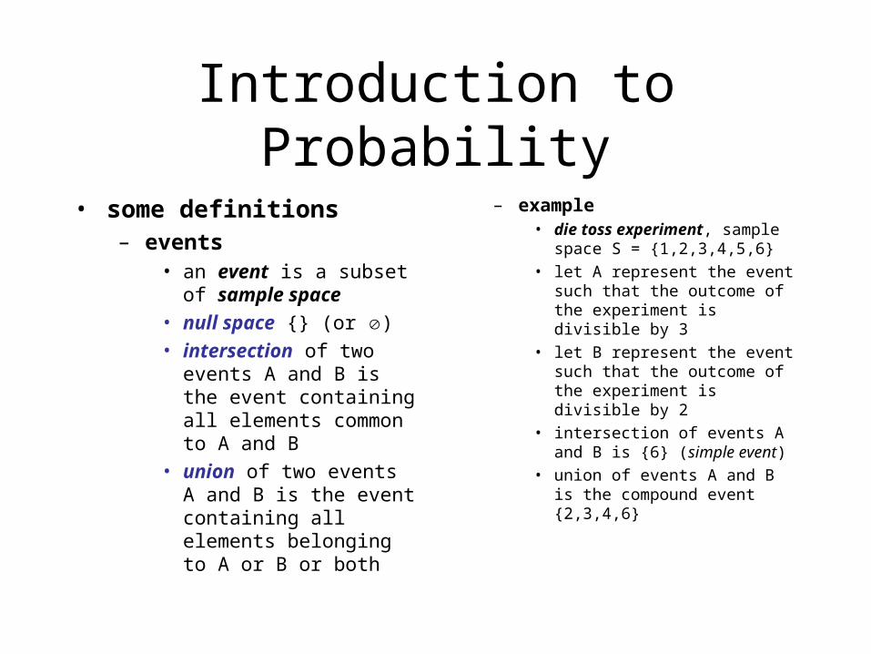
• some definitions– events
• an event is a subset of sample space
• null space {} (or )• intersection of two events
A and B is the event containing all elements common to A and B
• union of two events A and B is the event containing all elements belonging to A or B or both
– example• die toss experiment, sample
space S = {1,2,3,4,5,6}
• let A represent the event such that the outcome of the experiment is divisible by 3
• let B represent the event such that the outcome of the experiment is divisible by 2
• intersection of events A and B is {6} (simple event)
• union of events A and B is the compound event {2,3,4,6}

Introduction to Probability
• some definitions– rule of counting
• suppose operation oi can be performed in ni ways, a sequence of k operations o1o2...ok can be performed in
n1 n2 ... nk ways QuickTime™ and a
TIFF (Uncompressed) decompressorare needed to see this picture.
– example• die toss experiment, 6
possible outcomes• two dice are thrown at the
same time• number of sample points in
sample space = 6 6 = 36

Introduction to Probability
• some definitions– permutations
• a permutation is an arrangement of all or part of a set of objects
• the number of permutations of n distinct objects is n!
• (n! is read as n factorial)
– Definition:• n! = n x (n-1) ... x 2 x 1
• n! = n x (n-1)!• 1!=1 • 0!=1
1st
2nd
3rd
3 ways
2 ways
1 way
– example• suppose there are 3 students:
adam, bill and carol• how many ways are there of
lining up the students? • Answer: 6• 3! permutations

Introduction to Probability
• some definitions– permutations
• a permutation is an arrangement of all or part of a set of objects
• the number of permutations of n distinct objects taken r at a time is n!/(n-r)!
QuickTime™ and aTIFF (Uncompressed) decompressor
are needed to see this picture.
– example• a first and a second prize raffle
ticket is drawn from a book of 425 tickets
• Total number of sample points = 425!/(425-2)!
• = 425!/423!• = 425 x 424 = 180,200
possibilities• instance of sample space
calculation

Introduction to Probability
• some definitions– combinations
• the number of combinations of n distinct objects taken r at a time is n!/(r!(n-r)!)
• combinations differ from permutations in that in the former case the selection is taken without regard for order
– example• given 5 linguists and 4
computer scientists
• what is the number of three-person committees that can be formed consisting of two linguists and one computer scientist?
• note: order does not matter here
• select 2 from 5:
• 5!/(2!3!) = (5 x 4)/2 = 10
• select 1 from 4:
• 4!(1!3!) = 4
• answer = 10 x 4 = 40 (rule of counting)

Introduction to Probability
• some definitions– probability
• probability are weights associated with sample points
• a sample point with relatively low weight is unlikely to occur
• a sample point with relatively high weight is likely to occur
• weights are in the range zero to 1
• sum of all the weights in the sample space must be 1
(see smoothing)
• probability of an event is the sum of all the weights for the sample points of the event
– example• unbiased coin tossed twice
• sample space = {hh, ht, th, tt} (h = heads, t = tails)
• coin is unbiased => each outcome in the sample space is equally likely
• weight = 0.25
(0.25 x 4 = 1)
• What is the probability that at least one head occurs?
• sample points/probability for the event: hh 0.25 th 0.25 ht 0.25
• Answer: 0.75 (sum of weights)

Introduction to Probability
• some definitions– probability
• probability are weights associated with sample points
• a sample point with relatively low weight is unlikely to occur
• a sample point with relatively high weight is likely to occur
• weights are in the range zero to 1
• sum of all the weights in the sample space must be 1
• probability of an event is the sum of all the weights for the sample points of the event
heads and tailstails
1/3 2/3
– example• a biased coin, twice as likely
to come up tails as heads, is tossed twice
• What is the probability that at least one head occurs?
• sample space = {hh, ht, th, tt} (h = heads, t = tails)
• sample points/probability for the event:
– ht 1/3 x 2/3 = 2/9– hh 1/3 x 1/3= 1/9– th 2/3 x 1/3 = 2/9– tt 2/3 x 2/3 = 4/9
• Answer: 0.56 (sum of weights in bold)
• cf. probability of event for the unbiased coin = 0.75
> 50% chanceor < 50% chance?

QuickTime™ and aTIFF (Uncompressed) decompressor
are needed to see this picture.
S
Introduction to Probability
• some definitions– probability
• let p(A) and p(B) be the probability of events A and B, respectively.
• additive rule: p(A B) = p(A) + p(B) - p(A B)
• if A and B are mutually exclusive events: p(A B) = p(A) + p(B)
– since p(A B) = p() = 0
A B
– example• suppose probability of a student
getting an A in linguistics is 2/3 ( 0.66)
• suppose probability of a student getting an A in computer science is 4/9 ( 0.44)
• suppose probability of a student getting at least one A is 4/5 (= 0.8)
• What is the probability a student will get an A in both?
• p(A B) = p(A) + p(B) - p(A B)
• 4/5 = 2/3 + 4/9 - p(A B)
• p(A B) = 2/3 + 4/9 - 4/5 = 14/45 0.31

QuickTime™ and aTIFF (Uncompressed) decompressor
are needed to see this picture.
S
Introduction to Probability
• some definitions– conditional probability
• let A and B be events• p(B|A) = the probability of event B occurring given event A occurs• definition: p(B|A) = p(A B) / p(A) provided p(A)>0
– used an awful lot in language processing• (context-independent)• probability of a word occurring in a corpus
• (context-dependent)• probability of a word occurring given
the previous word

Entropy
• concept of uncertainty– example
• biased coin– 0.8 heads
– 0.2 tails
• unbiased coin– 0.5 heads
– 0.5 tails
QuickTime™ and aTIFF (Uncompressed) decompressorare needed to see this picture.
€
− pi lg pi
i=1
r
∑QuickTime™ and a
TIFF (Uncompressed) decompressorare needed to see this picture.
log conversionformula:
lg = log2
coin tossuncertainty vs.probability
• uncertainty measure (Shannon)– also mentioned a lot in corpus
statistics
• r =2, pi = probability the event is i
– biased coin• -0.8 * lg 0.8 + -0.2 * lg 0.2 = 0.258 +
0.464= 0.722
– unbiased coin: • - 2* 0.5 * lg 0.5 = 1
– it’s a measure of the sample space as a whole
uncertainty
50-50

Entropy
• uncertainty measure (Shannon)– given a random variable x
• r =2, pi = probability the event is i
– biased coin: 0.722, unbiased coin: 1
– entropy = H(x) = Shannon uncertainty
• perplexity– a measure of branching factor– 2H
– biased coin: 20.722 = 0.52– unbiased coin: 21= 2
€
− pi lg pi
i=1
r
∑
QuickTime™ and aTIFF (Uncompressed) decompressorare needed to see this picture.

Next Time
today we have seen fundamental concepts so far
• next– apply probability theory to language– Bayes’ Rule– N-grams– Peirera’s Experiment with “Colorless green ideas
sleep furiously”