Linear Theory of a Dual-Spin Projectile in Atmospheric Flight

by Mark F. Costello and Allen A. Peterson

Approved for public release, distribution is unlimited.

20000324 053

.

The fmdings in this report are not to be construed as an official Department of the Axmy position unless so designated by other authorized documents.

Citation of manufacturer’s or trade names does not constitute an official endorsement or approval of the use thereof.

Destroy this report wRen it is no longer ne43de4l. Do not return it to the originator.

Army Research Laboratory Aberdeen Proving Ground, h4D 2 1005-5066

ARL-CR-448 February 2000

Linear Theory of a Dual-Spin Projectile in Atmospheric Flight

Mark F. Costello and Allen A. Peterson Weapons and Materials Research Directorate, ARL

.

.

Abstract

The equations of motion for a dual-spin projectile in atmospheric flight are developed and subsequently utilized to solve for angle of attack and swerving dynamics. A combination hydrodynamic and roller bearing couples forward and aft body roll motions. Using a modified projectile linear theory developed for this configuration, it is sRown that the dynamic stability factor, S,, and the gyroscopic stability factor, S,, are altered compared to a similar rigid projectile, due to new epicyclic fast and slow arm equations. Swerving dynamics including aerodynamic jump are studied using the linear theory.

.

ii

Table of Contents

1.

2,

3.

4.

5.

6.

7.

8.

9.

List of Figures ..........................................................................................................

List of Symbols ........................................................................................................

Hntroduction .............................................................................................................

Dual-Spin Projectile Dynamic Model ....................................................................

Dual-Spin Projectile Linear Theory ......................................................................

Epicyclic Modes of Oscillation ...............................................................................

Dual-Spin Projectile Stability .................................................................................

Epicyclic Pitching and Yawing Motion .................................................................

Dual-Spin Projectile Swerve ...................................................................................

Concllusions ..............................................................................................................

References ................................................................................................................

Appendix: Rotation Dynamic Equations .............................................................

Distribution List ......................................................................................................

Report Documentation Page ..................................................................................

m

v

vii

1

2

5

10

14

22

24

26

29

31

41

47

.

l

. . . 111

&TENTIONALLY LEFT BLANK.

.

l

iv

List of Figures

. Figure

. I. Dual-Spin Projectile Schematic ................................................................................

2. Dual-Spin Projectile Geometry .................................................................................

3. Inertia Weighted Average Spin Rate vs. Roll Inertia Ratio ......................................

4. Gyroscopic Stability Factor, Sc, vs. Inertia Weighted Average Spin Rate ...............

5. Gyroscopic Spin Ratio vs. Gamma Dual Spin ..........................................................

6 Gyroscopic Stability Ratio vs. Differential Spin Ratio .............................................

7, Delta Ratio vs. Magnus Ratio ...................................................................................

8. Delta Ratio vs. Differential Spin Ratio .....................................................................

PaRe

1

6

16

16

19

19

20

20

INTENTIONALLY LEFT BLANK.

vi

List of Symbols

X,Y,Z

PF

PA

x,y,z

L, ,M, ,N,

LA,&,&

mF

mA

m

IF

Position vector components of the composite center of mass expressed in the inertial reference frame.

Euler pitch, and yaw angles.

Euler roll angle of the forward body.

Euler roll angle of the aft body.

Translation velocity components of the composite center of mass resolved in the fixed plane reference frame.

Roll axis component of the angular velocity vector of the forward body expressed in the fixed plane reference frame.

Roll axis component of the angular velocity vector of the aft body expressed in the fixed plane reference frame.

Components of the angular velocity vector of both the forward and aft bodies expressed in the fixed plane reference frame.

Total external force components on the composite body expressed in the fixed plane reference frame.

External moment components on the forward body expressed in the fixed plane reference frame.

External moment components on the aft body expressed in the fixed plane reference frame.

Forward body mass.

Aft body mass.

Total projectile mass.

Mass moment of inertia matrix of the forward body with respect to the forward body reference frame.

vii

I

D

ci

4,

a

B

V

TF

T4

G

r,,r,,r,

i:

R,,R,&

Mass moment of inertia matrix of the aft body with respect to the aft body reference frame. .

Effective inertia matrix.

Projectile characteristic length.

Various projectile aerodynamic coefficients.

Dynamic pressure at the projectile mass center.

Longitudinal aerodynamic angle of attack.

Lateral aerodynamic angle of attack.

Magnitude of mass center velocity.

Transformation matrix from the fixed plane reference frame to the forward

body reference frame.

Transformation matrix from the fixed plane reference frame to the aft body reference frame.

Fixed plane unit vectors.

Viscous damping coefficient for hydrodynamic bearing.

Friction coefficient for roller bearing.

Fixed plane components of vector from composite center of mass to forward

body mass center.

Fixed plane components of vector from composite center of mass to aft body

mass center.

Vector from composite center of mass to central bearing.

Fixed plane components of vector from forward body mass center to forward

body center of pressure.

. . . Vlll

&J&A, Fixed plane components of vector from aft body mass center to aft body

center of pressure.

Rmf,,Rmf,,Rmfi Fixed plane components of vector from forward body mass center to forward

body Magnus center of pressure.

Rm, , Rm, , Rm, Fixed plane components of vector from aft body mass center to aft body

Magnus center of pressure.

ix

.

WNTIONALLY LEFT BLANK.

X

1. Introduction

Compared to conventional munitions, the design of smart munitions involves more design

requirements stemming from the addition of sensors and control mechanisms. The addition of

these components must seek to minimize the weight and space impact on the overall projectile

design so that desired target effects can still be achieved with the weapon. The inherent design

conflict between standard projectile design considerations and new requirements imposed by

sensors and control mechanisms has led designers to consider more complex geometric

configurations. One such configuration is the dual-spin projectile. This projectile configuration

is composed of forward and aft components. The forward and aft components are connected

through a bearing, which allows the forward and aft portions of the projectile to spin at different

rates. Figure 1 shows a schematic of this projectile configuration.

Figure 1. Dual-Spin Projectile Schematic.

Dual-spin spacecraft dynamics have been extensively studied in the literature. For example,

Likins [l] studied the motion of a dual-spin spacecraft and conditions for stability were

established. Later, Cloutier [2] obtained an analytical criterion for infinitesimal stability. Along

these lines, Mingori [3] as well as Fang [4] considered energy dissipation. Hall and Rand [5]

considered spinup dynamics, and resonances occurring during despin were studied by Or [6]. In

the latter, the linear equations governing the resonance dynamics were found to depend on

nondimensional parameters related to dynamic unbalance, asymmetry, and the time duration for

resonance growth. Other work investigating asymmetric mass properties is due to Co&ran, Shu,

and Rew [7] as well as Tsuchiya [8] and Yang [9]. Viderman, Rimrott, and Cleghom [lo]

developed a dynamic model of a dual-spin spacecraft with a flexible platform. Stability was

investigated using Floquet theory. Stabb and S&lack [ll] investigated pointing accuracy of a

dual-spin spacecraft using the Krylov-Bogoliubov-Mitropolsky perturbation method.

For projectile flight in the atmosphere, aerodynamic forces and moments play a dominant

role in the dynamic characteristics. These effects have obviously not been considered in the

dual-spin spacecraft efforts described previously. However, Smith, Smith, and Topliffe [12]

considered the dynamics of a spin-stabilized artillery projectile modified to accommodate

controllable canards mounted to the projectile by a bearing aligned with the spin axis. This work

focused on the use of actively controlled canards to reduce miss distance. Both the forward and

aft bodies were mass balanced and a hydrodynamic bearing coupled forward and aft body rolling

motion

The dual-spin projectile model developed here permits nonsymmetric forward and aft body

components and allows a combination of hydrodynamic and roller bearing roll coupling between

the forward and aft bodies. By applying the linear theory for a rigid projectile in atmospheric

flight, a dual-spin projectile linear theory is developed. Expressions for the gyroscopic and

dynamic stability factor are developed and compared to the rigid projectile case. The swerving

motion of this configuration is also considered.

2. Dual-Spin Projectile Dynamic Model

The mathematical model describing the motion of the dual-spin projectile allows for three

translation and four rotation rigid body degrees of freedom (DOF). The translation degrees of

freedom are the three components of the mass center position vector. The rotation degrees of

freedom are the Euler yaw and pitch angles as well as the forward body roll and aft body roll

angles. The ground surface is used as an inertial reference frame [13].

Development of the kinematic and dynamic equations of motion is aided by the use of an

intermediate reference frame. The sequence of rotations from the inertial frame to the forward

and aft bodies consists of a set of body fixed rotations that are ordered: yaw, pitch, and

2

forward/aft body roll. The fixed plane reference frame is defined as the intermediate frame

before roll rotation. The fixed plane frame is convenient because both the forward and aft bodies

share this frame before roll rotation.

Equations l-4 represent the translation and rotation kinematic and dynamic equations of

motion for a dual-spin projectile. Both sets of dynamic equations are expressed in the fixed

plane reference frame.

(1)

(3)

A derivation of equation 4 is provided in the Appendix.

Loads on the composite projectile body are due to weight and aerodynamic forces acting on

both the forward and aft bodies. Equations 5 and 6 provide expressions for the forward body

weight and aerodynamic forces.

I I -se =m,g 0

ce (5)

Linear Magnus forces acting on the forward body are formulated separately in equation 7. These

forces act at the Magnus force center of pressure, which is different from the center of pressure

of the steady aerodynamic forces.

The longitudinal and lateral aerodynamic angles of attack used in equations 6 and 7 are

(7)

computed using equation 8.

I B = tan -1 (8)

(9)

4

Expressions for the aft body forces take on the same form. Aerodynamic coefficients in

equations 6 and 7 depend on the local Mach number at the projectile mass center. They are

computed using linear interpolation from a table of data.

The right-hand side of the rotation kinetic equations contains the externally applied moments

on both the forward and aft bodies. These equations contain contributions from steady and

unsteady aerodynamics. The steady aerodynamic moments are computed for each individual

body with a cross product between the steady body aerodynamic force vector and the distance

vector from the center of gravity to the center of pressure. Magnus moments on each body are

computed in a similar way, with a cross product between the Magnus force vector and the

distance vector from the center of gravity to the Magnus center of pressure. Figure 2 shows the

relative locations of the forward, aft, and composite body centers of gravity and the forward and

aft body centers of pressure. The unsteady body aerodynamic moments provide a damping

source for projectile angular motion and are given for the forward body by equation 10.

=&D (10)

Air density is computed using the center of gravity position of the projectile in concert with the

standard atmosphere [ 141.

3. Dual-Spin Projectile Linear Theory

The equations of motion listed previously are highly nonlinear and not amenable to a

closed-form analytic solution. Linear theory for symmetric rigid projectiles introduces a

Composite Body

Couples bodies

Figure 2. Dual-Spin Projectile Geometry.

sequence of assumptions, which yield a tractable set of linear differential equations of motion

that can be solved in closed form. These equations form the basis of classic projectile stability

theory. The same set of assumptions can be used to establish a linear theory for dual-spin

projectiles in atmospheric flight.

A) Change of variables from fixed plane, station line velocity, u, to total velocity, V. Equations

11 and 12 relate V and u and their derivatives.

v=Ju2+v2+w2

vi= uli+v++ti

V (12)

B) Change of variables from time, t, to dimensionless arc length, s. The dimensionless arc

length, as defined by Murphy [ 151 is given in equation 13 and has units of calibers of travel.

2. j, .& s Do

(11)

(13)

Equations 14 and 15 relate time and arc length derivatives of a given quantity c . Dotted

terms refer to time derivatives, and primed terms denote arc length derivatives.

(14)

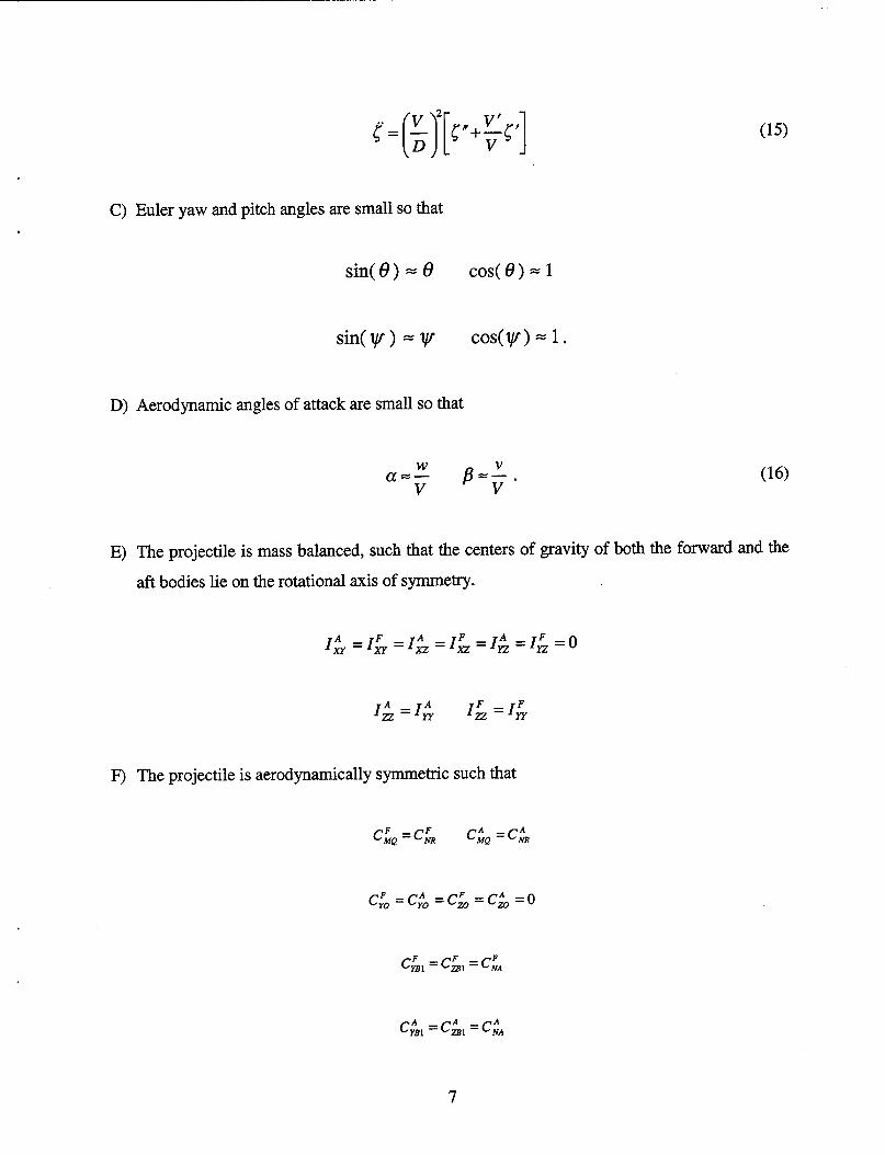
C) Euler yaw and pitch angles are small so that

sin(e)=8

swv) =Y

D) Aerodynamic angles of attack are small so that

cos(8)=1

cos(yr)=l.

E) The projectile is mass balanced, such that the centers of gravity of both the forward and the

aft bodies lie on the rotational axis of symmetry.

F) The projectile is aerodynamically symmetric such that

c NR F =p MQ ctQ =c&

CF cc* =cF =cA =o YO YO W W

CF cc” =cF YE1 ZBl NA

C A, = CA, = c&

7

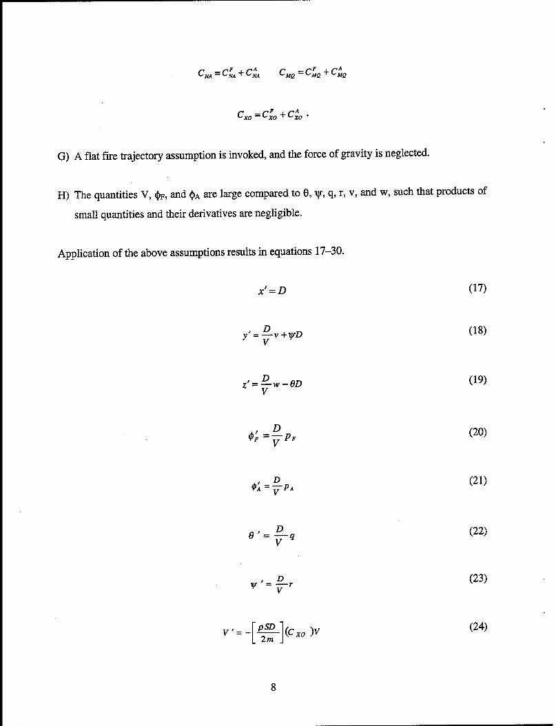
G) A flat fire trajectory assumption is invoked, and the force of gravity is neglected.

FI) The quantities V, @, and $A are large compared to 8, v, q, r9 v, and w, such that products of

small quantities and their derivatives are negligible.

Application of the above assumptions results in equations 17-30.

y* = +v +lyD

Z p- +V-0D

(18)

(191

(27)

(28)

Equations 17-30 are linear, except for the total velocity, V, which is retained in several of the

equations. Using the assumption that V changes very slowly with respect to the other variables,

it is considered to be constant when it appears as a coefficient. With this assumption, the total

velocity, the angle of attack dynamics, and the roll dynamics all become uncoupled, linear-time

invariant equations of motion. The Magnus force in equations 25 and 26 is typically regarded as

small in comparison to the other aerodynamic forces and is shown only for completeness. In

further manipulation of the equations, all Magnus forces will be dropped. Magnus moments will

9

be retained, however, due to the magnitude amplification resulting from the cross product

between Magnus force and its respective moment arm.

4. Epicyclic Modes of Oscillation

Equations 17-23 state that the fixed plane is mapped directly onto the inertial reference

frame for the given assumptions. Equations 27 and 28 show that a roller bearing model requires

knowledge of the zero-yaw drag on the forward and aft body separately. Also notice that the

Magnus moments appear separately in equations 29 and 30. The equations for total velocity and

the fore and aft spin rates have become completely decoupled from the angle of attack dynamics.

It is a useful result to begin by studying equation 24, which represents the total velocity, V, of

the projectile. Equation 24 is separable, and it is elementary to obtain the solution as downrange

exponential decay.

V(s) = V,e -9X0 t j (31)

After extracting the decoupled equations for total velocity and fore and aft spin rates, there

are only four equations remaining to examine. These equations describe fixed plane expressions

for translational and rotational velocities v, w, q, and r. The angle of attack dynamics are driven

directly by these four equations because the aerodynamic angles of attack depend on v and w by

definition.

Using equation 31 and the definition for small angles of attack given in equation 16, the

following two relations can be written.

a(s) = 4s) _ w(s) e[E+ VW v,

(32)

10

v(s) VW (*) B(s)=,0=y 0

(33)

The translational and rotation velocities are described in a compact form as shown in equation

34,

V'

W' = ii II_ -A

q’ E rl -C

D

where

0

-A C

D B

D

0

D

E

F

A=

ZA =I& -tmfrfi2 +ZA +m,r,‘.

(34)

(35)

(36)

(37)

(38)

W)

(41)

11

Eigenvalues of equation 34 provide the fast and slow epicyclic modes of oscillation for v, w, q,

and r. The four roots of the characteristic equation are displayed below.

(IT-A)+iFzt (E-A)2 -F2 +4(AE+C)+2iF 11 s= (42)

(E-A)-iF+ (E-A)2 -F2+4(A.E+C)-2% 11 Linear combinations of the previous equations lead to equation 43.

In line with rigid body, six degrees of freedom projectile stability analysis, two more

simplifications based on size are introduced. First, neglect the product of the damping factors

:

(E-4 iF

-AE-C

-i(AF +B)

h +4

i 1 4% +Q>s) = aFas -<~,a,

-I

(43)

compared to the product of the damped natural frequencies. Secondly, neglect the product of A

and E, because multiples of the relative density factor are small compared with the magnitudes of

other terms. A solution may now be obtained for both the fast and the slow damping factors and

turning rates for the translational and rotational velocities.

(45)

a?, +-m-c] (47)

Before making conclusions about the stability of the angle of attack dynamics, the damping

factors and the damped natural frequencies have to be calculated for a and fl rather than v and w.

These new damping factors will account for the fact that v, w, and V all decay downrange.

Whether a and p are stable depends on which quantities decay fastest. Two new damping

factors are introduced based on equations 32 and 33.

I (2AF+2+,F +2B]

A-2*&-E 2m

(48)

(49)

The fast and slow turning rates represent the imaginary parts of the complex eigenvalues. These

will remain unchanged for a and p, because division by V(s) in equations 32 and 33 only affects

the real parts of the eigenvalues. If either @r or @s is complex, there will be a positive real part

in one of the four eigenvalues. To avoid complex turning rates, the term under the radical in

equations 45 and 47 must be greater than zero, introducing the idea of the gyroscopic stability

factor So.

F2 s, E-

4.c’ (50)

13

Furthermore, the dynamic stability factor is defined by equation 5 1.

SD =

jZAF+2EC,FtZB) -E

(51)

The fast mode damping factor, Ai , must be negative for stable flight. To ensure stability, the

following two conditions must be satisfied.

r ,4-2+,-E)>O (52) \ zm /

+< &(2-S,) G

The results shown in equations 50-53 are very similar

(53)

to conventional rigid body projectile

analysis. Hence, dual-spin projectile stability analysis can be approached in essentially the same

manner that rigid projectiles are analyzed. Differences in stability characteristics arise from the

coeffkients F and B. The coefficient F contains terms with forward and aft body roll rate and

roll inertia appearing separately. Magnus moments also appear separated in the coeffkient B,

due to their dependence on the fore and aft roll rates.

5. Dual-Spin Projectile Stability

The gyroscopic and dynamic stability factors can be reexpressed as shown in equations 54

and 55.

4

s _ <G a’ G- 21; M

(54)

where

pc = (PF +YDSPA)

(l + YDS )

YDS I& =- G

G =(IL +I&)=I&(l+yDs)

M =pwc~

p* = (PF + PDSPA) (l + PDS )

(55)

(56)

(57)

(58)

(5%

(60)

(61)

(62)

The inertia weighted average spin rate for the composite body, j! , is biased to the spin rate

of the body with the largest roll inertia component. The Magnus weighted average spin rate, p* ,

behaves in precisely the same manner as F ; however, it is biased toward the body with the

largest Magnus moment. A plot of jj vs. roll inertia ratio, 70,~ , and p* vs. Magnus ratio,

15

pDs , is shown in Figure 3. When yDs = 0, F is equal to pF , while as YLS + co , F

approaches pA . Similar relations ‘hold between puos and p* . Gyroscopic stability factor Vs.

inertia weighted average spin rate is plotted as Figure 4 for various values of composite inertia

and external moments.

,Y DS I

0 0°1.‘,5

Figure 3. Inertia Weighted Average Spin Rate vs. Roil Inertia Ratio.

Gyroscopimlly Stable

Gymscoplcally Unstable

b

Figure 4. Gyroscopic Stability Factor, SG, vs. Inertia Weighted Average Spin Rate.

16

It is interesting to expand equation 55 and examine the results. The dynamic stability factor

can be broken into two parts. The first part, shown in equation 64 represents a stability factor

offset that is independent of whether the system is a rigid or dual-spin projectile. Equation 65

shows the second part, which does vary with respect to the rigid projectile case depending on the

Magnus moment coefficients and spin rates. This portion of the total stability factor is directly

proportional to the total Magnus moment acting about the composite center of mass and can be

considered as a dynamic stability enhancement factor.

S,=H+A,, ,

where

i

dh.JA -C,) H = (c, -2c, ,-[y+J

A DS =

GTp’ .

(63)

(64)

(65)

It is also informative to compare the dual-spin projectile stability factors to the conventional

rigid projectile results. To do this, define F and Ap as the average spin rate and the spin rate

difference, respectively. Thus,

PF =jF+Ap p,=jT-Ap.

The spin rate of an equivalent rigid projectile is p. The ratio of the dual-spin gyroscopic

stability factor to the rigid projectile gyroscopic stability factor is shown as equation 66.

17

Equation 67 shows the ratio of dynamic stability enhancement factors between the dual-spin case

and the rigid projectile case. These two relations are again of very similar form.

(66)

(67)

Figures 5 and 6 represent equation 66 as a function of the roll inertia ratio and the differential

spin ratio. When the gyroscopic stability factor ratio is greater than one, dual-spin gyroscopic

stability is enhanced compared to the rigid projectile with a roll rate of p. It can be shown that

the differential spin ratio is positive when the forward body is spinning faster than the aft, and

negative when the reverse is true. The curves can also be grouped by the roll inertia ratio. When

y DS is less than one, the forward body has more roll inertia. The aft inertia is larger when

y DS is greater than one. Based on the values of the differential spin ratio and roll inertia ratio,

Figures 5 and 6 can be viewedin separate quadrants. When both ratios favor one of the bodies,

gyroscopic stability is enhanced. When the ratios favor opposite bodies, the stability factor is

diminished. Note that the gyroscopic stability ratio can never become negative because the

values compared are squared. Also note that in physical systems, the differential spin ratio must

be zero when y DS goes to zero or infinity.

Figures 7 and 8 represent equation 66 as a function of the Magnus ratio and the differential

spin ratio. When the magnitude of the dynamic enhancement ratio is greater than one, both the

total Magnus moment and the dynamic stability enhancement factor are larger than the rigid

projectile case. This can result from several physical situations, which are represented by again

considering the graphs in sections.

18

.

2.5

1

1.5

AP -= F O

3

2.5

2

.;

2 1.5

$

1

0.5

0.:5 0.5 0.75 1 l.25 1.5 1.75 2

YOS

Figure 5. Gyroscopic Spin Ratio vs. Gamma Dual Spin.

-1.5 -1 -0.5 0 0.5 1 1.5 7.

Delu p I Avcrrge p

Figure 6. Gyroscopic Stability Ratio vs. Differential Spin Ratio.

When the Magnus ratio is between negative and pdsitive one, the Magnus moment

coefficient is larger for the forward body than for the aft. When the Magnus ratio is outside of

19

0.5 1.5 t

4.5 -1 -0.5 A

Figure 7. Delta Ratio vs. Magnus Ratio.

AP y=0

-1 1.5

Figure 8. Delta Ratio vs. Differential Spin Ratio.

these boundaries, the aft body has a larger Magnus coeffkient. Negative Magnus ratios indicate

that the aft Magnus center of pressure is rearward of the composite body mass center. Positive

20

values of the differential spin ratio again indicate that the forward body is spinning faster than

the aft. With this in mind, Figures 7 and 8 can be viewed where both ratios favor one body, or

where they favor opposite bodies. For the first case, the total Magnus moment applied to the

dual-spin projectile is larger than that of the rigid case. The opposite is true when the ratios

favor opposite bodies.

Some special values of Magnus ratio must also be considered. Magnus ratio equal to one

indicates the Magnus coefficients are equivalent or, physically, that the centers of pressure and

force coefficients are equivalent. In this situation, the dual-spin case will have the same Magnus

moment as the rigid case because p* and p do not differ. When Magnus ratio is equal to

negative one, the Magnus coeffkients are equal and opposite. For the rigid case where the

bodies spin together, the Magnus moment will go to zero and drive the enhancement ratio to

infinity.

Dual-spin projectile stability results must match the standard rigid projectile stability results

in two situations. First, either of the bodies may be neglected by setting their mass and inertia

properties and force coeffkients to zero. In this case, the inertia properties of the total body

reduce to those of the remaining body and the roll inertia ratio becomes either 0 or 00, depending

on which body remains. Using the same logic, p becomes either pF or pA. Also, the moments

considered, including Magnus, are only those applied to the remaining body. With these

assumptions, the rigid body stability results are obtained.

The second case to consider is when the forward and aft bodies spin together. For this case,

both the inertia weighted average spin rate and the Magnus weighted average spin rate are equal

to both the front and rear spin rates, since the projectile bodies are spinning together. This result

is true regardless of the roll inertia ratio. The inertia properties are for the total body, as are the

applied moments. Again, the rigid body stability results are obtained.

21

6. Epicyclic Pitching and Yawing Motion

Equation 34 has been used to solve for the dynamic modes of projectile pitching and yawing

motion along its flight path. To complete the analytical solution, the two complex conjugate

pairs of modes in equation 41 must be used to evaluate the system mode shapes. Solutions will

be obtained for v and w, and these will be used to evaluate a and /? .

Mode shapes for equation 34 are displayed in the matrix V, described by equations 68-72

using the familiar coeffkients. By applying the relations in equation 43, equations 68-72 can be

expressed completely in terms of the coefficient A, and the fast and slow mode damping factors

and turning rates.

where

i i -i -i

K+l&. K-;& 1 1

PI= R+df R-G

i(Z)&) i(?&) i(R?f) i(RtDfi)

20 - 20 20 20

, (68)

K =(E-A)+2A+iF =(;1, +il,)+M+i(Q>. +@,) (69)

Q =(E-A)2 +4AE+4C-F2 +2i(F(E-A)+Z@F+B))=((& -&)+i(@,, -@,)y (70)

R=(E-A)+2A-iF=(&+il,)+2A-i&+@>,) (71)

S=(E-A)2+4AE+4C-F2 -2i(F(E-A)+2(AF+B))=((& -Q-i@‘, -@,))“. (72)

Recognizing that the turning rates are between one and two orders of magnitude greater than

the damping factors, equation 68 can be simplified to equation 73.

22

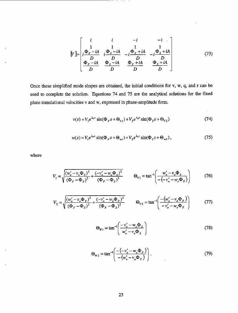
I- i i -i -i 1 F-J= i a,‘-iA I D _i@L +iA . QS1-iA

CD,? iA Q>, -iA @,:A

(73)

Once these simplified mode shapes are obtained, the initial conditions for v, w, q, and r can be

used to complete the solution. Equations 74 and 75 are the analytical solutions for the fixed

plane translational velocities v and w, expressed in phase-amplitude form.

v(s) = V1eAFS sin(Qi.s+0,,)+V,e4’sin(~,s+0,,) (74)

w(s) =V1eAFS sil@Q + O,,) +vp sin(<f,,s+ O,,) , (75)

where

(78)

(79)

23

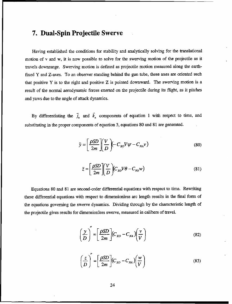
7. Dual-Spin Projectile Swerve

Having established the conditions for stability and analytically solving for the translational

motion of v and w, it is now possible to solve for the swerving motion of the projectile as it

travels downrange. Swerving motion is defined as projectile motion measured along the earth-

fixed Y and Z-axes. To an observer standing behind the gun tube, these axes are oriented such

that positive Y is to the right and positive Z is pointed downward. The swerving motion is a

result of the normal aerodynamic forces exerted on the projectile during its flight, as it pitches

and yaws due to the angle of attack dynamics.

By differentiating the jn and &, components of equation 1 with respect to time, and

substituting in the proper components of equation 3, equations 80 and 81 are generated.

f= pso [ 2m

(81)

Equations 80 and 81 are second-order differential equations with respect to time. Rewriting

these differential equations with respect to dimensionless arc length results in the final form of

the equations governing the swerve dynamics. Dividing through by the characteristic length of

the projectile gives results for dimensionless swerve, measured in calibers of travel.

24

(82)

(83)

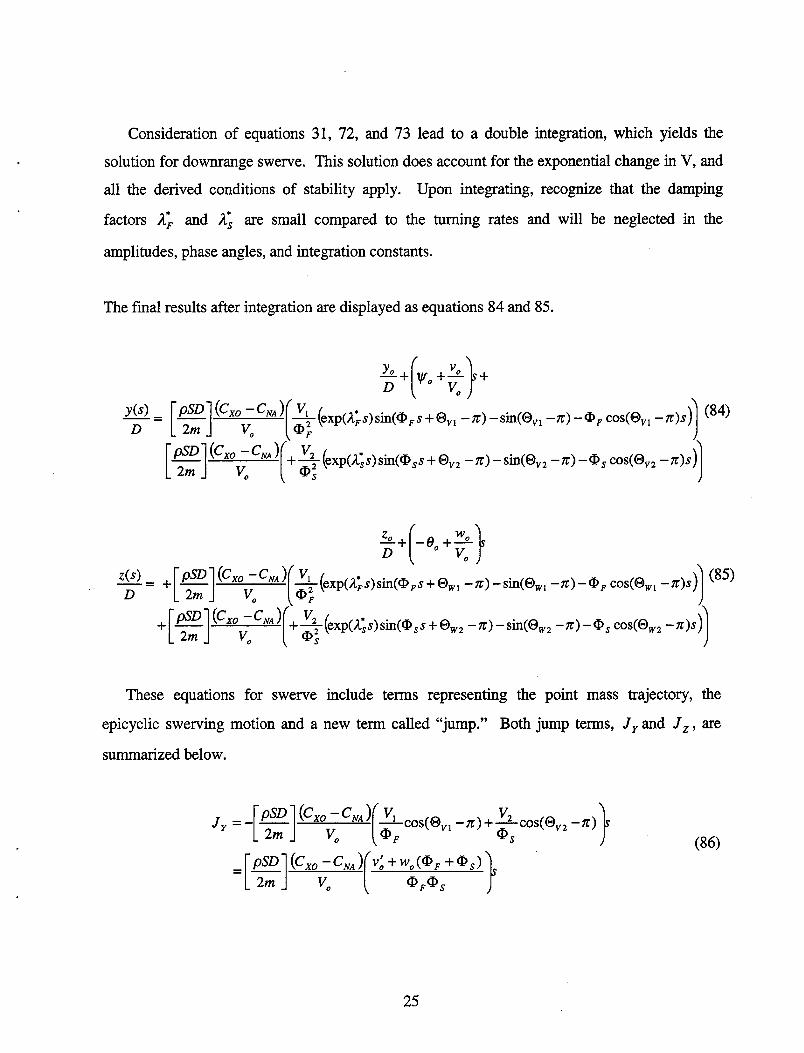
Consideration of equations 3 1, 72, and 73 lead to a double integration, which yields the

solution for downrange swerve. This solution does account for the exponential change in V, and

all the derived conditions of stability apply. Upon integrating, recognize that the damping

factors A> and Ai are small compared to the turning rates and will be neglected in the

amplitudes, phase angles, and integration constants.

The fmal results after integration are displayed as equations 84 and 85.

These equations for swerve include terms representing the point mass trajectory, the

epicyclic swerving motion and a new term called “jump.” Both jump terms, J, and J, , are

summarized below.

25

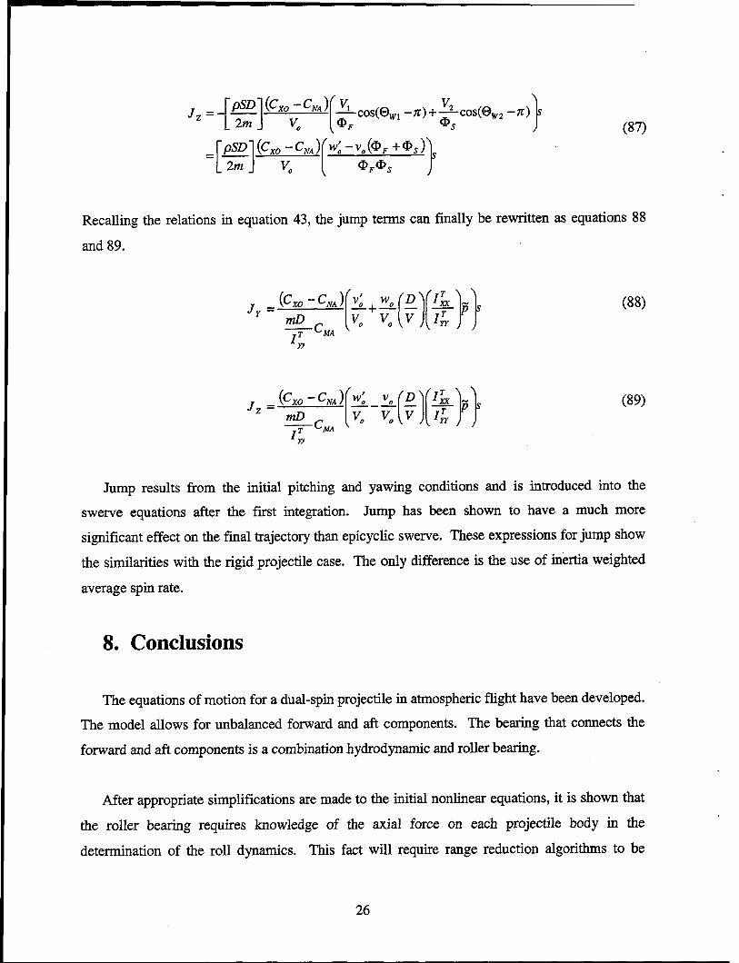
(87)

Recalling the relations in equation 43, the jump terms can finally be rewritten as equations 88

and 89.

(89)

Jump results from the initial pitching and yawing conditions and is introduced into the

swerve equations after the first integration. Jump has been shown to have a much more

significant effect on the final trajectory than epicyclic swerve. These expressions for jump show

the similarities with the rigid projectile case. The only difference is the use of inertia weighted

average spin rate.

8. Conclusions

The equations of motion for a dual-spin projectile in atmospheric flight have been developed.

The model allows for unbalanced forward and aft components. The bearing that connects the

forward and aft components is a combination hydrodynamic and roller bearing.

After appropriate simplifications are made to the initial nonlinear equations, it is shown that

the roller bearing requires knowledge of the axial force on each projectile body in the

determination of the roll dynamics. This fact will require range reduction algorithms to be

26

modified to estimate the axial force on both components from roll angle and roll data. The

hydrodynamic bearing does not have this complication because the reaction moment on a

hydrodynamic bearing is a function of the roll rate difference only.

It is possible to analyze the stability of a dual-spin projectile using a methodology similar to

rigid body projectile stability analysis. The gyroscopic stability factor, So, is different from the

conventional rigid projectile results. It depends on the spin rates of both bodies as well as their

individual roll inertias. However, it is possible to define the inertia weighted average spin rate,

F, which is essentially an equivalent spin rate such that the form of the gyroscopic stability

factor is the

both bodies

results.

same as the rigid projectile case. When either the fore or aft body is removed, or

spin together, the stability results reduce to the standard rigid projectile stability

The dynamic stability factor is also different from the conventional rigid projectile results.

To emulate the standard results, a Magnus weighted average spin rate, p* is introduced. The

dynamic stability factor can be shown to match the rigid case under the same two conditions that

were checked for the gyroscopic stability factor. The dynamic stability enhancement ratio

depends on the differential spin ratio and the Magnus ratio, which may both become negative.

27

INTENTIONALLY LEFT BLANK.

28

1.

2.

3.

4.

5.

6.

7.

8.

9.

10.

11.

9. References

L&ins, P. W. “Attitude Stability Criteria for Dual-Spin Spacecraft.” Journal of Spacecraf and Rockets, vol. 4, pp. 1638-1643, 1967.

Cloutier, G. J. “Stable Rotation States of Dual-Spin Spacecraft.” Journal of Spacecraft and Rockets, vol. 5, pp. 490-492, 1968.

Mingori, D. L. “Effects of Energy Dissipation on the Attitude Stability of Dual Spin Satellites.” AZAA Journal, vol. 7, pp. 20-27, 1969.

Fang, B. T. “Energy Considerations for Attitude Stability of Dual-Spin Spacecraft.” Journal of Spacecraft and Rockets, vol. 5, pp. 1241-1243,1968.

Hall, C. D., and R. H. Rand. “Spinup Dynamics of Axial Dual-Spin Spacecraft.” Journal of Guidance, Control, and Dynamics, vol. 17, pp. 30-37, 1994.

Or, A. C. “Resonances in the Despin Dynamics of Dual-Spin Spacecraft.” Journal of Guidance, Control, and Dynamics, vol. 14, pp. 321-329, 1991.

Co&ran, J. E., P. H. Shu, and S. D. Rew. “Attitude Motion of Asymmetric Dual-Spin Spacecraft.” Journal of Guidance, Control, and Dynamics, vol. 5, pp. 37-42, 1982.

Tsuchiya, K. “Attitude Behavior of a Dual-Spin Spacecraft Composed of Asymmetric Bodies.” Journal of Guidance, Control, and Dynamics, vol. 2, pp. 328-333, 1979.

Yang, H. X. “Method for Stability Analysis of Asymmetric Dual-Spin Spacecraft.” Journal of Guidance, Control, and Dynamics, vol. 12, pp. 123-125, 1989.

Viderman, Z., F. P. J. Rimrott, and W. L. Cleghom. “Stability of an Asymmetric Dual-Spin Spacecraft with Flexible Platform.” Journal of Guidance, Control, and Dynamics, vol. 14, pp. 751-760,199l.

Stabb, M. C., and A. L. S&lack. “Pointing Accuracy of a Dual-Spin Satellite Due to Torsional Appendage Vibrations.” Journal of Guidance, Control, and Dynamics, vol. 16, pp. 630-635,1991.

12.’ Smith, J. A., K. A. Smith, and R. Topliffe. “Feasibility Study for Application of Modular Guidance and Control Units to Existing ICM Projectiles.” Final Technical Report, Contractor Report ARLCD-CR-79001, U.S. Army Armament Research and Development Command, 1978.

13. Etkin, B. Dynamics of Atmospheric Flight. New York, NY: John Wiley and Sons, 1972.

29

14.

15.

Von Mises, R. Theory of Flight. New York, NY: Dover Publications Inc., 1959.

Murphy, C. H. “Free Flight Motion of Symmetric Missiles.” BRL Report No. 1216, U.S. Army Ballistic Research Laboratories, Aberdeen Proving Ground, MD, 1963.

30

Appendix:

Rotation Dynamic Equations

31

INTENTIONALLY LEFT BLANK.

32

The rotation kinetic differential equations are derived by splitting the two-body system at the

bearing connection point. A constraint force, F, , and a constraint moment, M’ C , couple the

forward and aft bodies. The translational dynamic equations for both bodies are given by

equations A-l and A-2.

mAa',,, = FA + Fc (A-1)

mFaFII =PF --& 64-2)

Key to the development of the rotation kinetic differential equations is the ability to solve for the

constraint forces and moments as a function of state variables and time derivatives of state

variables. An expression for the constraint force can be obtained by subtracting equation A-2

from equation A- 1.

mFmA mF mA

(A-3)

With the constraint force known, the rotational dynamic equations for the forward and aft bodies

can be developed. The constraint force contributes to the applied moments from a. cross product

between the constraint force vector and the position vectors from the individual centers of

gravity to the bearing. An additional constraint moment couples the forward and aft bodies due

to viscous or rolling friction in the bearing.

-&I =G,-ti,-p,xFc,

(A-4)

(A-5)

where

33

p, =JA-F (A-6)

p’, =FF -r . (A-7)

The acceleration of the mass center of the forward and aft bodies, a’,,, and ZAII, cm be

expressed in terms of the acceleration of the composite body mass center. After making this

substitution, the constraint force components in the fixed plane reference frame can be expressed

in the following manner.

1 F cx

GY (A-8)

&z

The constraint moment components in the fared plane reference frame acting on the forward

body about the forward body mass center, and resulting from the constraint force cross product

can be written in the following manner.

(A-9)

In a similar way, the components in the fixed plane reference frame of the moment of the

constraint force acting on the aft body about the aft body mass center can be written as shown in

equation A-l 0.

(A-10)

34

The rotation kinetic differential equations are both expressed in the fixed plane reference

frame. The equations are left general and allow for a fully populated inertia matrix and mass

unbalance. Equations A-8-A-10 are substituted into both sets of rotation kinetic equations for

the forward and aft bodies. At this point, both sets of equations still have unknown constraint

moments at the bearing connection point. To eliminate the bearing constraint moments in the

fixed plane j,, and in directions, the j,, and g,, components of the rotation kinetic equations for

the forward and aft bodies are added together to form two dynamic equations that are free of

constraint moments. In this way, the constraint moments at the bearing have been eliminated

analytically from the pitching and yaw dynamics.

To finish expressing the roll dynamic equations, however, an expression for the unknown

constraint moment must be formed. The moment transmitted across the bearing is modeled as a

combination hydrodynamic and roller bearing. The contribution from the hydrodynamic bearing

can be modeled as viscous damping’ and the constitutive relation governing the constraint

moment is given by equation A- 11.

The frictional moment at a roller bearing is proportional to the normal force acting on the

(A-l 1)

bearing. Normal force at the bearing of a split bodied projectile is directly related to the axial

aerodynamic coeffkients of the forward and aft bodies. The contribution to the constraint

moment from a roller bearing* is given by equation A-12. To remove the effects of either

bearing from the model, set the respective coefficient to zero.

M: = C,IF,, Isign(pF - PA) (A-12)

’ Close, C. M., and D. K. Frederick. Modeling and Analysis of Dynamic Systems. New York, NY: John Wiley and Sons, 1995.

2 Bolz, R. E., and G. L. Tuve. CRC Handbook of Tables for Applied Engineering Science. OH: CRC Press, 1973.

35

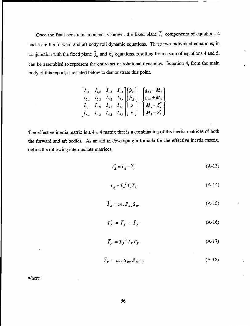
Once the final constraint moment is known, the fixed plane c components of equations 4

and 5 are the forward and aft body roll dynamic equations. These two individual equations, in

conjunction with the fixed plane jn and &, equations, resulting from a sum of equations 4 and 5,

can be assembled to represent the entire set of rotational dynamics. Equation 4, from the main

body of this report, is restated below to demonstrate this point.

The effective inertia matrix is a 4 x 4 matrix that is a combination of the inertia matrices of both

the forward and aft bodies. As an aid in developing a formula for the effective inertia matrix,

defme the following intermediate matrices.

I; =i, -TA

f-A = TATIATA

TA = mASRA S,

IJ =FF --TF

TF = TFTIFTF

rF =mFSRFSRF ,

where

36

(A-13)

(A-14)

(A-15)

(A-16)

(A-17)

(A-18)

(A-19)

(A-20)

(A-2 1)

(A-22)

Using equations A-13, A-16, A-11, and A-12, elements of the effective inertia matrix can now be

formed.

I 1.1 = ‘I;,,, + Mm,,,

I 1.2 = Mm,.,

I 1,4 = Ii,., + MFQ + M,,g

12.1 = M,,,

37

(A-23)

(A-24)

(A-25)

(A-26)

(A-27)

I 22 = I;., -&A,**

I 2.3 =I;., -“w.? -MAEi.2

I 2,4 =I;., -K4Al,s -MA%

I =‘Fz, 3.1 .

I 32 = It.1

I 3.3 = ‘K., + L.z

I3,4 = IX., + ‘;.1

I 4.2 = I;.*

(A-28)

(A-29)

(A-30)

(A-3 1)

(A-32)

(A-33)

(A-34)

(A-35)

(A-36)

I 4,3 = ‘;;,,, + ‘h., (A-37)

14.4 = ‘is., + ‘is,3 (A-38)

Two elements of the right-hand side vector of equation 4, from the main body of this report, are

given by equations A-39 and A-40.

gF, = ti 0 Ol[M, -S; -&,I (A-39)

38

The vectors 3: and 3; in equation 89, from the main body of this report, and equation A-l are

given by equations A-41 and A-42.

where

s, = [TATI,FA +TATSAIATA

PO

s; = FF - ITF

FF = bFT I& +TrTSFIFTF

L J

(A-41)

(A-42)

(A-43)

(A-44

(A-45)

(A-W

39

S [

0 --r 4

wF=

r 0 1

-PF

-qPF ’

s

Other unknown terms on the right-hand’side of equation A-4 include components of the vectors

&? and s* . These vectors are described below.

(A-47)

(A-W

NO. OF COPIES

2

ORGANIZATION

DEFENSE TECHNICAL JNFORMATJON CENTER DTIC DDA 8725 JOHN J IUNGMAN RD STE 0944 FT BELVOIR VA 22060-62 18

HQDA DAM0 FDQ D SCHMIDT 400 ARMY PENTAGON WASHINGTON DC 203 1 O-0460

GSD OUSD(A&T)/ODDDR&E(R) RJTREW THE PENTAGON WASHINGTON DC 20301-7100

DPTY CG FOR RDA US ARMY MATERIEL CMD AMCRDA 5001 EISENHOWER AVE ALEXANDRIA VA 22333-0001

INST FOR ADVNCD TCHNLGY THE UNIV OF TEXAS AT AUSTIN PO BOX 202797 AUSTIN TX 78720-2797

DARPA B KASPAR 3701 N FAIRFAX DR ARLINGTON VA 22203- 17 14

NAVAL SURFACE WARFARE CTR CODE B07 J PENNELLA 17320 DAHLGREN RD BLDG 1470 RM 1101 DAHLGREN VA 22448-5 100

US MILITARY ACADEMY MATH SC1 CTR OF EXCELLENCE DEFT OF MATHEMATICAL SC1 MADN MATH THAYERHALL WEST POINT NY 10996-1786

NO. OF COPIES

1

ORGANIZATION

DIRECTOR US ARMY RESEARCH LAB AMSRL DD 2800 POWDER M.lLL RD ADELPHI MD 20783-P 197

DIRECTOR us ARMY RESEARCH LAB AMSRL CS AS (RECORDS MGMT) 2800 POWDER MJLL RD ADELPHI MD 20783-l 145

DIRECTOR US ARMY RESEARCH LAB AMSRL CI LL 2800 POWDER MKLL RD ADELPHJ MD 20783-l 145

ABERDEEN PROVING GROUND

DIR USARL AMSRL CI LP IBLDG 305)

NO. OF NO. OF ORGANIZATION COPIES COPIES ORGANIZATION

3

3

1

20

4

7

1

AIR FORCE RSRCH LAB MUNITIONS DIR AFRIhlNAV G ABATE 101 W EGLIN BLVD STE 219 EGLIN AFB FL 32542

ALLEN PETERSON 159 S HIGHLAND DR KENNEWICK WA 99337

CDR wE/MNMF D MABRY 101 W EGLIN BLVD STE 219 EGLIN AFB FL 32542-68 10

DEPT OF MECHL ENGRG M COSTELLO OREGON STATE UNIVERSITY CQRVALLIS OR 9733 1

CDR US ARMY ARDEC AMSTA AR CCH J DELORENZB s MUSALI R SAYER P DONADIO PICATINNY ARESENAL NJ 07806-5000

CDR USARMYTANKMAIN ARMAMENT SYSTEM AMCPM TMA D GUZIEWICZ R DARCEY CKIMKER R JOJNSON E KOPOAC T LQUZIERIO CLEVECHJA PICATINNY ARESENAL NJ 07806-5000

CDR USA YUMA PROV GRND STEYT MTW YUMA AZ 85365-9103

42

10 CDR US ARMY TACQM AMCPEO HFM AMCPEO HFM F AMCPEO HFM C AMCPM ABMS AMCPM BLOCKIH AMSTA CF AMSTA Z AMSTA ZD AMCPM ABMS s w DR PA’ITISON A HAVERILLA WARREN MI 48397-5000

1 DIR BENET LABQk%TORIES SMCM’V QAR T MCCLOSKEY WATERVLIET NY 12 189-5000

1 CDR USAQTEA CSTE CCA DR RUSSELL ALEXANDRIA VA 22302-1458

2 DIR USARMYARMORCTR&SCHL ATSB WP ORSA A POMEY ATSB CDC FT KNOX KY 40121

1 CDR US ARMY AMCCOM AMSMC ASR A MR CRAWFORD ROCK ISLAND IL 61299-6008

2 PROGRAM MANAGER GROUND WEAPONS MCRDAC LTC VARELA CBGT QUANTICO VA 221134-5008

NO. OF ORGANIZATION COPIES

4 COMMANDER US ARMY TRADOC ATCD T ATCD TT ATTE ZC ATTG Y FT MONROE VA 2365 l-5000

1 NAWC F BICKETT CODE C2774 CLPL BLDG 1031 CHINA LAKE CA 93555

1 NAVAL ORDNANCE STATION ADVNCD SYS TCHNLGY BRNCH D HOLMES CODE 20 1% LQUISVILLE KY 40214-5001

1 NAVAL SURFACE WARFARE CT%? F G MOORE DAHLGREN DIVISION CODE GO4 DAHLGREN VA 22448-5000

B US MILITARY ACADEMY MATH SC1 CTR OF EXCELLENCE DEPT OF MATHEMATICAL SC1 MDN A MAJ DON ENGEN THAYER HALL WEST BOINT NY 10996- 1786

3 DIR SNL A HQDAPP W OBERKAMPF F BLOTI’NER DIVISION 163 1 ALBUQUERQUE NM 87 185

3 ALLIANT TECH SYSTEMS CCANDLAND R BURETTA R BECKER 7225 NORTHLAND DR BROOKLYN PARK MN 55428

NO. OF COPIES ORGANIZATIGN

3 DIR USARL AMSRL SE RM H WALLACE AMSRL SS SM JEIKE A LADAS 2800 POWDER MILL RD ADELPHI MD 20783-1145

1 OFC OF ASST SECY GF ARMY FOR R&D SARDTR W MORRJSON 2115 JEFFERSGN DAVIS HWY ARLINGTON VA 22202-3911

2 CDR USARDEC AMSTA FSP A S DEFEO R SICIGNANO PICATINNY ARESENAL NJ 07806-5000

2 CDR USARDEC AMSTA AR CCH A M PALATHJNGAL RCARR PICATINNY ARESENAL NJ 07806-5000

5 TACQM ARDEC AMSTA AR FSA K CHIEFA AMSTA AR FS A WARNASCH AMSTA AR FSF W RYBA AMSTA AR FSP S PEARCY J HEDDERICH PICATINNY ARESENAL NJ 07806-5000

43

NO. OF ORGANIZATION COPIES

NO. OF ORGANIZATION COPIES

CDR US ARMY AMCOM AMSAM RD P JACOBS PRUFFIN AMSAM RD MG GA C LEWIS AMSAM RD MG NC C ROBERTS AMSAMRDSTGD D DAVIS REDSTONE ARSENAL AL 35898-5241

CDR US ARMY AVN TRP CMD DIRECTORATE FOR ENGINEERING AMSATR ESW M MAMOUD M JOHNSON J OBERMARK REDSTONE ARESENAL AL 1 35898-5247

DIR US ARMY R’ITC STERTTEFTD R EPPS REDSTONE ARESENAL AL 35898-5247 1

STRICOM AMFTIEL D SCHNEIDER R COLANGELO 12350 RESEARCH PKWY ORLANDO FL 32826-3276 1

CDR OFFICE OF NAVAL RES CODE 333 J GOLDWASSER 800 N QUINCY ST RM 507 ARLINGTON VA 22217-5660

CDR US ARMY RES OFFICE AMXRO RT IP TECH LIB PO BOX 12211 RESEARCH TRIANGLE PARK NJ 27709-22 11

44

CDR US ARMY AVN TRP CMD AVIATION APPLIED TECH DIR AMSATR TI R BARLOW E BERCHER T CONDON B TENNEY FI’ EUSTIS VA 236045577

CDR NAWC WEAPONS DIV CODE 5434OOD S MEYERS CODE C2744 T MUNSINGER CODE C3904 D SCOFIELD CHINA LAKE CA 93555-6100

CDR NSWC CRANE DIVISION CODE 4024 J SKOMP 300 HIGHWAY 361 CRANE IN 47522-5000

CDR NSWC DAHLGREN DIV CODE 40D J BLANKENSHIP 6703 WEST H-WY 98 PANAMA CITY FL 32407-7001

CDR NSWC J FRAYSEE D HAGEN 17320 DAHLGREN RD DAHLGREN VA 22448-5000

NO. OF COPIES ORGANIZATION

5 CDR NSWC INDIAN HEAD DIV CODE 40D D GARVICK CODE 4llOC LFAN CODE 4120 V CARLSON CODE 414OE H LAST CODE 45OD TGRIFFIN 1101 STRAUSS AVE INDIAN HEAD MD 20640-5000

1 CDR NSWC INDIANHEADDIV LJBRARY CODE 8530 BLDG 299 101 STRAUSS AVE INDIAN HEAD MD 20640

2 US MILITARY ACADEMY MATH SCI CTR OF EXCELLENCE DEPT OF MATHEMATICAL SC1 MDNA MAJ D ENGEN R MARCHAND THAYER HALL WEST POINT NY 10996-1786

3 CDR US ARMY YUMA PG STEYPMTATA A HOOPER STEYP MT EA YUMA AZ 853659110

6 CDR NSWC INDIANHEADDIV CODE 570D J BOKSER CODE 57 10 L EAGLES J FERSUSON CODE 57 C PARIS CODE 5710G S KIM CODE 5710E S JAG0 101 STRAUSS AVE ELY BLDG INDIAN HEAD MD 20640-5035

NO. OF COPIES ORGANIZATION

BRUCE KIM MICHIGAN STATE UNIVERSITY 2120 ENGINEERING BDG EAST LANSING MI 488241226

INDUSTRJAL OPERATION CMD AMFJO PM RO W MCKELVIN MAJ BATEMAN ROCK ISLAND IL 6 1299-6008

PROGRAM EXECUTIVE OFFICER TACTICAL AIRCRAFT PROGRAMS PMA 242 1 MAJ KIRBY R242 PMA 242 33 R KEISER (2 CBS) 142 1 JEFFERSON DAVIS m ARLINGTON VA 22243-1276

CDR NAVAL AIR SYSTEMS @MD CODE AJR 47 1 A NAKAS 142 1 JEFFERSON DAVIS H-WY ARLINGTON VA 22243-1276

ARROW TECH ASSOCIATES INC RWHYTE A HATHAWAY H STEINHOFF 1233 SHELBOURNE RD SUITE D8 SOUTH BURLINGTON VT 05403

US ARMY AVIATION CTR DIR OF COMBAT DEVELOPMENT ATZQ CDM C B NELSON ATZQ CD@ C T HUNDLEY ATZQ CD G HARRISON FORT RUCKER AL 36362

NO. OF COPJES

3

1

3

58

ORGANIZATION NO. OF COPIES

ABERDEEN PROVING GROUND

CDR USA ARDEC AMSTA AR FSF T

R LIESKE J WHITESIDE J MATJS

BLDG 120

CDR USA TECOM AMSTE CT

T J SCHNELL RYAN BLDG

CDR USA AMSAA AMXSY EV

G CASTLEBURY R MJRABELLE

AMXSY EF S MCKEY

DIR USARL AMSRL WM

IMAY T ROSENBERGER

AMSRL WM BA W HORST JR w CIEPELLA

AMSRL WM BE M SCHMIDT

AMSRL WM BA F BRAMDON T BROWN (5 CPS) LBURKE J CONDON B DAVIS T HARKINS (5 CPS) D HEFNER VLETIZKE M HOLLIS A THOMPSON

46

ORGANJZA’ITON

ABERDEEN PROVING GROUND (CONTD) ,

AMSRLWM BB B HAUG

AMSRL WM BC 1

J GARNER AMSRL WM BD

B FORCH AMSRL WM BF

J LACETERA PHrLL

AMSRLWM BR C SHOEMAKER J BORNSTEIN

AMSRLWM BA G BROWN B DAVIS THARKJNS D HEPNER A THOMPSON J CONDON W DAMICO F BRANDON

AMSRL WM BC P PLOSTJNS (4 CPS) G COOPER B GUJDOS JSAHU M BUNDY K SOENCKSEN D LYON A HORST I MAY J BENDER JNEWILL

AMSRLWMBC v OSKAY S WILKERSON W DRYSDALE R COATES AMIKHAL J WALL

.

REPORT DOCUMENTATION PAGE Fom Approved Ohl6 No. 0704-0188

Public repor(lng burden for this coll~e”on Of Inb,,m,,on IS esll,T,Sflsd to ~“c.-Sga 1 hour pa respO”S.3, InCludl,&, the t&4 @r ravlewlng IM”Kd0”S, mhg eXktlng d&I JQUICBB,

gatherlng and malntalnlng lhs dam needed, and compktlng and rwlavlng the collecUon of Idormellon. Send comments mgwdlng tbls burden 0aUmate or My other aspect 01 Ibis collcactlon 0, Inlormallon, lncludlnp su~estlona ,o, mdutlng this burden, lo Wesblngton Headqu~as Swkes, Dlmctorate for lntormMlon OpSarons and Re4XXl5.1216 JeIftason

DAALOl -98MOO-33

Mark F. Costello* and Allen A. Peterson**

REPORT NUMBER

Oregon State University Corvallis, OR 97331

U.S. Army Research Laboratory ATTN: AMSRL-WM-BC Aberdeen Proving Ground, MD 2 1005-5066

11. SUPPLEMENTARY NOTES

*Assistant Professor, Member AIAA **Graduate Research Assistant

Ea. DISTRIBUTION/AVAILABILITY STATEMENT 12b. DISTRIBUTION CODE

Approved for public release; distribution is unlimited.

13. ABSTRACT(Maxlmum 200 words)

The equations of motion for a dual-spin projectile in atmospheric flight are developed and subsequently utilized to solve for angle of attack and swerving dynamics. A combination hydrodynamic and roller bearing couples forward and aft body roll motions. Using a modified projectile linear theory developed for this configuration, it is shown that the dynamic stability factor, S,, and the gyroscopic stability factor, So, are altered compared to a similar rigid projectile, due to new epicyclic fast and slow arm equations. Swerving dynamics including aerodynamic jump are studied using the linear theory.

, . ^ . . _ . _ me _ mm. . I 15. NUMBER OF PAGES

Flight dynamics, Dual-spin, Projectile 52

16. PRICE CODE

I I. P~C;URITY CLASSlFlCATlON 18. SECURITY CLASSIFICATION 19. SECURITY CLASSIFICATION 20. LIMITATION OF ABSTRACT OF REPORT OF THIS PAGE OF ABSTRACT

UNCLASSIFIED UNCLASSIFIED UNCLASSIFIED UL \lSN 754C-O1-2805500

47 Standard Form 298 (Rev. 2-89) Prescribed by ANSI Std. 239-18 298-102

bTENTIONALLY LEFl- BLANK.

USER EVALUATION SHEET/CHANGE OF ADDRESS

This Laboratory undertakes a continuing effort to improve the quality of the reports it publishes. Your comments/answers to the items/questions below will aid us in our efforts.

1. ARL Report Number/Author Al&CR-448 (Costello TPOC: P. Plostinsl) Date of Report Februarv 2000

2. Date Report Received .

3. Does this report satisfy a need? (Comment on purpose, related project, or other area of interest for which the report will

be used.) .

4. Specifically, how is the report being used? (Information source, design data, procedure, source of ideas, etc.)

5. Has the information in this report led to any quantitative savings as far as man-hours or dollars saved, operating costs

avoided, or efficiencies achieved, etc? If so, please elaborate.

6. General Comments. What do you think should be changed to improve future reports? (Indicate changes to organization,

technical content, format, etc.)

Grganization

CURRENT ADDRESS

Street or P.O. Box No.

E-mail Name

City, State, Zip Code

7. If indicating a Change of Address or Address Correction, please provide the Current or Correct address above and the Old

or Incorrect address below.

t

OLD , ADDRESS

Organization

Name

Street or P.O. Box No.

City, State, Zip Code

(Remove this sheet, fold as indicated, tape closed, and mail.) (DO NOT STAPLE)