linear programming - web.stanford.eduweb.stanford.edu/class/msande212/lectures/lp-212.pdf ·...
TRANSCRIPT
Robert Sedgewick and Kevin Wayne • Copyright © 2006
Linear Programming
MS&E 112/212, Amin Saberi
Reference: The Allocation of Resources by Linear Programming, Scientific American, by Bob BlandThanks to Vladlen Koltun for the introductory slides
Basics in graph theory and combinatoricsGraphs, trees, Cayley’s formulaMinimum spanning tree
Network flows and applications Maximum flow-minimum cut, algorithms for finding them Applications in graphics, project management etc..
Minimum cost flow and applications A Review of Linear programming Minimum cost flow
After midterm: theory of intractability, approximation algorithms, online algorithms, and applications in the industry.
Outline of the class
Basics in graph theory and combinatoricsGraphs, trees, Cayley’s formulaMinimum spanning tree
Network flows and applications Maximum flow-minimum cut, algorithms for finding them Applications in graphics, project management etc..
Minimum cost flow and applications A Review of Linear Programming Minimum cost flow
After midterm: theory of intractability, approximation algorithms, online algorithms, and applications in the industry.
Today’s lecture
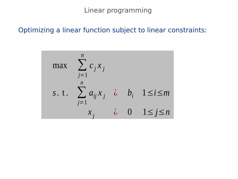
Optimizing a linear function subject to linear constraints:
Linear programming
max ∑j=1
n
c j x j
s . t . ∑j=1
n
aij x j ¿ bi 1≤i≤m
x j ¿ 0 1≤ j≤n
History of linear programming and its applications
Introduction to Linear programming A toy example Geometric intuition Simplex method
A more formal approach to Simplex Basic feasible solutions Implementing Simplex
Computational challenges Are there polynomial time algorithms for LP?
Linear programming duality
Outline of the lecture
7
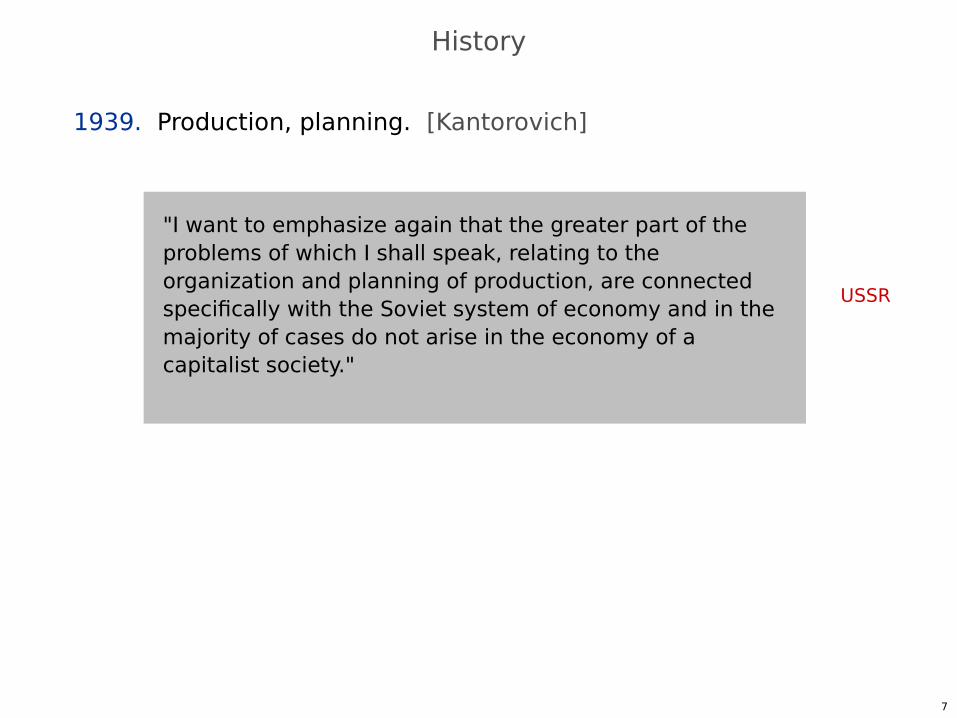
History
1939. Production, planning. [Kantorovich]
USSR
"I want to emphasize again that the greater part of the problems of which I shall speak, relating to the organization and planning of production, are connected specifically with the Soviet system of economy and in the majority of cases do not arise in the economy of a capitalist society."
8
History
1939. Production, planning. [Kantorovich] Kantorovich awarded 1975 Nobel prize in Economics for
contributions to the theory of optimum allocation of resources.
9
History
1939. Production, planning. [Kantorovich]1947. Simplex algorithm. [Dantzig]
10
Berlin Airlift
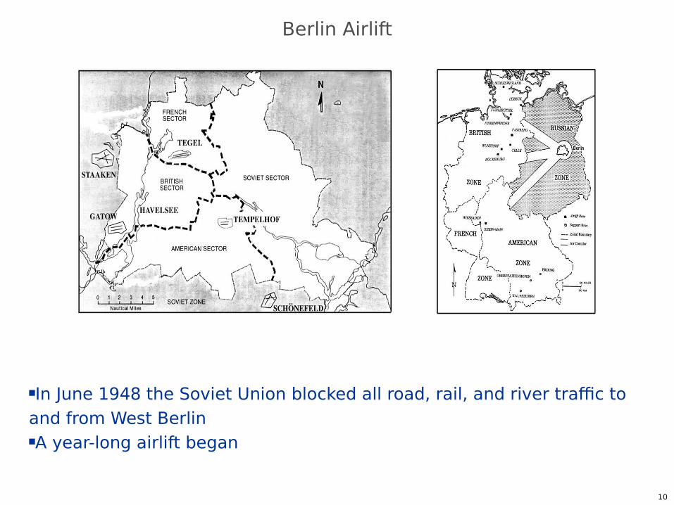
In June 1948 the Soviet Union blocked all road, rail, and river traffic to and from West BerlinA year-long airlift began
11
Berlin Airlift
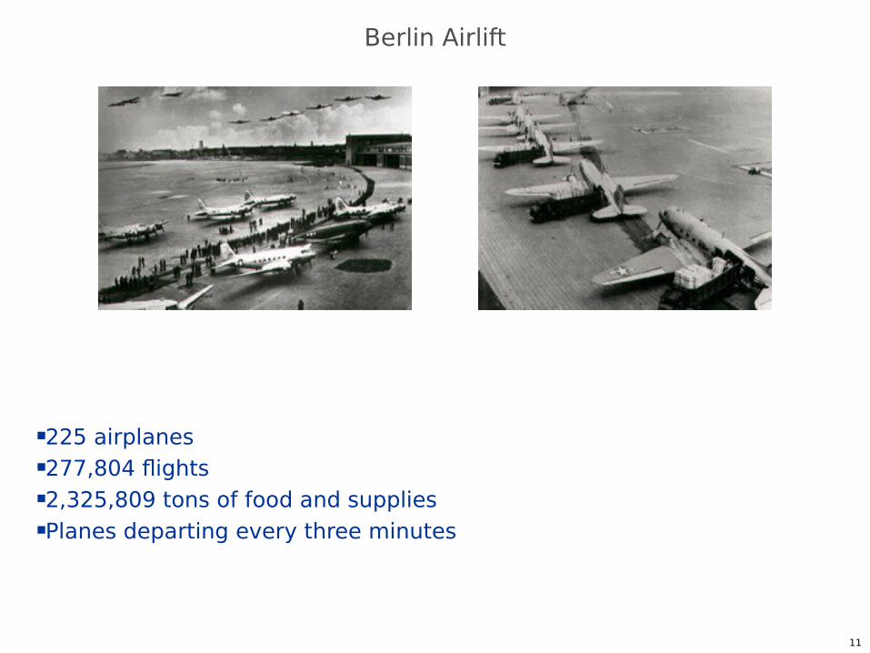
225 airplanes277,804 flights2,325,809 tons of food and suppliesPlanes departing every three minutes
12
Berlin Airlift
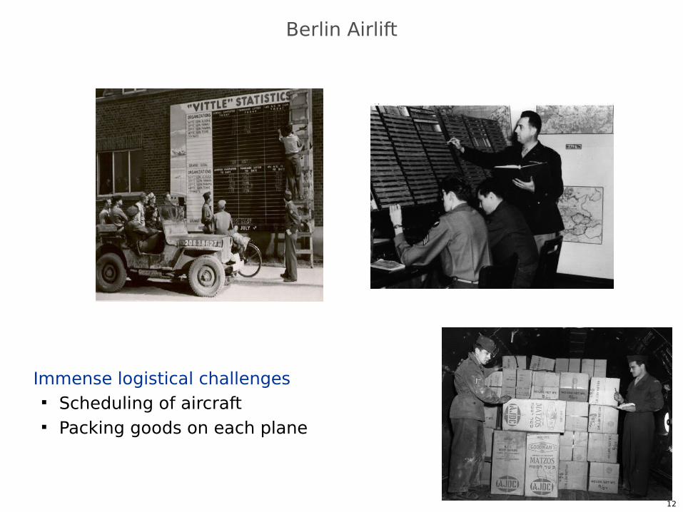
Immense logistical challenges Scheduling of aircraft Packing goods on each plane
13
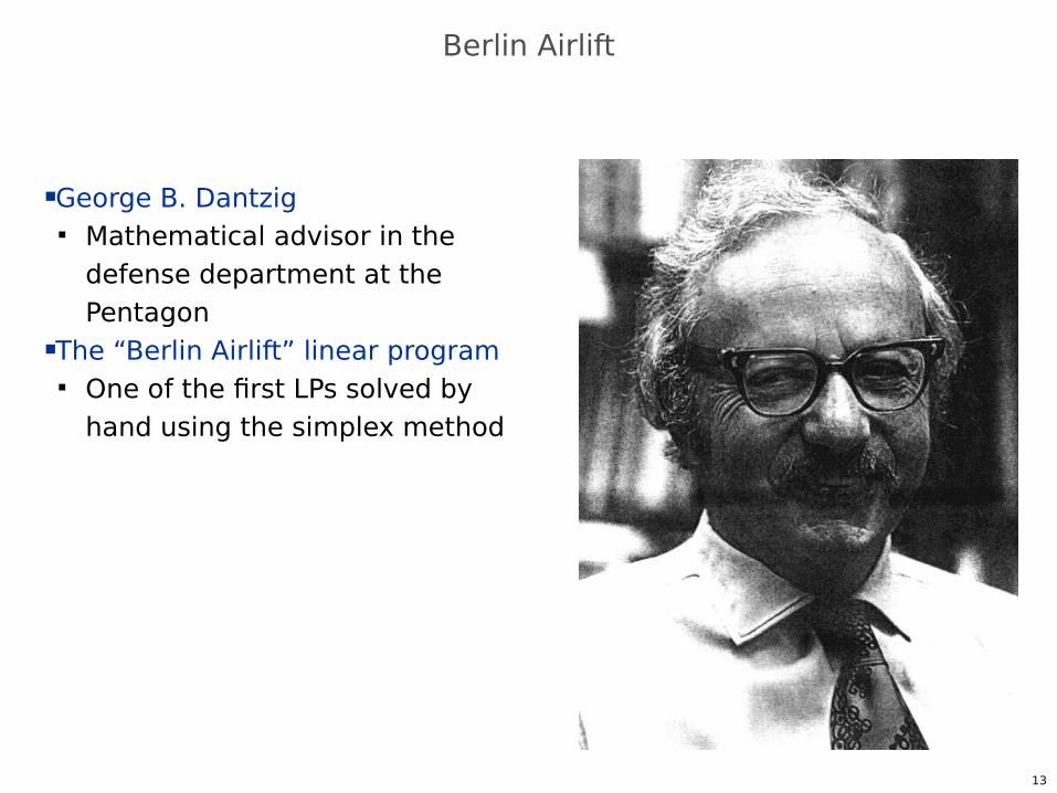
Berlin Airlift
George B. Dantzig Mathematical advisor in the
defense department at the Pentagon
The “Berlin Airlift” linear program One of the first LPs solved by
hand using the simplex method
14
Linear Programming
One of the most influential computational problems of the 20th century
Allocation of limited resources among competing activities so as to optimize an objective
Nobel prize in economics, 1975
15
Linear Programming
Evolved to become… Quintessential tool for optimal allocation of scarce resources,
among a number of competing activities. Powerful and general problem-solving method
Why significant? Fast commercial solvers: CPLEX, OSL. Powerful modeling languages: AMPL, GAMS. Ranked among most important scientific advances of 20th
century. Widely applicable and dominates world of industry.
Ex: Delta claims saving $100 million per year using LP
16
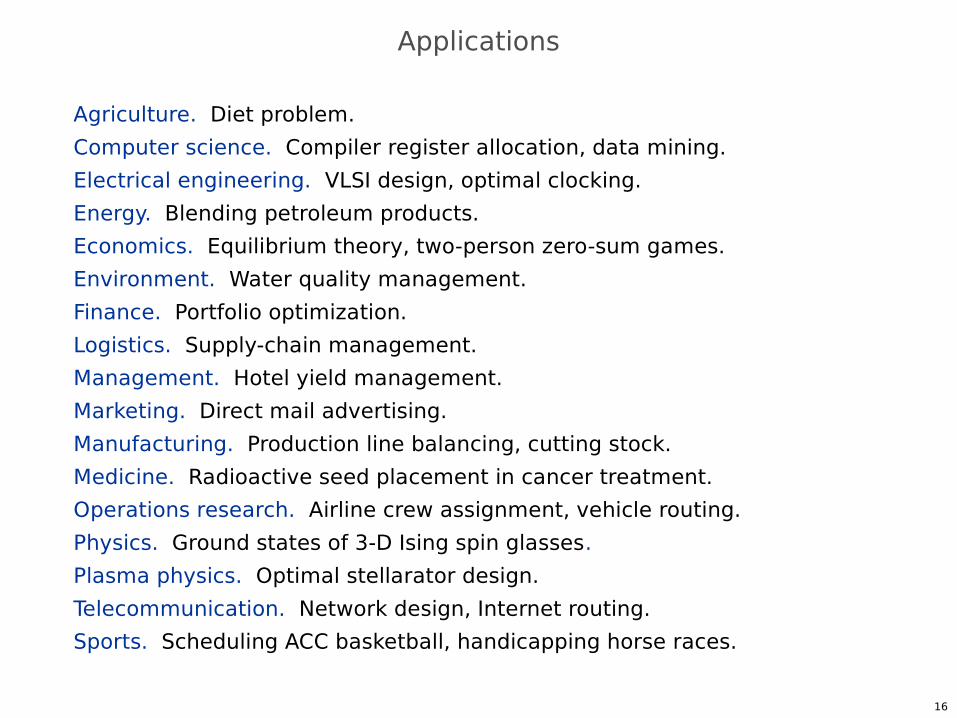
Applications
Agriculture. Diet problem.
Computer science. Compiler register allocation, data mining.
Electrical engineering. VLSI design, optimal clocking.
Energy. Blending petroleum products.
Economics. Equilibrium theory, two-person zero-sum games.
Environment. Water quality management.
Finance. Portfolio optimization.
Logistics. Supply-chain management.
Management. Hotel yield management.
Marketing. Direct mail advertising.
Manufacturing. Production line balancing, cutting stock.
Medicine. Radioactive seed placement in cancer treatment.
Operations research. Airline crew assignment, vehicle routing.
Physics. Ground states of 3-D Ising spin glasses.
Plasma physics. Optimal stellarator design.
Telecommunication. Network design, Internet routing.
Sports. Scheduling ACC basketball, handicapping horse races.
History of linear programming and its applications
Introduction to Linear programming A toy example Geometric intuition Simplex method
A more formal approach to Simplex Basic feasible solutions Implementing Simplex
Computational challenges Are there polynomial time algorithms for LP?
Linear programming duality
Outline of the lecture
18
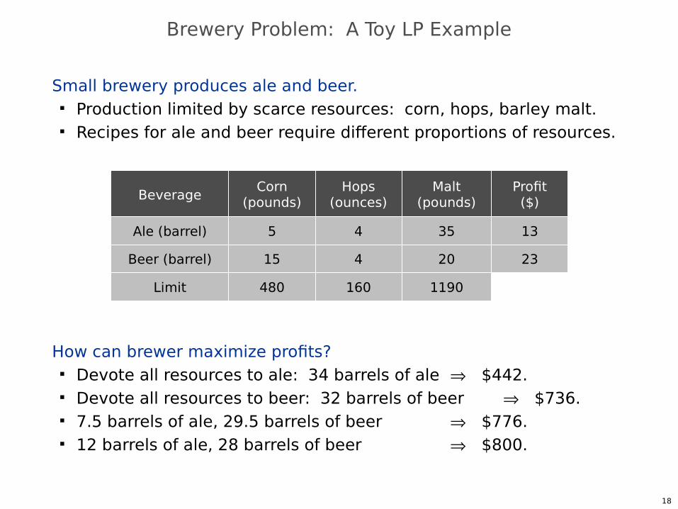
Brewery Problem: A Toy LP Example
Small brewery produces ale and beer. Production limited by scarce resources: corn, hops, barley malt. Recipes for ale and beer require different proportions of resources.
How can brewer maximize profits? Devote all resources to ale: 34 barrels of ale $442. Devote all resources to beer: 32 barrels of beer $736. 7.5 barrels of ale, 29.5 barrels of beer $776. 12 barrels of ale, 28 barrels of beer $800.
BeverageCorn
(pounds)Malt
(pounds)Hops
(ounces)
Beer (barrel) 15 204
Ale (barrel) 5 354
Profit($)
23
13
Limit 480 1190160
19
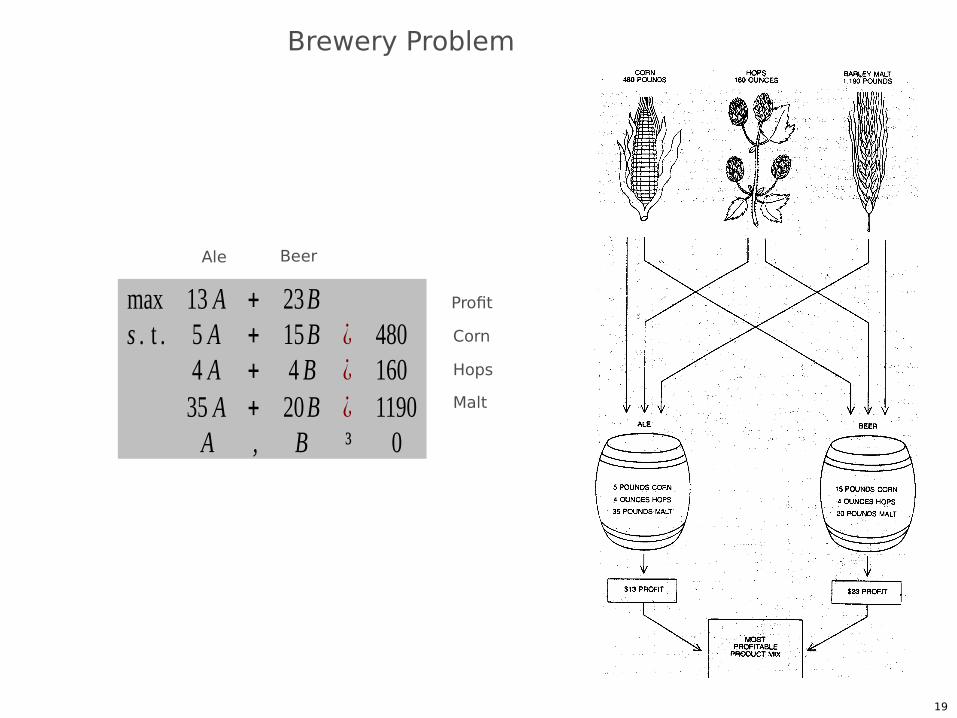
Brewery Problem
max 13 A + 23Bs . t . 5 A + 15B ¿ 480
4 A + 4 B ¿ 16035 A + 20B ¿ 1190A , B ³ 0
Ale Beer
Corn
Hops
Malt
Profit
20
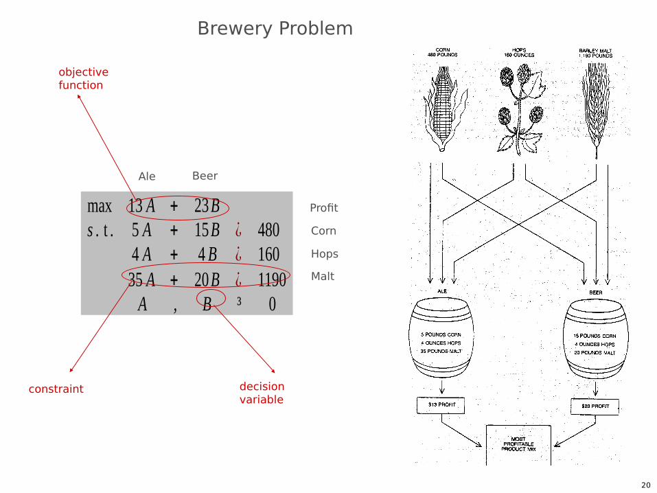
Brewery Problem
max 13 A + 23Bs . t . 5 A + 15B ¿ 480
4 A + 4 B ¿ 16035 A + 20B ¿ 1190A , B ³ 0
Ale Beer
Corn
Hops
Malt
Profit
objective function
constraint decision variable
21
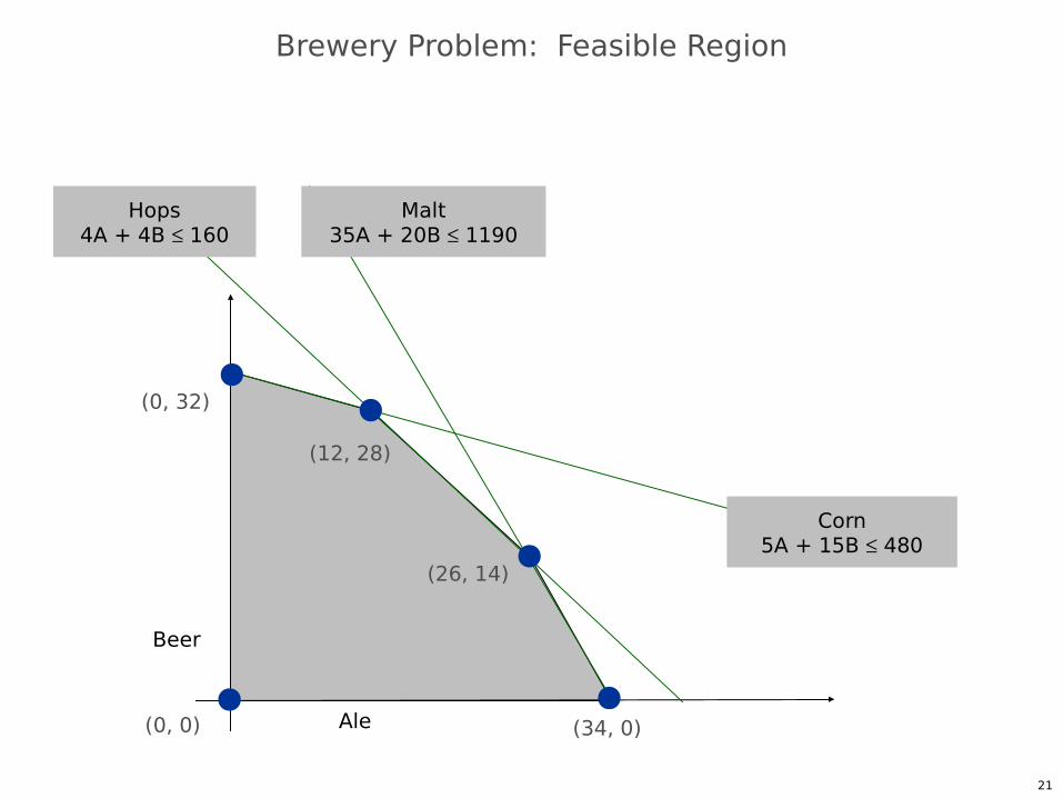
Brewery Problem: Feasible Region
Ale
Beer
(34, 0)
(0, 32)
Corn5A + 15B 480
Hops4A + 4B 160
Malt35A + 20B 1190
(12, 28)
(26, 14)
(0, 0)
22
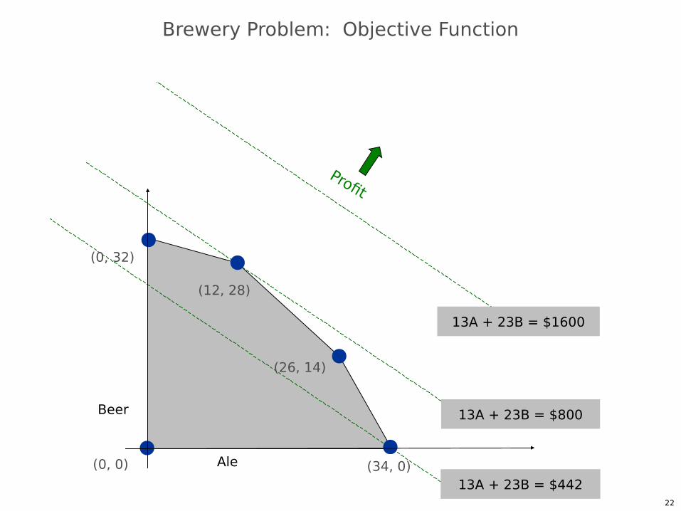
Brewery Problem: Objective Function
13A + 23B = $800
13A + 23B = $1600
13A + 23B = $442(34, 0)
(0, 32)
(12, 28)
(26, 14)
(0, 0)
Profit
Ale
Beer
23
(34, 0)
(0, 32)
(12, 28)
(0, 0)
(26, 14)
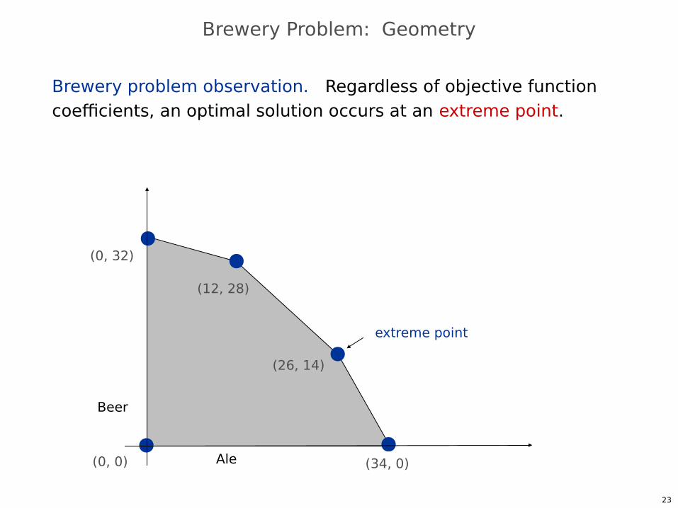
Brewery Problem: Geometry
Brewery problem observation. Regardless of objective function coefficients, an optimal solution occurs at an extreme point.
extreme point
Ale
Beer
24
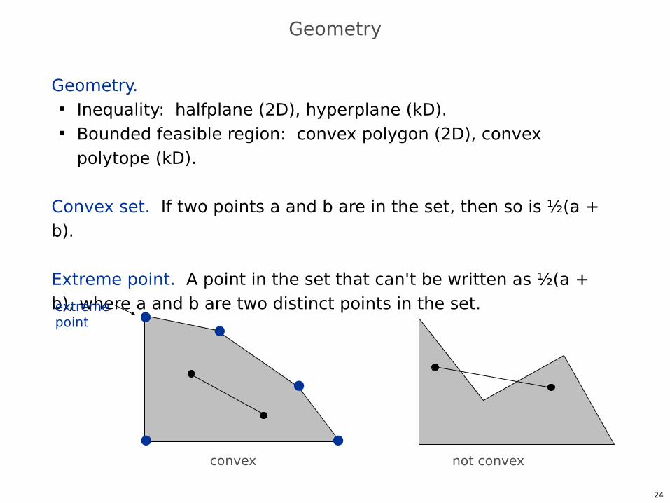
Geometry. Inequality: halfplane (2D), hyperplane (kD). Bounded feasible region: convex polygon (2D), convex
polytope (kD).
Convex set. If two points a and b are in the set, then so is ½(a + b).
Extreme point. A point in the set that can't be written as ½(a + b), where a and b are two distinct points in the set.
Geometry
convex not convex
extremepoint
25
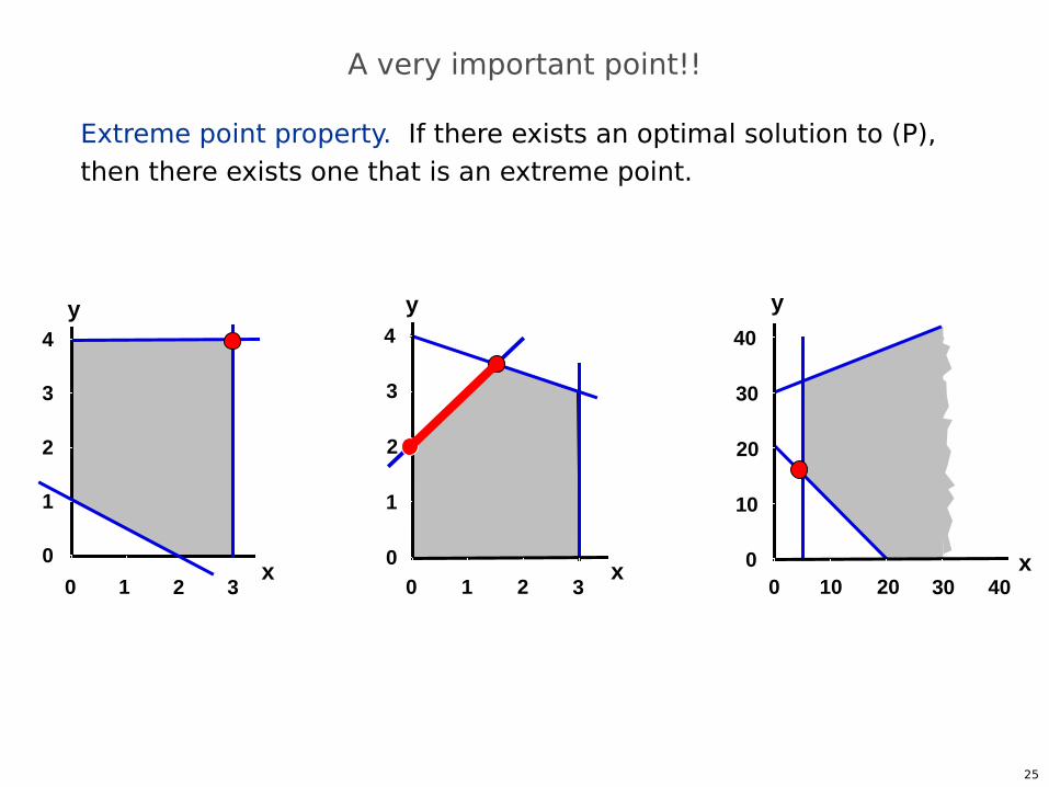
A very important point!!
Extreme point property. If there exists an optimal solution to (P),then there exists one that is an extreme point.
y
x0
1
2
3
4
0 1 2
3
x3010 20
y
0
10
20
40
0
30
40x
y
0
1
2
3
4
0 1 2
3
26
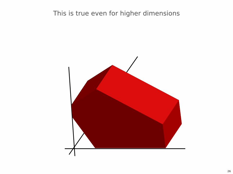
This is true even for higher dimensions
27
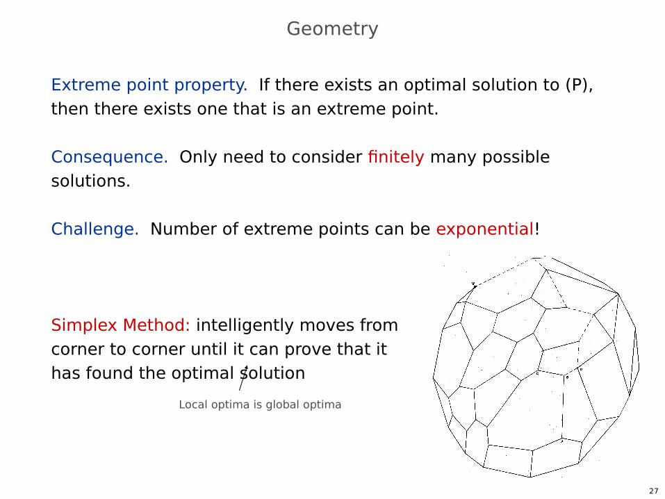
Geometry
Extreme point property. If there exists an optimal solution to (P),then there exists one that is an extreme point.
Consequence. Only need to consider finitely many possible solutions.
Challenge. Number of extreme points can be exponential!
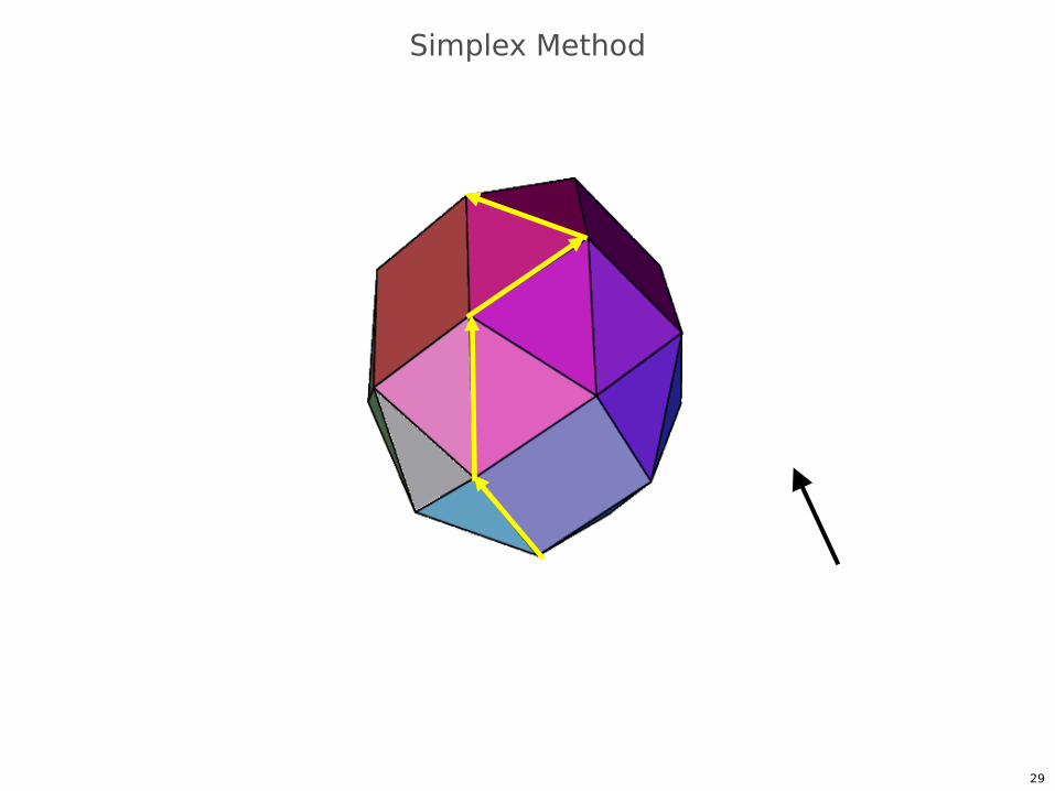
Simplex Method: intelligently moves from corner to corner until it can prove that it has found the optimal solution
Local optima is global optima

28
Linear Programming
29
Simplex Method
History of linear programming and its applications
Introduction to Linear programming A toy example Geometric intuition Simplex method
A more formal approach to Simplex Basic feasible solutions Implementing Simplex
Computational challenges Are there polynomial time algorithms for LP?
Linear programming duality
Outline of the lecture
31
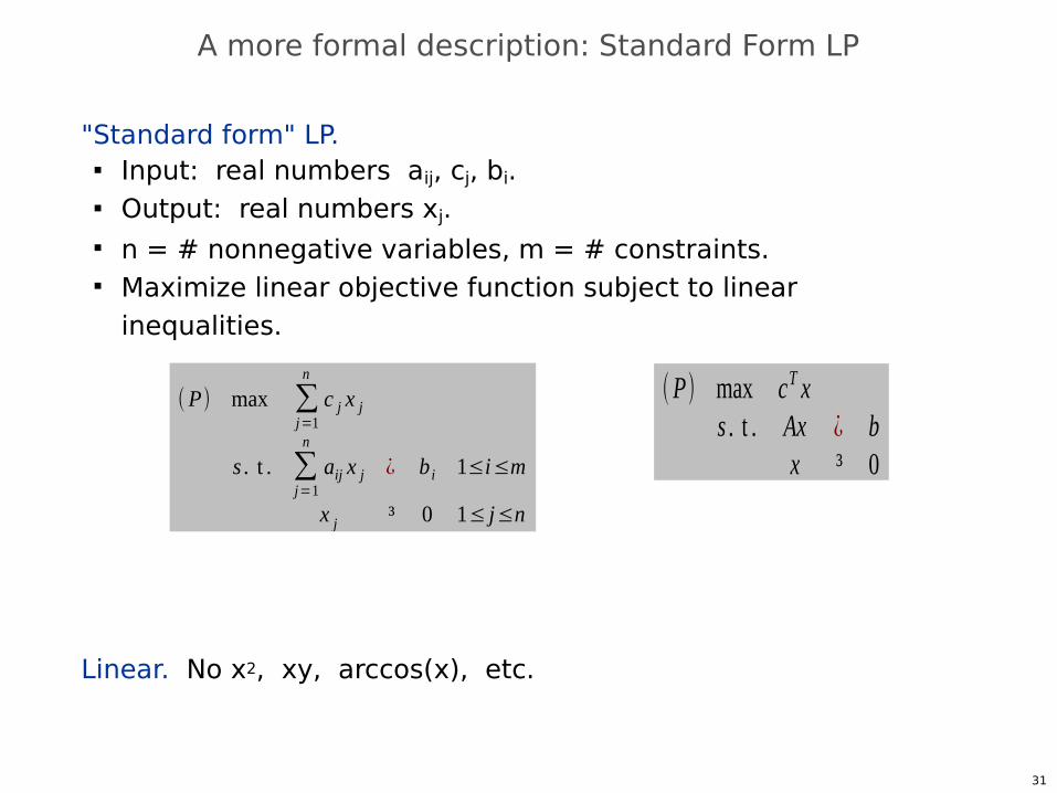
A more formal description: Standard Form LP
"Standard form" LP. Input: real numbers aij, cj, bi. Output: real numbers xj. n = # nonnegative variables, m = # constraints. Maximize linear objective function subject to linear
inequalities.
Linear. No x2, xy, arccos(x), etc.
(P) max ∑j=1
n
c j x j
s . t . ∑j=1
n
aij x j ¿ b i 1≤i≤m
x j ³ 0 1≤ j≤n
(P) max cT xs . t . Ax ¿ b
x ³ 0
32
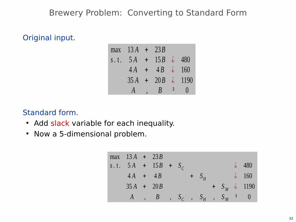
Brewery Problem: Converting to Standard Form
Original input.
Standard form. Add slack variable for each inequality. Now a 5-dimensional problem.
max 13 A + 23Bs . t . 5 A + 15B ¿ 480
4 A + 4 B ¿ 16035 A + 20B ¿ 1190A , B ³ 0
max 13 A + 23Bs . t . 5 A + 15B + SC ¿ 480
4 A + 4 B + SH ¿ 160
35 A + 20B + SM ¿ 1190
A , B , SC , SH , SM ³ 0
33
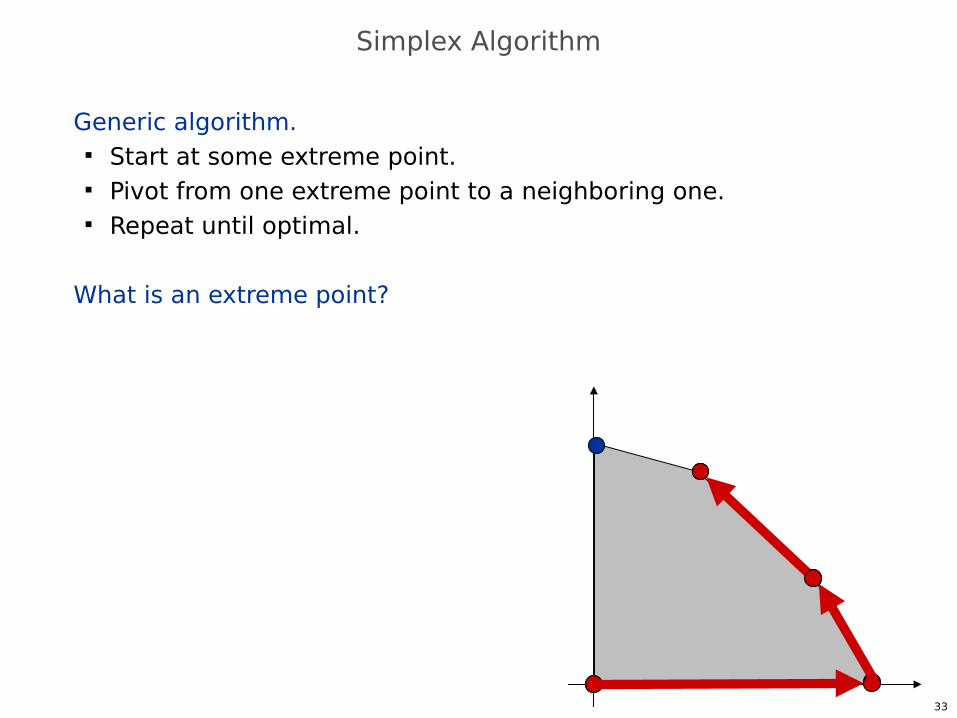
Simplex Algorithm
Generic algorithm. Start at some extreme point. Pivot from one extreme point to a neighboring one. Repeat until optimal.
What is an extreme point?
34
Simplex Algorithm: Basis
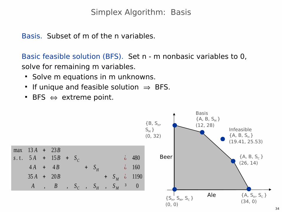
Basis. Subset of m of the n variables.
Basic feasible solution (BFS). Set n - m nonbasic variables to 0,solve for remaining m variables.
Solve m equations in m unknowns. If unique and feasible solution BFS. BFS extreme point.
Ale
Beer
Basis{A, B, SM }(12, 28)
{A, B, SC }(26, 14)
{B, SH, SM }(0, 32)
{SH, SM, SC }(0, 0)
{A, SH, SC }(34, 0)
max 13 A + 23Bs . t . 5 A + 15B + SC ¿ 480
4 A + 4 B + SH ¿ 160
35 A + 20B + SM ¿ 1190
A , B , SC , SH , SM ³ 0
Infeasible{A, B, SH }(19.41, 25.53)
35
Simplex Algorithm: Degeneracy
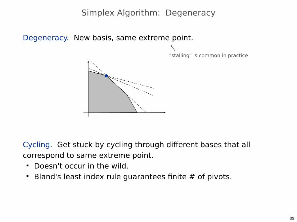
Degeneracy. New basis, same extreme point.
Cycling. Get stuck by cycling through different bases that all correspond to same extreme point.
Doesn't occur in the wild. Bland's least index rule guarantees finite # of pivots.
"stalling" is common in practice
36
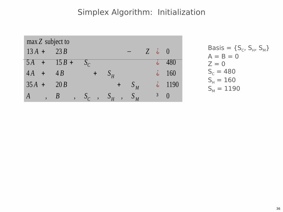
Simplex Algorithm: Initialization
Basis = {SC, SH, SM}A = B = 0Z = 0SC = 480 SH = 160 SM = 1190
max Z subject to13 A + 23 B − Z ¿ 05 A + 15 B + SC ¿ 4804 A + 4 B + SH ¿ 160
35 A + 20 B + SM ¿ 1190
A , B , SC , SH , SM ³ 0
37
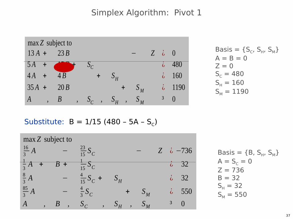
max Z subject to163
A − 2315
SC − Z ¿ −7361
3A + B +
1
15SC ¿ 32
83
A −415
SC + SH ¿ 32853
A −43SC + SM ¿ 550
A , B , SC , SH , SM ³ 0
Basis = {B, SH, SM}A = SC = 0Z = 736B = 32SH = 32SM = 550
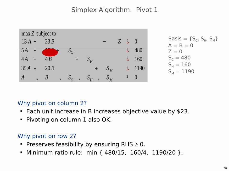
Simplex Algorithm: Pivot 1
Substitute: B = 1/15 (480 – 5A – SC)
Basis = {SC, SH, SM}A = B = 0Z = 0SC = 480 SH = 160 SM = 1190
max Z subject to13 A + 23 B − Z ¿ 05 A + 15 B + SC ¿ 4804 A + 4 B + SH ¿ 160
35 A + 20 B + SM ¿ 1190
A , B , SC , SH , SM ³ 0
38
Simplex Algorithm: Pivot 1
Why pivot on column 2? Each unit increase in B increases objective value by $23. Pivoting on column 1 also OK.
Why pivot on row 2? Preserves feasibility by ensuring RHS 0. Minimum ratio rule: min { 480/15, 160/4, 1190/20 }.
max Z subject to13 A + 23 B − Z ¿ 05 A + 15 B + SC ¿ 4804 A + 4 B + SH ¿ 160
35 A + 20 B + SM ¿ 1190
A , B , SC , SH , SM ³ 0
Basis = {SC, SH, SM}A = B = 0Z = 0SC = 480 SH = 160 SM = 1190
39
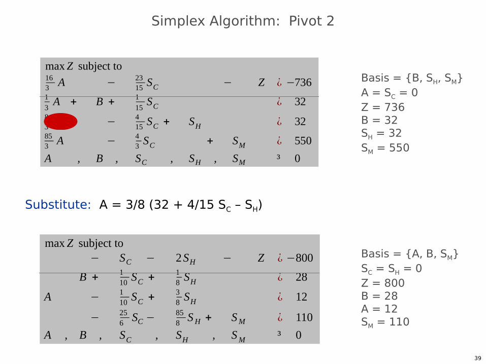
Simplex Algorithm: Pivot 2
max Z subject to163
A −2315
SC − Z ¿ −7361
3A + B +
1
15SC ¿ 32
83
A −415
SC + SH ¿ 32853
A −43SC + SM ¿ 550
A , B , SC , SH , SM ³ 0
max Z subject to− SC − 2SH − Z ¿ −800
B +110
SC +18SH ¿ 28
A −110
SC +38SH ¿ 12
−256
SC −858
SH + SM ¿ 110
A , B , SC , SH , SM ³ 0
Substitute: A = 3/8 (32 + 4/15 SC – SH)
Basis = {B, SH, SM}A = SC = 0Z = 736B = 32SH = 32SM = 550
Basis = {A, B, SM}SC = SH = 0Z = 800B = 28A = 12SM = 110
40
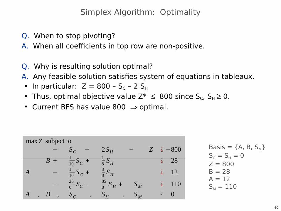
Simplex Algorithm: Optimality
Q. When to stop pivoting?A. When all coefficients in top row are non-positive.
Q. Why is resulting solution optimal?A. Any feasible solution satisfies system of equations in tableaux.
In particular: Z = 800 – SC – 2 SH
Thus, optimal objective value Z* 800 since SC, SH 0. Current BFS has value 800 optimal.
Basis = {A, B, SM}SC = SH = 0Z = 800B = 28A = 12SM = 110
max Z subject to− SC − 2SH − Z ¿ −800
B +110
SC +18SH ¿ 28
A −110
SC +38SH ¿ 12
−256
SC −858
SH + SM ¿ 110
A , B , SC , SH , SM ³ 0
41
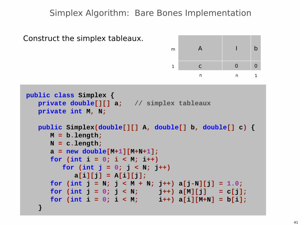
Simplex Algorithm: Bare Bones Implementation
Construct the simplex tableaux.A
c
bI
0 0
public class Simplex { private double[][] a; // simplex tableaux private int M, N;
public Simplex(double[][] A, double[] b, double[] c) { M = b.length; N = c.length; a = new double[M+1][M+N+1]; for (int i = 0; i < M; i++) for (int j = 0; j < N; j++) a[i][j] = A[i][j]; for (int j = N; j < M + N; j++) a[j-N][j] = 1.0; for (int j = 0; j < N; j++) a[M][j] = c[j]; for (int i = 0; i < M; i++) a[i][M+N] = b[i]; }
m
1
n n 1
42
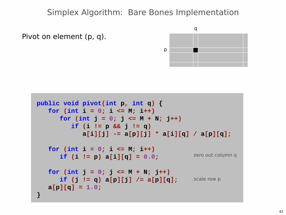
Simplex Algorithm: Bare Bones Implementation
Pivot on element (p, q).
public void pivot(int p, int q) { for (int i = 0; i <= M; i++) for (int j = 0; j <= M + N; j++) if (i != p && j != q) a[i][j] -= a[p][j] * a[i][q] / a[p][q]; for (int i = 0; i <= M; i++) if (i != p) a[i][q] = 0.0;
for (int j = 0; j <= M + N; j++) if (j != q) a[p][j] /= a[p][q]; a[p][q] = 1.0;}
zero out column q
scale row p
p
q
43
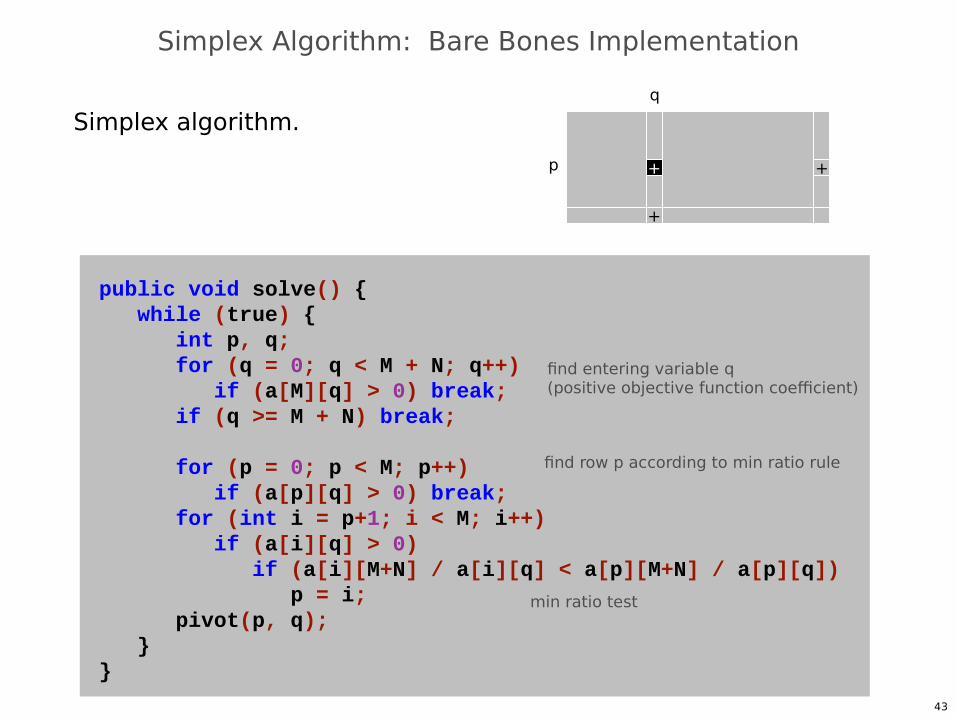
Simplex Algorithm: Bare Bones Implementation
Simplex algorithm.
public void solve() { while (true) { int p, q; for (q = 0; q < M + N; q++) if (a[M][q] > 0) break; if (q >= M + N) break;
for (p = 0; p < M; p++) if (a[p][q] > 0) break; for (int i = p+1; i < M; i++) if (a[i][q] > 0) if (a[i][M+N] / a[i][q] < a[p][M+N] / a[p][q]) p = i; pivot(p, q); }}
find entering variable q(positive objective function coefficient)
find row p according to min ratio rule
min ratio test
+p
q
+
+
History of linear programming and its applications
Introduction to Linear programming A toy example Geometric intuition Simplex method
A more formal approach to Simplex Basic feasible solutions Implementing Simplex
Computational challenges Are there polynomial time algorithms for LP?
Linear programming duality
Outline of the lecture
45
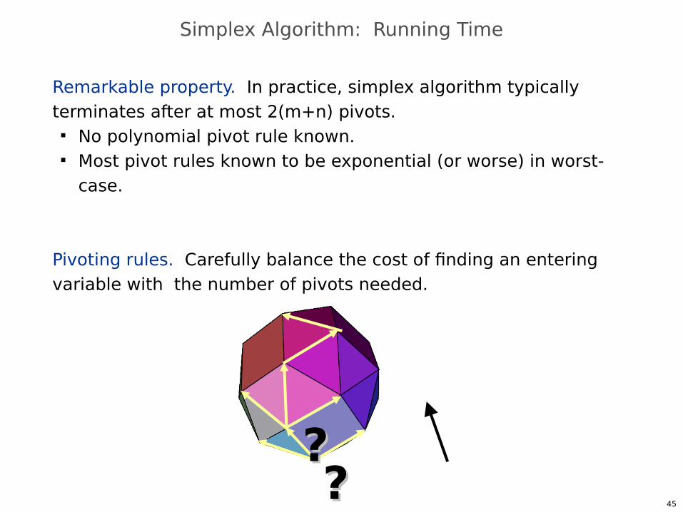
Simplex Algorithm: Running Time
Remarkable property. In practice, simplex algorithm typically terminates after at most 2(m+n) pivots.
No polynomial pivot rule known. Most pivot rules known to be exponential (or worse) in worst-
case.
Pivoting rules. Carefully balance the cost of finding an entering variable with the number of pivots needed.
????
Simplex Algorithm
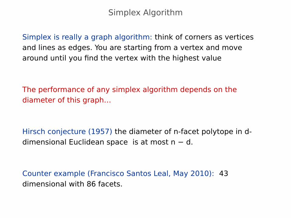
Simplex is really a graph algorithm: think of corners as vertices and lines as edges. You are starting from a vertex and move around until you find the vertex with the highest value
The performance of any simplex algorithm depends on the diameter of this graph…
Hirsch conjecture (1957) the diameter of n-facet polytope in d-dimensional Euclidean space is at most n − d.
Counter example (Francisco Santos Leal, May 2010): 43 dimensional with 86 facets.
47
Simplex Algorithm: Implementation Issues
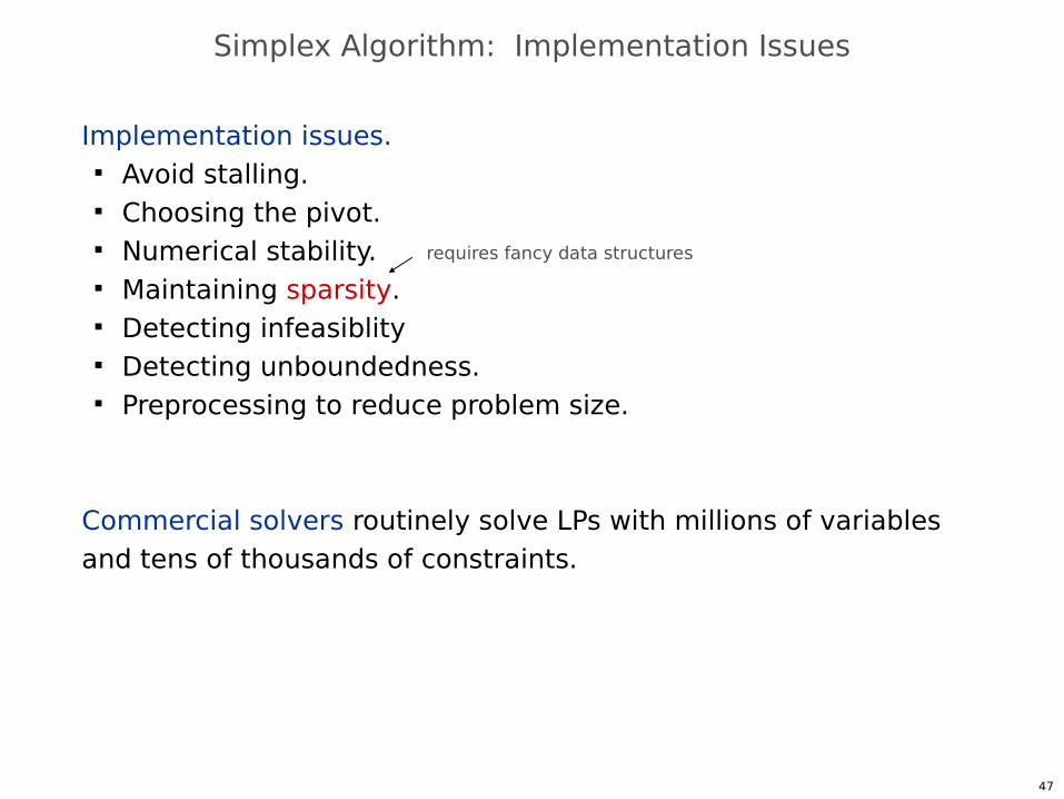
Implementation issues. Avoid stalling. Choosing the pivot. Numerical stability. Maintaining sparsity. Detecting infeasiblity Detecting unboundedness. Preprocessing to reduce problem size.
Commercial solvers routinely solve LPs with millions of variables and tens of thousands of constraints.
requires fancy data structures
48
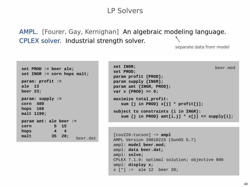
set PROD := beer ale;set INGR := corn hops malt;
param: profit :=ale 13beer 23;
param: supply :=corn 480hops 160malt 1190;
param amt: ale beer :=corn 5 15hops 4 4malt 35 20;
LP Solvers
AMPL. [Fourer, Gay, Kernighan] An algebraic modeling language.CPLEX solver. Industrial strength solver.
set INGR;set PROD;param profit {PROD};param supply {INGR};param amt {INGR, PROD};var x {PROD} >= 0;
maximize total_profit: sum {j in PROD} x[j] * profit[j];
subject to constraints {i in INGR}: sum {j in PROD} amt[i,j] * x[j] <= supply[i];
beer.dat
beer.mod
[cos226:tucson] ~> amplAMPL Version 20010215 (SunOS 5.7)ampl: model beer.mod;ampl: data beer.dat;ampl: solve;CPLEX 7.1.0: optimal solution; objective 800ampl: display x;x [*] := ale 12 beer 28;
separate data from model
49
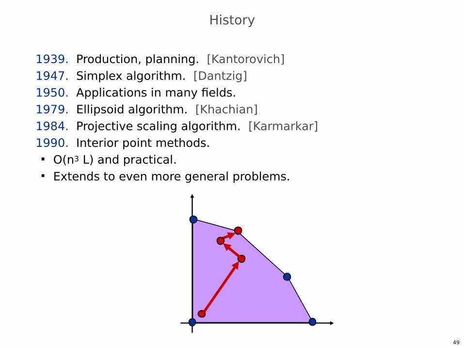
History
1939. Production, planning. [Kantorovich]1947. Simplex algorithm. [Dantzig]1950. Applications in many fields.1979. Ellipsoid algorithm. [Khachian]1984. Projective scaling algorithm. [Karmarkar]1990. Interior point methods.
O(n3 L) and practical. Extends to even more general problems.
50
History
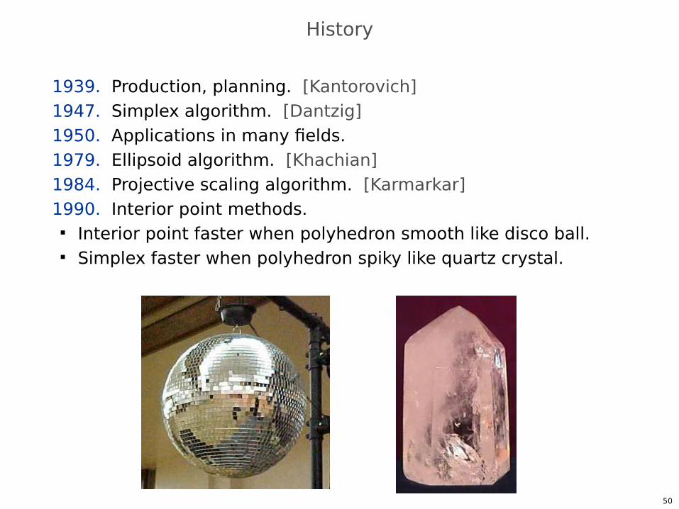
1939. Production, planning. [Kantorovich]1947. Simplex algorithm. [Dantzig]1950. Applications in many fields.1979. Ellipsoid algorithm. [Khachian]1984. Projective scaling algorithm. [Karmarkar]1990. Interior point methods.
Interior point faster when polyhedron smooth like disco ball. Simplex faster when polyhedron spiky like quartz crystal.
51
Rest of the history…
1939. Production, planning. [Kantorovich]1947. Simplex algorithm. [Dantzig]1950. Applications in many fields.1979. Ellipsoid algorithm. [Khachian]1984. Projective scaling algorithm. [Karmarkar]
O(n3.5 L). Efficient implementations possible.
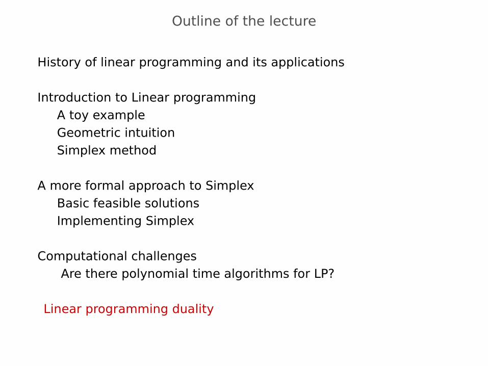
History of linear programming and its applications
Introduction to Linear programming A toy example Geometric intuition Simplex method
A more formal approach to Simplex Basic feasible solutions Implementing Simplex
Computational challenges Are there polynomial time algorithms for LP?
Linear programming duality
Outline of the lecture
53
LP Duality (Economic Interpretation)
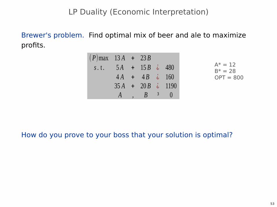
Brewer's problem. Find optimal mix of beer and ale to maximize profits.
How do you prove to your boss that your solution is optimal?
(P)max 13 A + 23 Bs . t . 5 A + 15 B ¿ 480
4 A + 4 B ¿ 16035 A + 20 B ¿ 1190A , B ³ 0
A* = 12B* = 28 OPT = 800
54
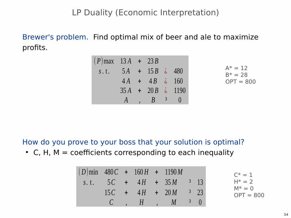
LP Duality (Economic Interpretation)
Brewer's problem. Find optimal mix of beer and ale to maximize profits.
How do you prove to your boss that your solution is optimal? C, H, M = coefficients corresponding to each inequality
(P)max 13 A + 23 Bs . t . 5 A + 15 B ¿ 480
4 A + 4 B ¿ 16035 A + 20 B ¿ 1190A , B ³ 0
(D)min 480C + 160 H + 1190 Ms . t . 5C + 4 H + 35 M ³ 13
15C + 4 H + 20 M ³ 23C , H , M ³ 0
A* = 12B* = 28 OPT = 800
C* = 1H* = 2 M* = 0OPT = 800
55
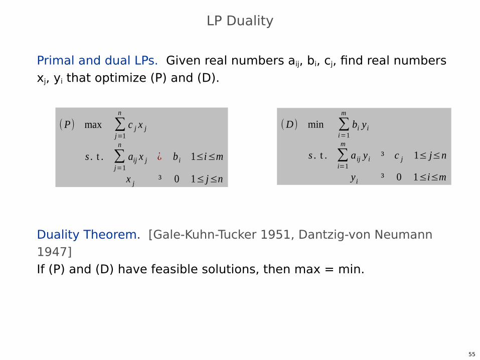
Primal and dual LPs. Given real numbers aij, bi, cj, find real numbers xj, yi that optimize (P) and (D).
Duality Theorem. [Gale-Kuhn-Tucker 1951, Dantzig-von Neumann 1947]If (P) and (D) have feasible solutions, then max = min.
(P) max ∑j=1
n
c j x j
s . t . ∑j=1
n
aij x j ¿ b i 1≤i≤m
x j ³ 0 1≤ j≤n
(D) min ∑i=1
m
bi yi
s . t . ∑i=1
m
a ij y i ³ c j 1≤ j≤n
y i ³ 0 1≤i≤m
LP Duality
56
LP Duality: Sensitivity Analysis
Q. How much should brewer be willing to pay (marginal price) for additional supplies of scarce resources?A. Corn $1, hops $2, malt $0.
57
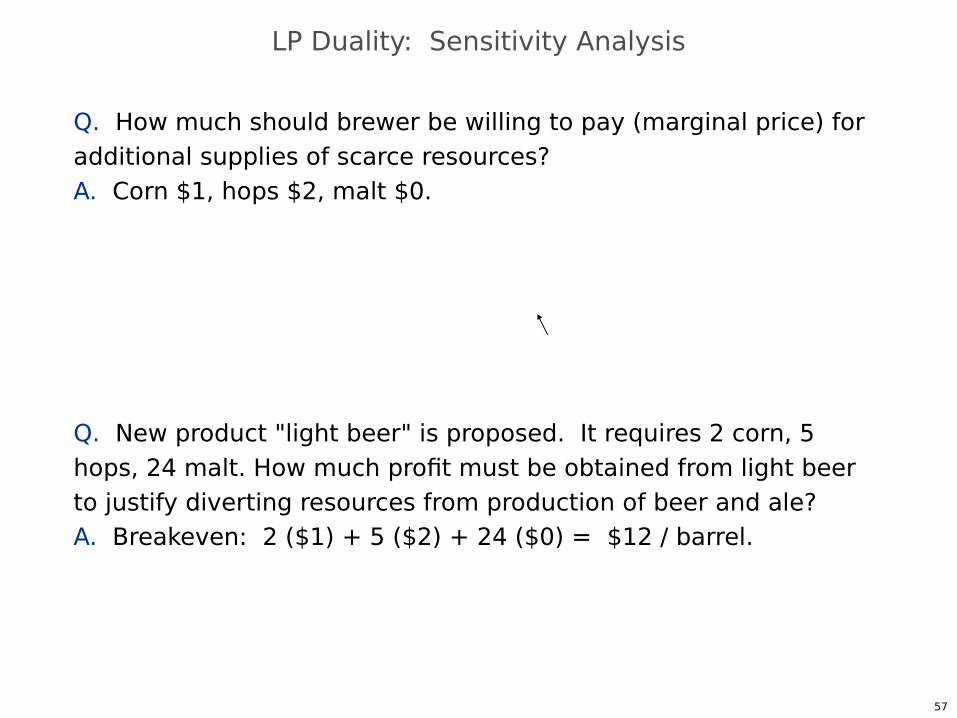
LP Duality: Sensitivity Analysis
Q. How much should brewer be willing to pay (marginal price) for additional supplies of scarce resources?A. Corn $1, hops $2, malt $0.
Q. New product "light beer" is proposed. It requires 2 corn, 5 hops, 24 malt. How much profit must be obtained from light beer to justify diverting resources from production of beer and ale?A. Breakeven: 2 ($1) + 5 ($2) + 24 ($0) = $12 / barrel.
58
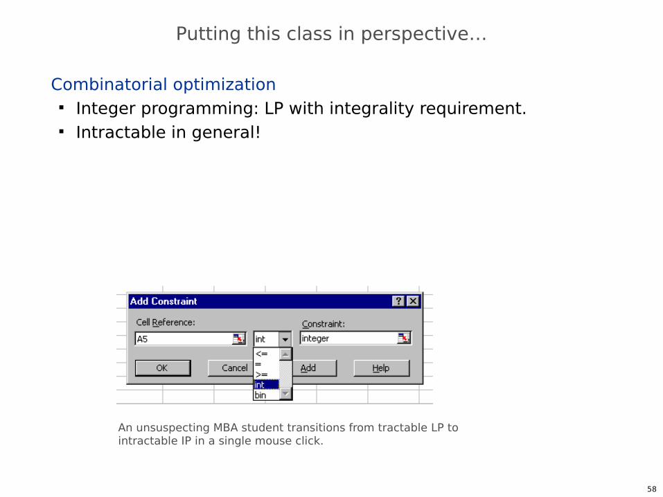
Putting this class in perspective…
Combinatorial optimization Integer programming: LP with integrality requirement. Intractable in general!
An unsuspecting MBA student transitions from tractable LP to intractable IP in a single mouse click.
59
x
y
0
1
2
3
4
0 1 2
3
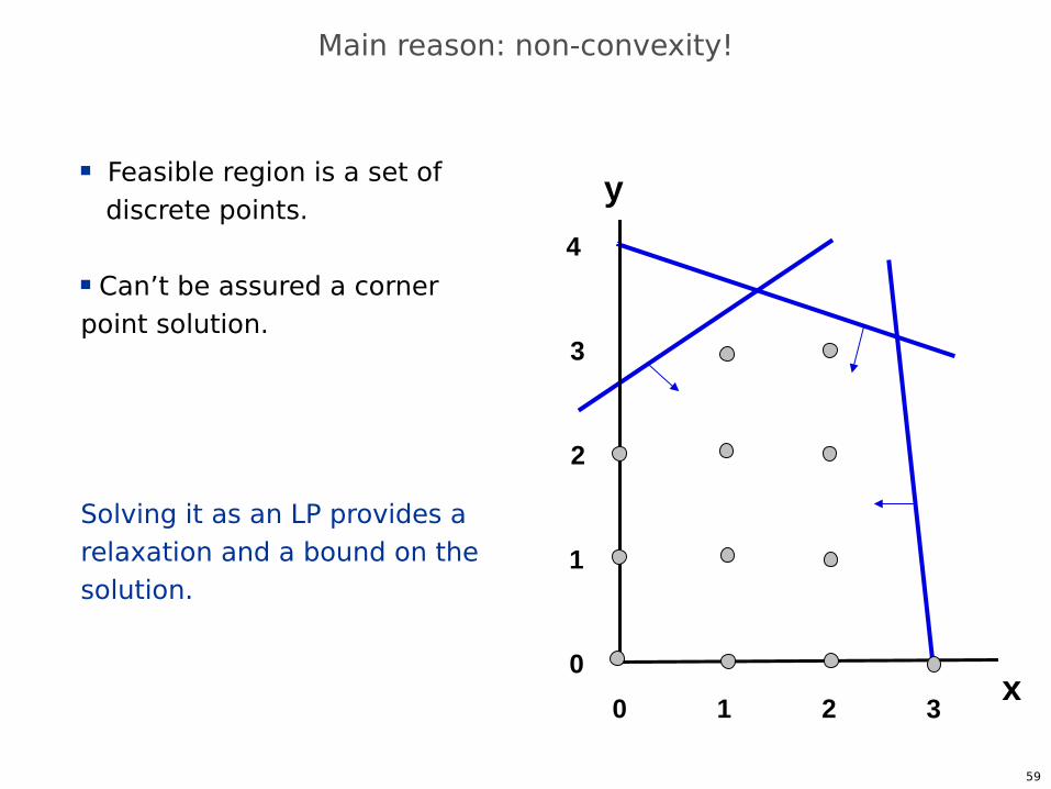
Main reason: non-convexity!
Feasible region is a set of discrete points.
Can’t be assured a corner point solution.
Solving it as an LP provides a relaxation and a bound on the solution.
60
x
y
0
1
2
3
4
0 1 2
3
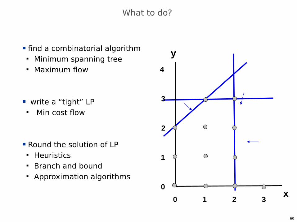
What to do?
find a combinatorial algorithm Minimum spanning tree Maximum flow
write a “tight” LP Min cost flow
Round the solution of LP Heuristics Branch and bound Approximation algorithms