linear programming using the simplex …/67531/metadc130787/...linear programming using the simplex...
TRANSCRIPT
LINEAR PROGRAMMING USING THE SIMPLEX METHOD
APPROVED:
-7 / /
Major Prcffessor //
I' ^<fi 4- &~ck Minor Professor
JTT miojuf Director of the Department of Mathematics
O _____
Dean of the Graduate School
LINEAR PROGRAMMING USING THE SIMPLEX METHOD
THESIS
Presented to the Graduate Council of the
North Texas State University in Partial
Fulfillment of the Requirements
For the Degree of
MASTER OF ARTS
By
Niram. F. Patterson, Jr.,
Denton, Texas
January, 1967
' TABLE OF CONTENTS
Chapter Page
I. INTRODUCTION I
II. SIMPLEX METHOD . . Ik
III. COMPUTATIONAL ASPECTS OF THE SIMPLEX METHOD 45
BIBLIOGRAPHY 67
ill
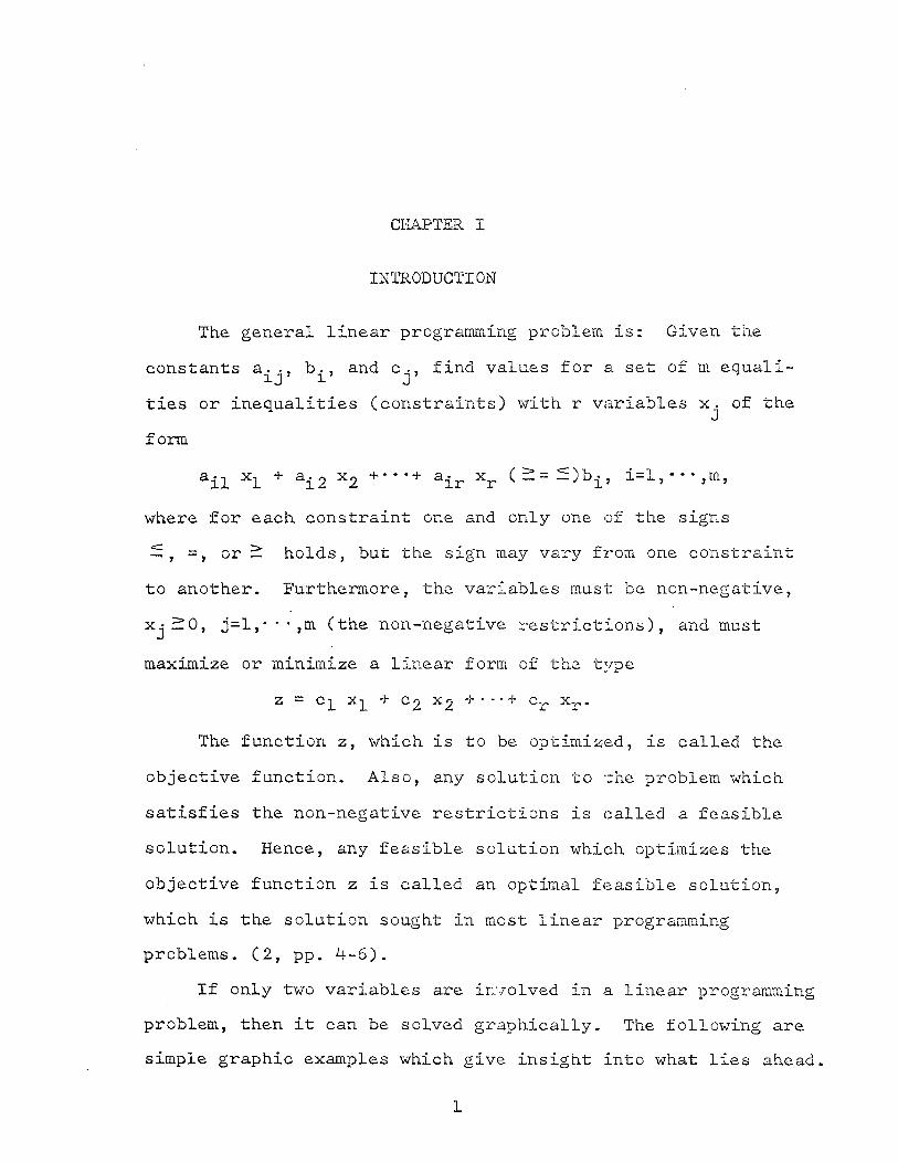
CHAPTER I
INTRODUCTION
The general linear programming problem is: Given the
constants a. b., and c., find values for a set of m equali-1j» i' j'
ties or inequalities (constraints) with r variables x_j of the
form
ail X1 + ai2 x2 +'*"+ air xr ( - = - % , i=l}-**,m,
where for each constraint one and only one of the signs
= , or - holds, but the sign may vary from one constraint
to another. Furthermore, the variables must be non-negative,
XjSO, j=l,- " ' ,m (the non-negative restrictions), and must
maximize or minimize a linear form of the type
z = C]_ X|_ + C£ X2 +*••+ cr xr.
The function z, which is to be optimized, is called the
objective function. Also, any solution to the problem which
satisfies the non-negative restrictions is called a feasible
solution. Hence, any feasible solution which optimizes the
objective function z is called an optimal feasible solution,
which is the solution sought in most linear programming
problems. (2, pp. 4-6).
If only two variables are involved in a linear programming
problem, then it can be solved graphically. The following are
simple graphic examples which give insight into what lies ahead.
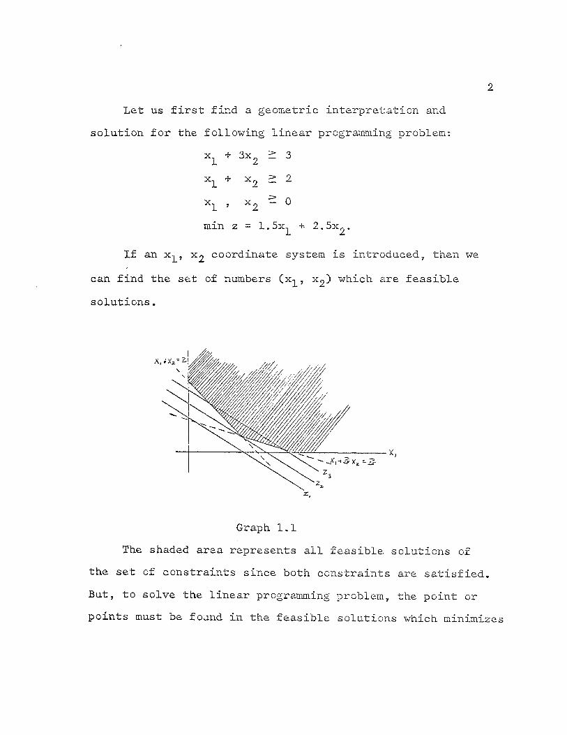
Let us first find a geometric interpretation and,
solution for the following linear programming problem:
x + 3X£ > 3
xx + x 2 2 2
X, X, 0
min z = 1.5x^ +• 2.5x9.
If an x- , X2 coordinate system is introduced, then we
can find the set of numbers (x^, X2) which are feasible
solutions.
Graph 1.1
The shaded area represents all feasible, solutions of
the set of constraints since both constraints are satisfied.
But, to solve the linear programming problem, the point or
points must be found, in the feasible solutions which minimizes
the objective function. If z is a constant, the objective
function becomes a straight line. In Graph 1.1, zL > z 2 > z
3»
but z^ does not have any points on its line that is a feasible
solution. Thus, z £ is the minimum of z, and the feasible
solution which yields this minimum is where the two lines
x + 3x = 3 and x, + x9 = 2 intersect. Solving the equations L 2 L ^
simultaneously, xL = 3/2 and, x 2 = 1/2. Thus, the optimal
feasible solution is min z — 3.5.
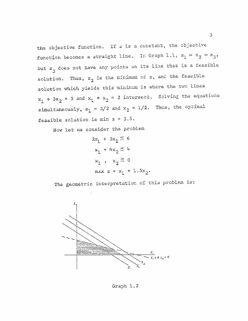
Now let us consider the problem
2Xl + 3X2 -- 6
x^ + S: 4
x x — 0 X 1 ' 2
max z = x^ + 1.5x2*
The geometric interpretation of this problem is:
X,4 4X1*4
Graph 1.2

Clearly, is the maximum value of z. However, the
line which represents the objective function lies along the
edge of the polygon of the feasible solutions. Hence, the
maximum value of z is unique, but there exist an infinite
number of x£) which optimize z. Therefore, there exist
alternative optima, or there exist an infinite number of
optimal feasible solutions.
Next let us consider the problem
X1 " -5x2 - °
5X22-5
1 ' 2
min z = x
0
1 - 1 0 x 2 -
The geometric interpretation of this problem is:
Graph 1.3

If this line is moved parallel to itself in the direction
of increasing z, then it is clear that this could continue
indefinitely. Hence, there exists an unbounded solution since
z can be made arbitrarily large; and therefore, the problem
has no finite maximum value of z. This would not occur in a
practical application, however, since it would imply the
feasibility of an infinite profit.
The final problem wa will consider is
X1 * X2 1
-.5xl - 5X2 -10
X1 J X2 0
max z = -5x
Xif /
Graph 1.4
6
Clearly, this problem has no solution, for the constraints
are inconsistent; for there is no point (x ,, xz) which satis-
fies both constraints.
In order to simplify later discussions on linear programing,
some topics and notation from linear algebra will be needed
(1, pp. 108-123).
Def. 1.1 A matrix is defined to be a rectangular array
of numbers and is written as follows:
A = ij
*11
l21
12 ' l22 *
a. In l2n
el mi ra2 * * ~ ~mn_
and is called a m x n matrix.
Def. 1.2 Two matrices A, 3 are equal if and only if the
corresponding elements are equal, i.e., b^j for every i, j
Def. 1.3 If A is a matrix and A is a real number, then
A a = Aa. ij
Def. 1.4 The identity matrix I of the order n is a
square matrix having ones along the main diagonal and zeros
elsewhere.
where Xjj = f ]
s.. 1J
0 i / j
pL 0 0 • ! o i o • ! o o i •
• o~! - o I - 0
ij " (.1 i = J
|_0 ° ° - - - L
is called the Kronecker delta.

7
Def. 1.5 A matrix whose elements are all zero is called
z:.e. null or zero matrix and is denoted by 0., ]
is a
a1
Def. 1.6 The transpose of a matrix A =
{
matrix A' such that A' = Ila..I !i
Def. 1.7 If all but k rows and s columns are crossed,
out of a m x n matrix A, the resulting k x s matrix is called
a submatrix of A.
Def. 1.8 The determinant of an n-order matrix A = ja-,-
^ j = 2 a l i a2j " " " artv° wn-ere the surn taken over all
permutations of the second subscript. A term is assigned a
plus sign if (i, j, * * •, r) is an even permutation of
(1, 2, • • -, n) and a minus sign if it is an odd permutation.
Def. 1.9 Let A be a matrix. Then A _. is called the co-
factor of element a^- if A ^ is (-l)^4^' tim.es the determinant
of the submatrix obtained, by crossing out row i and. column j
of A.
Def. 1.10 The matrix A + is called the. adjoint of the
matrix A if A* is the transpose of the matrix obtained, from
A by replacing each element a-. by its cofactor at.. j x j
Def. 1.11 Let A be a square matrix. If there exists a
square matrix B which satisfies the relation BA = AB = I,
then B is called the inverse of A.
Def. 1.12 The square matrix A is said to be singular
if A j = 0 ; nonsingular if A / 0.

8
Theorem 1.1 The inverse of a nonsingular matrix A is
unique.
Proof: Suppose there exist two matrices B and G such
that AB = BA = I and AD = DA = I. Since AB = BA = I, then
DAB = DI = D, or IB = D, or B = D.
Hence, the inverse is unique.
Def. 1.13 Matrices having a single row or column are
called vectors and are denoted by a = (a- , - - • , an) or
a = aL, - • a n , where a is a row vector or column
vector, respectively.
Def. 1.14 A unit vector e^ is a vector with unity as
its i - th component and all other components zero.
Def. 1.15 The null vector 0, or zero vector, is a
vector all of whose components are zero.
Def. 1.16 An n-dimensional Euclidean space En is the
collection of all vectors a = [ai» * " " an] - I or these
vectors, addition and scalar multiplication are defined by
the rules for matrix operations.
Def. 1.17 A vector a from En is said to be a linear
combination of the vectors a^, - - •, a^ from En if a can be
written as
^ — ^ ]_ a- •}» /( 2^2 ^ * ri" /I
for some set of scalars.

9
Def. 1.18 A set of vectors aL, • • • f r o m En is said
to be linearly dependent if there exists A not all zero such
that
^151 + ^2^2 + * * * + ^r,am = 0.,
If the only set of 2. • for which the above holds is
/{ = = * • • = A = 0j then the vectors are said to JL 2m HI
be linearly independent.
Theorem. 1.2 If a set of vectors • - *,2^ from En
contains two or more vectors, then the set is linearly
dependent if and only if some one of the vectors is a linear
combination of the others.
Proof: Suppose one vector a^ can be written as a linear ra-1
combination of the others, i.e., a^ = x.a., or - _ i=I 1 1
i ai ~ am = ^ * Hence, the vectors are linearly i=l dependent; for A = -1.
m
Now suppose the set of vectors is linearly dependent.
Then ^ A i = 0, where at least one ^ . / Q. Suppose
/ 0. Then am = - £ ( X ±/ Atr,)ai. Hence, one of the i=l
vectors can be written as a linear combination of the others.
Def. 1.19 A set of vectors ^ , - - •, £r from En is
said to span or generate En if every vector in En can be
written as a linear combination of a .... 5 . 1' ' r
Def. 1.20 A basis for En is a linearly independent
subset of vectors from En which spans the entire space.
10
Theorem 1.3 The representation of any vector in terras
of a set of basic vectors is unique, i.e., any vector in E11
can be written as a linear combination of a set of basis
vectors in only one way.
Proof: Let b be any vector in Kn, and let a ,a.2, * • • ar
be a set of basis vectors. Suppose "b can be. written as a
linear combination of the basis vectors in two different
ways; namely,
b = E ^i 5i and b = J] ^ > i=l i=l
r __ r / r / then ) A i H - £ XiH = 0, or TC A± - A = 0.
1—1 1=1 1 = 1
Since the set of basis vectors is linearly independent, then
1 / i A i * Ai ~ .R i = °j i = 1j * * " , r, or A
Theorem 1.4 Let then be given a set of basis vectors
a^, * • •, ar for En and. any other vector b / 0 from En.
Then in the expression of b as a linear combination of the
_ — r, ' b = E Ai^i? if any vector for which A± / 0 is
i=l _
removed from the set a _, • • •, ar and. replaced by b, the
new set of r vectors is also a basis for En.
Proof: Since b 0, then there exists at least one J.
different from zero. Number the vectors so that j{ / 0.
It will now be shown that the set a^, • - • , , b is a
basis for En.
11
To show that the set of vectors a-, , - • - a , b is 1' 5 r-l!
linearly dependent, we suppose by way of contradiction that
I] JL- a. + }b = Q, and at least one of o r I is n o t i=l 1
zero. But A cannot be zero for this would contradict the
fact that the a^, i=l,- • •} r-1, are linearly independent.
Hence, a A must not be zero. However, eliminating b,
^ r _ 1 r -
L iiSi + A b = Y A.a. + y yu.a. = 1 - 1 1=1
r-1 ( A-t + + Ao\ a„ = 0.
i=l . r -
Since c<rar / 0, then this contradicts the fact that the
j i=l, * * *» r, are linearly independent.,
Hence, a^, • - • , ar_]_, b are linearly independent and
form a basis for En.
Def. 1.21 The rank of an m x n matrix A, written r(A),
is the maximum number of linearly independent columns of A.
Def. 1.22 Let there be given a system of m simultaneous
linear equations in n unknowns, Ax = b (men), and r(A) = m.
If any m x n nonsingular matrix is chosen from A, and if all
the n-m variables not associated with the columns of this
matrix are set equal to zero, the solution to the resulting
system of equations is called a basic solution. The m
variables which can be different from zero are called the
basic variables.
12
Def. i.23 A basic solution to Ax = b is degenerate if
one or more of the basic variables vanish.
Def. 1.2k A set X is convex if for any points x , x^
in the set, the line segment joining these points is also in
the set.
Def. 1.25 A point x is an extreme point of a convex set
if and only if there do not exist other points x- , x^, / x^,
in the set such that x = Tvx^ + C l - A)x^, 0< ^ < 1.
Def. 1.26 The set of all convex combinations of a finite
number of points is called the convex polyhedron spanned by
these points.

CHAPTER BIBLIOGRAPHY
1. Hadley, George, Linear Algebra, Reading,. Massachusetts, Addison-Wesley Publishing Company, Inc., 1961.
2. Hadley, George, Linear Programming, Reading, Massachusetts, Addison-Wesley Publishing Company, Inc., 1962.
13

CHAPTER II
SIMPLEX METHOD
In this chapter, the theoretical foundations of the
simplex method (I, pp. 71-104) will be shown in some detail.
The simplex method is a procedure by which a linear pro-
gramming problem can be solved rather simply, but some of the
difficulties described in the last chapter make the theoretical
discussion involved.
Since it is more convenient to work with equations than
with inequalities, it is desirable to introduce additional
variables, which are called slack and surplus variables, into
any inequalities in the constraints to formulate'an equation.
There exist three cases in the constraints; namely,
constraints with (1) — signs, (2) 2 signs, and (3) = signs.
Consider first the constraints with — signs. The
h-constraints can be written as Y' a, . x.:r b, . Introduce hi l. h
x-j. r a new variable x , u 0, where x ,, = b, - Y au-x. > 0
r+h ' r-fh h hi i ~
The variable is called a slack variable, for b-n is
considered the maximum of the constraint. Kence, this
constraint has been converted into an equality, for r & _•£, ahixi + xr+h ^h*
Ik-
15
Next consider the constraints with ^ signs. The r
k-constraint can be written as akixi ~ • Introduce a 1=1
new variable x r + k ?0, where x r + k = .£ ^ - 1 ^ ?> 0. The
xr+k var^a^^e called a surplus variable, for blK is con-
sidered the minimum of the constraint. Hence, this con-
straint has been converted into an equality, for r / a, .x. - x , - b, . £T]_ ki i r+k k*
Thus, the original constraints have been converted into
a set of simultaneous linear equations. Therefore, the set
of constraints can be written as Ax = x^a^ + . . . + xnan = b,
where the slack or surplus variable x ^ appears only in
equation i.
An example of converting the constraints follows:
Convert 2x^ + 6x^ ^ ^
- 5x2 S 3
16x + 8X2 = 13.
Introducing a surplus variable x„ > 0 into the first
constraint yields 2x^ + 6x2 - = 4. A slack variable
x^ ^ 0 is introduced into the second constraint to yield
x^ - 5x^ + = 3. Since the third constraint is already
in the correct form, we obtain
2 x l + 6 x 2 * x 3 = h
*! " S x 2 + xl» = 3
lox^ ^8x2 = 13,
or in matrix form,

r~
2 6 - 1 0 i l -5 0 1 Ur6 8 0 0
x2' x3' xk ' J
16
h.:
31 -131
Now the effect of this conversion on the objective
function needs to be considered. Originally, the objective
function was r
r-~"i
2 = L cixi> i^l J J
where cn- is referred to as the price of the variable x:. 3 J
Since nothing has been said about the price of the surplus
or slack variables, they can be assigned the price of zero.
Then the conversion of the constraints to a system of simul-
taneous linear equations does not change the objective
function, for
z = cLxL + ... + crxr + 0xr+L-.. + 0xr+u = ^ cjXj..
Now it needs to be shown that there exists a one to one
correspondence between the feasible solutions to the original
set of constraints and the feasible solutions to the set of
simultaneous linear equations. To show this, suppose there
exists a feasible solution to the original set of constraints.
Then the method by which the slack and surplus variables were
introduced will yield a set of non-negative slack and/or
surplus variables such that Ax = b is satisfied. Conversely,
if there exists a feasible solution x to Ax = b, then the
first r components of x yield a feasible solution to the
original set of constraints.
Next, it needs to be shown that if slack and surplus
variables having a zero price are introduced to convert the
original set of constraints into a set of simultaneous linear
equations, the resulting problem has the same set of optimal
solutions as the original one. To show this, suppose there
exists a feasible solution to Ax = b which optimizes the con-
verted objective function 2"; namely, [x* = xn* *1 5 0 .
Suppose also, by way of contradiction, that the original con-
straints and the objective function yield a different feasible
solution; say x- , • • -3 x ,, which optimizes the objective
function z over x£, - • - , x£. Then note that there are non-
negative slack and/or surplus variables , • • * , xn such
that ^ , • • •, xn is a feasible solution to Ax = b, with z
optimizing the objective function. But this contradicts the
fact that zx was the optimal of the converted, objective function.
Similiarly, by adding slack and. surplus variables to any optimal
solution to the original constraints, an optimal solution to
the converted objective function can be obtained.
Before continuing, we should explain the reason that the
simplex method was developed. To determine an optimal basic
feasible solution, one could find all the basic solutions
(including those which are not feasible) and. then select the
one which obtains the optimal value of the objective function.
In theory, this could, be done, for there exist only a finite

18
number of basic solutions; but this procedure is extremely
inefficient because the number of basic solutions increases
very rapidly as the number of variables increases.
Naturally, the most desirable method would be to find an
explicit expression for an optimal solution which would allow
numerical values to be computed directly, but no such ex-
pression has yet been found. Thus, the simplex method was
developed, which is an iterative method of solution. It
lies between the two extremes of exaaiining all the basic
solutions and of obtaining an explicit expression for an
optimal solution.
Theorem 2.1 Let there be given a set of m simultaneous
linear equations in n unknowns (n-m), Ax = b, with r(A) = m.
Then, if there is a feasible solution x-0, there is a basic
feasible solution.
Proof: Suppose there exists a feasible solution with
kfn positive variables. Order the variables in such a way
that the first k variables are positive. Since these variables
make a feasible solution, they can be written as
k Z x i a i = b; X = 1
and hence, x i>0, i = 1, - • *, k, and x,- = 0, i = k + 1,- • *» n-
k When yj
xi^i i-s written in matrix form, it forms a k x k i=l
matrix. Now we must show that there exists a submatrix of this
k x k matrix which is nonsingular.
19
Case I: Suppose the set of a^(i =1, - * *, k) is
linearly independent. Then k < m. for this to be satisfied.
a) Let k = m. Then the solution is a nondegenerate
basic feasible solution since none of the basic variables
vanish.
b) Let lc<m. Since r(A) = m implies there exists
a maximum, number of m of linearly independent variaoles or
liCi =1, - * *, k), which forms a basis of En, then m-k of
the basic variables can be placed, equal to zero; and tne k
equations remaining will form a degenerate basic feasible
solution since m-k of the basic variables vanish.
Case II: Suppose the set of a^Ci =1, • * •, k) is
linearly dependent. Then by definition of linear dependence, k T] <X-a- = 0, where at least one . f 0. Suppose a*. / 0. ]L UNW r 1=1 Then ar can be written as a linear combination of the
a.(i = 1, • • *, r-1, r+1, • • *, k)s or 1 i
a. = - y ( &• . /& ~)sl . . r f~>. v i7 r i
l-l ^
Since x- a + x2^2 + *"* xr^r * "** xk%c ~ then
k __ xlal + X2S2 + •** Xr-l*r-l-Z-i * xr*lar+l
1=1 i - r r
+ + xk^k = o r ^X1 ^l/^r^ xr^l * " *
(Xr_l-C r-l/^r^r^^r-l + ^Xr+I~^ r+l/0^ r^xr^ar+l + " " * +
= o r < x i - C « V < W £ i = b.
ij r
20
Now we have a solution with not more than k-1 non-zero
variables; but speaking generally, we can not: be sure all of
these variables are non-negative. But it can be shown that
if the ar is chosen properly, the p-1 variables will be non-
negative, or (x^ - i=l, • • * ,r-l, • - • ,r-fl, - - • ,k.
a) Suppose ^ ^ = 0. Then (x^ -0) ? 0, or x^— 0
which is true by hypothesis.
b) Suppose o| ji 0. Then either ^)-(xr/e* r) — 0,
if ^ > 0, or (x£/<?< i)-Cxr/°< r) S 0, if <=< i <= o.
This suggests a way of choosing the vector "a such that
the p-1 variables will be non-negative; namely, let
x r / ^ r = ®inCxi/c^ifo<i > 0).
There must always exist an <=< £ > 0, since none of the a^ are
equal to the zero vector; and if all £ !f 0, then we can
multiply by a (-1) and obtain a new ^ 2:0.,
Now we have a solution with not more than k-1 positive
variables, and all the other variables are zero. If the
columns remaining are linearly independent, we have proved in
Case I that a basic feasible solution exists. On the other
hand, if the columns remaining are not linearly independent,
we can repeat the.same procedure and reduce another variable
to zero. Ultimately, we will arrive at a solution since only
one column is linearly independent.
21
Now we shall show an example to illustrate the preceding
theorem. Consider the set of equations
a5x5 =
3. , a^ = 6, -3
a- x- + a2x2 + a3x3 + a4xi+ + ^5^5
where a 1 .2,l] > a2 -3,2 a3 clc
0,5] , and b = [25, 12J .
A feasible solution to this problem is
2a^ + a 2 + 3a3 + 2a^ + a^ = b,
and r(A) = 2, where A = (&•]_» a ^ , a^, a^).
Note that
10a. + 10a + a + a. - 6ac = 0, 1 2 J 4 o
or by the notation of Theorem 2.1, ©( = 10, <=>( 2 = 10, o<
= 1 , ^ ^ = 1 , and «=< -6. To reduce the number of variables
according to Theorem 2.1, the variable driven to zero is found
by
xr / ° < r - m i n
= min (2/10,1/10,3/1,21) = 1/10 = x /& .
Thus we can eliminate and obtain a new solution with not
more than four non-negative variables.
Hence, by Theorem 2.1, the values of the new variables
are
X1 = xj - C xr/-<r>^j, or
x{ = 2 - (1/10)10 = 2 - 1 = 1 ,
X3 = 3 - (1/10)1 = 3 - (1/10) = 29/10
= 2 - (1/10)1 = 2 - (1/10) = 19/10
X5 = 1 - (1/10)(-6) = 1 + 3/5 = 8/5.

22
Now the new feasible solution is
a^ + (29/10) + (19/10)a^ + (8/5)a^ = b.
Note that -5a^ + a^ + ^ + a.5 = 0, or = -5, ^ = =
and o<2 = 1. To determine the variable to be driven to zero,
we use
x'/~<' = min (x !/<=*'., «*'. > 0) r r J j' j
= min C29/10,19/10,8/5) = 16/10 = *5/^5.
Hence, we can eliminate a^.
By Theorem 2.1, the values of the new variables x? are n * t * *
Xj = Xj - (xr/cK r)c< j, or
x[T = 1 - (16/10X-5) = 1 + 8 = 9,
X3 = 29/10 - (16/10)1 = 13/10, = 19/10 - (16/10)1 = 3/10.
Now the new feasible solution is
9ai + (13/10)^2 + (3/10)3^ = b. 1_ t T
rf
Note that -15a^ + 6a^ + a^ = 0, or<=* = -15, ^ = 6, an<3 T?
c* 4 = 1. To determine the variable to be driven to zero,
we use tt rt >t ti
x /o< = min(c£. cA. . >0) r7 r J' J
= min( 13/60,3/10) = 13/60 = x"/~< " W O
Hence variable a3 can be eliminated. tt
By Theorem 2 . 1 , the values of the new variables x . are tti 111 ,r . t:
xj ~ xj ~ o r
x'I= 9 - ( - 1 3 / 6 0 ) ( - 1 5 ) = 4 9 / 4 ,
x ^ = 3 / 1 0 - ( 1 3 / 6 0 X 1 ) = 1 / 1 2 .

23
Hence, x^ = 49/4, x^ = 1/12 is a basic solution for
^lxl + ^2X2 + ^3X3 + ^4X4 + ~^5X5 =
Before we proceed with the further developments of the
simplex method, some definitions and notations need to be
introduced.
Def. 2.1 The constraints of a linear programming problem
are written as a set of m simultaneous equations in n unknowns,
Ax = b, where the j-column of the m x n matrix A is denoted by
Sj (j=l, ' ' -7 n).
Def. 2.2 The basis matrix B wil^ be used exclusively to
indicate an m x m nonsingular matrix whose columns are m
linearly independent columns from A. The columns of B will
be denoted by b^, • • bm.
Since any column of A can be written as a linear combi-
nation of the columns of B, the following notation will be
used: — _ m _
aj = yijbi + • • • + y m Jb m = yijbi = Byj.
or = b' 1^; yj = yij' " " •' Vj]"
Def. 2.3 Given a basis matrix B. The basic solution of
Ax = "b determined by B is an m-component vector 3c. = B~^b, B
where Xg = xB^, * * *, xgmj . Also, all the n-rn variables
not associated with the columns of A appear in B as zero.
Def. 2.4 Given a basic solution xD = B~^b. If x-r>* =• 0 £ ,
then b^ is in the basis at a positive level; and if Xg^ = 0,
then b-[ is in the basis at the zero level.
24
Def. 2.5 If x is a basic solution, then there exists B
a m-component row vector Cg which contains the prices of the
basic variables denoted as:
CcT B ~ ^Bl !
where cB;j_ is the price of variable
From the definitions stated above, it is now evident that
for any basic feasible solution, the value of the objective
function z is z = since all nonbasic variables are zero.
Def. 2.6 If a.j is in A, then there exists a Zj = c^yj.
Now the above notation and definitions will be used to
solve the following linear programming problem:
= t>, all- Xj
where a
8,-3
i=l
I = [2,1] , "a2 =
0,
3,-2 -1,6 a4 = >,-7j , b
max z = 2x- + 3x£ + x^ +
Since the vectors a^ and a2 are linearly independent,
2 they form a basis for E . A basis matrix B can be formed by
inserting a2 in the first column of B and a- in the second
column of B. Hence, B = (b^, b£) = 3 2 -2 1
The basic solution Xg = B~M> = 1/7 fl -2
I2 3
; B _ 1 = 1/7 1 -2 2 3
1/7 Ik 1
>1 '
1 J *
• i 2 j l!
Now the prices corresponding to these variables are c B1 = G-
and C B2 = C|_ = 2. Thus, for this basic solution cfi = (3,2).
Any other vector a^ in A can be written as a linear
— - 1 _ - 1 combination of the basic vectors, so y^ = B a^, and yj = B a^.

25
y3 = 1/7
yli = I/?
"l - 2 " -1 -13/7 .2 3. . 6. 16/7
1 -2" 18/7 2 3_ .-7. -13/7
Hence'by Def. 2.6, the values of z a n d 2^ are:
z3 = 5B^3 = C 3' 2 ) [-13/7,16/7] = (-39/7 +- 32/7) = -1,
25 4 = 5 B ^ = ( 3' 2 ) [18/7,-13/7] = (54/7 - 26/7) = 4.
For this basic feasible solution,
Z = °B*B = ^3'2^ [2'^ = 6 + 2 = 8
Now the possibility needs to be examined, in finding
another basic feasible solution which improves the value of z.
Theorem 2.2 let there be given a basic feasible solution
x^ = B "b to the set of constraints Ax = b for a linear
programming problem with the value of the objective function
for this solution being z = CgXg. If for any column 5j in A,
but not in B, the condition c . z . or z . - c . < 0 holds, and J J J 3
if at least one y.. • > 0, i=l, • • • •, m, then it is possible
to obtain a new basic feasible solution by replacing one of
the columns in B by a ., and the new value of the objective
function z satisfies z z. Furthermore, if the given basic
solution is not degenerate, z z.
Proof: By Theorem 1.4, if a. can be written as a linear J m
combination of the basis matrix, a. i=l
yijbi' th-en aj c a n
replace any vector br for which y . / 0, and the new set still
forms a basis.

26
Select any aTj not in B for which at least one ^ Q
— _ - m -
and replace br with a^. Then, br = (l/y^aj - ^ (yii/y
rj)bi-
Since the original basic feasible solution can be written m _ _ _ "22 xBi^i = b' then ky eliminating br, the new basic solution i=l is
m _ m _
K xBibi + <xBr/yrj)i[j " xBr .2 Cyij/yrj)bi =
-L""" J- , , 1 — JL i*r " " i#r m _ _ .Z (xBi
bi - XBr^lj/yr^V + CxBr/yrj)aj =
i^r
CxBi - xBrCyij/yrj^i + CxBr/yrj«j =
i4=r
But this solution must also be feasible. This requires that
xBi ~ x B r ^ y i j ^ r ^ °' ^ r ' a n d xBr/yrj °* T h i s s h o w s t h a t
br to be removed cannot be picked, at random. In fact, it is
evident that if x . / 0, then y . ? 0 to obtain x /y . 9- 0. Bi ¥ j Br p j
Now let us turn our attention to x„. - x_ (y. ,/y ".) > 0. It Bi Br ij r j
was given that a. has at least one y. - > 0. Note that if J J
yrj > ° a n d yij ~ °' t h e n xBi " xBr^yij/yri^ ^ °* H e n c e> t h e
only case needed, to be considered is y. . ? 0. If y, . ? 0, then 3- J x J
x_ . - x_ Cy. ./y -) >0 can be written as (x_./y. .) - (x„ /y .)^0, Bi Br Br ^ij Br/Jrj
It is clear that if the r-column of B to be replaced is ob-
tained by means of
27
xBr/yrj " m| n CxEi/yij' y'i =- °> = S".
then x_. - (y.-/y .) E3 0, and thus the new basic solution Bx Br J xj r j '
is feasible. A ~ Si
To simplify the notation, let B = * * *? be the
new nonsingular matrix obtained by replacing b with a-. The L j
A £ t- A.
columns of the new matrix B are b^ = "b , iA", t>r = a^, i=r. A
If the new basic feasible solution is denoted by xB, then * _i-xB = B b, or
xBi = xBi " xBr(yij/yrj}' ^ r ' a n d xBr = xBr/Vij-
Having found a new basic feasible solution, we must
determine if the value of the objective function has been
improved. The value of the objective function for the original
basic feasible solution is z = "c^x^; and the new value of the
A * A objective function is z = c^Xg, where cfii, = c-g , i^r, and A cBr = °1* Therefore,
m z = cBi<x
Bi " r^ij/yrj51 + (xBr/yrj)cj-
i=fcr
Since it is desirable to include the i=r term, which is
<xBr ~ xBr(yrj/yrj)} cBr = (xBr ~ xBr)cBr = °' A m
then z = T cri.(xT1.-xr.Cy../y .)) + (x_/y -)c-, Bx Bi Br •yij/Jrj Br'^rj jJ
A m m or z = ) cn . - V c-rs • x-p. C v • -/v -) + (Xt> /v .)c -.
Bx Bx Bx Br yij yrj Br/yrj j m m
Since Z j = cgiyij and z = cBixBi, then

28
<XBr/yrj)zj + ( xB/ yrj ) 0j = Z " ( xB/ yrj ) ( zj " ° J> <
or z = z + 0 (Cj - Zj)
Now if z, then c • - z .2; 0, sines 0 — 0. Hence, a resLriction •J J
must be placed on the choice of the vector to be chosen to
replace b . Up to now, the a j could, be arbitrary, buu now we
must choose a vector a.j for which Cj - ^ 0 and at least one A
y • • > 0 to obtain z2 z.
If xgr/yrj = min (xBi/y"ij> ^ij ==* 0) = 0 is examined, then
0 can be zero only if there exists an x^^ = 0 which implies
the basic solution is degenerate. Hence, if 0 > 0, then the
basic solution is non-degenerate; and hence, A z = z + 0(c . - z .) >• z.
J J
Therefore, z -*• z if the basic solution is not degenerate.
An example to illustrate this theorem can be shown by
an extension of the linear programming problem following Def.
2.6.
x^aj = b, all Xj 2 0,
r 1 j- f 1 p — where "a = 2,1J , ~&2 ~ j_3,-2 , I13 = [_-!•> 6j , a^ = ^4,-7] , b
r -1 = j_8,-3j , max z = 2x _ + 3x2 + 4x3 + 7x2 ..
We obtained, a basic matrix B by using aL and a2, and the basic
solution Xg = B~ "b = [2,1] • Also, y^ = -13/7 ,16/7j , y^ =
| 18/7,-13/7] , z3 = -1, and z^ = k. For this basic solution
z = 8.

29
According to Theorem 2.2, one of the columns of B can
be replaced by a.3 and obtain a new basic feasible solution
with an improved value of the objective function since
Z3 ~ c3 = -3-- = -5 < 0, y — =» 0, and the basic feasible
solution is not degenerate.
The vector to be removed can be determined by
xB r/y r 3 =
yij ^ 0) = min (14/16,7/16) = 7/16.
Hence = 7/16 which implies is to be removed.
Hence, z = z + (Xg^y^Xc^ - z^) = z + (7/16)5 = 8 + (35/16) =
163/16 > 8=z. Thus, a new basis has been found, with £•<?,
and z >• z.
We have only considered the case where a^ can be inserted
into the basis only if at least one y. . =» 0, i=l, * * • , m. -'-J
Now we must consider the case where all y • • f: 0, i=l, * • •, m. J
Thus the following theorem is necessary.
Theorem 2.3 Let there be given any basic feasible
solution to a linear programming problem. If for this solution
there is some column a- not in the basis for which z- - c• «= 0 j J j '
and y^j < 0 (i=l, • * *, m), then there exist feasible solutions
in which m+1 variables can be different from zero, with the
value of the objective function arbitrarily large. In such a
case the problem has an unbounded solution if the objective
function is to be maximized.

30
Proof: It was shown in Theorem 2.2 that if a new basic
solution is to be obtained, then a^ must enter the basis at
a zero or negative level since yrj <=0. Therefore, a^ must
enter at the zero level to obtain a feasible solution. Now
consider the solution which can be found by letting m+1
variables Cx • and the x~ • ' s) to be different from. zero. The J . ^ «_
basic feasible solution can be written as £ x b A = b w i t h
1 = 1
its objective function being z = c^Xg. If where 0 is
any scalar, is added and subtracLed , then m _ —
I L xBibi ~ 0 aj * 0 aj = b-
But a. can be written as a linear combination of the basis, 3
so m
s j = y i j V
Hence, xB.b. - y . ^ + 8 ^ = ^ Cxfii - eyij)bi
+ Oij = b. If 0 > 0, then (xBi - Qy-jj) - 0, since
Via— 0, i=l, * * * , m. Hence, J-J
i ^ B i - + e lj = b
is a feasible solution in which m+1 variables can be different
from zero. However, it may not be a basic solution.
Now consider the objective function. Let z represent. tn.e
value of the objective function for the above feasible solution.
- i A
= B~ b, or x^ = xB£ - Oy-Lj, and Xj - Q.

z = Z, ci*i = cBi <*Bi - G y i j) + 0 C j
31
Therefore, the objective tunction is m , m
I = XL 1=1 1 = 1
= cBixBi + 0 ( cj " E cBi^ij) = z + 0^ cj - zj)
Hence, if Q is made sufficiently large, z can be made
arbitrarily large if c^ - z • > 0. J J
Now it has been shown that the simplex method enables
us to determine if a linear programming problem has an un-
bounded solution; but an optimal basic feasible solution is
what is desired.
Theorem 2.4 Let there be given a basic feasible solution
XB = with zQ = CgXg to the linear programming problem
A5c = b, x — 0, max z = cx, such that Zj - cj 2 0 for every
column a- in A. Then zQ is the maximum value of z subject
to the constraints, and the basic feasible solution is an
optimal basic feasible solution.
Proof: For the moment, assume degeneracy is not present.
Hence, we can create a new basis by changing one vector at a
time as long as there exists some a- not in the basis with
zj - cj < 0 and at least one y — =» 0. "With every new basis,
z is increased; but this process cannot continue indefinitely,
for there exist only a finite number of bases. This process
can terminate in only two ways:
1} One or more Zj - Cj < 0, and for each z • - cj <= 0,
y^j^ 0 for all i=l, • - *, m.

32
2) All z. - c. S O for all the columns of A not in
the basis.
If the process terminates with condition (1), then by
Theorem 2.3, there exists an unbounded solution. Therefore,
we would like to prove that if the process terminates with
condition (2), then there exists an optimal basic solution.
Assume there exists a basic feasible solution x^ = B~ -b
with zQ = CgXg to the linear programming problem Ax = b, x S 0,
max z = cx, such that z. - c^ — 0 for every column a. of A not J v J
in the basis matrix B. Now we wish to prove that zQ ±s the
maximum value of the objective function z = ex. Let n __
x^ 2 0, be any feasible solution to Ax = b. i=l The corresponding value of the objective function, denoted
by z* is z* = V c.x.. Any vector a. in A can be written & 1 1 1
as a linear combination of the basis vectors in B,
a-j = y—b^. Thus by substitution,
Xli?i y i l b i * " * * + X n iSL ="^,
o r * 1 ^ 1 1 ^ + ••• + + ... + XnCyinbi + ••• + y m nb m) = b,
or (xLyi;L + x 2y 1 2 + ... + x ^ ^ ) ^ + ... + CxLbml + ... +
xnymn^bm = b'
o r c x j y L j > k + • • • + < = ~b-
Since the expression of any vector in terms of the basic n
vectors is unique, then xfi£ = J] xjyij» *•*, m.

33
Now, looking at the objective function, we find z^ S cj
for every column of A not in the basis. For those columns
of A that are in the basis, = B "aj> an<i since aj is in
column i of B, then B"1-^ = B " 1 ^ = ei( or yj = e1 for some
a • s "bi. Hence, since zj = cByj, then = c ^ = c B i = Cy
Thus, Zj - c- = 0 for every column in A. J J ^
By using z . >c..( zLxL + ••• + znxn - clxl + *** + cnxn= 2
J J m since each x. -2 0* Since by definition zj — ^Bi^ij * then
J X—J-
cBiyil)xl + *** + C £ i cBiyin^xn - z. > i=l
o r CcBlyll + *** + cBmyml^xl + * * * + ^ B U l n + ••• + cBmymI1)xn =
CxLyLi + ••• + xnyln)cBL + ... + (x1yml + ••• + xnymn)cBn
C £ xiylj) CB1 + *** + ( En xjymj^cBm- z ' J=1 3 J n J = I
or since x B i = xjyij w a s sll0Wn a b o v e» t h e n
XB1°B1 + * * * + xBmcBm - z *
But from the hypothesis, z Q = cB"xB; so zQ 2 z . Therefore, zQ
is greater than or equal to the objective function for any
other feasible solution. Thus, zQ is the maximum value of
the objective function. It should now be noted that this
proof did not depend on xfi being nondegenerate. Hence, if
all z- - c- SO, then xB is an optimal solution. J 3
Now it has been shown that a linear programming problem
falls into one of three categories: 1) There is no feasible
solution; 2) there is an optimal solution; 3) the objective

34
function is unbounded. If there does exist a feasible
solution and hence a basic feasible solution, then there
exists either an optimal solution or an unbounded solution.
Since we desire an optimal solution, we need to consider only
the basic feasible solution which is not optimal. The above
results show that in the absence of degeneracy, we can proceed
step by step, changing a single vector in the basis at one
time and reach either that 1) one or more Zj - cj ^ 0, and
for each Zj - Cj < 0, y-y < 0 for all i=l, •••, m, which
implies there exists an unbounded solution; or 2) all
- c. 0 for all the columns of A not in the basis, which
implies that there exists an optimal solution. Hence, all
possibilities have been resolved.
The following linear programming problem will illustrate
the preceding theorem;
x La L + x 2a 2 + X3&3 + = x j — °> J=l->2,3,4,
max z = 2x}_ + 3x2 + 4x^ + 7x£J.,
, a 2 = [3, -2 , a^ = J —l, 6 a,, = 4,-7 , b where %, = 2,1
8,-3 .
Since a 2 and a^ are linearly independent, then they form
a basis,
B = 3 -1 -2 6
and B -1/16 -6 -1
-2 -3
Xg = B~^b = 1/16 6 1 8 2 3 _-3
= 1/16
= 1/16 [45,7].
3

35
13 7
Hence, the basic solution is feasible.
Now yL = B "1 ^ = 1/16 | J = 1/16
- J t* J
Z1 = V I = V i s e s , L 7 = 1/16(67) = 67/16,
= B"1!^ = 1/16
z4 = °B*4 = lA6C3,4)
6 1 2 3
4 -7
17 -7
17 -7
= 1/16
= 1/16(23) = 23/16,
z L - C]_ = (67/16) - (32/16) = 35 > 0, ^ =
(23/16) - (112/16) = -93/10 « 0
and z = CgXg = 1/16(3,4) 45,7 * 1/16(163) = 163/16.
Since z^ - c^ « 0 for y^j => 0, and the basic feasible
solution is not degenerate, then by Theorem 2.2, the objective
function can be improved. Now the vector which must be re-
placed is determined:
xBr/yr! = m i n (xBi/yi4> ^i4 > - m i n < 4 5 A 7 ) = xBl/Vl4*
Hence, the first column of the basic matrix should be removed.
Thus, ~a-2 is replaced by a^.
The new basic matrix is:
A B = -1 4
6 -7
£-lr
B"1 = -1/17 -7 -4 -6 -1
= 1/17
7 4 8 _6 1 _ -3
CB = B b = 1/17
Hence, the new solution is feasible.
A A
• 1 / 1 7 w
= B-l5l = 1/17 7 4 6 1
K = ^ b K = 1/17(4,7)
2 1
12 13
= w[ll - 1/17(163) = 163/17,
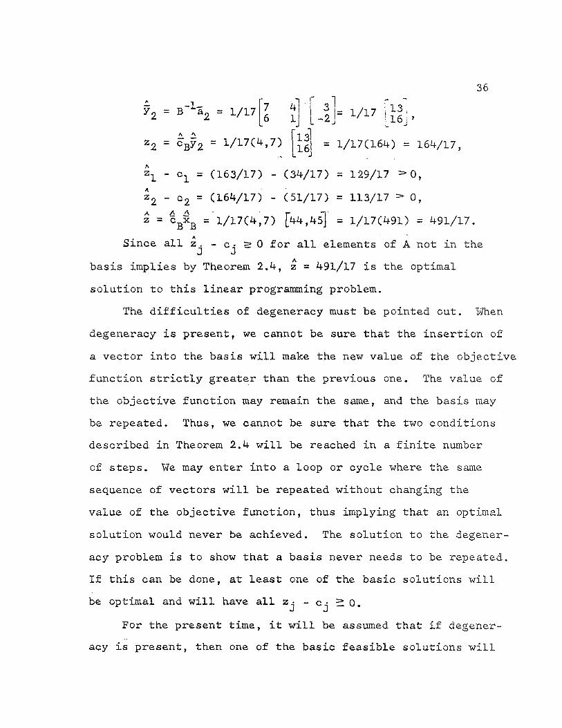
36
y2 = b_152 = 1/17H
z2 =
3 - 2
13 16
» 1/17 1 3 /J" 16
i -
1/17(164) = 164/17,
A Z
A
Z<
L - c]_ = (163/17) - (34/17) = 129/17 > 0,
2 = (164/17) - (51/17) = 113/17 > 0, - c A A
Z = cBxB = 1/17(4,7) [44,45] = 1/17(491) = 491/17.
Since all 2 . - c • s 0 for all elements of A not in the
basis implies by Theorem 2.4, z = 491/17 is the optimal
solution to this linear programming problem.
The difficulties of degeneracy must be pointed out. When
degeneracy is present, we cannot be sure that the insertion of
a vector into the basis will make the new value of the objective
function strictly greater than the previous one. The value of
the objective function may remain the same, and the basis may
be repeated. Thus, we cannot be sure that the two conditions
described in Theorem 2.4 will be reached in a finite number
of steps. We may enter into a loop or cycle where the same
sequence of vectors will be repeated without changing the
value of the objective function, thus implying that an optimal
solution would never be achieved. The solution to the degener-
acy problem is to show that a basis never needs to be repeated.
If this can be done, at least one of the basic solutions will
be optimal and will have all z - c^ SO.
For the present time, it will be assumed that if degener-
acy is present, then one of the basic feasible solutions will

37
be optimal. The degeneracy problem will be resolved by-
showing that a basis never needs to be repeated.
Although the optimal value of the objective function is
unique, the set of variables which yield this optimal value
need not be unique as shown in Chapter 1.
Theorem 2.5 If • • *, x^ are k different optimal
basic feasible solutions to a linear programming problem,
then any convex combination of 5c , • * *, is also an
optimal solution.
Proof: Consider any convex combination of these solutions: — _ k x = A uixi» ui-° Ci=l, •••, k), £ Uj. = 1.
i=l . i=i
Since each x^ 2 0 and u^ 0, then x 0. Since Ax^ = b, then
Ax = b which implies that "x is a feasible solution. If
z = max z = cx^ Ci=l, ***, k),
the value of the objective function for x is __k k
cx ££1 * * i"=l " \ j=l i^l
= C I uixi = X, = Z ai* = ® i ui = 2.
Hence, x is an optimal solution.
The preceding proof shows that if there are two or more
different optimal basic solutions, then there are an infinite
number of optimal solutions. But we do not need two or more
optimal basic solutions to have an infinite number of optimal
solutions, as is illustrated in Graph 1.3.
Theorem 2.6 If there exists an optimal basic feasible
solution to a linear programming problem; and, for some

38
not in the basis, Zj - cj = 0, y^j f: 0 for all i, then
^ (xg^ - Oyii)t>£ + Oa^ = b is also an optimal solution for i=l. any 9 > 0.
m
Proof: Let xBi^i = b be ^ e optimal basic feasible
solution. Then by adding and. subtracting 9§j, we obtain m _ _
X L XBibi + 8Sd " e &j = b'
m but -9a • = -9 V y - -b-. Hence by substitution,
J i=l J 1
m. _ _ .^C^Bi^i - 0yijbi> + Q*j = b,
or X.CxBi " i j ^ i + °*j = b* m £
i=l
Hence, the value of this solution is the same as that for the
optimal basic feasible solution. Therefore, the solution is
optimal.
If the set of variables which yields the optimal value
of the objective function is not unique, then there exist
alternative optima.
We shall now return to the geometric interpretation of
linear programming. The following theorem makes the connection
between basic feasible solutions and the extreme points of the
convex set of feasible solutions to Ax = b.
Theorem 2.7 Every basic feasible solution of a linear
programming problem is an extreme point of the convex set of
feasible solutions, and every extreme point is a basic feasible
solution to the set of constraints.
39
Proof: Suppose there exists a basic feasible solution
X to the set of constraints Ax = b. If the vector x is an
n-component vector, then it includes both zero and nonzero
variables. Number the variables so that "x = [xB,0j where
x-g = B~ -b. Now it must be shown that x is an extreme point.
To do this, we must show that there do not exist feasible
solutions xL, x2 different from x such that
x = Ax^ + (1-/1)52, 0 ^ ^ •L#
Divide the vectors and Xj so that
*1 ul'vl ' x2 = u2, v2
where u^, u2 are m-component vectors, and v^, v2 are (n-m)'
component vectors. Then
xfi= jIu + (l->2 )u2
0 = Jl v^ + Cl-^)v2.
Since A , (1-A ) =* 0, then v-, = = 0. Therefore,
X1 = Lul'°. , x2 = LU 2,°
which implies Ax^ = Bu^ = b, and Ax2 = Bu2 = b.
However, since the expression of the vector b is unique in
terms of the basic vectors, then Xg = u^ = u2, and x = = x2,
Therefore, there do not exist feasible solutions different
from x which implies x is an extreme point. Hence, any basic
feasible solution is an extreme point of the convex set of
feasible solutions.

40 ^ r
Now we must show that any extreme point x = xn
of the set of feasible solutions is a basic solution. To do
this, we shall prove that the vector associated with the
positive components of x* are linearly independent.
Suppose that k components of x* are nonzero. Number the
variables so that the first k components are nonzero. Then k __ 5] x±&± = b, i=l, •••, k. i=l
If the a^ are linearly independent, then they form a basic
solution. But suppose they are linearly dependent. Then k _ XJ iai = 0 ? where at least one JI . 0. Now consider i=l
c* = min (x^/ | & J ) , i / 0, i=l, • • -, k.
<=* is a positive number since x^ 0, so if we choose an £
such that 0 «= €" <=£*, then
xi + € ^i ^ °» and xi - e A i > 0, i=l, k.
Now define a n-component vector A. 0 which has X defined
above in the first k positions and zero in the last n-k
components. Let
x- = "x*. + €/l , and x2 = "x* - gjl .
By the discussion above, 2 0, x2 2 0, and AJI =0. Hence,
Ax-j_ = Ax + € A/i = Ax + 0 = b,
and Ax £ = Ax + € A A = Ax + 0 = b.
Therefore, , x2 are feasible solution different from x*.
Adding the preceding equations,
AX^ + AS 2 = 2Ax*,
or 5c* = (l/2)x^ + (1/2)x2»
Bat this contradicts the fact that x is an extreme point since
x* = 7\x + (1 - TOix^, where 7\ = 1/2.
Hence, the columns of A associated with the nonzero components
of any extreme point of the convex set of feasible solutions
must be linearly independent. Since there are only m equations,
there cannot be more than m linearly independent columns of A;
and therefore, an extreme point cannot have more than m positive
components. If an extreme point has less than m positive com-
ponents, then it is a degenerate basic solution since m-k
columns of A are added at the zero level. Hence, every extreme
point is a basic feasible solution to the set of constraints.
The reader may have wondered throughout the above dis-
cussion why we have restricted our attention to changing only
a single vector in the basis at each iteration. No way has
been found to change more than one vector at a time that is
less time consuming than changing only a single vector. We
shall point out some of the problems that occur when two
vectors are involved. We must first derive a method by which
the new vectors replace the old ones, and there is still a
basic feasible solution. In this method the two vectors which
are to be inserted must be linearly independent. Also, we must
have a special case in the method which allows us to insert only
one vector into the basis. Therefore, this type of combination
could become very involved and. cause considerable calculations.

42
Also, the question may have risen concerning the linear
programming problem AS = b, where b = 0. Suppose B is a basis
of A. Then there, are two cases which we must consider: 1) B
is singular, and 2) B is nonsingular. Suppose B is singular.
Then we have a contradiction, for B is therefore not a basis.
Hence, B must be nonsingular, and B--'- exists. Therefore,
XB = = = B~ "0 = 0, or a basic feasible solution
is Xg = o. It is immediately obvious that the objective
function z cannot be improved since min z = max z = 0. Hence,
since the trivial solution is the only basic feasible solution,
this type of linear programming problem is meaningless.
Theorem 2.7 Let there be given a linear programming
problem Ax = b, x 2 0, max z = ex. If x* is an optimal basic
solution to this problem, then x is also an optimal basic
solution to a problem whose price vector is c* = A c, A > 0.
Also, x is not necessarily an optimal basic solution to a / \
problem whose price vector is c = c + i 1, A / 0.
Proof: In the original problem, for all yi ^ 0, ZA - c• >0 J J 5
if an optimal basic solution exists. Hence, we wish to show
Zj - Cj -0, for all y- c 0. Zj cj = cByj - cj = ^cByj - Acj
- ^(cByj - Cj) = - cj) > o.
Therefore, zj - Cj >0 which implies x* is an optimal basic
solution, to the problem whose price vector is c*.

43
jL _ i
If the price vector c = c + / 1 is used, then
Zj ~ = ~ Cj = CcB •+ A l)yj - Cj - J( 1 = V j yj /< i - oj - A i
= cByj - cj + (yj^ 1 - /} 1)
= zj - cj + A iCyj - 1)
Case I: If A ^ 0, then we have increased the ob-
jective function by /llCyj - I); and therefore, x is not an
optimal basic solution.
Case II: If A > 0, then we may not have reached an
optimal basic solution; for if c^ - z± S: A I(y^ -1), then J J J
zj - Cj + A ICyj - 1) - 0. But if Cj - Zj <" A ICyj - I),
then zj - cj + A - 3-) > 0 which implies we have reached
an optimal solution.
Therefore, if the price vector c = c + A I is used,
then x is not necessarily an optimal basic solution.
It should, be noted that all of the theorems in this
section could be proved similiarly if z is to be minimized.
Therefore, the simplex method is satisfactory to maximize or
minimize the objective function.
CHAPTER BIBLIOGRAPHY
I. Hadley, George, Linear Programming, Reading, Massachusetts, Addison-Wesley Publishing Company, Inc., 1962.

CHAPTER III
COMPUTATIONAL ASPECTS OF THE SIMPLEX METHOD
In the preceding chapter we have shown how to solve
a linear programming problem by use of the simplex method,
given a feasible solution to the problem; but this procedure
requires many calculations. Now we would like to show how
some of these computations can be avoided (1, pp. 108-144).
We wish to solve the linear programming problem
Ax = b, x - 0, max z = cx, where A is an m x m matrix. The
following discussion shall be limited to maximizing the ob-
jective function, but it is also true for minimizing.
Given any basic feasible, but not optimal, solution to
this linear programming problem, the theory developed in the
preceding chapter indicated how to obtain a new basic solution
with the new objective function improved or at least equal to
the old one; or it may show that an unbounded solution exists.
In this process we were forced to calculate and use the y •
and Zj - Cj for the vectors not in the basic solution in order
to determine the new basic solution. Suppose there is not an
unbounded solution, or Zj - cj <0, where at least one
y^j > 0, i=l, *••, m. Then we can insert any vector "aj with
Zj - Cj < 0 and obtain the new basic feasible solution. Of
45
kS
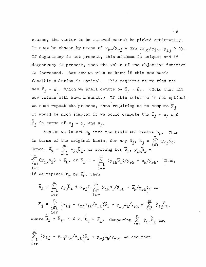
course, the vector to be removed cannot be picked, arbitrarily.
It must be chosen by means of Xg/y . = min (x-g./y. . y. . >0). XJ X. X. J X, J
If degeneracy is not present, this minimum is unique; and if
degeneracy is present, then the value of the objective function
is increased. But now we wish to know if this new basic
feasible solution is optimal. This requires us to find the
new z. - c., which we shall denote by z. - A.. (Note that all •J 3 *J J
new values will have a carat.) If this solution is not optimal, A
we must repeat the process, thus requiring us to compute y^.
It would be much simpler if we could compute the - c• and A y. in terms of z. - c. and f-. J J J J
Assume we insert a^ into the basis and remove br. Then
_ m — in terms of the original basis, for any a., a- = ^ y • -b •.
m _ i = I 13 1
Hence, ak = ]T yik^i, or solving for br, yrkbr = m — __ m A j ^ i k V + V o r b
r = " .£ ^ik^i^/yrk + V y r k " T h u s'
itr i^r if we replace fc>r by I"k, then
_ m _ m __ aj = Al y U b i + y i k V y r k + V W - o r
ifr i#-r
— <r-< — _ m £ aj ~ ^yij ~ yrjyik/yrk^bi * yrjal/yrk = yijbi'
i^r £ — . — - m *
where bj. - b.^ i r, br = a^. Comparing 2 9,- jb. and i~l J
m
i?i ( 7 i j ~ yrjyil/yrk)5i * yrjal/yrk' W e s e e t h a t
i*r
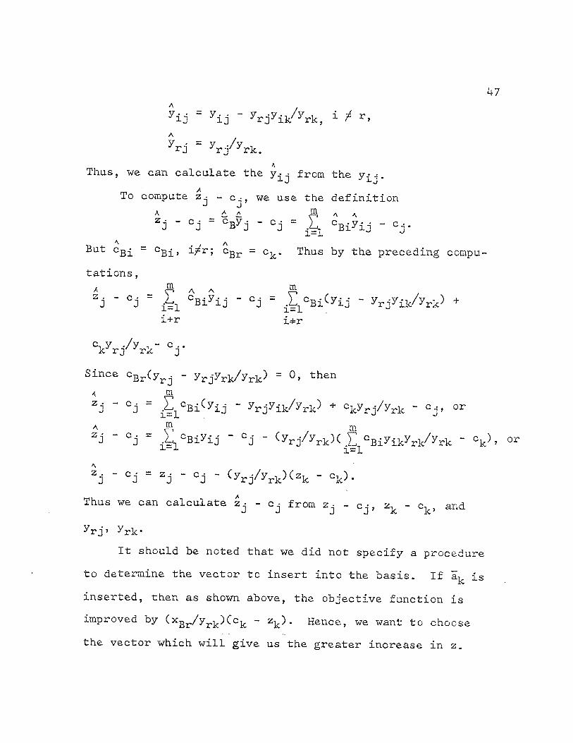
47
yij yij " yrj^ik/^rk, ^ r>
yrj ~ yrj/yrk. A
Thus, we can calculate the from, the yij.
To compute Zj - c-, we use the definition A _ 6. £. A A zj - cj - °Byj - cj = .1 cBiyij - °j-
But c g i = cB£( i/r; c B r = ck. Thus by the preceding compu-
tations,
* _ V* A A
Zj ~ CJ ~ CBiyij " cj = L. cBi^yij ~ yrjyik/yrk^ * i=l J J i=l i+r i^r
c. y ./y - c .. k rj rk j
Since cBr(yrj - yrj-yrk/yrk) = 0, then
a m Z3 ' °j = - i k / ^ * ckyrj/yrk - cj' o r
A _ <T' / m
Zj " °J ~ " °j - r j/yrkXX cBiyikyrl/yrk " ck ) > o r 1 = 1
Zj - Oj = Zj - Cj - Cyrj/yrk)(zk - ck).
Thus we can calculate - c^ from zj - Cj, zk - ck, and
yrj» yrk-
It should be noted that we did not specify a procedure
to determine the vector to insert into the basis. If ak is
inserted, then as shown above, the objective function is
improved by ^xgr/yr]<;)Ccjc - z .). Hence, we want to choose
the vector which will give us the greater increase in z.
48
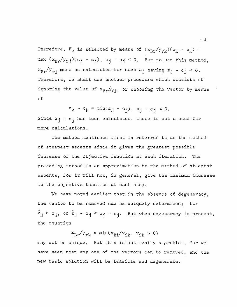
Therefore, a . is selected by means of (x^/y^Kc^. - z .) =
max CxBr/yrj)Ccj - Zj) , Zj - Cj < 0. But to use this method,
xBr/yrj m u s t b e calculated for each a.j having zj - cj •< 0.
Therefore, we shall use another procedure which consists of
ignoring the value of o r choosing the vector by means
of
zk - ck = min(zj - cj), zj - cj < 0.
Since Zj - Cj has been calculated, there is not a need for
more calculations.
The method mentioned first is referred to as the method
of steepest ascents since it gives the greatest possible
increase of the objective function at each iteration. The
preceding method is an approximation to the method of steepest
ascents, for it will not, in general, give the maximum increase
in the objective function at each step.
We have noted earlier that in the absence of degeneracy,
the vector to be removed can be uniquely determined; for A A
2j > Zj, or Zj - Cj ^ Zj - Cj. But when degeneracy is present,
the equation xBr^^rk ~ m^n^xBi/^ik' ^ik > ^
may not be unique, But this is not really a problem, for we
have seen that any one of the vectors can be removed, and the
new basic solution will be feasible and degenerate.

49
We shall now continue with some further developments
of the transformation formulas. In the simplex method, only
one single vector is changed, in the basis matrix at each
iteration. Therefore, it would be advantageous if we could
keep from calculating a new inverse every iteration.
Suppose we begin with a basic feasible solution charac-
terized by the basis matrix B = (b^, b ). Further-
more, suppose that Er is to be removed and. is to be replaced,
by a .. If the inverse of the original matrix B is known, then
- -Xi-" -1_
xB - B b. y^ = B aj, j=l, n. If the new basis matrix A A-l - _ A - 1 -
is known, then x_ = B b, y. = B a. are the new values of B J J xB and y .. Since B and. B are two bases for En, then is J '
_ m _ A
ak = an<3' B will be nonsingular if and only if
yrk ^ 0- Assuming this is the case, then 5k = yikBl + + yr,kBr + ••• + y ^ V °r
^rk^r "''lie0! ^r-l,k^r-l + ak ~ *** -
°r br = (-yik/y^Bj. - ... - y r_ 1 > kS r_]Ark - iTk/yrk -
yr+L,k^r+l^rk ~ ~ ' o r ~
where h = [-yik/yrk - - y r_ 1 ) k/y r k + i/yrk - y r + l j k/y r k
- *•" ~ ymk/^rk] " H e n c e> B = BE, where E differs from the
identity matrix only in the r-th column, i.e., E =
(£]_, •••, er_]_, "E,er+L, *•*» Therefore, B-1 = EB"1.
Now we can write
— _i - - — i _ xB = EB b = Exb; y . = EB a - = Ey ..
50
When these two equations are expanded., we obtain simply
xBi = xBi ~ xBr^ik//'yrk'
xBr ~ "^Br^rk'
and y ± j = y ± 6 - yrjyik/yrk, tfr,
yr j j/^rk'
which are the same as derived at the beginning of this
chapter.
The discussion thus far has been based on the assumption
that we had an initial basic feasible solution to the linear
programming problem. If we can develop a method of finding
an initial basic feasible solution, then we shall have a
computational procedure which will in theory solve any linear
programming problem.
We shall first consider the case where a basic feasible
solution can be immediately determined. Suppose each of the
constraints contain the inequality - . Then we must intro-
duce a slack variable to each constraint. The matrix A for
the set of constraints Ax = b has the form A = (R,I), where
R is the Sj associated with the true variables and 1 with the
slack variables. I is then an m-th order identity matrix, for
the column corresponding to the slack variable r+-]_ is e^. If
we write x = [xr, xg"j, where "xr contains the real variables
and xg the slack variables, then (R,I) xr, ~xs~| = b, or by
51
setting xr = 0, Ixs = b. Here we have a basic solution
containing only the slack variables, and it is feasible
since x-r, = b and b - 0. Therefore, since B = I, then JO yj = B" 1^ = laj = aj, j=l, •••, n, and
o E = 0 .
Hence, - a. = pByj - a. = -Cj,
z = c x = 0. B B
As readily seen, this basic feasible solution is especially
easy to work with since no further computations are necessary
to obtain the quantities xfi, z, yj, Zj - cj. Hence, we can
use the simplex method without difficulty.
Above we have shown that it is simple to find a basic
feasible solution if slack variables are present in each of
the constraints. However, this procedure can be used when-
ever an m x m identity matrix appears in A. Of course, if
the columns of the identity matrix are not slack variables,
then Xg, yj, Cg, and Zj - cj may not be what was stated
above; but they can be computed easily from the original
equations.
Now we must consider the cases where no identity matrix
appears in A. This will occur almost always when some con-
straints do not require slack or surplus variables. Under
these conditions, there is usually no easy way of finding
an initial basic feasible solution.

52
Suppose we always begin with an identity matrix for the
initial basis matrix. Instead of the original set of con-
straints Ax = "b, consider the new constraint equations
Ax + Ixa = (A,I) ^XjXgJ = b.
We have augmented, the original constants by adding m additional
variables which shall be called the artificial variables.
The columns corresponding to the artificial variables are e^,
which are called the artificial vector. Now we have immedi-
ately a basic feasible solution to the problem, namely
x a = b, x = 0. But this is not a feasible solution to the
set of constraints. The artificial variables must vanish,
x a = 0, so that Ax + Ixa = Ax = b. Thus, we must find a
method to move xa = b to x a =0. A very interesting obser-
vation can now be made. We can use the simplex method itself
to insert columns a • of A into the identity matrix and. drive
the artificial variables to zero. If this is done, then we
will have a basic feasible solution to the original constraints
and can then continue to find an optimal basic feasible solution,
if one exists.
Since the vector to be inserted into the basis is deter-
mined by Zj - cj, and we do not have a Cj for the artificial
variables, then we can assign a price to these variables which
are so unfavorable that the objective function can be improved
as long as any artificial variable remains in the basis at the
positive level. Hence, if z is to be maximized, we can assign
53
a very large negative price to each of the artificial vari-
ables. Let ca£ be the price corresponding to the artificial
variable xa^. Then
cai = ^ > if z is t 0 maximized,
cai = M, M > 0, if z is to be minimized..
Therefore, given any linear programming problem Ax = "b, x — 0,
max z = cx, then we can begin our computations with the aug-
mented problem Ax * Ixa = b, x £ 0, max z s ox - Mxa, and
find immediately the basic feasible solution xa = b. This
method of finding a basic feasible solution was first sug-
gested by Gharnes.
The following example will illustrate the introduction
of artificial variables into a linear programming problem.
5x|_ - 2x2 + x3 ~ — 2,
6xl + x2 ~ 5x3 " 3 x4 - 5'
-x^ + i+x2 + 3x3 + 7X4 > 6,
all Xj 2. 0,
min z = 3x, + 4x2 + X3 + 6x^.
After adding the surplus variables, we obtain
5x- + CM
X CM 1 X3 - 3xh - x5 = 2,
6Xl + x 2 - 5x3 - 3x^ - x6 : = 5,
"X1 +4X2 + 3X3 + 7x^ -x7 = = 6.
Since no vector in our linear programming problem is equal
to a unit vector, it is necessary to add. three artificial
variables xa^ = e^, x a 2 = e2, and. xa^ = "e . Therefore,
54
5x, •1 " 2 x2 + x3 - —It
6x^ + X2 - 5x^ - 3x^ - xg
-x _ + 4x2 + 3x^ + 7x^ - Xy
rain z = 3x]_ + 4x£ + X3 + 6x^ + Mxa]_ + Mxa£ + M xa3
where M is very large.
3x, xt + x, Ll
+ xa2 = 5,
+ x a 3 = 6,
Choose B 1 0 0 0 1 0 0 0 1
, then B
2,5,6
-1 B.
= B-Ib
yj = B-^j, SO yL =
1?-5,3
Vl± = _ -3, - 3, 7 , y^
0,0,-1
5,6,-l] ,
-1,0,0
^2
ye =
,1,^], •2 •
0,-1,0
^3
y-7
z . J
- c . = J
CB yj " cj' w h e r e CB = (M,M,M)
Z1 - cL = 5,6,-l] -3 = 10M - 3
z2 C2 = (M,M,M) -2,1,4 _!+ = 3M - 4,
z3 - c3 = , 1,-5,3 -1 = -M - 1,
z4 - c 4 = (M,M,M) | -3 -3 7 L ' ' .
-6 = M - 6,
z5 " c5 = rl,0,0_ = • -M,
z6 " c6 = „ 0,-1,0 = • -M,
z7 - c7 = _ 0,0,-1 = • -M.
Since z is to be minimized, and. M has been chosen very large,
then aL has the largest Zj- - Cj > 0. Hence, aL shall be
inserted into the basis.
55
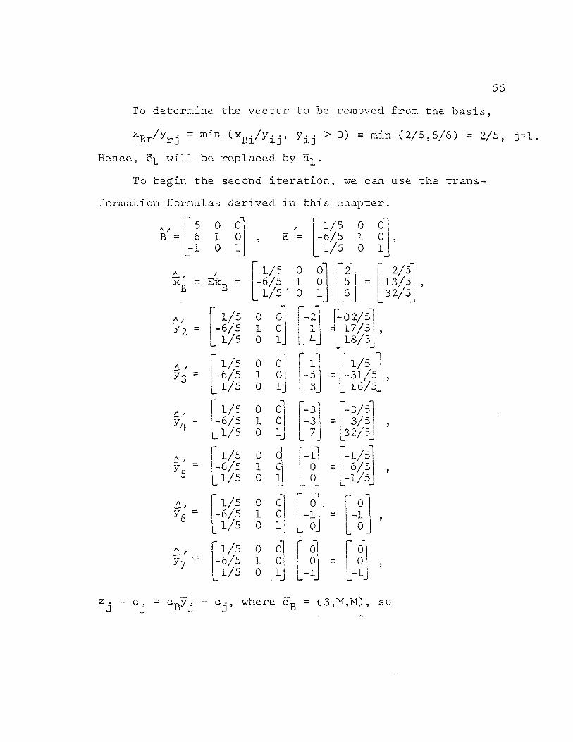
To determine the vector to be removed, from the basis,
xBr/yrj = m i n ^xBi/yij» yij > 0 ) = m i n C2/5,5/6) = 2/5, j=l,
Hence, e^ will be replaced by a" *
To begin the second, iteration, we can use the trans-
formation formulas derived, in this chapter.
/
B 5 0 0 6 1 0
- 1 0 1
B = E xB
y 2
y3 =
a/ y4 =
A_
yt
A
y7
/
E = 1/5 0 0 -6/5 1 0 1/5 0 1
2 2/5 5 = 13/5 6 32/5
1/5 0 0 -6/5 1 0 _ 1/5 0 1_
1/5 0 0 -6/5 1 0 _1/5 0 1
1/5 0 0 -6/5 1 0 _1/5 0 1
1/5 0 0 -6/5 1 0 _1/5 0 1
" 1/5 0 0 -6/5 1 0 1/5 0 1
1/5 0 0 -6/5 1 0 1/5 0 1
- 2
1 -5 _ 3v
-3 -3 7
" - 1
0 ^ 0
0 -1 -0
t
0 0 -1
1 02/5 17/5 18/5
1/5 -31/5 16/5
-3/5 3/5 32/5
L.
-1/5 6/5 -1/5
" o' -1 0
" 0 0 -1
z . - c . J 3
cByj " °j' w h e r e cb = C3,M,M), so

56
A /
z2 - c 2 - ( 3 ,M,M) '-2/5, 17/5, 18/5 - i+ = 7M - 26/5,
A / Z3 " C3 = C3,M,M) ~ 1/5, -31/5, 16/5 - 1 = 3M - 2/5,
A / Z k
- = C3,M,M) L~3/5'
3/5, 32/5] | - 6 = 7M - 39/5,
*• / z5 - c 5 = C3,M,M) [-1/5, 6/5, -1/5 = M - 3/5,
A/ z6
c6 = C3,M,M) 0,-1 f
' ° = -M,
A / z 7
- cy = C3,M,M) [ o , o , -1 = -M.
Hence, shall be inserted, into the basis.
To determine the vector to be removed from the basis,
A • / A / . A / A • A/ XBr / yrj = m l n C* B:/
y2j' y2j " 0 3
= minCl3/l7,32/18) = 13/17, j=2.
Therefore, will be replaced by a^.
To begin the third iteration,
A
B" 5 6
-1
-2 0 1 0 k 1
E" = 1 2/17 0 0 5/17 0 0 -18/17 1
_ H _ I
Xg = E"x so
X B
y<>
1 2/17 0 0 5/17 0 _0 -18/17 1
1 2/17 0* 0 5/17 0 ,0 -18/17 1
1 2/17 0 0 5/17 0 0 -18/17 1
1 2/17 0~ 0 5/17 0 0 -18/17 1
2/5 13/5 _32/5
= 12/17 13/17 _62/l7_
1/5 -31/5 l6/5_
= -9/17
-31/17 166/17
'-3/51
3/5 32/5_
= -9/17 3/17
_98/18_
"-1/5 6/5
-1/5 .
' -1/17]
- 2 b / \ l \
57
* t .
y 6 =
y7 =
1 0 0
1 0 0
f 0 i -1
0
) r~ *1 r 0
) 0 -1
-2/17 -5/17 18/17
0 0 -1
A f t Zj A „ Z3 A i t 2, 4
- C r tlAH
5 B y j Cj, where cB
A 11 Z
a n 2 A n
2
C3,4,M); so
cr. = (3,4,10 f-9/17,-31/17,166/17] - 1 = (166/17)M - 168/17, or
- C4 = C3,4,M) [-9/17,3/17,98/17] - 6 = (98/l7)M - 117/17,
5 - c5 = (3,4,M) [-1/17,6/17,-25/17]= -C25/17)M + 11/17,
6 - c6 = (3,4,M) [-2/17,-5/17,18/17]= (18/17)M - 29/17,
7 - c? = C3,4,M) [0,0,-l] = -M.
Hence, a3 shall be inserted, into the basis.
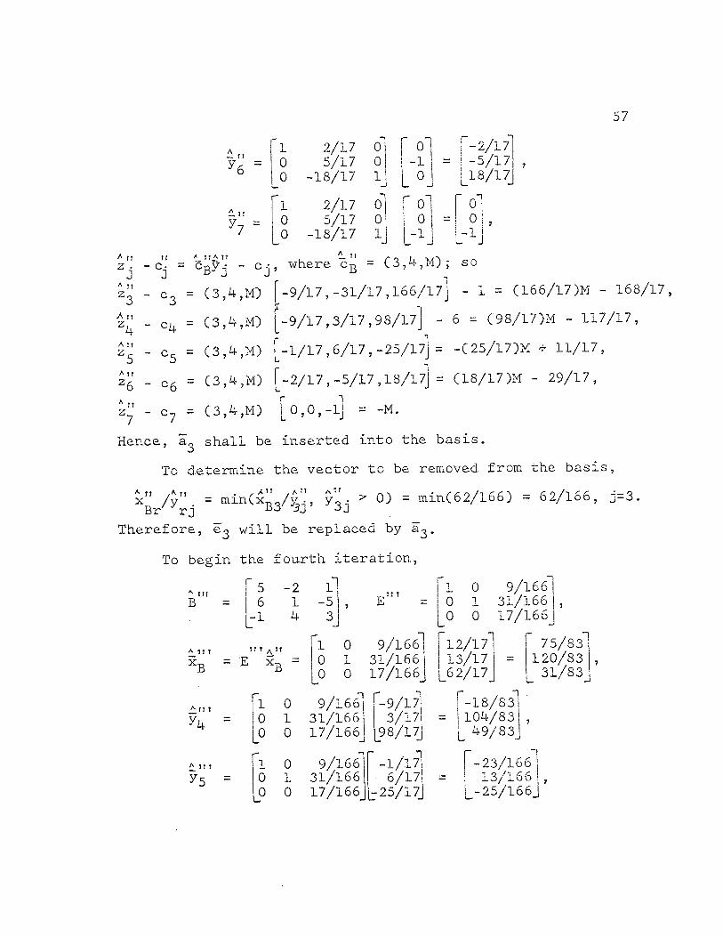
To determine the vector to be removed, from the basis,
x" /J" = min(x" /%!, y" ^ 0) = min(62/l66) = 62/166, j=3. Br r j B3'J33' 3j
Therefore, eg will be replaced by a^.
To begin the fourth iteration,
B
T
XB
At? t y;,
A tr t ^5
5 -2 6 1 -1 4
A . "
= E xB
E
1 0 9/166 0 1 31/166 0 0 17/166
1 0 9/166 0 1 31/166 0 0 17/166
12/17 13/17 6 2/17
7 5 / 8 3 1 2 0 / 8 3 ,
3 1 / 8 3
1 0 9/166 0 1 31/166 0 0 17/166
f -9 /17 1 - 1 8 / 8 3 3 /17 = 104 /83
98 /17 4 9 / 8 3
1 0 9/166 -1/17 -23/166 0 1 31/166 6/17 13/166 0
W 0 17/166 -25/17 -25/166

58
A J T | ^6 =
A j ! T
y 7 =
1 0 9/166 0 1 31/166 0 0 17/166
"l 0 9/166 0 1 31/166 0 0 17/166
-2/17 -5/83 -5/17 = -8/83 , 18/17 9/83
0 0 -1
-9/166 -31/166 -17/166
A i i :
2 . 3
L , 1 h »
c . = J V. A l l !
Z4 " C4 : A T ! I
Z5 °5 A »» »
Z6 " c6 A. I T t
z7 -c7
K 11 T
c., where c J B — (3,4,1); so
= (3,4,1) [-18/83,104/83,49/83] -6 =-87/83,
''7 ~ °5 = C 3' 4' L ) [-23/166,13/166,-25/166] = -42/166,
c6 = (3,4,1) [-5/83,-8/83,9/83] = -38/83,
(3,4,1) r_9/i66,-31/166,-17/166] =-178/166.
A H I
Since all z- - c• £ 0 for all columns of A not in the basis, J J
we have obtained, the optimal solution for min z = 3x-j_ + 4x2 +
x3 + 6x4, or z = 3(75/83) + 4(120/83) + 31/83 = 736/83.
Now we shall discuss a problem that has been avoided
throughout this discussion, that of redundancy and. inconsistency.
We have always assumed r(A) = r(A^) = m; so that we knew a
basic feasible solution exists. ¥henever we begin with an
identity matrix, which is composed of true variables, slack
variables, and/or artificial variables, then it is obvious
. that r(A) = r(A^) = m, which implies that a basic feasible
solution exists. Hence, the assumption in the discussion of
the simplex method is valid. Thus, we wish to show that if
we start with the augmented system whose initial basic feasible
solution consists entirely or in part of artificial variables,
then we can determine by means of the simplex method, if the

59
original constraint equations are consistent and. if any of
them is redundant. We shall assume the optimality criterion
is satisfied, and there exist no unbounded solutions.
There are three cases which we must consider: 1) There
are no artificial variables in the basis; 2) One or more
artificial variables are in the basis at the zero level;
3) One or more artificial variables are in the basis at the
positive level. Therefore, we shall use three theorems to
show these three cases.
Theorem 3.1 If no artificial vectors appear in the
basis, and the optimality criterion is satisfied, then the
solution is an optimal basic feasible solution to the given
problem, and. the constraints are consistent and. none of the
equations is redundant.
Proof: Since no artificial variables appear in the
basis, and. the optimality criterion is satisfied, then we
have found an optimal basic feasible solution. Therefore,
the constraint equations are consistent, and none are re-
dundant .
Theorem 3.2 If one or more artificial vectors appear
in the basis at the zero level, and the optimality criterion
is satisfied, then the solution is an optimal basic feasible
solution to the given problem, and. the constraint equations
are consistent, but redundancy may exist.
60
Proof: Since all the artificial vectors are at the
zero level, we have a feasible solution to the original
constraints. Therefore, the constraint equations are
consistent.
But two cases arise in the question of redundancy.
Case I: Suppose y — / 0 for some and for i
corresponding to a column of B which contains an artificial
vector. Then as shown in Theorem 2.2, the artificial vector
can be removed and replaced by a.. Since the artificial
variable was at the zero level, then aj will enter the basis
at the zero level, thus implying the new basic solution is
feasible; and the value of the objective function will be
unchanged. If more than one artificial variable is present
in the basis, then we can continue this process until all
the artificial vectors are removed or until for all the
artificial variables, y^j = 0, which is considered in Case
II. Thus we have obtained a degenerate optimal basic feasible
solution containing only the true variables. Therefore, none
of the constraints are redundant.
Case II: Suppose y — = 0 for all a. and all i corres-
ponding to the columns of B containing the artificial vectors.
Then we cannot maintain a basic solution if an artificial
vector is replaced by some aj. Since all the artificial
vectors are in the basis at the zero level, then all the

61
columns of A can be written as a linear combination of the
columns of A which are in the basis. If there are k arti-
ficial vectors in the basis, then A can be written as a
linear combination of the m-k linearly independent columns
of A in the basis. Therefore, r(A) = m-k, or k of the original
constraints are redundant.
Theorem 3.3 If one or more artificial vectors appear in
the basis at the positive level, and the optimality criterion
is satisfied, then the original problem has no feasible solution
either because the constraints are inconsistent or because the
solutions are not feasible.
Proof: There are only two cases which we must consider,
namely y^j > 0, and. y^j = 0; for if y ^ ^ 0, then we have not
reached the optimal solution.
Case I: Suppose there exists a y•- > 0 for some a-; X J J
and for i corresponding to a column of B which contains an
artificial vector. If we insert aj into the basis, then the
new solution may or may not be feasible. But it should be
noted that if only one artificial vector is in the basis at
the positive level, such a situation cannot occur since
zj - cj = -Myj_j + cj < 0, and the optimality criterion would
not be satisfied. Therefore, we shall continue the above
procedure until all the artificial vectors are removed., which
yields a basic but not feasible solution, or y— :£ 0 for all
and i corresponding to a column of B which contains an

62
artificial vector. The case of y — = 0 for some aj is
considered in Case II, so suppose y — < 0 for some a j.
Then we can replace the artificial vector by aj; but
since y^j <0, aj will enter the basis at the negative
level. Therefore, if this process is continued, until all
the artificial vectors are removed, then we have obtained,
a basic solution which is not feasible.
Case II: Suppose there exists a y^ • = 0 for some
aj and for some i corresponding to a column of B which
contains an artificial vector. Since the true variables can
be written as a linear combination of the k true variables in
the basis, then r(A) = k. But since the artificial vectors
are needed in the basis to write b as a linear combination
of the basis, then rCA^) > k. Therefore, r(A) / ^CA^) which
implies the constraints are inconsistent.
As noted in the development of the simplex method, it
is sometimes possible to determine which constraints are
redundant. Such is the case when y^j = 0 for all aj and. all
i corresponding to the columns of B containing artificial
vectors at the zero level.
Suppose that only one artificial vector e!rL appears in
column s of the basis at the zero level.. Then r(A^) =
rCAji^) = m since B is a basis with only one artificial vector,
which implies rCA) = m-1. Denote the rows of A by "a and the
63
rows of (A,eh) by (a^Q), i^h, (ah,l), i=h. Since r(A) = m-1,
then the are linearly dependent, or there exist not all m
zero such that ^ iai = ^ow w e nee(l to show that ^ 0. i=l
Assume by way of contradiction that c>$ = 0. Since
rCAje^) = m, then by the definition of linear independence,
the only satisfying m f iiCa^O) + ^hCah,l) = 0 1=1 i*h
are = 0, i=l, ***, m. But if we set A = cK then m £ ^Caj^.o) + « hcs h,i) = o 1=1 i^h
which is a contradiction. If we apply this reasoning step
by step, and if a number of artificial vectors e^ appear in
the basis at the zero level and the corresponding y — = 0
for all aj, then for each i the i-th constraint in the origi-
nal system, of equations is redundant and can be dropped.
Throughout this entire discussion we have treated maximum
and minimum problems separately, but now we wish to show that
one is a transformation of the other.
• Theorem 3.4 Any minimization problem can be converted
to a maximization problem by a transformation, and vice versa.
Proof: Suppose there exists a function of n variables,
xn), and let f" be the minimum value of f at points
x in some closed region of E .
6k
By definition of an absolute minimum, for every point
x in the region
f*- f * 0,
or by multiplying by -1,
C-f*) - C-f) £ 0.
But this is the definition of an absolute maximuai
C-f) = max C-f),
and -f takes on its maximum value at x". Hence,
min f = f* = -C-f*) = -maxC-f),
or min f = -maxC-f),
and the minimum of f and the maximum of -f are taken at the
same points. Therefore,
min z = -maxC-z) = -maxC-cx) = -max(-c)x.
If the function to be maximized is z = C-c)x, then min z =
-max z*. Finally, to convert a linear programming problem
in which z is to minimized, into a maximization problem, it
is only necessary to change the sign of every price.
Now we need to show that the change of sign of the prices
reverses the criteria for selecting the vector to enter the
basis and. the optimality criteria.
If a minimum has been reached, by means of the simplex
method, then Zj - Cj = cgyj - cj - 0 for all j. But we
replaced Cj by -cj to convert the problem to a maximization
problem, so -Cgyj - C-Cj) 2 0 for all j, which is precisely

65
the optimality criterion for a maximization problem. Simi-
larly, the vector to be chosen to enter the basis in a
minimization problem is
2k - ck = max(Zj - cj), Zj - Cj >0.
If we replace cjj by -cn-, we obtain
~zk " C-ck) = rain | - Z j - C-c^o]
which is the same criterion for choosing the vector to enter
the basis in a maximization problem. Therefore, the vectors
will enter the basis in the same sequence whether the problem
is treated as a maximization or a minimization problem.
Hence, we may solve only maximization linear programming
problems by merely changing the sign of the prices on a mini-
zation problem.
CHAPTER BIBLIOGRAPHY
I. Hadley, George, "Linear Programming, Reading, Massachusetts, Addison-Wesley Publishing Company, Inc., 1962.
66

BIBLIOGRAPHY
1. Hadley, George, Linear Algebra, Reading, Massachusetts, Addison-Wesley Publishing Company, Inc., 1961.
2. Hadley, George, Linear Programming, Reading, Massachusetts, Addison-Wesley Publishing Company, Inc., 1962.
67