linear programming modelling
TRANSCRIPT
R. Lahdelma
Linear Programming Modelling
Risto Lahdelma Aalto University
Energy Technology Otakaari 4, 02150 Espoo, Finland

R. Lahdelma
Contents
• Optimization modelling
• Mathematical programming models
• Linear programming
– LP model
– Formulation
– Sample energy models
– Graphical representation
– Solving LP models
• Basic solutions
• Simplex algorithm
– Combined heat and power modelling

R. Lahdelma
Optimization modelling
• The problem is defined in implicitly terms of
– an Objective function to minimize of maximize
– by choosing optimal values for decision variables
– subject to constraints
• Optimization software solves the problem automatically
– This approach is a dramatically different from explicit (simulation)
models where the result is obtained by applying some formulas in
given order
• Most common optimization model types:
– Linear Programming (LP) problem
– Mixed Integer Linear Programming (MILP) problem

R. Lahdelma
Optimization problem example
• Sample problem with two variables
min x12 + x2
2
s.t.
x1 + x2 3
x2 0
x1, x2R
• In a two-dimensional case the problem can be illustrated and solved graphically – Constraints define the feasible region in the plane
– Level curves of the objective function show the height of the terrain

R. Lahdelma
Optimization problem example
– Constraints define the feasible region in the plane
– Level curves of the objective function show the height of the terrain
-1
-0.5
0
0.5
1
1.5
2
2.5
3
3.5
4
-3 -2 -1 0 1 2 3 4
x1+x2=3
Z=1
Z=4.5
min Z = x12 + x22
(1.5, 1.5)
infeasible x1+x2<3 feasible x1+x2>=3
infeasible x2<0
feasible x2>=0

R. Lahdelma
General mathematical optimization
problem Find values for decision variables x that minimize or maximize the objective function f(x) subject to constraints:
min f(x) (objective function)
subject to
h(x) = 0 (vector of equality constraints)
g(x) ≤ 0 (vector of inequality constraints)
xRn (or xNn) (vector of decision variables)
If domain of x is Rn, it is a continuous optimization problem
If all xi are integers, it is an integer optimization problem
A mixed integer problem contains both integer and real xi
R. Lahdelma
Properties of optimization problems
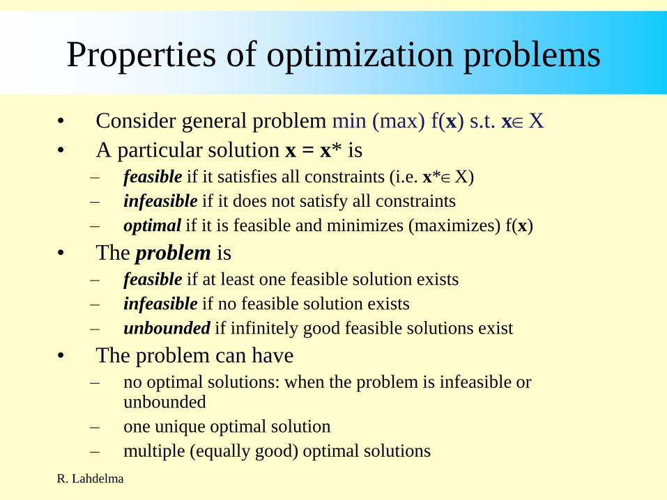
• Consider general problem min (max) f(x) s.t. xX
• A particular solution x = x* is
– feasible if it satisfies all constraints (i.e. x*X)
– infeasible if it does not satisfy all constraints
– optimal if it is feasible and minimizes (maximizes) f(x)
• The problem is
– feasible if at least one feasible solution exists
– infeasible if no feasible solution exists
– unbounded if infinitely good feasible solutions exist
• The problem can have
– no optimal solutions: when the problem is infeasible or unbounded
– one unique optimal solution
– multiple (equally good) optimal solutions

R. Lahdelma
Optimization model transformations
• Transformations
– min f(x) = -max -f(x);
– max f(x) = -min -f(x)
– g(x) 0 -g(x) 0
– g(x) = 0 g(x) 0 g(x) 0
– g(x) 0 g(x) + s2 = 0 where s is an unconstrained real variable
• Constrained problem can be transformed into unconstrained by augmenting objective with a penalty term, i.e. a barrier function
– min f(x) s.t. g(x) 0 min f(x)+Mmax{g(x),0} • M is a big positive number

R. Lahdelma
Optimization model types
• Depending on the structure of the objective function and constraints, optimization models can be classified in different ways – Single variable and multiple variables
– Continuous, discrete or mixed integer problems • Decision variables are continuous, binary (0/1), general
integers, or mixed
• Integer programming, mixed integer programming
– Unconstrained and constrained problems
– Convex and non-convex problems • Linear, quadratic and nonlinear problems
– Single objective and multi-objective problems • f(x) is a vector of objective functions

R. Lahdelma
Optimization model types – Exampes
• Sizing of ground source heat pump
– Single objective (minimize life-cycle costs)
– Single continuous variable (size of pump)
– Constrained non-linear convex problem
• Unit commitment of power plants
– Single objective (maximize profit)
– Multiple variables of mixed types
– Constrained non-convex problem
• Investment in new production technology
– Multiple objectives (economic, environmental, policy, …)
– Multiple discrete (binary) variables
– Constrained or unconstrained problem

R. Lahdelma
Solving optimization problems
• To solve problems it is necessary to understand the different problem types and their properties – There is no universal way to find the optimum or even
a feasible solution to an arbitrary problem
– Different solution algorithms are required for different problem types
• Most important is to determine if the optimization problem is convex or not!
– Convex problem = minimize convex objective function in a convex region
– Convex problem: relatively easy
– Non-convex problem: potentially very hard

R. Lahdelma
Impossible to solve non-convex model
• Consider max/min f(x)=sin(x)*sin(ax) – Each factor has max/min at +1/-1
– If the peaks and valleys coincide then f(x)=+1 or -1
– If a is chosen properly, peaks and valleys never meet
– No optimum, values approaching +1/-1
-1
0
1
0 0.5 1 1.5 2 2.5 3 3.5 4 4.5 5 5.5 6 6.5 7 7.5 8 8.5 9 9.51010.51111.51212.51313.51414.51515.51616.51717.51818.51919.520
-1
1
0 0.5 1 1.5 2 2.5 3 3.5 4 4.5 5 5.5 6 6.5 7 7.5 8 8.5 9 9.51010.51111.51212.51313.51414.51515.51616.51717.51818.51919.520
sin(x)*sin(ax)

R. Lahdelma
Real-life optimization problems
• A real-life model differs from theoretical models in several aspects – Normally the problem is never unbounded
– The existence of a feasible solution can often be verified intuitively
– Often many model parameters are uncertain or imprecise
– It is not necessary to find the true optimum – a near-optimal solution and sometimes even a reasonably good solution may suffice

R. Lahdelma
LP and MILP modelling
• Linear Programming and Mixed Integer Linear
Programming are most commonly used
approaches for practical problems because
– the modelling techniques are very versatile and flexible
– efficient and reliable solvers exist for these problems
• Arbitrary convex optimization problems can be
approximated by LP models
• Many non-convex optimization problems can be
approximated by MILP models

R. Lahdelma
LP modelling
• By far, the most commonly used optimization modelling technique
– Applicable for a wide class of different problems
– Easy to formulate
– Easy to understand
– Very large models can be solved efficiently
– Interpretation of results and various sensitivity analyses are (relatively) easy
• Many energy optimization problems can be represented as LP models
– Why can LP modelling not always be used?

R. Lahdelma
Applicability of LP models
• LP models work only in convex problems
– The minimization problem is convex when:
• The minimized objective function is convex
• The feasible region is convex
– The maximization problem is convex when:
• The maximized objective function is concave
• The feasible region is convex
– An LP model is a piecewise linear convex model
• How can non-convex problems be modelled?

R. Lahdelma
Convex optimization problem
• A convex optimization problem is of form
min f(x); s.t. x X
– where f() is a convex function and
– X is a convex set
• Similarly max f(x) s.t. xX where f() is a concave
function is a convex optimization problem
• The feasible region X is a convex set when
– functions in inequality constraints g(x)0 are convex
and
– functions in equality constraints h(x)=0 are linear.

R. Lahdelma
Convex and concave functions
• A function f(x) is convex if
linear interpolation between any
two points x and y does not
yield a lower value than the
function
• Mathematically
f(x+(1-)y) ≤ f(x)+(1-)f(y)
for all x, y and [0,1]
• A function f(x) is concave if
linear interpolation between any
two points x and y does not
yield a higher value than the
function
• Mathematically
f(x+(1-)y) ≥ f(x)+(1-)f(y)
for all x, y and [0,1]
R. Lahdelma
Convex and concave functions
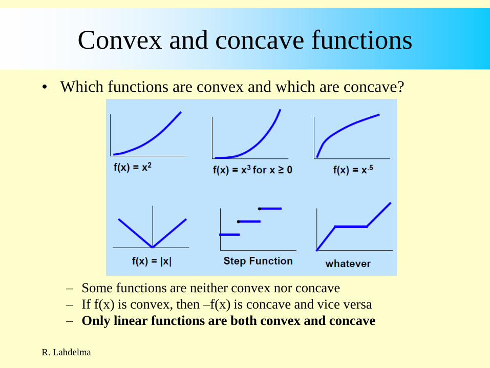
• Which functions are convex and which are concave?
– Some functions are neither convex nor concave
– If f(x) is convex, then –f(x) is concave and vice versa
– Only linear functions are both convex and concave
R. Lahdelma
Convex set
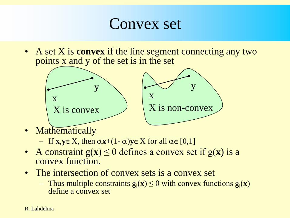
• A set X is convex if the line segment connecting any two points x and y of the set is in the set
• Mathematically – If x,yX, then x+(1- )yX for all [0,1]
• A constraint g(x) ≤ 0 defines a convex set if g(x) is a convex function.
• The intersection of convex sets is a convex set – Thus multiple constraints gi(x) ≤ 0 with convex functions gi(x)
define a convex set
x
y
X is convex
x y
X is non-convex

R. Lahdelma
Convex optimization problems
• Convex optimization problems are relatively easy to solve because
– A local optimum is also a global optimum
– They can be solved using hill-climbing strategy: starting from any feasible point move in a direction where f(x) improves while maintaining feasibility
– If the functions f(), g(), h() are smooth (first derivatives are continuous), various gradient-based methods can be used to identify improving directions
• Non-convex problems are difficult, because a local optimum is not in the general case a global optimum
R. Lahdelma
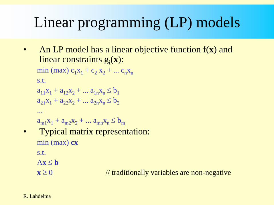
Linear programming (LP) models
• An LP model has a linear objective function f(x) and linear constraints gi(x):
min (max) c1x1 + c2 x2 + ... cnxn
s.t.
a11x1 + a12x2 + ... a1nxn b1
a21x1 + a22x2 + ... a2nxn b2
... am1x1 + am2x2 + ... amnxn bm
• Typical matrix representation:
min (max) cx
s.t.
Ax b
x 0 // traditionally variables are non-negative

R. Lahdelma
Linear programming (LP) models
• Special case of convex problems
– f(x), g(x) and h(x) are linear functions of x
– The constraints are (hyper-) planes in n dimensions
– The feasible area is an n-dimensional polyhedron
– The optimum is at a corner point at the intersection between some
constraint planes
• Very efficient solution algorithms for LP models exist
– The Simplex algorithm can solve LP models with millions of
variables and constraints
• Non-linear convex problems can be approximated by LP
models with arbitrarily good accuracy
• Non-convex problems cannot be represented as LP models

R. Lahdelma
How to define an LP model?
1. Write down a verbal explanation of what is the goal or
purpose of the model
– E.g. to minimize costs or maximize profit from some specific
operation or activity
2. Define the decision variables (and parameters)
– Use as descriptive or generic names as you like: x1, x2, fuel, …
– Give short description for them
– Also specify the unit (MWh, GJ, €/kg, m3/s, …)
3. Define the objective function to minimize or maximize
as a linear function of the variables
4. Define the constraints as linear inequality or equality
constraints for the variables

R. Lahdelma
LP example: Dual fuel condensing power plant
• Boiler can use two different fuels simultaneously in any proportion
• Boiler produces high pressure steam for a turbine driving a generator to produce electricity
• After turbine, steam is condensed back into water
• Fuels have different prices and consumption ratios
• Produced power is sold to market
• Typical objective is to maximize profit = revenue from selling power minus fuel costs
Power plant
- uses fuels
- produces power
Fuel 1
Fuel 2
Power

Dual fuel condensing power plant
26
h0 p
h
x1 h1
x2
High pressure steam header
Boiler
Feed water
Steam turbine G
Condenser

R. Lahdelma
LP example: Dual fuel condensing power plant
• Maximize profit during each hour of operation
• Decision variables
– x1, x2 fuel consumption (MWh)
– p power output (MWh)
• Parameters
– r1, r2 consumption ratios for fuels (1)
– c1, c2, c price for fuels and power (€/MWh)
– x1max, x2max upper bounds for fuel consumption (MWh)
– b hourly maximal production capacity (MWh)

R. Lahdelma
LP example: Dual fuel condensing power plant
• Objective function
max c*p - c1*x1 - c2*x2 // power sales minus fuel cost
• Constraints
p = x1/r1 + x2/r2 // power depends production
p b // capacity limit
x1 x1max,, x2 x2max, x1, x2 0
• Substitute expression for p to eliminate third variable
max (c/r1-c1)*x1 + (c/r2 - c2)*x2
x1/r1 + x2/r2 b // capacity limit
x1 x1max,, x2 x2max, x1, x2 0

R. Lahdelma
LP example:
Dual fuel condensing power plant, numerical
• Parameters
– Fuel consumption ratios (r1, r2) = (3.33, 2.5)
– Fuel & power prices (c1, c2, c) = (20, 25, 80) €/MWh
– Upper bounds for fuels (x1max, x2max) = (150,100) MWh
– Production capacity b = 60 MWh
max (80/3.33-20)*x1 + (80/2.5-25)*x2 = 4*x1 + 7*x2
0.3*x1 + 0.4*x2 60
x1 150
x2 100
x1, x2 0

R. Lahdelma
Graphical representation of LP models
• Models with two variables can be represented and solved graphically
– Linear constraints are drawn as lines
• The feasible region appears as a polygon
• The feasible region may be unbounded in some direction
• If the constraints are contradictory, the feasible region is empty and the model is infeasible
– Level curves of objective function f(x) = K = constant are draw as dotted lines
• Optimum is where a level curve touches the feasible region with with maximal or minimal K
• This happens at some corner
• If two corners yield optimal value, all points on the connecting edge are optimal (infinite number of optima)

R. Lahdelma
LP example:
Power plant model, graphical representation
max 4*x1 + 7*x2
0.3*x1 + 0.4*x2 60
x1 150
x2 100
x1, x2 0
Optimum at
x2=100
x1=66.7
0
50
100
150
200
0 50 100 150 200 250 300x1
x2
4x1+7x2=967
0.3x1+0.4x2=60
x1=150
x2=100
feasible region
optimum

R. Lahdelma
Properties of LP models
• Similar to a general optimization problem, an LP problem can be
– Feasible, if one or more feasible solutions exist
– Infeasible, if no feasible solutions exist, i.e. constraints are conflicting
• Example: min 0 s.t. x1, x0
– Unbounded, if infinitely good solutions exist
• Example: max x s.t. x0
• An LP problem has infinite number of optima if two or more corner solutions yield optimal value
– Then all convex combinations of optimal corner solutions are optimal

R. Lahdelma
LP example:
DH boiler
• A dual fuel boiler to produce district heat
– Goal to meet demand (MWh) as cheaply as possible
– Decision variables
• x1, x2 fuel consumption (MWh)
– Parameters
• r1, r2 consumption ratios for fuels (1)
• c1, c2 prices for fuels (€/MWh)
• x1max, x2max upper bounds for fuel consumption (MWh)
• b demand of heat
min c1*x1 + c2*x2
x1/r1 + x2/r2 b // allowed to produce excess
x1 x1max, x2 x2max, x1, x2 0
DH boiler
- uses fuels
- produces heat
Fuel 1
Fuel 2
Heat

R. Lahdelma
LP example:
DH boiler, numerical example
– Parameters
• Fuel consumption ratios (r1, r2) = (1.25, 1.11)
• Fuel prices (c1, c2) = (20, 25) €/MWh
• Upper bounds for fuels (x1max, x2max) = (150,100) MWh
• Heat demand b = 120
min 20*x1 + 25*x2;
0.8*x1 + 0.9*x2 120;
x1 150;
x2 100;
x1, x2 0;

R. Lahdelma
Solving LP problems – canonical form
• The simplex algorithm for LP problems is based
on solving linear equation systems
– First the problem is reformulated into canonical form,
where all constraints are of equality type
min (max) cx min (max) cx
s.t. s.t.
Ax b Ax + s = b
x 0 x,s 0
– s = [s1, s2, ..., sm]T is a vector of slack variables
– Greater than –type equations get surplus variables
Ax b Ax - s = b -Ax + s = -b

R. Lahdelma
Solving LP problems – canonical form
– In canonical form, the LP problem can be rewritten as
min (max) cx
s.t.
Ax = b
x 0
– The new A-matrix contains the original A and an
identity matrix A = [A|I]
– The new x-vector contains the original decision
variables and the slacks xT = [xT|sT]
– The new c-vector contains the original c and zeros as
cost coefficients for the slacks

R. Lahdelma
Solving LP problems – canonical form
• The original problem contained m constraints and n variables
– In canonical form the problem contains m constraints and m+n variables
• n original decision variables and m slacks
• The A-matrix is more wide than tall
– Thus, there are more variables than equations
• Such an underdetermined system has in general an infinite number of solutions
– The idea is to fix n of the variables to zero (their lower bounds) and solve the remaining m variables from the m equations

R. Lahdelma
Solving LP problems – basic solutions
• The Simplex algorithm explores basic solutions of the equation system – A basis is a set of m linearly independent columns of
the A-matrix
– We partition A = [B|N] where B is the basis and N is the non-basic part
– x is partitioned similarly into basic variables xB and non-basic xN
– c is partitioned similarly into cB and cN
• The problem is rewritten as min (max) cBxB + cNxN
s.t.
BxB + NxN = b
xB, xN 0

R. Lahdelma
Solving LP problems – basic solutions
min (max) cBxB + cNxN
s.t.
BxB + NxN = b
xB, xN 0
– A basic solution is obtained by setting xN = 0 and solving
xB = B-1(b- NxN) = B-1b
• Basic solutions correspond to corner points, i.e. intersections between constraint equations – When a slack is non-basic (zero) the constraint is
active (equality holds)
– When a slack is non-zero, the constraint is inactive (strict inequality)
– A basic solution is feasible if (and only if) xB 0

R. Lahdelma
Solving LP problems – basic solution example
• The power plant problem in canonical form
A = [0.3 0.4 1 0 0;
1 0 0 1 0;
0 1 0 0 1]
– Select x1,x2, s2 as basic and s1=s3=0 non-basic
0.3*x1 + 0.4*x2 = 60
x1 + s2 = 150
x2 = 100
x2 = 100; x1 = (60-40)/0.3 = 67; s2 = 150-67 = 83
Objective = 4*67 + 7*100 = 967 (this happens to be optimum, see graph)
max 4*x1 + 7*x2;
0.3*x1 + 0.4*x2 60
x1 150
x2 100
x1, x2 0
max 4*x1 + 7*x2;
0.3*x1 + 0.4*x2 + s1 = 60
x1 + s2 = 150
x2 +s3 = 100
x1, x2, s1, s2, s3 0

R. Lahdelma
Solving LP problems – basic solutions
• In principle LP problems could be solved by
– computing all basic solutions and
– selecting among the feasible ones the one with optimal
objective function value
– But the number of basic solutions is potentially
• m = number of constrains, n = number of decision variables
– Already with m=n=20 there are 137 846 528 820
combinations
!!
)!(
nm
nm
m
nm

R. Lahdelma
Solving LP problems – Simplex algorithm
• The Simplex algorithm searches the optimum among the basic solutions
– It starts with some basic solutions such as slack-basis
– It moves to an adjacent basic solution so that the solution improves
• In an adjacent basic solution exactly one variable is replaced in the basis
• graphically it means moving between corners along an edge
– This is repeated until optimum is found
• Theoretically the Simplex algorithm may explore an exponential number of basic solutions
– In practice the algorithm is fast and polynomial in complexity

CHP – Combined Heat and Power
43
• Cogeneration means production of two or more
energy products together in an integrated process – CHP = combined heat and power generation
– Trigeneration: • district heating + cooling + power
• high pressure process heat + low pressure heat + power
– Technologies: backpressure turbines, combined
steam&gas turbines, combustion engine with excess
heat utilization …
– Much more efficient than producing the products
separately – over 90% efficiency possible
– Cost-efficient way to reduce CO2 emissions

CHP planning
44
• Objective is to maximize profit s.t. production constraints
• Hourly production of the different products must be
planned together – Production of heat & cooling must meet the demand (natural
monopoly)
– Power production is planned to maximize the profit from sales to
the spot market (free market)
• A long-term model consists of many hourly models in
sequence – E.g. an annual model consists of 8760 hourly models
– Hourly forecasts for demand and power price
• Various advanced analyses, e.g. risk analysis require
solving many long-term models – Solution must be fast!

Sample backpressure/bleeder turbine plant
45
h0
p
h v01
h1
h2
f1 h3 r = v01+h1-v12
f2
v12
q = v12+h2
High pressure steam header
Boiler
Feed water
Steam
turbine
Medium pressure steam
Low pressure steam
G
Condenser
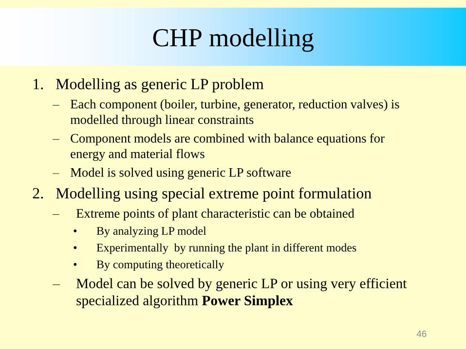
CHP modelling
46
1. Modelling as generic LP problem
– Each component (boiler, turbine, generator, reduction valves) is
modelled through linear constraints
– Component models are combined with balance equations for
energy and material flows
– Model is solved using generic LP software
2. Modelling using special extreme point formulation
– Extreme points of plant characteristic can be obtained
• By analyzing LP model
• Experimentally by running the plant in different modes
• By computing theoretically
– Model can be solved by generic LP or using very efficient
specialized algorithm Power Simplex

R. Lahdelma
LP modelling technique using convex
combination
• Weighted average = linear interpolation between two points
– P = xP1 + (1-x)P2 with x[0,1] is a convex combination of coordinates P1 and P2.
P1
P2
P=0.6P1+0.4P2

R. Lahdelma
LP modelling technique using convex
combination
• Equivalent formulation with two weights x1& x2
P = x1P1 + x2P2 where x1+x2 = 1, x1,x20.
• More generally for any number of points Pj
P = j xjPj where j xj = 1, xj0.
• Expressions are linear with respect to xj
– Points can be scalars (1-dimensional case) or
– Points can be vectors (multiple dimensions)
P1
P2
P=0.6P1+0.4P2

LP model for CHP plant – LP-encoding of
convex characteristic operating region
49
• The power plant characteristic defines the feasible
operating area in the 3D space (c,p,q)
– p = power production, q = heat production, c = cost
• Encode model as a convex combination of extreme
(corner) points
max cpp – C // cp is power price
s.t.
j cjxj = C // variable prod. cost
j pjxj = P // variable power prod.
j qjxj = Q // fixed heat demand
j xj = 1 // convex comb.
xj 0
Q (c3,p3,q3)
(c4,p4,q4)
(c2,p2,q2)
(c5,p5,q5)
(c6,p6,q6)
(c1,p1,q1) P

LP model for CHP plant – LP-encoding of
convex characteristic operating region
Jjx
Qxq
Pxp
x
xc
j
Jj
jj
Jj
jj
Jj
j
Jj
jj
u
u
u
,0
1
min
3.12.20117 R.Lahdelma 50

Hourly trigeneration model
51
• Extreme point formlation with three commodities
(p,q,r), multiple plants and multiple periods
– Extreme points are in 4D space
– Index t for hour, index u for plant in set of plants U
– Ju = set of extreme points of plant u
),,,( tj
tj
tj
tj rqpc
uJj
tj
tj
tu xcC
uJj
tj
tj
tu xpP
uJj
tj
tj
tu xqQ
uJj
tj
tj
tu xrR
1 uJj
tjx
0tjx uU

R. Lahdelma
Review questions
• Please review lecture material and be prepared to answer review questions at next lecture
1. Is the optimization problem max x2 + y2 s.t. x,y0 feasible, infeasible or unbounded? Why?
2. Give a feasible solution to the above problem.
3. How many optimal solutions does the problem max x2 s.t. -5x5 have?
4. Transform max x s.t. x5 replacing inequality constraint by equality constraint.
5. Transform max x s.t. x5 into an unconstrained optimization problem.
6. Why is classification of optimization problems important?
7. Classify the following optimization problem: min x2 + y2 s.t. x,y0, xR, yN
8. Why is LP modelling so common?
9. Why are convex optimization problems relatively easy to solve?
10. Give an example of an optimization problem which is difficult or impossible to solve.
11. Does LP apply to non-linear problems? Why, or why not?
12. When can an LP problem have infinite number of optimal solutions?
13. Give an example of an infeasible LP problem
14. Give an examle of a feasible LP problem without optimal solution
15. Give an example of an LP problem with infinite number of optima