linear operators and adjoints - university of michiganfessler/course/600/l/l06.pdf · 6.2 c j....

Chapter 6

Linear operators and adjoints

Contents

Introduction . . . . . . . . . . . . . . . . . . . . . . . . . . . . . . . . . . . . . . . . . .. . . . . . . . . . . . . 6.1

Fundamentals . . . . . . . . . . . . . . . . . . . . . . . . . . . . . . . . . . . . . . . . .. . . . . . . . . . . . . 6.2

Spaces of bounded linear operators . . . . . . . . . . . . . . . . . . . . . . . .. . . . . . . . . . . . . . . . . . . 6.3

Inverse operators . . . . . . . . . . . . . . . . . . . . . . . . . . . . . . . . . . . .. . . . . . . . . . . . . . . . . 6.5

Linearity of inverses . . . . . . . . . . . . . . . . . . . . . . . . . . . . . . . . . . . .. . . . . . . . . . . . . . . 6.5

Banach inverse theorem . . . . . . . . . . . . . . . . . . . . . . . . . . . . . . . . .. . . . . . . . . . . . . . . . 6.5

Equivalence of spaces . . . . . . . . . . . . . . . . . . . . . . . . . . . . . . . . .. . . . . . . . . . . . . . . . . 6.5

Isomorphic spaces . . . . . . . . . . . . . . . . . . . . . . . . . . . . . . . . . . . .. . . . . . . . . . . . . . . . 6.6

Isometric spaces . . . . . . . . . . . . . . . . . . . . . . . . . . . . . . . . . . . . . .. . . . . . . . . . . . . . . 6.6

Unitary equivalence . . . . . . . . . . . . . . . . . . . . . . . . . . . . . . . . . . . .. . . . . . . . . . . . . . . 6.7

Adjoints in Hilbert spaces . . . . . . . . . . . . . . . . . . . . . . . . . . . . . . . . . .. . . . . . . . . . . . . . 6.11

Unitary operators . . . . . . . . . . . . . . . . . . . . . . . . . . . . . . . . . . . . . .. . . . . . . . . . . . . . 6.13

Relations between the four spaces . . . . . . . . . . . . . . . . . . . . . . . . . . .. . . . . . . . . . . . . . . . . 6.14

Duality relations for convex cones . . . . . . . . . . . . . . . . . . . . . . . . . . .. . . . . . . . . . . . . . . . . 6.15

Geometric interpretation of adjoints . . . . . . . . . . . . . . . . . . . . . . . . . . . .. . . . . . . . . . . . . . . 6.15

Optimization in Hilbert spaces . . . . . . . . . . . . . . . . . . . . . . . . . . . . . . . .. . . . . . . . . . . . . . 6.16

The normal equations . . . . . . . . . . . . . . . . . . . . . . . . . . . . . . . . . . .. . . . . . . . . . . . . . . 6.16

The dual problem . . . . . . . . . . . . . . . . . . . . . . . . . . . . . . . . . . . . . .. . . . . . . . . . . . . . 6.17

Pseudo-inverse operators . . . . . . . . . . . . . . . . . . . . . . . . . . . . . .. . . . . . . . . . . . . . . . . . 6.18

Analysis of the DTFT . . . . . . . . . . . . . . . . . . . . . . . . . . . . . . . . . . . . .. . . . . . . . . . . . . 6.21

6.1Introduction

The field of optimization uses linear operators and their adjoints extensively.

Example. differentiation,convolution, Fourier transform , Radon transform, among others.

Example. If A is a n × m matrix, an example of a linear operator, then we know that‖y − Ax‖2 is minimized whenx =

[A′A]−1A′y.

We want to solve such problems for linear operators between more general spaces. To do so, we need to generalize “transpose”and “inverse.”

6.1

6.2 c© J. Fessler, December 21, 2004, 13:3 (student version)

6.2Fundamentals

We writeT : D → Y whenT is a transformation from a setD in a vector spaceX to a vector spaceY.

The setD is called thedomain of T . Therangeof T is denoted

R(T ) = {y ∈ Y : y = T (x) for x ∈ D} .

If S ⊆ D, then theimageof S is given by

T (S) = {y ∈ Y : y = T (s) for s ∈ S} .

If P ⊆ Y, then theinverse imageof P is given by

T−1(P ) = {x ∈ D : T (x) ∈ P} .

Notation: for alinear operator A, we often writeAx instead ofA(x).

For linear operators, we can always just useD = X , so we largely ignoreD hereafter.

Definition. Thenullspaceof a linear operatorA is N(A) = {x ∈ X : Ax = 0} .It is also called thekernel of A, and denotedker(A).

Exercise. For a linear operatorA, the nullspaceN(A) is asubspaceof X .Furthermore, ifA is continuous (in a normed spaceX ), thenN(A) is closed[3, p. 241].

Exercise. The range of a linear operator is asubspaceof Y.

Proposition. A linear operator on a normed spaceX (to a normed spaceY) is continuous at every pointX if it is continuousat a single point inX .

Proof.Exercise. [3, p. 240].

Luenberger does not mention thatY needs to be a normed space too.

Definition. A transformationT from a normed spaceX to a normed spaceY is calledboundediff there is a constantM such that‖T (x)‖ ≤ M ‖x‖ , ∀x ∈ X .

Definition. The smallest suchM is called thenorm of T and is denoted|||T |||. Formally:

|||T ||| , inf {M ∈ R : ‖T (x)‖ ≤ M ‖x‖ , ∀x ∈ X} .

Consequently:‖T (x)‖Y ≤ |||T ||| ‖x‖X , ∀x ∈ X .

Fact. For alinear operatorA, an equivalent expression (used widely!) for the operator norm is

|||A||| = sup‖x‖≤1

‖Ax‖ .

Fact. If X is the trivial vector space consisting only of the vector0, then|||A||| = 0 for any linear operatorA.

Fact. If X is a nontrivial vector space, then for alinear operatorA we have the following equivalent expressions:

|||A||| = supx6=0

‖Ax‖‖x‖ = sup

‖x‖=1

‖Ax‖ .

c© J. Fessler, December 21, 2004, 13:3 (student version) 6.3

. . . . . . . . . . . . . . . . . . . . . . . . . . . . . . . . . . . . . . . . . . . . . . . . . . .. . . . . . . . . . . . . . . . . . . . . . . . . . . . . . . . . . . . . . . . . . . . . . . . . . .. . . . . . . . . . . . . . . .Example. ConsiderX = (Rn, ‖·‖∞) andY = R.

ClearlyAx = a1x1+· · ·+anxn so‖Ax‖Y = |Ax| = |a1x1+· · ·+anxn| ≤ |a1||x1|+· · ·+|an||xn| ≤ (|a1|+· · ·+|an|) ‖x‖∞ .In fact, if we choosex such thatxi = sgn(ai), then‖x‖∞ = 1 we get equality above. So we conclude|||A||| = |a1| + · · · + |an|.

Example. What if X =(

Rn, ‖·‖p

)

? ??

Proposition. A linear operator is bounded iff it is continuous.

Proof.Exercise. [3, p. 240].

More facts related to linear operators.• If A : X → Y is linear andX is a finite-dimensional normed space, thenA is continuous [3, p. 268].• If A : X → Y is a transformation whereX andY are normed spaces, thenA is linear andcontinuous iff A(

∑∞i=1 αixi) =

∑∞i=1 αiA(xi) for all convergent series

∑∞i=1 αixi. [3, p. 237].

This is thesuperposition principle as described in introductory signals and systems courses.

Spaces of bounded linear operators

Definition. If T1 andT2 are both transformations with a common domainX and a common rangeY, over a common scalar field,then we define natural addition and scalar multiplication operations as follows:

(T1 +T2)(x) = T1(x) +T2(x)

(α T1)(x) = α(T1(x)).

Lemma. With the preceding definitions, whenX andY are normed spaces the following space ofoperators(!) is avector space:

B(X ,Y) = {bounded linear transformations fromX toY} .

(The proof that this is a vector space is within the next proposition.)

This space is analogous to certain types ofdual spaces (seeCh. 5).

Not only isB(X ,Y) a vector space, it is a normed space when one uses the operatornorm |||A||| defined above.

Proposition. (B(X ,Y), ||| · |||) is a normed space whenX andY are normed spaces.

Proof. (sketch)

Claim 1.B(X ,Y) is a vector space.SupposeT1, T2 ∈ B(X ,Y) andα ∈ F .

‖(α T1 +T2)(x)‖Y = ‖α T1(x)+T2(x)‖Y ≤ |α| ‖T1(x)‖Y + ‖T2(x)‖Y ≤ |α||||T1 ||| ‖x‖X + |||T2 ||| ‖x‖X = K ‖x‖X , whereK , |α||||T1 ||| + |||T2 |||. Soα T1 +T2 is a bounded operator. Clearlyα T1 +T2 is a linear operator.

Claim 2. ||| · ||| is a norm onB.The “hardest” part is verifying the triangle inequality:

|||T1 +T2 ||| = sup‖x‖=1

‖(T1 +T2)x‖Y ≤ sup‖x‖=1

‖T1 x‖Y + sup‖x‖=1

‖T2 x‖Y = |||T1 ||| + |||T2 |||.

2

Are there other valid norms for B(X ,Y)? ??

Remark.We did not really “need” linearity in this proposition. We could have shown that the space of bounded transformationsfromX toY with ||| · ||| is a normed space.


Not only isB(X ,Y) a normed space, but it is evencompleteif Y is.

Theorem. If X andY are normed spaces withY complete, then(B(X ,Y), ||| · |||) is complete.

Proof.

Suppose{Tn} is a Cauchy sequence (inB(X ,Y)) of bounded linear operators,i.e., |||Tn − Tm||| → 0 asn,m → ∞.

Claim 0.∀x ∈ X , the sequence{Tn(x)} is Cauchy inY.

‖Tn(x) − Tm(x)‖Y = ‖(Tn − Tm)(x)‖Y ≤ |||Tn − Tm||| ‖x‖X → 0 asn,m → ∞.

SinceY is complete, for anyx ∈ X the sequence{Tn(x)} converges to some point inY. (This is calledpointwise convergence.)So we can define an operatorT : X → Y by T (x) , limn→∞ Tn(x).

To showB is complete, we must first showT ∈ B, i.e., 1) T is linear, 2)T is bounded.Then we show 3)Tn → T (convergence w.r.t. the norm||| · |||).Claim 1.T is linear

T (αx + z) = limn→∞

Tn(αx + z) = limn→∞

[αTn(x) + Tn(z)] = α T (x)+T (z) .

(Recall that in a normed space, ifun → u andvn → v, thenαun + vn → αu + v.)

Claim 2:T is boundedSince{Tn} is Cauchy, it is bounded, so∃K < ∞ s.t. |||Tn||| ≤ K, ∀n ∈ N. Thus, by the continuity of norms, for anyx ∈ X :

‖T (x)‖Y = limn→∞

‖Tn(x)‖Y ≤ limn→∞

|||Tn||| ‖x‖X ≤ K ‖x‖X .

Claim 3:Tn → TSince{Tn} is Cauchy,

∀ε > 0, ∃N ∈ N s.t.n,m > N =⇒ |||Tn − Tm||| ≤ ε

=⇒ ‖Tn(x) − Tm(x)‖Y ≤ ε ‖x‖X , ∀x ∈ X=⇒ lim

m→∞‖Tn(x) − Tm(x)‖Y ≤ ε ‖x‖X , ∀x ∈ X

=⇒ ‖Tn(x) − T (x)‖Y ≤ ε ‖x‖X , ∀x ∈ X by continuity of the norm

=⇒ |||Tn − T ||| ≤ ε.

We have shown that every Cauchy sequence inB(X ,Y) converges to some limit inB(X ,Y), soB(X ,Y) is complete. 2

Corollary . (B(X , R), ||| · |||) is a Banach space for any normed spaceX .

Why? ??

We writeA ∈ B(X ,Y) as shorthand for “A is a bounded linear operator from normed spaceX to normed spaceY.”. . . . . . . . . . . . . . . . . . . . . . . . . . . . . . . . . . . . . . . . . . . . . . . . . . .. . . . . . . . . . . . . . . . . . . . . . . . . . . . . . . . . . . . . . . . . . . . . . . . . . .. . . . . . . . . . . . . . . .Definition. In general, ifS : X → Y and T : Y → Z, then we can define theproduct operator or composition as atransformationT S : X → Z by (T S)(x) = T (S(x)).

Proposition. If S ∈ B(X ,Y) andT ∈ B(Y,Z), thenT S ∈ B(X ,Z).

Proof.Linearity of the composition of linear operators is trivialto show.To show that the composition is bounded:‖T Sx‖Z ≤ |||T ||| ‖Sx‖Y ≤ |||T ||||||S||| ‖x‖X . 2

Does it follow that |||T S||| = |||T ||||||S|||? ??


6.3Inverse operators

Definition. T : X → Y is calledone-to-onemapping ofX intoY iff x1,x2 ∈ X andx1 6= x2 =⇒ T (x1) 6= T (x2).

Equivalently,T is one-to-oneif the inverse image of any pointy ∈ Y is at most a single point inX , i.e.,∣∣T−1({y})

∣∣ ≤ 1, ∀y ∈ Y.

Definition. T : X → Y is calledonto iff T (X ) = Y. This is a stronger condition thaninto.

Fact. If T : X → Y is one-to-oneandontoY, thenT has aninversedenotedT−1 such thatT (x) = y iff T−1(y) = x.

Many optimization methods,e.g., Newton’s method, require inversion of theHessianmatrix (or operator) corresponding to a costfunction.

Lemma. [3, p. 171]If A : X → Y is a linear operator between two vector spacesX andY, thenA is one-to-oneiff N(A) = {0}.

Linearity of inverses

We first look at the algebraic aspects of inverse operators invector spaces.

Proposition. If a linear operatorA : X → Y (for vector spacesX andY) has an inverse, then that inverseA−1 is also linear.

Proof.SupposeA−1(y1) = x1, A−1(y2) = x2, A(x1) = y1, andA(x2) = y2. Then by the linearity ofA we haveA(αx1+x2) =αAx1 + Ax2 = αy1 + y2, soA−1(αy1 + y2) = αx1 + x2 = αA−1(y1) + A−1(y2). 2

6.4Banach inverse theorem

Now we turn to the topological aspects, in normed spaces.

Lemma. (Baire) A Banach spaceX is not the union of countably many nowhere dense sets inX .Proof.see text

Theorem. (Banach inverse theorem)If A is a continuous linear operator from a Banach spaceX onto a Banach spaceY for which the inverse operatorA−1 exists,thenA−1 is continuous.

Proof.see text

Combining with the earlier Proposition that linear operators are bounded iff they are continuous yields the following.

Corollary .X ,Y Banach andA ∈ B(X ,Y) andA invertible=⇒ A−1 ∈ B(Y,X )

Equivalence of spaces(one way to use operators)• in vector spaces• in normed spaces• in inner product spaces

spaces relation operator requirementsvector isomorphic isomorphism linear, onto, 1-1normed topologically isomorphic topological isomorphism linear, onto, invertible, continuousnormed isometrically isomorphic isometric isomorphism linear, onto, norm preserving=⇒ 1-1, continuousinner product unitarily equivalent unitary isometric isomorphism that preserves inner products


Isomorphic spaces

Definition. Vector spacesX andY are calledisomorphic (think: “same structure”) iff there exists aone-to-one, linear mappingT of X ontoY.In such cases the mappingT is called anisomorphism of X ontoY.Since anisomorphismT is one-to-oneandonto, T is invertible , and by the “linear of inverses” proposition in6.3, T−1 is linear.

Example. ConsiderX = R2 andY = {f(t) = a + bt on [0, 1] : a, b ∈ R}.

An isomorphism isf = T (x) ⇐⇒ f(t) = a + bt wherex = (a, b), with inverseT−1(f) = (f(0), f(1) − f(0)).

Exercise. Any realn-dimensional vector space is isomorphic toRn (problem 2.14 p. 44) [3, p. 268].

However, they need not be topologically isomorphic [3, p. 270].. . . . . . . . . . . . . . . . . . . . . . . . . . . . . . . . . . . . . . . . . . . . . . . . . . .. . . . . . . . . . . . . . . . . . . . . . . . . . . . . . . . . . . . . . . . . . . . . . . . . . .. . . . . . . . . . . . . . . .So far we have said nothing about norms. In normed spaces we can have a topological relationship too.

Definition. Normed spacesX andY are calledtopologically isomorphic iff there exists acontinuous linear transformationT ofX ontoY having a continuous inverseT−1. The mappingT is called atopological isomorphism.

Theorem. [3, p. 258] Two normed spaces aretopologically isomorphic iff there exists a linear transformationT with domainX and rangeY and positive constantsm andM s.t.m ‖x‖X ≤ ‖T x‖Y ≤ M ‖x‖X , ∀x ∈ X .

Example. In the previous example, consider(X , ‖·‖∞) and(Y, ‖·‖2). Then for the sameT described in that example:

x = (a, b) =⇒ ‖T (x)‖2Y =

∫ 1

0(a + bt)2 dt = a2 + ab + b2/3 ≤ a2 + |a| |b| + b2/3 ≤ (1 + 1 + 1/3) ‖x‖2

∞ = 7/3 ‖x‖2∞ .

Also ‖T (x)‖2Y = a2 + ab + b2/3 = (a + b/2)2 + b2/12 = (a

√3/2 + b/

√3)2 + a2/4 ≥ ‖x‖2

∞ /12.SoX andY are topologically isomorphic for the given norms.

Exercise. (C[0, 1], ‖·‖∞) and(C[0, 1], ‖·‖1) are not topologically isomorphic.Why? ??

Isometric spaces

Definition. LetX andY be normed spaces. A mappingT : X → Y is callednorm preserving iff ‖T (x)‖Y = ‖x‖X , ∀x ∈ X .

In particular, ifT is norm preserving, then|||T ||| = 1. What about the converse? ??

Proposition. If T is linear and norm preserving, thenT is one-to-one, i.e., T (x) = T (z) =⇒ x = z.

Proof. If T (x) = y andT (z) = y, then by linearityT (x − z) = 0.So sinceT is norm preserving,‖x − z‖ = ‖0‖ = 0, sox = z. 2

. . . . . . . . . . . . . . . . . . . . . . . . . . . . . . . . . . . . . . . . . . . . . . . . . . .. . . . . . . . . . . . . . . . . . . . . . . . . . . . . . . . . . . . . . . . . . . . . . . . . . .. . . . . . . . . . . . . . . .Definition. If T : X → Y is both linear and norm preserving, thenT is called alinear isometry.

If, in addition,T is ontoY, thenX andY are calledisometrically isomorphic, andT is called anisometric isomorphism.

Remark.To illustrate why we requireonto here, considerT : En → `2 defined byT (x) = (x1, . . . , xn, 0, 0, . . .).

ThisT is linear, one-to-one, and norm preserving, but not onto.

Exercise. Every normed spaceX is isometrically isomorphic to a dense subset of a Banach spaceX .(problem 2.15 on p. 44)

Normed spaces that are isometrically isomorphic can, in some sense, be treated as being identical,i.e., they have identical proper-ties. However, the specific isomorphism can be important sometimes.

Example. ConsiderY = `p(N) = {(a1, a2, . . .) :∑∞

i=1 |ai|p < ∞}andX = `p(Z) =

{(. . . , a−2, a−1, a0, a1, a2, . . .) :

∑∞i=−∞ |ai|p < ∞

}. Define the mappingT : X → Y byy = (b1, b2, . . .) =

T (x) if bi = az(i) wherez(i) = (−1)i bi/2c . Note thatz : {1, 2, 3, . . .} → 0, 1,−1, 2,−2, . . ..

This mappingT is clearly an isometric isomorphism, so “`p (Z)” and “`p (N)” are isometrically isomorphic. Hence we only botherto work with `p = `p(N) since we know all algebraic and topological results will carry over to double-sided sequences.


Unitary equivalence in inner product spaces

Definition. Two inner product spacesX andY areunitarily equivalent iff there is anisomorphism U : X → Y of X onto Ythat preserves inner products:〈Ux1, Ux2〉Y = 〈x1, x2〉X , ∀x1,x2 ∈ X . The mappingU is called aunitary operator .

Fact. If U is unitary, thenU is norm preserving since‖Ux‖ = 〈Ux, Ux〉 = 〈x, x〉 = ‖x‖ . Clearly|||U ||| = 1.Furthermore, sinceU is onto,U is anisometric isomorphism. Interestingly, the converse is also true [3, p. 332].

Theorem. A mappingU of X onto Y, whereX andY are inner product spaces, is an isometric isomorphism iffU is aunitary operator.

Proof. (⇐=) was just argued above.(=⇒) SupposeU is an isometric isomorphism.Using the parallelogram law, the linearity ofU , and the fact that‖Ux‖ = ‖x‖, we have:

4 〈Ux, Uy〉 = ‖Ux + Uy‖2 − ‖Ux − Uy‖2+ i ‖Ux + iUy‖2 − i ‖Ux − iUy‖2

= ‖U(x + y)‖2 − ‖U(x − y)‖2+ i ‖U(x + iy)‖2 − i ‖U(x − iy)‖2

= ‖x + y‖2 − ‖x − y‖2+ i ‖x + iy‖2 − i ‖x − iy‖2

= 4 〈x, y〉 .

ThusU an isometric isomorphism=⇒ U unitary. 2

Remark.After defining adjoints we will show thatU−1 = U? in Hilbert spaces.

Exercise. Any complexn-dimensional inner product space is unitarily equivalent to Cn [3, p. 332].

Every separable Hilbert space is unitarily equivalent with`2 or someCn [3, p. 339].

Example. Continue the previousf(t) = a + bt example, but now useEn and(Y, 〈·, ·〉2). If g(t) = c + dt then

〈T x1, T x2〉 = 〈f, g〉 =

∫ 1

0

f(t)g(t) dt =

∫ 1

0

(a+bt)(c+dt) dt = ac+ad

2+

bc

2+

bd

3= [a b]

[1 1/2

1/2 1/3

] [cd

]

= x′1Gx2,

so we defineU = T G−1/2, then

〈Ux1, Ux2〉 = 〈T G−1/2x1, T G−1/2x2〉 = (G−1/2x1)′G(G−1/2x1) = x′

1x1 = 〈x1, x2〉 .

Example. The Fourier transformF (ν) =∫∞−∞ f(t) e−ı2πνt dt is a unitary mapping ofL2[R] onto itself.

Example. Soon we will analyze thediscrete-time Fourier transform (DTFT ) operator, defined by

G = Fg ⇐⇒ G(ω) =

∞∑

n=−∞gn eıωn .

We will show thatF ∈ B(`2,L2[−π, π]) andF is invertible. And Parseval’s relation from Fourier analysis is that

⟨1√2π

Fg,1√2π

Fh

⟩

=1

2π

∫ π

−π

G(ω)H∗(ω) dω =∞∑

n=−∞gnh∗

n = 〈g, h〉 .

So`2 andL2[−π, π] are unitarily equivalent, and the unitary operator needed is simplyU = 1√2π

F .


The following “extension theorem” is useful in proving thatevery separable Hilbert space is isometrically isomorphicto `2.

Theorem. Let X be a normed space,Y a Banach space, andM ⊂ X and N ⊂ Y be subspaces.Suppose that• M = X , andN = Y,• T : M → N is a bounded linear operator.

Then there exists a unique linear operatorT : X → Y such thatT |M = T . Moreover,|||T ||| = ||| T |||.If, in addition,• X is a Banach space,• T

−1

: N → M exists and is bounded,thenT is alsoonto Y.

Proof.Note:T |M readsT restricted toM .

T |M = T meansT (x) = T (x) for all x ∈ M .. . . . . . . . . . . . . . . . . . . . . . . . . . . . . . . . . . . . . . . . . . . . . . . . . . .. . . . . . . . . . . . . . . . . . . . . . . . . . . . . . . . . . . . . . . . . . . . . . . . . . .. . . . . . . . . . . . . . . .Claim 1. If {xn} ∈ M is Cauchy inM , then

{

T (xn)}

is Cauchy inN .∥∥∥T (xn)− T (xm)

∥∥∥Y

=∥∥∥T (xn − xm)

∥∥∥Y≤ ||| T ||| ‖xn − xm‖X → 0 asn,m → ∞.

. . . . . . . . . . . . . . . . . . . . . . . . . . . . . . . . . . . . . . . . . . . . . . . . . . .. . . . . . . . . . . . . . . . . . . . . . . . . . . . . . . . . . . . . . . . . . . . . . . . . . .. . . . . . . . . . . . . . . .Claim 2. For{xn} , {xn} ∈ M , supposexn → x ∈ X andxn → x.

Then{

T (xn)}

and{

T (xn)}

both converge and to the same limit.{

T (xn)}

and{

T (xn)}

are both Cauchy inN by Claim 1 sincexn andxn both converge.

SinceY is complete,∃y, y ∈ Y s.t. T (xn) → y and T (xn) → y.

But ‖y − y‖Y = limn→∞∥∥∥T (xn)− T (xn)

∥∥∥Y

= limn→∞∥∥∥T (xn − xn)

∥∥∥Y≤ limn→∞ ||| T ||| ‖xn − xn‖X

= ||| T ||| ‖x − x‖X = 0, using norm continuity, linearity ofT , and boundedness ofT .

Now we defineT : X → Y as follows.Forx ∈ X = M , ∃ {xn} ∈ M such thatxn → x, so we defineT (x) , limn→∞ T (xn).By Claim 2,T is well-defined, and moreover, ifx ∈ M , thenT (x) = T (x), i.e., T |M = T .. . . . . . . . . . . . . . . . . . . . . . . . . . . . . . . . . . . . . . . . . . . . . . . . . . .. . . . . . . . . . . . . . . . . . . . . . . . . . . . . . . . . . . . . . . . . . . . . . . . . . .. . . . . . . . . . . . . . . .Claim 3. |||T ||| = ||| T |||∀x ∈ X , T (x) = limn→∞ T (xn) wherexn ∈ M andxn → x.

Thus‖T (x)‖Y = limn→∞∥∥∥T (xn)

∥∥∥Y≤ limn→∞ ||| T ||| ‖xn‖X = ||| T ||| ‖x‖X . Thus|||T ||| ≤ ||| T |||.

However,∀x ∈ M , T (x) = T (x) =⇒ |||T ||| ≥ ||| T |||, sinceT is defined onX ⊇ M .Thus|||T ||| = ||| T |||.. . . . . . . . . . . . . . . . . . . . . . . . . . . . . . . . . . . . . . . . . . . . . . . . . . .. . . . . . . . . . . . . . . . . . . . . . . . . . . . . . . . . . . . . . . . . . . . . . . . . . .. . . . . . . . . . . . . . . .Claim 4.T is linear, which is trivial to prove.. . . . . . . . . . . . . . . . . . . . . . . . . . . . . . . . . . . . . . . . . . . . . . . . . . .. . . . . . . . . . . . . . . . . . . . . . . . . . . . . . . . . . . . . . . . . . . . . . . . . . .. . . . . . . . . . . . . . . .Claim 5. (uniqueness ofT ) If L1, L2 ∈ B(X ,Y), thenL1|M = L2|M =⇒ L1 = L2.Forx ∈ X = M , ∃ {xn} ∈ M s.t.xn → x. Thus, by the continuity ofL1 andL2,L1(x) = limn→∞ L1(xn) = limn→∞ L2(xn) = L2(x), sinceL1(xn) = L2(xn) by L1|M = L2|M .

. . . . . . . . . . . . . . . . . . . . . . . . . . . . . . . . . . . . . . . . . . . . . . . . . . .. . . . . . . . . . . . . . . . . . . . . . . . . . . . . . . . . . . . . . . . . . . . . . . . . . .. . . . . . . . . . . . . . . .Claim 6. If T

−1: N → M exists and is bounded, and ifX is a Banach space, thenT is ontoY.

Let y ∈ Y. SinceN = Y, ∃ {yn} ∈ N s.t.yn → y.

By the same reasoning as in Claim 1,xn = T−1

(yn) is Cauchy inX .

SinceX is a Banach space,∃x ∈ X s.t.xn → x.

ThusT (x) = limn→∞ T (xn) = limn→∞ T(

T−1

(yn

)

) = limn→∞ yn = y.

Thus,∀y ∈ Y, ∃x ∈ X s.t.T (x) = y. 2


The following theorem is an important application of the previous theorem.

Theorem. Every separable Hilbert spaceH is isometrically isomorphic to2.

Proof.

H separable=⇒ ∃ a countable orthonormal basis{ei}. (Homework.) LetM = [{ei}∞i=1].

Of course 2 has a countable orthonormal basis{ei}, whereeij = δi−j (Kronecker). LetN = [{ei}∞i=1].

DefineT : M → N to be the linear operator for whichT (ei) = ei.(Exercise.Think about why “the” here—considerM .)

Then since anyx ∈ M has formx =∑n

i=1ciei for somen ∈ N:

∥∥∥T (x)

∥∥∥

2

=

∥∥∥∥∥T

(n∑

i=1

ciei

)∥∥∥∥∥

2

=

∥∥∥∥∥

n∑

i=1

ci T (ei)

∥∥∥∥∥

2

=

∥∥∥∥∥

n∑

i=1

ciei

∥∥∥∥∥

2

=

√√√√

n∑

i=1

|ci|2 =

∥∥∥∥∥

n∑

i=1

ciei

∥∥∥∥∥H

= ‖x‖ ,

(6-1)so||| T ||| = 1 onM .

ClearlyT−1

exists onN and is given byT−1

(ei) = ei, so||| T ||| = 1 onN by a similar argument.

Since`2 is a Banach space, we have established all the conditions of the preceding theorem, so there exists aunique linear operatorT fromH to `2 that is onto 2 with |||T ||| = ||| T ||| = 1.

SinceT is bounded, it is continuous, so one can take limits asn → ∞ in (6-1) to show that‖T x‖ = ‖x‖ ,soT is norm preserving.

ThusT is an isometric isomorphism forH and`2, soH and`2 are isometrically isomorphic. 2

Corollary . L2 is isometrically isomorphic to2.A remarkable result. (Perhaps most of what is remarkable here is thatL2 is separable.)

A practical consequence: usually one can search for counterexamples in 2 (and its relatives) rather thanL2.. . . . . . . . . . . . . . . . . . . . . . . . . . . . . . . . . . . . . . . . . . . . . . . . . . .. . . . . . . . . . . . . . . . . . . . . . . . . . . . . . . . . . . . . . . . . . . . . . .Example. The (different) spaces of odd and even functions inL2[−π, π] are isometrically isomorphic.

Example. Elaborating. LetH = L2[−π, π] and define

e2k = cos(kt) /c2k e2k+1 = sin(kt) /c2k+1, k = 0, 1, 2, . . .

c2k =

∫ π

−π

cos2(kt) dt c2k+1 =

∫ π

−π

sin2(kt) dt

X = [{e2k}] = {f ∈ L2 : f even} Y = [{e2k+1}] = {f ∈ L2 : f odd} .

ThenH, X , andY are each Banach spaces that are isometrically isomorphic to each other!And each is isometrically isomorphic to2.

Example. `2 is isometrically isomorphic toL2[−π, π]. (Just use the DTFT.). . . . . . . . . . . . . . . . . . . . . . . . . . . . . . . . . . . . . . . . . . . . . . . . . . .. . . . . . . . . . . . . . . . . . . . . . . . . . . . . . . . . . . . . . . . . . . . . . . . . . .. . . . . . . . . . . . . . . .But an even stronger result holds than the above...

Every separable Hilbert space is unitarily equivalent with`2 or someCn [3, p. 339].


Summary

Insert 5.1-5.3 here!


6.5Adjoints in Hilbert spaces

When performing optimization in inner product spaces, oftenwe need the “transpose” of a particular linear operator. Thetermtransposeonly applies to matrices. The more general concept for linear operators is called theadjoint .

Luenberger presents adjoints in terms of general normed spaces. In my experience, adjoints most frequently arise in inner productspaces, so in the interest of time and simplicity these notesfocus on that case. The treatment here generalizes somewhatthetreatment in Naylor [3, p. 352].

Recall the following fact from linear algebra. IfA : Cn → C

m is am × n matrix, then

〈Ax, y〉Cn = y′Ax = (A′y)′x = 〈x, A′y〉

Cm .

This section generalizes the above relationship to generalHilbert spaces.

Let A ∈ B(X ,Y) whereX andY are Hilbert spaces.Let y ∈ Y be a fixed vector, and consider the following functional:

gy : X → C, wheregy(x) , 〈Ax, y〉Y

.

• gy is clearly linear, sinceA is linear and〈·, y〉Y

is linear.

• |gy(x)| ≤ ‖Ax‖Y ‖y‖Y ≤ |||A||| ‖x‖X ‖y‖Y by Cauchy-Schwarz and sinceA is bounded.Thusgy is bounded, with|||gy||| ≤ |||A||| ‖y‖Y .

In other words,gy ∈ X ?.

Definition. By the Riesz representation theorem (here is where we usecompleteness), for each suchy ∈ Y there exists a uniquez = zy ∈ X such that

gy(x) = 〈x, zy〉X , ∀x ∈ X .

So we can define legitimately a mappingA? : Y → X , called theadjoint of A, by the relationshipzy = A?(y).The defining property ofA? is then:

〈Ax, y〉Y

= 〈x, A?(y)〉X

, ∀x ∈ X , y ∈ Y.

(At this point we should writeA?(y) rather thanA?y since we have not yet shownA? is linear, though we will soon.)

Lemma. A? is the only mapping ofY toX that satisfies the preceding equality.Proof.For anyy ∈ Y, suppose∀x ∈ X we have〈Ax, y〉

Y= 〈x, T1(y)〉

X= 〈x, T2(y)〉

X.

Then0 = 〈x, T1(y)−T2(y)〉X

soT1(y) = T2(y), ∀y ∈ Y. 2

Exercise. Here are some simple facts about adjoints, all of which concur with those of Hermitian transpose in Euclidean space.• 〈αx, y〉 = 〈x, α∗y〉 so forA : X → X defined byAx = αx we haveA?y = α∗y. So “reuse” of the asterix is acceptable.• I? = I , 0?

X→Y = 0Y→X• A?? = A (see Thm below)• (ST )? = T ?S?

• (S + T )? = S? + T ?

• (αA)? = α∗A?

Note: these last two properties are unrelated to the question of whetherA? is a linear operator!??

Example. ConsiderX = L2[0, 1], Y = C2, andA : X → Y is defined by

y = Ax ⇐⇒ y1 = [Ax]1 =

∫ 1

0

tx(t) dt, y2 = [Ax]2 =

∫ 1

0

t2x(t) dt .

We can guess that the adjoint ofA is defined byx = A?y ⇐⇒ x(t) = (A?y)(t) = y1t + y2t2.

This is verified easily:

〈Ax, y〉Y

= y∗1 [Ax]1 + y∗

2 [Ax]2 = y∗1

∫ 1

0

tx(t) dt +y∗2

∫ 1

0

t2x(t) dt =

∫ 1

0

x(t)[

y1t + y2t2

︸︷︷︸

(A?y)(t)

]∗dt = 〈x, A?y〉

X.


Theorem. SupposeA ∈ B(X ,Y) whereX andY are Hilbert spaces.• The adjoint operatorA? is linear and bounded,i.e., A? ∈ B(Y,X ).• |||A?||| = |||A|||• (A?)? = A

Proof.Claim 1.A? is linear.〈x, A?(αy + z)〉

X= 〈Ax, αy + z〉

Y= α∗ 〈Ax, y〉

Y+ 〈Ax, z〉

Y= α∗ 〈x, A?(y)〉

X+ 〈x, A?(z)〉

X= 〈x, αA?(y) + A?(z)〉

X, which holds for allx ∈ X andy ∈ Y, soA?(αy + z) = αA?(y) + A?(z) by the usual Lemma once

again.. . . . . . . . . . . . . . . . . . . . . . . . . . . . . . . . . . . . . . . . . . . . . . . . . . .. . . . . . . . . . . . . . . . . . . . . . . . . . . . . . . . . . . . . . . . . . . . . . . . . . .. . . . . . . . . . . . . . . .Claim 2.A? is bounded and|||A?||| ≤ |||A|||.

‖A?y‖2X = 〈A?y, A?y〉

X= 〈AA?y, y〉

Y≤ ‖AA?y‖Y ‖y‖Y ≤ |||A||| ‖A?y‖X ‖y‖Y

so‖A?y‖X ≤ |||A||| ‖y‖Y and thus|||A?||| ≤ |||A||| and henceA? ∈ B(Y,X ).. . . . . . . . . . . . . . . . . . . . . . . . . . . . . . . . . . . . . . . . . . . . . . . . . . .. . . . . . . . . . . . . . . . . . . . . . . . . . . . . . . . . . . . . . . . . . . . . . . . . . .. . . . . . . . . . . . . . . .Claim 3.A?? = A.Since we have shownA? ∈ B(Y,X ), we can legitimately define the adjoint ofA?, denotedA??, as the (bounded linear) operatorthat satisfies〈A?y, x〉

X= 〈y, A??x〉

Y, ∀x ∈ X ,y ∈ Y.

Since〈y, Ax〉Y

= 〈Ax, y〉∗Y

= 〈x, A?y〉∗X

= 〈A?y, x〉X

= 〈y, A??x〉Y, by the previous uniqueness arguments we seeA?? = A.

. . . . . . . . . . . . . . . . . . . . . . . . . . . . . . . . . . . . . . . . . . . . . . . . . . .. . . . . . . . . . . . . . . . . . . . . . . . . . . . . . . . . . . . . . . . . . . . . . . . . . .. . . . . . . . . . . . . . . .Claim 4. |||A?||| = |||A|||.From Claim 2 withA?: |||A??||| ≤ |||A?||| or equivalently:|||A||| ≤ |||A?|||. 2

Corollary . Under the same conditions as above:|||A?A||| = |||AA?||| = |||A|||2 = |||A?|||2.

Proof.Recalling that|||S T ||| ≤ |||S||||||T ||| we have by the preceding theorem:

|||A?A||| ≤ |||A?||||||A||| = |||A|||2 = |||A?|||2,

and ‖Ax‖2Y = 〈Ax, Ax〉

Y= 〈Ax, (A?)?x〉

Y= 〈A?Ax, x〉

X≤ ‖A?Ax‖ ‖x‖ ≤ |||A?A||| ‖x‖2

so|||A|||2 ≤ |||A?A|||. Combining yields the equality|||A|||2 = |||A?A|||. The rest is obvious usingA?? = A. 2

Proposition. If A ∈ B(X ,Y) is invertible, whereX ,Y are Hilbert spaces, thenA? has an inverse and(A?)−1 = (A−1)?.

Proof.

Claim 1.A? : Y → X is one-to-one intoX .Considery1,y2 ∈ Y with y1 6= y2. but supposeA?y1 = A?y2, soA?d = 0 whered = y2 − y1 6= 0.Thus〈x, A?d〉

X= 0, ∀x ∈ X and hence〈Ax, d〉

Y= 0, ∀x ∈ X .

SinceA is invertible, we can make the “change of variables”z = Ax and hence〈z, d〉Y

= 0, ∀z ∈ X .

But this impliesd = 0, contradicting the supposition thatd 6= 0. SoA? is one-to-one.

Claim 2.A? : Y → X is ontoX .By theBanach inverse theorem, sinceA ∈ B(X ,Y) andA is invertible,A−1 ∈ B(Y,X ), soA−1 has its own adjoint,(A−1)?.Pick anyz ∈ X . Then for anyx ∈ X

〈x, z〉 = 〈A−1Ax, z〉 = 〈Ax, (A−1)?z〉 = 〈Ax, (A−1)?z〉 = 〈x, A?(A−1)?z〉 .

Thusz = A?[

(A−1)?z︸︷︷︸

∈Y

]

, showing thatz is in the range ofA?. Sincez ∈ X was arbitrary,A? is ontoX .

Claim 3.(A?)−1 = (A−1)?.SinceA? is one-to-one and ontoX , A? is invertible.Furthermore,z = A?(A−1)?z =⇒ (A?)−1z = (A−1)?z, ∀z ∈ X . Thus(A?)−1 = (A−1)?. 2

Remark.AB = I andBA = I =⇒ A,B invertible andA−1 = B.Remark.AB = I andA invertible =⇒ A−1 = B.


Definition. A ∈ B(H,H), whereH is a real Hilbert space, is calledself adjoint if A? = A.

Exercise. An orthogonal projectionPM : H → H, whereM is a closed subspace in a Hilbert spaceH, is self adjoint. ??

Exercise. Conversely, ifP ∈ B(H,H) andP 2 = P andP ? = P , thenP is an orthogonal projection operator.(L6.16)

Definition. A self-adjoint bounded linear operatorA on a Hilbert spaceH is positive semidefiniteiff 〈x, Ax〉 ≥ 0, ∀x ∈ H.

Remark.It is easily shown that〈x, Ax〉 is real whenA is self-adjoint.

Example. When M is a Chebyshev subspace in an inner product space, is PM a self-adjoint operator? ??

Unitary operators (Caution: the proof on [3, p. 358] is incomplete w.r.t. the “onto” aspects.)

We previously definedunitary operators; we now examine the adjoints of these.

Theorem. SupposeU ∈ B(X ,Y) whereX ,Y are Hilbert spaces. Then the following are equivalent:1. U is unitary,i.e., U is an isomorphism (linear, onto, and one-to-one) and〈Ux, Uz〉 = 〈x, z〉, ∀x,z ∈ X ,2. U?U = I andUU? = I,3. U is invertible withU−1 = U?.

Proof. (2 =⇒ 3) and (3=⇒ 1) are obvious.

(1 =⇒ 2) If U is unitary then for allx,z ∈ X : 〈x, z〉X

= 〈Ux, Uz〉 = 〈U?Ux, z〉, soU?Ux = x, ∀x ∈ X soU?U = IX .For anyy ∈ Y, sinceU is onto there exists anx ∈ X s.t.Ux = y. ThusUU?y = UU?Ux = UIXx = Ux = y.Sincey ∈ Y was arbitrary,UU? = IY . 2

Remark.A corollary is that ifU is unitary, then so isU?.

Remark.To see why we needbothU?U = I andUU? = I above, considerU =

[10

]

, for whichU?U = I butU is not onto.

Example.

ConsiderX = Y = `2 and the (linear) discrete-time convolution operatorA : `2 → `2 defined by

z = Ax ⇐⇒ zn =

∞∑

k=−∞hn−kxk, n ∈ Z,

where we assume thath ∈ `1, which is equivalent to BIBO stability. We showed previously that‖Ax‖2 ≤ ‖h‖1 ‖x‖2 , soA isbounded with|||A||| ≤ ‖h‖1 , soA has an adjoint. (Later we will show|||A||| = ‖H‖∞ whereH is the frequency response ofh.)

SinceA is bounded, it is legitimate to search for its adjoint:

〈Ax, y〉 =

∞∑

n=−∞y∗

n

[ ∞∑

k=−∞xkhn−k

]

=

∞∑

k=−∞xk

[ ∞∑

n=−∞ynh∗

n−k

]∗

=

∞∑

k=−∞xk[A?y]∗k = 〈x, A?y〉,

where the adjoint is

[A?y]k =

∞∑

n=−∞h∗

n−kyn =⇒ [A?y]n =

∞∑

k=−∞h∗

k−nyk,

which is convolution with{h∗

k−n

}.

When is A self adjoint? Whenhl = h∗−l, i.e., h is Hermitian symmetric .

When is A unitary? Whenhn ∗ h∗−n = δ[n], i.e., when|H(ω)|2 = 1.


6.6Relations between the four spaces

The following theorem relates the null spaces and range spaces of a linear operator and its adjoint.

Remark.Luenberger uses the notation[R(A)] but this seems unnecessary sinceR(A) is a subspace.

Theorem. If A ∈ B(X ,Y) whereX ,Y are Hilbert spaces, then

1. {R(A)}⊥ = N(A?), 2. R(A) = {N(A?)}⊥ ,

3. {R(A?)}⊥ = N(A), 4. R(A?) = {N(A)}⊥ .

Proof.

Claim 1.{R(A)}⊥ = N(A?)

Pickz ∈ N(A?) and anyy ∈ R(A), soy = Ax for somex ∈ X .

Now 〈y, z〉Y

= 〈Ax, z〉Y

= 〈x, A?z〉X

= 〈x, 0〉X

= 0.

Thusz ∈ N(A?) =⇒ z ∈ {R(A)}⊥ sincey ∈ R(A) was arbitrary. SoN(A?) ⊂ {R(A)}⊥.

Now picky ∈ {R(A)}⊥. Then for allx ∈ X , 0 = 〈Ax, y〉Y

= 〈x, A?y〉X

. SoA?y = 0, i.e., y ∈ N(A?).

Sincey ∈ {R(A)}⊥ was arbitrary,{R(A)}⊥ ⊂ N(A?). Combining:{R(A)}⊥ = N(A?). . . . . . . . . . . . . . . . . . . . . . . . . . . . . . . . . . . . . . . . . . . . . . . . . . .. . . . . . . . . . . . . . . . . . . . . . . . . . . . . . . . . . . . . . . . . . . . . . . . . . .. . . . . . . . . . . . . . . .Claim 2.R(A) = {N(A?)}⊥ ,

Taking the orthogonal complement of part 1 yields{R(A)}⊥⊥= N(A?)

⊥.Recall from proposition 3.4-1 thatS⊥⊥ = [S] whenS is a subset in a Hilbert space. SinceR(A) is a subspace,[R(A)] = R(A).. . . . . . . . . . . . . . . . . . . . . . . . . . . . . . . . . . . . . . . . . . . . . . . . . . .. . . . . . . . . . . . . . . . . . . . . . . . . . . . . . . . . . . . . . . . . . . . . . . . . . .. . . . . . . . . . . . . . . .Parts 3 and 4 follow by applying 1 and 2 toA? and using the fact thatA?? = A. 2

Example. (To illustrate why we need closure inR(A) above. Modified from [4, p. 156].)

Consider the linear operatorA : `2 → `2 defined byAx = (x1, x2/√

2, x3/√

3, . . .). Clearly x ∈ `2 =⇒ Ax ∈ `2 and‖Ax‖ ≤ ‖x‖, soA is bounded (and hence continuous). In fact|||A||| = 1 (considerx = e1).ClearlyR(A) includes all finitely nonzero sequences, soR(A) = `2.However,y = (1, 1/2, 1/3, . . .) /∈ R(A) (Why not?) yety ∈ `2, soR(A) is not closed.

This problem never arises in finite-dimensional spaces!

Example. ConsiderA : `2 → `2 defined by theupsamplingoperator:Ax = (x1, 0, x2, 0, x3, 0 . . .).It is easily shown thatA is bounded and|||A||| = 1.One can verify that the adjoint operation isdownsampling: A?y = (y1, y3, y5, . . .).

ClearlyR(A?) = `2 andN(A) = {0} = [R(A?)]⊥

.Furthermore,R(A) = [∪∞

i=0e2i+1] andN(A?) = [∪∞i=1e2i] and these two spaces are orthogonal complements of one another.


Example. ConsiderA : L2[R] → L2[R] (which is complete [3, p. 589]) defined by the shifted filtering operator:

y = Ax ⇐⇒ y(t) = (Ax)(t) =

∫ ∞

−∞sinc2(t − 3 − τ) x(τ) dτ,

wheresinc(t) = sin(πt)πt or unity if t = 0. The adjoint is

(A?y)(t) =

∫ ∞

−∞sinc2(t + 3 − τ) y(τ) dτ.

The nullspace ofA? consists of signals inL2 whose spectrum is zero over the frequencies(−1/2, 1/2). The range ofA is allsignals inL2 that are band-limited to that same range, so the orthogonal complement is the same asN(A?). (Picture) .

Exercise. Why did I use sinc2(·) rather than sinc(·)? ??

6.7Duality relations for convex cones skip

6.8Geometric interpretation of adjoints (Presented in terms of general adjoints.) skip

WhenA ∈ B(X ,Y) with X andY Hilbert spaces, consider the followinghyperplanes:

V1 ={

x ∈ X : 〈x, A?y〉X

= 1}

for somey ∈ Y, V2 ={

y ∈ Y : 〈Ax0, y〉Y

= 1}

for somex0 ∈ X .


Optimization in Hilbert spaces

Consider the problem of “solving”y = Ax, wherey ∈ Y is given,x ∈ X is unknown,A ∈ B(X ,Y) is given, andX andY areHilbert spaces. For any suchy, there are three possibilities forx:• a unique solution,• no solution,• multiple solutions.

If A is invertible, then there is a unique solutionx = A−1y, which is the least interesting case.

6.9The normal equations(No exact solutions, so we seek a minimum-norm, unconstrained approximation.)

We previously explored the normal equations in a setting whereR(A) was finite dimensional. Now we have the tools to generalize.

The following theorem illustrates the fundamental role of adjoints in optimization.

Theorem. LetA ∈ B(X ,Y) whereX andY are Hilbert spaces.For a fixedy ∈ Y, a vectorx ∈ X minimizes‖y − Ax‖Y iff A?Ax = A?y.

Proof.Consider the subspaceM = R(A). Then the minimization problem is equivalent toinfm∈M ‖y − m‖.By the pre-projection theorem,m? ∈ M achieves the infimum iffy −m? ⊥ M , i.e., y −m? ∈ M⊥ = [R(A)]⊥ = N(A?), by aprevious theorem. Thus,0 = A?(y − m?) = A?y − A?Ax, for somex ∈ X . 2

• There is no claim of existence here, sinceR(A) might not be closed.• There is no claim of uniqueness ofx? here, since althoughm? will be unique, there may be multiple solutions tom? = Ax.• If a minimum distance solutionx? exists andA?A is invertible, then the solution is unique and has the familiar form:

x? = (A?A)−1A?y.

Example. Find minimum-norm approximation toy ∈ H of the form y =∑n

i=1 αixi, where thexi’s are linearly independentvectors inH.

We know how to solve this from Ch. 3, but the operator notationprovides a concise expression.

Define the operatorA ∈ B(Cn,H) by

Aα ,

n∑

i=1

αixi whereα = (α1, . . . , αn).

Note that‖Aα‖ =√

α′Gα ≤√

λmax(G) ‖α‖ whereG = A?A is the Gram matrix. Since thexi’s are linearly independent,Gis symmetric positive definite so its eigenvalues are real and positive. SoA is bounded and|||A||| =

√

λmax(G).

Our goal is to minimize‖y − Aα‖ overα ∈ Cn. By the preceding theorem, the optimal solution must satisfy A?Aα = A?y.

What isA? : H → Cn here? Recall we need〈Aα, y〉

H= 〈α, A?y〉

Cn , ∀α ∈ Cn, so

〈Aα, y〉H

=

⟨n∑

i=1

αixi, y

⟩

H

=

n∑

i=1

αi 〈xi, y〉H

=

n∑

i=1

αi 〈y, xi〉∗H =

n∑

i=1

αi[A?y]∗i = 〈α, A?y〉

Cn ,

where we see that[A?y]i = 〈y, xi〉H and hence

A?y =(

〈y, x1〉H, . . . , 〈y, xn〉H)

.

Thus one can easily show thatA?Ax = A?y is equivalent to the usual normal equations.

So no computational effort has been saved, but the notation is more concise. Furthermore, the notation(A?A)−1A?y is comfort-ingly similar to the notation(A′A)−1A′y that we use for the least-squares solution of linear systemsof equations in Euclideanspace. So with everything defined appropriately, the generalization to arbitrary Hilbert spaces is very natural.


6.10The dual problem (for minimum norm solutions)

If y = Ax has multiple solutions, then in some contexts it is reasonable to choose the solution that minimizes some type of norm.

However, the appropriate norm is not necessarily the norm induced by the inner product.Exercise. Generalize Luenberger’s treatment to weighted norms.

Theorem. LetX andY be Hilbert spaces andA ∈ B(X ,Y). Supposey ∈ R(A) is given,i.e., y = Ax0 for somex0 ∈ X .Assume thatR(A?) is closed inX . ERROR in Luenberger p. 161.Theuniquevectorx? ∈ X having minimum norm and satisfyingAx = y is characterized by:

x? = {A?z : AA?z = y, z ∈ Y} .

Proof.Sincex0 is one solution toAx = y, the general solution has the formx = x0 − m, wherem ∈ M , N(A).In other words, we seek the minimum norm vector in the linear variety

V = {x ∈ X : Ax = y} = {x0 − m : m ∈ M} .

SinceA is continuous,N(A) is a closed subspace (homework). ThusV is a closed linear variety in a Hilbert space, and as suchhas auniqueelementx? of minimum norm by the (generalized) projection theorem, and that element is characterized by the twoconditionsx? = x0 − m? ⊥ M , andx? ∈ V .

SinceR(A?) was assumed closed, by the previous “4-space” theorem we haveM⊥ = {N(A)}⊥ = R(A?) = R(A?) .Thusx? ⊥ M =⇒ x? ∈ M⊥ = R(A?) =⇒ x? = A?z for somez ∈ Y. (There may be more than one suchz.)Furthermore,x? ∈ V =⇒ Ax? = y =⇒ AA?z = y. (x? is unique even if there are many suchz values!) 2

. . . . . . . . . . . . . . . . . . . . . . . . . . . . . . . . . . . . . . . . . . . . . . . . . . .. . . . . . . . . . . . . . . . . . . . . . . . . . . . . . . . . . . . . . . . . . . . . . . . . . .. . . . . . . . . . . . . . . .If AA? is invertible, then the minimum norm solution has the form:

x? = A?(AA?)−1y.

. . . . . . . . . . . . . . . . . . . . . . . . . . . . . . . . . . . . . . . . . . . . . . . . . . .. . . . . . . . . . . . . . . . . . . . . . . . . . . . . . . . . . . . . . . . . . . . . . . . . . .. . . . . . . . . . . . . . . .Example. X = R

3, Y = R2, A =

[1 0 10 1 1

]

, y = (3, 3).

There are multiple solutions includingx1 = (0, 0, 3) andx2 = (3, 3, 0) and convex combinations thereof.

HereA? = AT soAA? =

[2 11 2

]

, [AA?]−1

= 13

[2 −1−1 2

]

, z = [AA?]−1

y =

[11

]

andx? = A?z = (1, 1, 2).

Of coursex? has a smaller 2-norm than the other solutions above.However,x1 is more “sparse” which can be important in some applications.

Example. X = R1, Y = R

2, A =

[11

]

, y = (2, 2). Then, using MATLAB ’s pinv function, x = 2.

In this case,AA? =

[1 11 1

]

, so there are multiple solutions toAA?z = y, each of which leads to the samex = A?z however!. . . . . . . . . . . . . . . . . . . . . . . . . . . . . . . . . . . . . . . . . . . . . . . . . . .. . . . . . . . . . . . . . . . . . . . . . . . . . . . . . . . . . . . . . . . . . . . . . . . . . .. . . . . . . . . . . . . . . .Example. The “downsampling by averaging” operatorA : `2 → `2 is defined byAx = (x1/2 + x2/2, x3/2 + x4/2, . . .).

One can show that this is bounded with|||A||| = 1/√

2, since|||[1/2 1/2]||| = 1/√

2.The adjoint isA?y = (y1/2, y1/2, y2/2, y2/2, . . .), soAA?z = (z1/2, z2/2, . . .) = 1

2z =⇒ AA? = 12I. Soz = 2y.

Thusx? = A?z = 2A?y = (y1, y1, y2, y2, . . .), which is a sensible solution in this application.


6.11Pseudo-inverse operators

This concept allows a more general treatment of finding “solutions” toAx = y, regardless of how many such solutions.

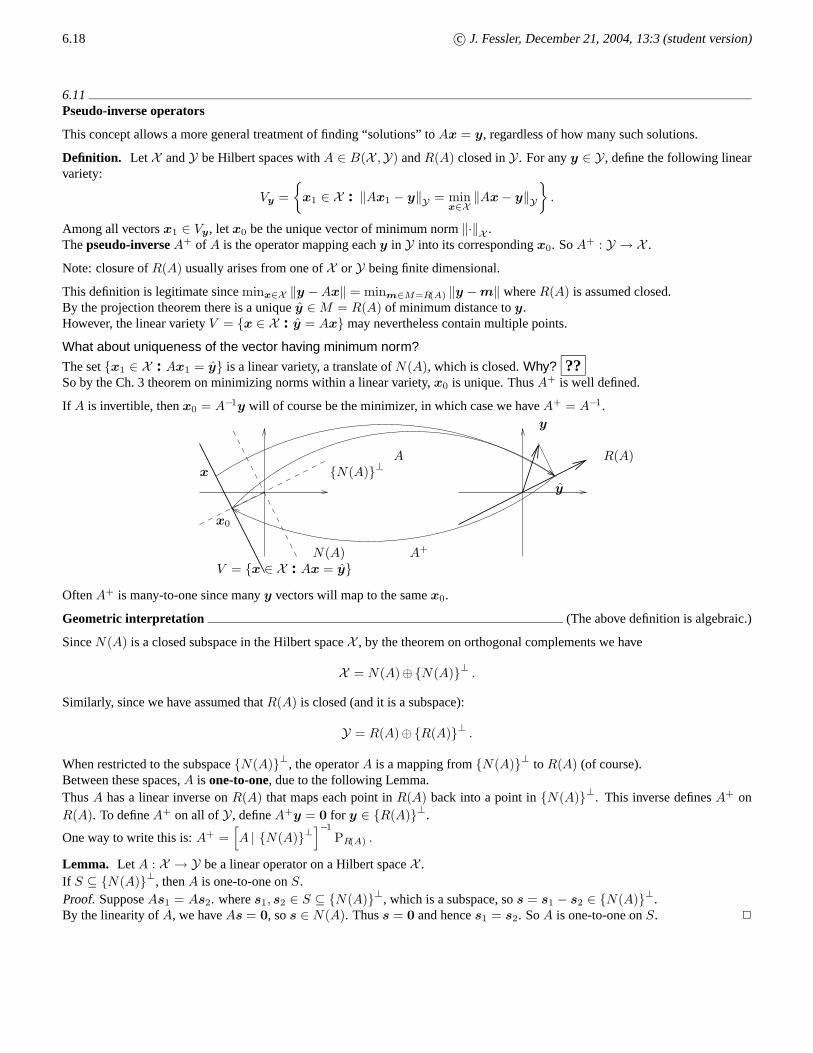
Definition. Let X andY be Hilbert spaces withA ∈ B(X ,Y) andR(A) closed inY. For anyy ∈ Y, define the following linearvariety:

Vy =

{

x1 ∈ X : ‖Ax1 − y‖Y = minx∈X

‖Ax − y‖Y}

.

Among all vectorsx1 ∈ Vy, let x0 be the unique vector of minimum norm‖·‖X .Thepseudo-inverseA+ of A is the operator mapping eachy in Y into its correspondingx0. SoA+ : Y → X .

Note: closure ofR(A) usually arises from one ofX orY being finite dimensional.

This definition is legitimate sinceminx∈X ‖y − Ax‖ = minm∈M=R(A) ‖y − m‖ whereR(A) is assumed closed.By the projection theorem there is a uniquey ∈ M = R(A) of minimum distance toy.However, the linear varietyV = {x ∈ X : y = Ax} may nevertheless contain multiple points.

What about uniqueness of the vector having minimum norm?

The set{x1 ∈ X : Ax1 = y} is a linear variety, a translate ofN(A), which is closed.Why? ??So by the Ch. 3 theorem on minimizing norms within a linear variety, x0 is unique. ThusA+ is well defined.

If A is invertible, thenx0 = A−1y will of course be the minimizer, in which case we haveA+ = A−1.

A

A+

R(A)

N(A)

{N(A)}⊥x

x0

y

y

V = {x ∈ X : Ax = y}

OftenA+ is many-to-one since manyy vectors will map to the samex0.

Geometric interpretation (The above definition is algebraic.)

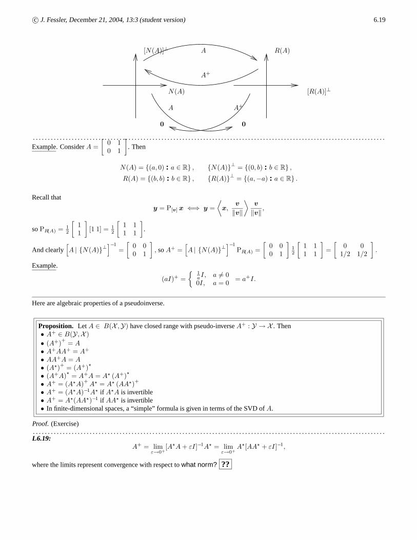
SinceN(A) is a closed subspace in the Hilbert spaceX , by the theorem on orthogonal complements we have

X = N(A)⊕{N(A)}⊥ .

Similarly, since we have assumed thatR(A) is closed (and it is a subspace):

Y = R(A)⊕{R(A)}⊥ .

When restricted to the subspace{N(A)}⊥, the operatorA is a mapping from{N(A)}⊥ to R(A) (of course).Between these spaces,A is one-to-one, due to the following Lemma.ThusA has a linear inverse onR(A) that maps each point inR(A) back into a point in{N(A)}⊥. This inverse definesA+ onR(A). To defineA+ on all ofY, defineA+y = 0 for y ∈ {R(A)}⊥.

One way to write this is:A+ =[

A | {N(A)}⊥]−1

PR(A) .

Lemma. Let A : X → Y be a linear operator on a Hilbert spaceX .If S ⊆ {N(A)}⊥, thenA is one-to-one onS.Proof.SupposeAs1 = As2. wheres1, s2 ∈ S ⊆ {N(A)}⊥, which is a subspace, sos = s1 − s2 ∈ {N(A)}⊥.By the linearity ofA, we haveAs = 0, sos ∈ N(A). Thuss = 0 and hences1 = s2. SoA is one-to-one onS. 2


A

A A+

A+

00

R(A)

[R(A)]⊥

[N(A)]⊥

N(A)

. . . . . . . . . . . . . . . . . . . . . . . . . . . . . . . . . . . . . . . . . . . . . . . . . . .. . . . . . . . . . . . . . . . . . . . . . . . . . . . . . . . . . . . . . . . . . . . . . . . . . .. . . . . . . . . . . . . . . .Example. ConsiderA =

[0 10 1

]

. Then

N(A) = {(a, 0) : a ∈ R} , {N(A)}⊥ = {(0, b) : b ∈ R} ,

R(A) = {(b, b) : b ∈ R} , {R(A)}⊥ = {(a,−a) : a ∈ R} .

Recall that

y = P[v] x ⇐⇒ y =

⟨

x,v

‖v‖

⟩v

‖v‖ ,

soPR(A) = 12

[11

]

[1 1] = 12

[1 11 1

]

.

And clearly[

A | {N(A)}⊥]−1

=

[0 00 1

]

, soA+ =[

A | {N(A)}⊥]−1

PR(A) =

[0 00 1

]

12

[1 11 1

]

=

[0 0

1/2 1/2

]

.

Example.

(aI)+ =

{1aI, a 6= 00I, a = 0

= a+I.

Here are algebraic properties of a pseudoinverse.

Proposition. Let A ∈ B(X ,Y) have closed range with pseudo-inverseA+ : Y → X . Then• A+ ∈ B(Y,X )

• (A+)+

= A• A+AA+ = A+

• AA+A = A• (A?)

+= (A+)

?

• (A+A)?

= A+A = A? (A+)?

• A+ = (A?A)+

A? = A? (AA?)+

• A+ = (A?A)−1A? if A?A is invertible• A+ = A?(AA?)−1 if AA? is invertible• In finite-dimensional spaces, a “simple” formula is given interms of the SVD ofA.

Proof. (Exercise). . . . . . . . . . . . . . . . . . . . . . . . . . . . . . . . . . . . . . . . . . . . . . . . . . .. . . . . . . . . . . . . . . . . . . . . . . . . . . . . . . . . . . . . . . . . . . . . . . . . . .. . . . . . . . . . . . . . . .L6.19:

A+ = limε→0+

[A?A + εI]−1A? = limε→0+

A?[AA? + εI]−1,

where the limits represent convergence with respect towhat norm? ??


. . . . . . . . . . . . . . . . . . . . . . . . . . . . . . . . . . . . . . . . . . . . . . . . . . .. . . . . . . . . . . . . . . . . . . . . . . . . . . . . . . . . . . . . . . . . . . . . . . . . . .. . . . . . . . . . . . . . . .One property that is missing is(CB)+ 6= B+C+, unlike with adjoints and inverses.

However,L 6.21claims that ifB is onto andC is one-to-one, then(CB)+ = B+C+.

Example.

C = [1 1], C? =

[11

]

, C+ = C? (CC?)−1

=

[1/21/2

]

, B =

[10

]

, B? = [1 0], B+ = (B?B)−1

B? = [1 0].

In this case,CB = 1, butB+C+ = 1/2.

Example. Something involving DTFT/filtering following DTFT analysi s.

Example. Downsampling by averaging. (Handwritten notes.)

Example. (p.165)

From regularization design in tomography, form a LS approximation of the form:f(φ) ≈∑3k=0 αk cos2

(φ − π

4 k).

But thosecos terms are linearly dependent!

More generally, if thexi’s may be linearly dependent. how to we work with

minα∈Cn

∥∥∥∥∥y −

n∑

i=1

αixi

∥∥∥∥∥

.

DefineA : Cn → H by α =

∑ni=1 αixi, wherey,xi ∈ H.

If minimizing α not unique, we could choose the one of minimum norm.HereR(A) is closed since it is a finite-dimensional subspace ofH.SoA+ exists andA+ = (A?A)+A?, whereG = A?A is simply then × n Gram matrix. So the minimum norm LS solution is

α = A+y = (A?A)+A?y.

SinceG is (Hermitian) symmetric nonnegative definite, it has an orthogonal eigenvector decompositionG = QDQ′, and one canshow thatG+ = QD+Q′.


Analysis of the DTFT

Given a discrete-time signalg(n), i.e., g : Z → C, thediscrete-time Fourier transform or DTFT is “defined” in introductorysignal processing books as follows:

G = Fg ⇐⇒ G(ω) =∞∑

n=−∞g(n) e−ıωn . (6-2)

This is an infinite series, so for a rigorous treatment we mustfind suitable normed spaces in which we can establish convergence.

The natural family of norms isp, for some1 ≤ p ≤ ∞. Why? What about the doubly infinite sum? ??

The logical meaning of the above definition is really

G = Fg ⇐⇒ G = limN→∞

FNg, whereGN = FNg ⇐⇒ GN (ω) ,

N∑

n=−N

g(n) e−ıωn , whereN ∈ N. (6-3)

Alternatively, one might also try to show thatF = limN→∞ FN , where the limit is with respect to the operator norm inB(`p,Lr[−π, π]) for somep andr, but this is in fact false! (See below.)• SinceGN (ω) is only a finite sum, clearly it is always well defined.• Furthermore, being a finite sum of complex exponentials,GN (ω) is continuous inω, and hence Lebesgue integrable on[−π, π].

So we could writeFN : R2N+1 → L1[−π, π] or perhaps more usefully:FN : `p → Lr[−π, π] for any1 ≤ p, r ≤ ∞.

To elaborate, note that by Holder’s inequality:

|GN (ω)| =

∣∣∣∣∣

N∑

n=−N

g(n) e−ıωn

∣∣∣∣∣≤

N∑

n=−N

|g(n)| =

∞∑

n=−∞|g(n) 1{|n|≤N}| ≤ ‖g‖p

∥∥∥ 1{|n|≤N}

∥∥∥

q= ‖g‖p (2N + 1)1−1/p.

Thus

‖FNg‖r = ‖GN‖r =

(∫ π

−π

|GN (ω)|r dω

)1/r

≤ (2π)1/r ‖g‖p (2N + 1)1−1/p. (6-4)

Furthermore, forp = 1 the upper bound is achieved wheng(n) = δ[n], so|||FN |||1→r = (2π)1/r.• ThusFN ∈ B(`p,Lr[−π, π]) for any1 ≤ p, r ≤ ∞, and|||FN |||p→r ≤ (2π)1/r(2N + 1)1−1/p.• Remark.f ∈ L∞[a, b] =⇒ f ∈ Lr[a, b] if −∞ < a < b < ∞ andr ≥ 1.

But to make (6-2) rigorous we must have normed spaces in whichthe limit in (6-3) exists.

Non-convergence of the operators

Note: treatingFN : `p → Lr[−π, π], by consideringg0(n) = δ[n − (M + 1)] we have forN > M :

|||FN −FM |||p→r = supg : ‖g‖

p≤1

‖(FN −FM )g‖r ≥ ‖(FN −FM )g0‖r =∥∥∥e−ıω(M−1) − 0

∥∥∥

r= (2π)1/r.

So{FN} is not Cauchy (and hence not convergent) inB(`p,Lr[−π, π]), no matter whatp or r values one chooses.So we must analyze convergence of the spectraGN (ω) = FNg, rather than convergence of the operatorsFN themselves.


`1 analysis

Proposition. If g ∈ `1, then{FNg} is Cauchy inLr[−π, π] for any1 ≤ r ≤ ∞.

Proof.

If g ∈ `1, then definingI(N,M) , {n ∈ Z : min(N,M) < |n| ≤ max(N,M)} (6-5)

andGN = FNg we have

|GN (ω) − GM (ω)| =

∣∣∣∣∣

N∑

n=−N

g(n) e−ıωn −M∑

n=−M

g(n) e−ıωn

∣∣∣∣∣=

∣∣∣∣∣∣

∑

n∈I(N,M)

g(n) e−ıωn

∣∣∣∣∣∣

≤∑

n∈I(N,M)

|g(n)| ≤∑

|n|>min(N,M)

|g(n)| → 0 asN,M → ∞. (6-6)

So for eachω ∈ R, the sequence{GN (ω)}∞N=1 is Cauchy inR, and hence convergent by the completeness ofR, providedg ∈ `1.Thus for eachω, {GN (ω)} converges pointwiseto some limit, call itG(ω), where (6-2) is shorthand for that limit.

Furthermore, wheng ∈ `1:‖GN − GM‖∞ = sup

|ω|≤π

|GN (ω) − GM (ω)| → 0 asN,M → ∞.

So the sequence of function{GN} is Cauchy inL∞[−π, π], which is complete, so{GN} converges to a limitG ∈ L∞[−π, π].

More generally, using (6-6):

‖GN − GM‖rr =

∫ π

−π

|GN (ω) − GM (ω)|r dω ≤ 2π∑

|n|>min(N,M)

|g(n)| → 0 asN,M → ∞,

so{GN} is Cauchy inLr[−π, π] for any1 ≤ r ≤ ∞. 2

. . . . . . . . . . . . . . . . . . . . . . . . . . . . . . . . . . . . . . . . . . . . . . . . . . .. . . . . . . . . . . . . . . . . . . . . . . . . . . . . . . . . . . . . . . . . . . . . . . . . . .. . . . . . . . . . . . . . . .Thus, due to completeness,{GN} converges to a limitG ∈ Lr[−π, π].So we can define the DTFT operatorF : `1 → Lr[−π, π] by

Fg , limN→∞

FNg. (6-7)

Proposition. F ∈ B(`1,Lr[−π, π]) for any1 ≤ r ≤ ∞ with |||F|||1→r = (2π)1/r.

Proof.Linearity ofF follows from linearity ofFN . Forg ∈ `1:

‖Fg‖r =∥∥∥ lim

N→∞FNg

∥∥∥

r= lim

N→∞‖FNg‖r ≤ lim

N→∞|||FN |||1→r ‖g‖1 = (2π)1/r ‖g‖1 ,

using (6-4). Equality is achieved wheng(n) = δ[n]. 2


`2 analysis

Unfortunately, 1 analysis is a bit restrictive; the class of signals is not as broad as we might like, and for least-squares problemswe would rather work in2. This will allow us to apply Hilbert space methods.

However, if a signal is in2, it is not necessarily in1, so the above1 analysisdoes not applyto many signals in2. So we need adifferent approach.

Proposition. If g ∈ `2, then{FNg} is Cauchy inL2[−π, π].

Proof. If g ∈ `2,then usingGN = FNg:

‖GN − GM‖22 =

∫ π

−π

∣∣∣∣∣

N∑

n=−N

g(n) e−ıωn −M∑

n=−M

g(n) e−ıωn

∣∣∣∣∣

2

dω =

∫ π

−π

∣∣∣∣∣

∑

n∈I(N,M)

g(n) e−ıωn

∣∣∣∣∣

2

dω

=∑

n∈I(N,M)

∑

m∈I(N,M)

g(n)g∗(m)

∫ π

−π

e−ıω(n−m) dω =∑

n∈I(N,M)

∑

m∈I(N,M)

g(n)g∗(m)2π 1{n=m}

= 2π∑

n∈I(N,M)

|g(n)|2 ≤ 2π∑

|n|>min(N,M)

|g(n)|2 → 0 asN,M → ∞,

sinceg ∈ `2. Thus{FNg} is Cauchy inL2[−π, π]. 2

SinceL2[−π, π] is complete,{GN} is convergent (in theL2 sense!) to some limitG ∈ L2[−π, π], and the expression in (6-2) isagain a reasonable “shorthand” for that limit, whatever it may be, and now we can defineF : `2 → L2[−π, π] via (6-7). In otherwords,

‖GN − GM‖22 =

∫ π

−π

|GN (ω) − G(ω)|2 dω → 0.

This is often calledmean squareconvergence.

Proposition. F ∈ B(`2,L2[−π, π]) with |||F|||2→2 =√

2π.

Proof.Linearity ofF is easily shown.Since{GN} is convergent it is bounded. In fact

‖GN‖22 =

∫ π

−π

∣∣∣∣∣

N∑

n=−N

g(n) e−ıωn

∣∣∣∣∣

2

dω =

N∑

n=−N

N∑

m=−N

g(n)g∗(m)

∫ π

−π

e−ıω(n−m) dω = 2π

N∑

n=−N

|g(n)|2 ≤ 2π ‖g‖22 ,

so‖Fg‖2 ≤√

2π ‖g‖2 and hence|||F||| ≤√

2π.

Furthermore, if we considerg(n) = δ[n], thenG(ω) = 1.Thus‖G‖2

2 =∫ π

−π1 dω = 2π which achieves the upper bound above. Hence|||F|||2→2 =

√2π. 2


Adjoint

SinceF ∈ B(`2,L2[−π, π]) and both 2 andL2[−π, π] are Hilbert spaces,F has an adjoint:

〈Fg, S〉L2[−π,π] =

∫ π

−π

S∗(ω)

(∑

n

g(n) e−ıωn

)

dω =∑

n

g(n)

(∫ π

−π

S(ω) eıωn dω

)∗= 〈g, F?S〉`2

wherex = F?S ⇐⇒ x(n) =∫ π

−πS(ω) eıωn dω, ∀n ∈ Z.

So the adjoint is almost the same as the inverse DTFT (defined below).

And of course we know thatF? ∈ B(L2[−π, π], `2).

Range

To apply the Hilbert space methods, we would likeR(F) to be closed inL2[−π, π]. It suffices forR(F) to be ontoL2[−π, π],since of courseL2[−π, π] itself is closed.

Proposition. The DTFTF : `2 → L2[−π, π] defined by (6-2) isontoL2[−π, π].

Proof.Let ek, k ∈ Z denote the family of functionsek(ω) = 1√2π

e−ıωk.

Recall that{ek} is acomplete orthonormal basisfor L2[−π, π] [4, p. 62].

Thus, byParseval’s relationwe have for anyG ∈ L2[−π, π]:

G =∑

k

〈G, ek〉 ek, i.e., G(ω) =∑

k

〈G, ek〉1√2π

e−ıωk ,

where ∑

k

| 〈G, ek〉 |2 = ‖G‖22 .

Thus if we defineg(k) = 〈G, ek〉 /√

2π theng ∈ `2 andG = Fg, soG ∈ R(F).SinceG ∈ L2[−π, π] was arbitrary, we concludeR(F) = L2[−π, π]. 2

DTFT is (almost) unitary

One can show easily that〈Fu, Fv〉L2[−π,π] = 2π 〈u, v〉2 .

Thus (sinceF is linear and invertible and hence an isomorphism), the normalized DTFTU = 1/√

2πF is unitary.

SoL2[−π, π] and`2 are unitarily equivalent.


Inverse DTFT

Define a “partial inverse DTFT” operatorRN : L2[−π, π] → `2 by

gN = RNG ⇐⇒ gN (n) =1

2π

∫ π

−π

G(ω) eıωn dω 1{|n|≤N} =1√2π

〈G, en〉 1{|n|≤N}.

Proposition. If G ∈ L2[−π, π], then{RNG} is Cauchy in 2.

Proof.

‖RNG −RMG‖ =1

2π

∑

k∈I(N,M)

| 〈G, ek〉 |2 ≤ 1

2π

∑

|k|>min(N,M)

| 〈G, ek〉 |2 → 0 asN,M → ∞.

2

Since`2 is complete,{RNG} converges to some limitg ∈ `2 and we defineRG to be that limit:RG , limN→∞ RNG.

Proposition. R ∈ B(L2[−π, π], `2) and|||R||| = 1/√

2π.

Proof.

‖RNG‖22 =

∑

|n|≤N

∣∣∣∣

1

2π

∫ π

−π

G(ω) eıωn dω

∣∣∣∣

2

=1

2π

∑

|k|≤N

| 〈G, ek〉 |2 ≤ 1

2π

∑

k

| 〈G, ek〉 |2 =1

2π‖G‖2

2 .

So |||RN ||| ≤ 1/√

2π andRN ∈ B(L2[−π, π], `2).WhenG(ω) = 1 we have‖RNG‖2

= ‖δ[n]‖2= 1 and‖G‖2

= 2π so|||RN ||| = 1/√

2π.

Proof 2.‖RG‖2 = limN→∞ ‖RNG‖2 ≤ limN→∞1√2π

‖G‖2 . ConsiderG = 1 to show equality. 2

Proposition. RF = I`2 andFR = IL2, soF−1 = R, whereIH denotes the identity operator for Hilbert spaceH.

Proof.Exercise. 2


Convolution revisited

Using time-domain analysis, we showed previously that ifh ∈ `1 andAx = h ∗ x thenA ∈ B(`p, `p).

We have shownF ∈ B(`2,L2[−π, π]) andF−1 ∈ B(L2[−π, π], `2).Consider the “band-limiting” linear operatorD : L2[−π, π] → L2[−π, π] defined by

y = Dx ⇐⇒ y(ω) =

{x(ω), |ω| ≤ π/20, otherwise.

ClearlyD ∈ B(L2[−π, π],L2[−π, π]) and in fact|||D||| = 1.

Now considerA , F−1DF . We previously showed in the analysis of the composition of operators that|||ST ||| ≤ |||S||||||T |||.SoA ∈ B(`2, `2) with |||A||| ≤ |||F−1||||||D||||||F||| ≤ 1√

2π· 1 ·

√2π = 1.

But thisA represents an ideal lowpass filter,i.e., convolution withh(n) = 12 sinc

(n2

). But thish /∈ `1.

Evidently, the convolution operator, at least in`2, has a looser requirement thanh ∈ `1.

In contrast, in ∞, h ∈ `1 is both necessary and sufficient forAh ∈ B(`∞, `∞).

In `2, a necessary and sufficient condition is that the frequency response be bounded.

Proposition. Ah ∈ B(`2, `2) (with |||Ah||| = ‖H‖∞) ⇐⇒ ‖Fh‖∞ < ∞, i.e.,Fh ∈ L∞[−π, π] .

Proof. (⇐=) Suppose‖Fh‖∞ is finite. Then using the convolution property of the DTFT andParseval:

‖h ∗ x‖22 =

1

2π‖HX‖2

2 =1

2π

∫ π

−π

|H(ω)X(ω)|2 dω ≤ ‖H‖2∞

1

2π‖X‖2

2 = ‖H‖2∞ ‖x‖2

2 ,

|||Ah||| ≤ ‖Fh‖∞ = ‖H‖∞ . The upper bounded is achieved whenh(n) = δ[n].

(=⇒) If H is unbounded, then forallT there exists an interval over whichH ≥ T . Choosex to be a signal whose spectrum is anindicator function on that interval, and then‖x ∗ h‖2 ≥ T ‖x‖2, soAh would be be unbounded. Take contrapositive. 2

Continuous-time case

Fourier transform

convolution

Young’s inequality

c© J. Fessler, December 21, 2004, 13:3 (student version)

1. P. Enflo. A counterexample to the approximation problem inBanach spaces.Acta Math, 130:309–17, 1973.2. I. J. Maddox.Elements of functional analysis. Cambridge, 2 edition, 1988.3. A. W. Naylor and G. R. Sell.Linear operator theory in engineering and science. Springer-Verlag, New York, 2 edition, 1982.4. D. G. Luenberger.Optimization by vector space methods. Wiley, New York, 1969.5. J. Schauder. Zur theorie stetiger abbildungen in funktionenrumen.Math. Zeitsch., 26:47–65, 1927.6. L. Grafakos.Classical and modern Fourier analysis. Pearson, NJ, 2004.7. P. P. Vaidyanathan. Generalizations of the sampling theorem: Seven decades after Nyquist.IEEE Tr. Circ. Sys. I, Fundamental

theory and applications, 48(9):1094–109, September 2001.8. A. M. Ostrowski.Solution of equations in Euclidian and Banach spaces. Academic, 3 edition, 1973.9. R. R. Meyer. Sufficient conditions for the convergence of monotonic mathematical programming algorithms.J. Comput.

System. Sci., 12(1):108–21, 1976.10. M. Rosenlicht.Introduction to analysis. Dover, New York, 1985.11. A. R. De Pierro. On the relation between the ISRA and the EMalgorithm for positron emission tomography.IEEE Tr. Med.

Imag., 12(2):328–33, June 1993.12. A. R. De Pierro. On the convergence of the iterative imagespace reconstruction algorithm for volume ECT.IEEE Tr. Med.

Imag., 6(2):174–175, June 1987.13. A. R. De Pierro. Unified approach to regularized maximum likelihood estimation in computed tomography. InProc. SPIE

3171, Comp. Exper. and Num. Meth. for Solving Ill-Posed Inv.Imaging Problems: Med. and Nonmed. Appl., pages 218–23,1997.

14. J. A. Fessler. Grouped coordinate descent algorithms for robust edge-preserving image restoration. InProc. SPIE 3170, Im.Recon. and Restor. II, pages 184–94, 1997.

15. A. R. De Pierro. A modified expectation maximization algorithm for penalized likelihood estimation in emission tomography.IEEE Tr. Med. Imag., 14(1):132–137, March 1995.

16. J. A. Fessler and A. O. Hero. Penalized maximum-likelihood image reconstruction using space-alternating generalized EMalgorithms.IEEE Tr. Im. Proc., 4(10):1417–29, October 1995.

17. M. W. Jacobson and J. A. Fessler. Properties of MM algorithms on convex feasible sets.SIAM J. Optim., 2003. Submitted. #061996.

18. P. L. Combettes and H. J. Trussell. Method of successive projections for finding a common point of sets in metric spaces. J.Optim. Theory Appl., 67(3):487–507, December 1990.

19. F. Deutsch. The convexity of Chebyshev sets in Hilbert space. In A. Yanushauskas Th. M. Rassias, H. M. Srivastava, editor,Topics in polynomials of one and several variables and theirapplications, pages 143–50. World Sci. Publishing, River Edge,NJ, 1993.

20. M. Jiang. On Johnson’s example of a nonconvex Chebyshev set. J. Approx. Theory, 74(2):152–8, August 1993.21. V. S. Balaganskii and L. P. Vlasov. The problem of convexity of Chebyshev sets.Russian Mathematical Surveys, 51(6):1127–

90, November 1996.22. V. Kanellopoulos. On the convexity of the weakly compactChebyshev sets in Banach spaces.Israel Journal of Mathematics,

117:61–9, 2000.23. A. R. Alimov. On the structure of the complements of Chebyshev sets.Functional Analysis and Its Applications, 35(3):176–

82, July 2001.24. Y. Bresler, S. Basu, and C. Couvreur. Hilbert spaces and least squares methods for signal processing, 2000. Draft.25. M. Vetterli and J. Kovacevic.Wavelets and subband coding. Prentice-Hall, New York, 1995.26. D. C. Youla and H. Webb. Image restoration by the method ofconvex projections: Part I—Theory.IEEE Tr. Med. Imag.,

1(2):81–94, October 1982.27. M. Unser and T. Blu. Generalized smoothing splines and the optimal discretization of the wiener filter.IEEE Tr. Sig. Proc.,

2004. in press.

linear operators and adjoints - university of michiganfessler/course/600/l/l06.pdf · 6.2 c j....

Documents