linear mixed-effects models for estimating biomass and fuel loads in shrublands

Linear mixed-effects models for estimatingbiomass and fuel loads in shrublands

H.G. Pearce, W.R. Anderson, L.G. Fogarty, C.L. Todoroki, and S.A.J. Anderson

Abstract: Shrubland biomass is important for fire management programmes and for carbon estimates. Aboveground bio-mass and the combustible portion of biomass, the fuel load, in the past have been measured using destructive techniques.These techniques are detailed, highly labour intensive, and costly; hence, an alternative approach was sought. The new ap-proach used linear mixed-effects models to estimate biomass and fuel loads from easily measured field variables: shruboverstorey height and cover, and understorey height and cover. Site was regarded as a random effect. Sampling sites werelocated throughout New Zealand and included a range of shrubland vegetation types: manuka (Leptospermum scopariumJ.R. Forst. et G. Forst.) and kanuka (Kunzea ericoides (A. Rich.) J. Thomps.) scrub and heath, pakihi (mixed low heath,fern, and rushes), and gorse (Ulex europaeus L.). The approach was extended and confidence intervals were constructedfor the regression models. Statistical analysis showed that understorey height and overstorey cover were significant (at the5% level) in some cases. Overstorey height was highly significant in all cases (p < 0.0001), allowing development of mod-els useful to the operational user. The models allow rapid estimation of average fuel loads or biomass on new sites, anddouble sampling theory can be applied to calculate the error in the resultant biomass estimate.

Resume : La biomasse des arbustaies est importante pour les programmes de gestion du feu et pour les estimations du car-bone. La biomasse aerienne et la portion combustible de la biomasse, la charge de combustibles, ont dans le passe ete me-surees a l’aide de techniques destructives. Ces techniques sont minutieuses, exigeantes en main d’œuvre et couteuses. Parconsequent, nous avons cherche une approche alternative. La nouvelle approche utilise des modeles lineaires a effets mix-tes pour estimer la biomasse et les charges de combustibles a partir de variables facilement mesurables sur le terrain : lahauteur et le couvert de l’etage dominant arbustif ainsi que la hauteur et le recouvrement de la vegetation de sous-bois. Lastation a ete consideree comme un effet aleatoire. Les sites d’echantillonnage etaient reparties a travers la Nouvelle-Ze-lande et incluaient une variete de types vegetaux arbustifs : les broussailles et les landes a manuka (Leptospermum scopa-rium J.R. Forst et G. Forst) et a kanuka (Kunzea ericoides (A. Rich.) J. Thomps.), le pakihi (lande humide recouverte d’unmelange de fougeres et de roseaux) et l’ajonc d’Europe (Ulex europaeus L.). L’approche a ete elargie et des intervalles deconfiance ont ete elabores pour les modeles de regression. L’analyse statistique a montre que la hauteur de la vegetationde sous-bois et le couvert de l’etage dominant etaient des variables significatives (au niveau de 5 %) dans certains cas. Lahauteur de l’etage dominant etait une variable tres significative (p < 0,0001) dans tous les cas, ce qui a permis de develop-per des modeles utiles pour un utilisateur operationnel. Les modeles permettent d’obtenir une estimation rapide des chargesde combustibles ou de la biomasse dans les nouveaux sites et la theorie du double echantillonnage peut etre appliqueepour calculer l’erreur de l’estimation de la biomasse ainsi obtenue.

[Traduit par la Redaction]

IntroductionThe study of aboveground available fuel (AGAF), in

terms of quantity and structure, is central to fire researchand management programmes because of the effect that fuel

load has on fire behaviour. Frontal fire intensity, which de-scribes the rate of energy or heat release per unit length offire front (Byram 1959), is directly proportional to fuel load(Alexander 1982) and is determined from the fuel’s heat ofcombustion, the fire rate of spread, and the amount of fuelconsumed by the fire — essentially the AGAF (or a propor-tion thereof). Key fire management decisions relating to firesuppression (as determined by fire intensity) and prepared-ness require knowledge of fuel loadings. Accurate estima-tion of available fuel loads for different vegetation types istherefore essential for safe and effective fire management.

AGAF represents the combustible portion of total above-ground biomass (TAGB). Measurement of biomass (bothaboveground and belowground) is common for forest vege-tation (e.g., Fehrmann et al. 2008; Basuki et al. 2009), andin recent years, estimation of total biomass has become in-creasingly important for carbon accounting and for identifi-cation of potential sources of renewable energy (Kirschbaum2003) in other vegetation types, including shrublands.

Received 21 December 2009. Accepted 29 June 2010. Publishedon the NRC Research Press Web site at cjfr.nrc.ca on24 September 2010.

H.G. Pearce1 and S.A.J. Anderson. Scion, P.O. Box 29-237,Fendalton, Christchurch 8540, New Zealand.W.R. Anderson. University of New South Wales at ADFA,Canberra, ACT 2600, Australia.L.G. Fogarty. Department of Sustainability and Environment,Fire and Emergency Management Division, P.O. Box 500, EastMelbourne, Victoria 3002, Australia.C.L. Todoroki. Scion, Private Bag 3020, Rotorua 3046, NewZealand.

1Corresponding author (e-mail:[email protected]).

2015

Can. J. For. Res. 40: 2015–2026 (2010) doi:10.1139/X10-139 Published by NRC Research Press

Shrubland communities, which account for around 40% ofthe total annual area burned in fires (Anderson et al. 2008),cover some 7.5 million hectares, about 28%, of New Zea-land (Newsome 1987). From a fire management standpoint,the important shrubland vegetation types include manuka(Leptospermum scoparium J.R. Forst. & G. Forst.) and ka-nuka (Kunzea ericoides (A. Rich.) J. Thomps.) scrub andheath, native pakihi wetland (mixed low heath, ferns, andrushes dominated by Baumea teretifolia (R.Br.) Palla), andthe exotic scrub weed gorse (Ulex europaeus L.), whichcovers approximately 700 000 ha (or almost 3% of the landarea of the country) (Blaschke et al. 1981). Gorse, manuka,and kanuka scrub are dense plants with a continuous ornear-continuous canopy cover. Pakihi, on the other hand, aMaori word that originally meant open country, is an openshrub wetland.

In the past, measurements of available fuel loads and totalbiomass of shrubland vegetation have been made using tech-niques similar to those described by Brown et al. (1982) fordestructive sampling of herbaceous vegetation and litter. De-structive sampling involves locating sampling points, estab-lishing quadrats, taking inventory of plant material withineach quadrat, and cutting and bagging the vegetation forsubsequent sorting, drying, and weighing in a laboratory.The vegetation may also be classified according to strata,such as shrub overstorey, understorey, litter, and duff (fer-mentation and humus layers). This stratification is usedwithin the New Zealand Fire Fuels Database (Manning andPearce 2008), which includes data collected in conjunctionwith fire behaviour experiments, wildfires, biomass assess-ment (e.g., for carbon), and other fire research activities.

Fuel loads and (or) biomass may also be estimatedthrough nondestructive sampling methods, such as line orplanar intersect sampling (Shiver and Borders 1996), visualor ocular estimation and photoguides (Fischer 1981; Keaneand Dickinson 2007), and hazard scoring (Cruz et al. 2010).More recently ground-based laser ranging has been used tocapture shrub fuel characteristics important for determiningfire behaviour and to compare nondestructive with destruc-tive measurements (Loudermilk et al. 2009).

Regression equations, formulated between biomass or fuelload, and easily measured independent variables, such asheight or cover, form the basis of the statistical methodknown as double sampling (Shiver and Borders 1996). Themethod is advantageous in that the regression equations canbe applied to new sites by taking multiple measurementsalong transects and by determining the averages of the inde-pendent variables to give an estimate of the average biomasson the site. A confidence interval for this estimate can thenbe constructed using double sampling theory. The doublesampling method has been shown to be cost-efficient whenused for estimating vegetation biomass (Catchpole andCatchpole 1993), in comparison with other direct samplingtechniques (Catchpole and Wheeler 1992).

Pereira et al. (1995), for example, developed nonlinear re-gression models based on dimensional analysis to predict bi-omass from structural measurements of shrubs inMediterranean regions, where undergrowth within foreststands of shrub fuels is of major importance. For UnitedStates vegetation types, Means et al. (1996) modified the BI-OPAK software package (Means et al. 1994) to include a li-

brary of double sampling equations for estimating thebiomass of shrubs and herbs.

The methods (destructive versus nondestructive) differ inthe levels of accuracy and expertise required, but the morecomplex and time-consuming destructive methods generallydeliver higher levels of accuracy than the nondestructive al-ternatives (Catchpole and Wheeler 1992).

The New Zealand Fire Fuels Database has been used todevelop preliminary models for estimating fuel loads and bi-omass (Fogarty and Pearce 2000; Pearce and Anderson2008). The models are based on logarithmic regressions andare of the form given by eq. 1, commonly used in biomassestimations (Baskerville 1972; Meng et al. 2007), or of theequivalent allometric form often used in other biological ap-plications (West et al. 1997) given by eq. 2.

½1� ln ðyÞ ¼ ln ðaÞ þ bln ðxÞ

½2� y ¼ axb

where y represents fuel load and x represents height, percentcover, or a combination of the two, and a and b are con-stants.

Models in the form of eqs. 1 or 2 commonly use diameterat breast height as the sole independent variable to estimateaboveground biomass in forests (e.g., Basuki et al. 2009) orshrub communities (Brown 1976; De Luis et al. 2004). Itshould be noted that estimates obtained using eq. 1 requirea correction for the bias that is introduced by the logarithmictransformation itself (Baskerville 1972), and that these esti-mates ignore any ‘‘group effects’’, such as species or sitequality. In addition, there may be random group effects,such as site effects, that are part of the experimental varia-bility, so both within- and between-group variability needsto be modelled.

Between- and within-group variability can be estimatedthrough the application of linear mixed-effects models andparameterization techniques, such as the method of re-stricted maximum likelihood (REML) (Searle et al. 1992).REML can provide estimates of parameters for models thathave more than one source of error, for example, wherethere is variation between quadrats on the same site and var-iation between sites.

The aim of this work was to develop a new approach forestimating biomass (or fuel loads) from quadrat measure-ments of shrubland vegetation. The approach uses linear ef-fects models. These models have recently been applied toestimate tree biomass from satellite images (Meng et al.2007). The novelty of the approach used here stems notonly from the application of mixed-effects models to de-velop regression equations for estimating shrub biomass butalso from the derivation and construction of confidence in-tervals for those equations.

Methods

Vegetative samplesSample data were obtained from sites extending from In-

vercargill (latitude 46.358S, longitude 168.188E) at the bot-tom of the South Island to Tokerau Beach (latitude 34.888S,longitude 173.388E) at the top of the North Island (Fig. 1),

2016 Can. J. For. Res. Vol. 40, 2010

Published by NRC Research Press

spanning the majority of climatic zones within New Zealand(New Zealand Meteorological Service 1983). The data werepredominantly collected in conjunction with fire experi-ments, but were also collected from biomass sampling andwildfire documentation studies. The vegetation typessampled were manuka and kanuka scrub and heath, pakihi(mixed low heath, fern, rush), and gorse. Since manuka andkanuka are very similar species with similar structures andproperties and are often found together, henceforth the man-uka–kanuka vegetation types will be referred to simply asmanuka. Photographs of these vegetation types are providedin Fig. 2.

Using the vegetation structure classification of Specht(1970) based on height and cover, gorse vegetation(Fig. 2a) can be described as either closed or open scrub de-pending on the degree of canopy cover. Manuka vegetationwas divided into scrub and heath, primarily dependent onheight and structure (after Specht 1970) but also on age andsite quality. Manuka scrub (Fig. 2b) would generally also beclassified as either closed or open scrub; however, withmore of a tree form, the tallest manuka scrub sites could beclassed as low open forest, and the sites with lower cover aslow shrubland. In contrast, the manuka heath vegetation(Fig. 2c) would be described as closed heath due to its

shorter stature, higher cover, and predominantly sedgeunderstorey (Shoenus or Baumea spp.). Pakihi vegetation(Fig. 2d) would be classified as sedgeland or, where sparselow heath is present, as low shrubland.

Plots for experimental burning were generally located onflat ground (to remove the influence of slope on fire behav-iour) within continuous fuels of uniform age, structure, andhomogeneity. A number of burn plots were located withinthe same general area (or site). Fuel sampling quadrats werelocated at the corners of the plots selected for burning or atregular intervals along transects (Fig. 3).

At each sampling point, a quadrat was established andphotographed, and measurements were made of averageheight and cover (Fig. 4a) of the overstorey (shrub layer),understorey, and litter layer using a fuelbed strata classifica-tion analogous to that of Sandberg et al. (2001). The downwoody fuel component was generally absent. Ground fuels(soil organic layers) were highly variable but, althoughmeasured when present, were not considered here as part ofthe aboveground biomass. A quadrat size of 4 m � 1 m,comprising four adjoining 1 m � 1 m ‘‘subquadrats’’, wasutilized in an effort to overcome variability in vegetationcover associated with the presence of individual shrubs.

Overstorey height for each 1 m � 1 m subquadrat was de-termined by averaging measurements of the tallest andshortest clumps of fuel (isolated shrubs that were clearlynot part of the main overstorey fuel component wereignored). The percentage cover of the shrub canopy layerwas estimated by assessing the net proportion of each sub-quadrat covered by the vegetation. Similar estimates of aver-age height and cover were also made for understoreyvegetation (combined grasses, herbs, or forbs) and of surfacelitter depth and cover within each subquadrat. The meanheight or depth and percentage cover from each 1 m � 1 msubquadrat were then averaged to provide a single estimatefor each 4 m � 1 m quadrat.

From each quadrat, the elevated overstorey fuel layer wasdestructively sampled first, followed by understorey vegeta-tion then surface litter (Fig. 4b). All the vegetative materialfrom the entire quadrat was harvested, sorted by visual in-spection into live and dead fuel material, and further sortedaccording to diameter classes using a ‘‘go/no-go’’ gauge(Brown 1974). This gauge divided the fuels into size classesbased upon diameter (£0.49, 0.5–0.99, 1.0–2.99, and‡3.0 cm) (after McRae et al. 1979).

Fuel loads and biomass were determined by oven-dryingsamples at 65 8C until all moisture was removed and wereexpressed in kilograms per square metre. While TAGB in-cludes all live and dead matter from the overstorey andunderstorey layers as well as surface litter, AGAF is calcu-lated only from the aboveground fuels, which are responsi-ble for propagating fire. In New Zealand, AGAF iscalculated as the sum of dead overstorey, understorey, andlitter material with a diameter <0.5 cm, and a proportion ofthe live overstorey and understorey vegetation <0.5 cm di-ameter. This is because not all of this live fine material isconsumed by fire. Adjustment factors of 0.81 for gorse,0.76 for manuka, and 1.00 for pakihi are used to estimatethe proportion of these live fine fuels that are actually con-sumed. These factors were derived from measurements ofthe minimum postburn diameters of live twigs remaining

Fig. 1. Location of shrubland biomass sampling sites within NewZealand.

Pearce et al. 2017


following experimental burns in shrubland fuels, whichfound that only material up to 0.2–0.3 cm in diameter wasconsumed. Similar findings have been reported for Austral-ian shrub fuels (Whight and Bradstock 1999). All of thelive material present in pakihi vegetation is <0.5 cm in di-ameter.

Linear mixed-effects modelsThe dependent variables in the analysis were AGAF or

TAGB, and the independent variables were obtained fromquadrat measurements of destructively sampled shrub vege-tation using the methods of Brown et al. (1982). The meas-ured variables were overstorey height (OsHt), overstorey

cover (OsCo), understorey height (UsHt), and understoreycover (UsCo). Typically, there was no understorey associ-ated with the gorse samples, thus the understorey variableswere relevant only for manuka and pakihi. The pakihi fueltype was assigned to the shrubland fuel category (ratherthan grassland), since exploratory analysis showed that pak-ihi fitted better as a shrubland fuel. This is reasonable giventhat pakihi vegetation often represents a successional stagein the transition to shrubland cover. Vegetation type (gorse,manuka, and (or) pakihi) was tested for significance, and thenonsignificant types (p > 0.05) were combined. Separateanalyses were carried out on different combined vegetationtypes, as their load and biomass could potentially be af-

Fig. 2. Illustrative examples of the different New Zealand shrubland vegetation types: (a) gorse, (b) manuka scrub, (c) manuka heath, and(d) pakihi.

Fig. 3. Layout of fuel sampling transects and destructive fuel sampling quadrats located at the corners of the plots selected for burning or atregular intervals along transects.

2018 Can. J. For. Res. Vol. 40, 2010


fected by different independent variables. Within combinedvegetation types (scrub and heath), structure was regardedas a factor.

Samples from two randomly selected sites were removedfor limited validation of the models, one from the manukascrub sites (Torlesse) and the other from the gorse sites(Dunedin). The Torlesse manuka site was also used to illus-trate the double sampling technique (see Results section).Sample sizes and summary statistics for the model and vali-dation sets are provided in Table 1.

The simplest form of the linear mixed-effects model, withfixed effects b0 and b1 and random effects due to site hj andquadrat 3ij, is

½3� yij ¼ b0 þ b1xij þ hj þ 3ij

where yij is a (possible) transformation of AGAF (or TAGB)on the ith quadrat of the jth site, xij is a (possible) transfor-mation of the independent variable on the ith quadrat of thejth site, hj is the random site effect of site j, and 3ij is therandom effect of quadrat i within site j.

The random effects 3ij and hj are assumed to be normallydistributed with zero means and variances, s2

3 and s2h, re-

spectively.Functions that transform AGAF (or TAGB) and the inde-

pendent variables (predominantly natural logarithms, butalso square roots) were determined through inspection ofthe plots to select transforming functions that resulted in lin-earity and constant variance with increasing mean values of

the dependent variable. For simplicity, the slope of the re-gression equation was assumed to be the same for all sites(Note: allowing for different slopes was considered, but theresulting REML estimation procedure did not always con-verge).

An extended form of the model in eq. 3 is

½4� yij ¼ b0 þXp

k¼1

bkxijk þ hj þ 3ij

with bk the coefficient of xijk, the kth independent variable (k= 1, 2, 3, . . ., p) associated with quadrat i on site j.

A factor, such as vegetation group (type or structure), canbe incorporated into the model by using dummy variables.For eqs. 5 and 6, I = 1 for vegetation group 1, and 0 other-wise. In eq. 5, with two vegetation groups and one inde-pendent variable, only the intercept is different for differentvegetation groups, so the regression equations are parallellines. In eq. 6, both the slope and intercept are different fordifferent vegetation groups, so the regression equations arenonparallel lines.

½5� yij ¼ b0 þ b1xij þ b2I þ hj þ 3ij

½6� yij ¼ b0 þ b1xij þ b2I þ b3Ixij þ hj þ 3ij

where the suffix k has been dropped for convenience.Linear mixed-effects models were fitted using the method

of REML. This method was used rather than using site aver-

Fig. 4. Sampling in manuka scrub: (a) estimating average canopy height and (b) collecting surface litter fuels following removal of theelevated fuel layers.

Table 1. Summary statistics (mean with standard deviation in parentheses) of data used in modelling and validation.

Model Validation

Variable*Gorse(n = 55)

Pakihi heath(n = 10)

Manuka heath(n = 22)

Manuka scrub(n = 26)

GorseDunedin (n = 3)

Manuka scrubTorlesse (n = 38)

OsHt (m) 2.8 (0.7) 0.3 (0.1) 1.2 (0.7) 3.6 (1.0) 3.1 (0.1) 2.4 (1.1)OsCo (%) 77.(16) 74.(16) 52.(16) 61.(17) 58.(14) 58.(22)UsHt (m) 0.2 (0.1) 1.0 (0.6) 0.6 (0.9) 0.03 (0.06)UsCo (%) 20.(19) 40.(34) 25.(39)TAGB (kg�m–2) 10.4 (3.2) 0.6 (0.2) 3.4 (2.2) 8.9 (3.8) 12.9 (1.9) 6.9 (4.9)AGAF (kg�m–2) 4.2 (1.1) 0.6 (0.2) 2.4 (1.4) 2.6 (0.9) 5.5 (1.7) 2.3 (1.1)

*OsHt, overstorey height; OsCo, overstorey cover; UsHt, understorey height; and UsCo, understorey cover; TAGB, total aboveground biomass;AGAF, aboveground available fuel.

Pearce et al. 2019


ages and ordinary regression models because sampling wasnot random on sites. Modelling was performed using thesoftware R (R Development Core Team 2008), with the lmefunction, using a mixed-effects model with quadrats nestedwithin sites. Conditional t tests and F tests (Pinheiro andBates 2000) were applied to test the significance of individ-ual variables and factors using a significance level of 0.05.When more than one variable was found to be significant,the value of adding the extra variable to the model was con-sidered by comparing the root mean square error (RMSE)and the mean absolute percentage error (MAPE) of the pre-dictions from the resulting equations (as in Fehrmann et al.2008). The predictions were based on the untransformeddata and were predictions for the population. They excludedthe estimated site effects (because in practice the site effectswould be unknown) but included the bias correction factorfrom Snowdon (1991), which is defined as the mean of ob-served values divided by the mean of predicted values. Withthis factor the mean error was identically equal to zero, somean error could not be used in the model comparisons.

Fit statistics were supplemented by normal probabilityplots of residuals and fitted site effects and by the Ander-son–Darling statistic (Anderson and Darling 1952) to testnormality. Diagnostics also included plots of the fitted linefor each site overlaid on the observed values, plots of resid-uals versus fitted values, box plots of standardized residualsby site, and plots of observed versus fitted values.

Prediction intervalsThe population regression line in eq. 4 for a quadrat with

p independent variable values, x0 ¼ ½1; x1; x2; . . . ; xp� (wherei and j have been omitted for simplicity), can be written inmatrix form as

½7� y ¼ x0b

where b is the vector of parameters. The predicted regres-sion line at x = x0 is found by replacing x by x0 and b by

the vector of REML estimates bb. Thusffiffiffiffiffiffiffiffiffiffiffiffiffiffiffiffiffiffiffiffiffiffiffiffix00cov ðbbÞx0

qis the

standard error of the prediction and can be used to formconfidence intervals (Skrondal and Rabe-Hesketh 2009). Asthe sample sizes are reasonably large, asymptotic normalitycan be assumed for the confidence intervals. When predict-ing a quadrat response on a new site with independent vari-ables x0, the variance of the prediction isx00cov ðbbÞx0 þ s2

h þ s23 (Skrondal and Rabe-Hesketh 2009).

In practice, a prediction of my, the site population mean ofthe dependent variable (AGAF or TAGB), on a new site isrequired. For this the prediction is bmy ¼ m0x

bb; wherem0x ¼ ½1;mx1;mx2; . . . ;mxp�, the vector of population sitemeans of the independent variables, and the variance of theprediction is

½8� var ðbmyÞ ¼ m0xcov ðbbÞmx þ s2h

as the extra quadrat variation is not involved. Prediction in-tervals can be determined for my by replacing cov ðbbÞ and s2

h

by their estimates. For simplicity these intervals can be con-structed using normal theory, although this will underesti-mate the interval size slightly since there are only 11 sitesused in developing this model.

The validation data were used to test how well the modelsperformed with data from new sites. That is, a good fitwould be indicated if the predicted site means fall withinthe prediction intervals, and a poor fit otherwise.

Double samplingThe prediction error given above for estimating my on a

new site assumes that the site means of the independent var-iables are known without error. However, in practice theyare generally estimated by taking several measurementsalong transects, and an extra error of approximatelyb0ðcov bmxÞb is introduced into the variance of the estimateof my (Catchpole and Catchpole 1991, 1993). The doublesampling estimate is ~my ¼ bm 0xbb, wherebm 0x ¼ ½1; �x1; �x2; . . . ; �xp� is the vector of means of the inde-pendent variables from transect sampling. Catchpole andCatchpole (1991, 1993) showed that this estimate is asymp-totically normally distributed and that

½9� var ð ~myÞ � m0xcov ðbbÞmx þ s2h þb0cov ðbmxÞb

For example, for eq. 4, b0ðcov bmxÞb ¼ b21var ð�xÞ. In the case of

the model in eq. 6, b0ðcov bmxÞb ¼ ðb21 þ b1b3 þ b2

3Þvar ð�xÞ.Again double sampling prediction intervals can be found usingasymptotic normality theory and by replacing the parametersand variances with their estimates.

The Torlesse manuka validation data were used to illus-trate the double sampling technique and to show how the re-gression equation would be used in practice. Again, a goodfit would be indicated if the predicted values fall within theprediction intervals.

Results

Aboveground available fuelA plot of AGAF against OsHt for all shrubland vegetation

types showed increasing variance with mean level of over-storey height. Improved homogeneity of variance, linearity,and a clear distinction between the three vegetation typeswere obtained in plots of transformed variables, with thelogarithmic transformation of both variables being more sat-isfactory than a square root alternative.

The model in eq. 6 was fitted to the data, where y =ln(AGAF) and x = ln(OsHt), and the group effect was veg-etation type. The vegetation type effect was highly signifi-cant (p < 0.001), but the interaction term was notsignificant. Pakihi was not significantly different frommanuka (at the 5% level), so these two vegetation typeswere combined and then analysed separately from gorse.The structural characteristics of the gorse and manuka–pak-ihi sampled were considerably different (for example, thegorse had little or no understorey), so it was reasonable tohypothesize that the AGAF could be predicted by differentvariables. The manuka–pakihi combination was further splitinto two vegetation types, scrub or heath, depending onheight and structure.

For manuka–pakihi, ln(OsHt) was by far the most signifi-cant variable (p < 0.001) affecting AGAF. Vegetation struc-ture was significant when added to the model (p = 0.03).The interaction between vegetation structure and ln(OsHt)was also significant (p = 0.02), so that the rate of change of

2020 Can. J. For. Res. Vol. 40, 2010


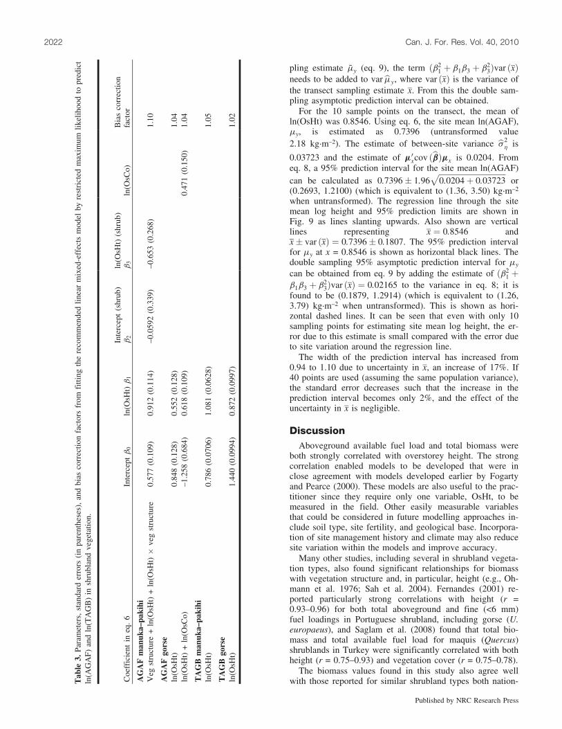
ln(AGAF) with ln(OsHt) was different for the two vegeta-tion types. The only significant correlation between potentialpredictor variables was between understorey height andcover (r = 0.89). Of the other variables that were added tothe model and tested for significance, only UsHt was signif-icant, but it changed the MAPE by only 1% (Table 2). Thus,with diagnostics of the residuals being satisfactory, themodel with ln(OsHt) and the interaction term was the pre-ferred model. The coefficients of the final model and thebias correction are given in Table 3. The intercept for scrubis given by b0 + b0v, and the slope for scrub by b1 + b1v.When exponentiating eq. 6, the right-hand side must be mul-tiplied by the bias correction factor when transforming backto the allometric form of the model.

Figure 5 shows the modelled regression line and 95% pre-diction bands for predictions of AGAF from overstoreyheight (OsHt) for the two manuka–pakihi shrubland struc-tures: (i) heath and pakihi, and (ii) scrub. All site means fallwithin the prediction bands, but it should be noted that thesesite means are not always unbiased estimators of the truesite average. The site mean for the Torlesse validation siteis well within the limits.

For gorse, ln(OsHt) was again the most significant varia-ble (p < 0.001) affecting AGAF. The variable ln(OsCo) wassignificant when added to the model and reduced the MAPEby 3%, but it was significantly negatively correlated withln(OsHt) (r = –0.29, p = 0.03). Understorey fuels were notpresent in the sampled gorse quadrats. Coefficients for mod-els with ln(OsHt) alone and including ln(OsCo) are given inTable 3. The model using ln(OsHt) alone was satisfactory interms of residual analysis and is the recommended model,since the extra precision gained from adding ln(OsCo) isoffset by the difficulty in consistently assessing cover in thefield. Figure 6 shows the modelled regression line, 95% con-fidence bands, and 95% prediction intervals for gorseAGAF. All site means, except for one (Invercargill), fallwithin the prediction intervals, and the site mean for theDunedin validation site is well within the limits.

Total aboveground biomassFor TAGB in manuka–pakihi, ln(OsHt) was again the

most significant variable (p < 0.001). Neither vegetationstructure nor any of the continuous variables were signifi-

cant when added to the model for which coefficients aregiven in Table 3. Residual analysis from this model wasagain satisfactory. Figure 7 shows the modelled regressionline, 95% confidence bands, and 95% prediction intervalsfor manuka–pakihi TAGB. All site means fall within theprediction intervals. Including the site mean for the Torlessevalidation site is also well within the limits.

For gorse, ln(OsHt) was the only significant variable (p <0.001) affecting TAGB. The model with ln(OsHt) was satis-factory in terms of residual analysis, and coefficients to themodel are given in Table 3. Figure 8 shows the modelledregression line, 95% confidence bands, and 95% predictionintervals for gorse TAGB. All site means apart from one(Invercargill) fall within the prediction intervals. The trian-gle represents the site mean for the Dunedin validation site,which is again well within the prediction limits.

Double sampling exampleOne of the burning plots (Torlesse plot B) was chosen to

illustrate how the regression equation would be used in prac-tice. Data from this manuka scrub vegetation site were notused in the development of the models. There were threetransects laid out, with lengths ranging from 340 to 380 m,two near the edges and one down the centre of the burn plot.Only the first 270 m of each transect, starting from the bot-tom of a 228 slope, was regarded as representative of theplot, given that at the top of the slope the vegetation becamediscontinuous with significant amounts of grassy fuels be-tween manuka plants. Height measurements were generallytaken at 1 m intervals, giving over 400 measurements in to-tal. Here, for illustration of a worst case scenario (low sam-pling intensity), 10 points were chosen at 40 m intervalsover all three of the transects. The mean overstorey heightfor these 10 points was 2.6 m (SE = 0.28), as opposed tothe mean height of 2.4 m (SE = 0.04) from the 400 meas-urements.

The estimated site mean ln(AGAF), bmy, for the estimatedsite mean ln(OsHt), x, can be determined from eq. 6, whereI = 1 for scrub and I = 0 for heath. The coefficients of theequation are given in Table 3, and the variance of bmy fromeq. 8 can be used to obtain a prediction interval for my as-suming mx ¼ x. To obtain the variance of the double sam-

Table 2. Summary statistics from fitting a linear mixed-effects model by restrictedmaximum likelihood, to predict aboveground available fuel (AGAF) and total above-ground biomass (TAGB) in shrubland vegetation.

Vegetation type RMSE MAPE

AGAF manuka–pakihiVeg structure + ln(OsHt) + ln(OsHt) � veg structure 0.75 30Veg structure + ln(OsHt) + ln(OsHt) � veg structure + UsHt 0.78 30

AGAF gorseln(OsHt) 0.92 21ln(OsHt) + ln(OsCo) 0.85 19

TAGB manuka–pakihiln(OsHt) 2.18 27

TAGB gorseln(OsHt) 2.00 17

Note: RMSE, root mean square error; MAPE, mean absolute percentage error.

Pearce et al. 2021


pling estimate ~my (eq. 9), the term ðb21 þ b1b3 þ b2

3Þvar ðxÞneeds to be added to var bmy, where var ðxÞ is the variance ofthe transect sampling estimate x. From this the double sam-pling asymptotic prediction interval can be obtained.

For the 10 sample points on the transect, the mean ofln(OsHt) was 0.8546. Using eq. 6, the site mean ln(AGAF),my, is estimated as 0.7396 (untransformed value2.18 kg�m–2). The estimate of between-site variance bs2

h is

0.03723 and the estimate of m0xcov ðbbÞmx is 0.0204. Fromeq. 8, a 95% prediction interval for the site mean ln(AGAF)can be calculated as 0:7396� 1:96

ffiffiffiffiffiffiffiffiffiffiffiffiffiffiffiffiffiffiffiffiffiffiffiffiffiffiffiffiffiffiffiffiffiffiffi0:0204þ 0:03723

por

(0.2693, 1.2100) (which is equivalent to (1.36, 3.50) kg�m–2

when untransformed). The regression line through the sitemean log height and 95% prediction limits are shown inFig. 9 as lines slanting upwards. Also shown are verticallines representing x ¼ 0:8546 andx� var ðxÞ ¼ 0:7396� 0:1807. The 95% prediction intervalfor my at x = 0.8546 is shown as horizontal black lines. Thedouble sampling 95% asymptotic prediction interval for my

can be obtained from eq. 9 by adding the estimate of ðb21 þ

b1b3 þ b23Þvar ðxÞ ¼ 0:02165 to the variance in eq. 8; it is

found to be (0.1879, 1.2914) (which is equivalent to (1.26,3.79) kg�m–2 when untransformed). This is shown as hori-zontal dashed lines. It can be seen that even with only 10sampling points for estimating site mean log height, the er-ror due to this estimate is small compared with the error dueto site variation around the regression line.

The width of the prediction interval has increased from0.94 to 1.10 due to uncertainty in x, an increase of 17%. If40 points are used (assuming the same population variance),the standard error decreases such that the increase in theprediction interval becomes only 2%, and the effect of theuncertainty in x is negligible.

DiscussionAboveground available fuel load and total biomass were

both strongly correlated with overstorey height. The strongcorrelation enabled models to be developed that were inclose agreement with models developed earlier by Fogartyand Pearce (2000). These models are also useful to the prac-titioner since they require only one variable, OsHt, to bemeasured in the field. Other easily measurable variablesthat could be considered in future modelling approaches in-clude soil type, site fertility, and geological base. Incorpora-tion of site management history and climate may also reducesite variation within the models and improve accuracy.

Many other studies, including several in shrubland vegeta-tion types, also found significant relationships for biomasswith vegetation structure and, in particular, height (e.g., Oh-mann et al. 1976; Sah et al. 2004). Fernandes (2001) re-ported particularly strong correlations with height (r =0.93–0.96) for both total aboveground and fine (<6 mm)fuel loadings in Portuguese shrubland, including gorse (U.europaeus), and Saglam et al. (2008) found that total bio-mass and total available fuel load for maquis (Quercus)shrublands in Turkey were significantly correlated with bothheight (r = 0.75–0.93) and vegetation cover (r = 0.75–0.78).

The biomass values found in this study also agree wellwith those reported for similar shrubland types both nation-T

able

3.Pa

ram

eter

s,st

anda

rder

rors

(in

pare

nthe

ses)

,an

dbi

asco

rrec

tion

fact

ors

from

fitti

ngth

ere

com

men

ded

linea

rm

ixed

-eff

ects

mod

elby

rest

rict

edm

axim

umlik

elih

ood

topr

edic

tln

(AG

AF)

and

ln(T

AG

B)

insh

rubl

and

vege

tatio

n.

Coe

ffic

ient

ineq

.6

Inte

rcep

tb

0ln

(OsH

t)b

1

Inte

rcep

t(s

hrub

)b

2

ln(O

sHt)

(shr

ub)

b3

ln(O

sCo)

Bia

sco

rrec

tion

fact

or

AG

AF

man

uka–

paki

hiV

egst

ruct

ure

+ln

(OsH

t)+

ln(O

sHt)�

veg

stru

ctur

e0.

577

(0.1

09)

0.91

2(0

.114

)–0

.059

2(0

.339

)–0

.653

(0.2

68)

1.10

AG

AF

gors

eln

(OsH

t)0.

848

(0.1

28)

0.55

2(0

.128

)1.

04ln

(OsH

t)+

ln(O

sCo)

–1.2

58(0

.684

)0.

618

(0.1

09)

0.47

1(0

.150

)1.

04

TA

GB

man

uka–

paki

hiln

(OsH

t)0.

786

(0.0

706)

1.08

1(0

.062

8)1.

05

TA

GB

gors

eln

(OsH

t)1.

440

(0.0

994)

0.87

2(0

.099

7)1.

02

2022 Can. J. For. Res. Vol. 40, 2010


ally and internationally. In New Zealand, Egunjobi (1969,1971) reported total biomass loadings (including roots) of0.68–10.86 and 5.33–8.69 kg�m–2 for 1- to 10-year-old and6- to 7.5-year-old (*2 m tall) stands dominated by U. euro-paeus, respectively. This compares with total abovegroundfuel loads for U. europaeus from northwest Spain of3.9 kg�m–2 in 0.8–0.9 m tall gorse (Vega et al. 1998), and4.6–5.2 kg�m–2 in 2.3–2.4 m tall gorse (Vega et al. 2005).Similar values (2.5–6.0 kg�m–2) for other Atlantic gorseshrublands dominated by U. europaeus have also been re-ported (Basanta et al. 1988; Soto et al. 1997). For manuka–kanuka, Egunjobi (1969) reported values for total biomass

(including roots) of 7.40–10.12 kg�m–2 and Trotter et al.(2005) quoted values of 12.0–20.0 kg�m–2 for 40-year-oldstands across New Zealand. These values are significantlyhigher than those reported for Australian heath and shrub-lands (<1.0–4.5 kg�m–2), including Leptospermum species(Specht 1969; Keith et al. 2001).

Precision of the models developed here was measured bythe width of the 95% prediction intervals for site means. Formanuka–pakihi heath sites (with overstorey heights withinthe ranges tested here), precision of the predicted fuel loadis about ±0.75 kg�m–2 for low heath, increasing to

Fig. 5. Prediction of aboveground available fuel from overstorey height for two manuka–pakihi shrubland types: (a) heath and pakihi and(b) scrub. The regression line is shown as a solid line, the 95% confidence bands for the regression line as dotted lines, and the 95% pre-diction bands for site means are shown as dashed lines. Site means are indicated by filled circles and quadrat measurements by open circles.The triangle in Fig. 5b represents the Torlesse validation site.

Fig. 6. Prediction of aboveground available fuel from overstoreyheight for gorse. The triangle represents the Dunedin validationsite. All other denotations are as defined in Fig. 5.

Fig. 7. Prediction of total aboveground biomass from overstoreyheight for manuka–pakihi shrubland types. The triangle representsthe Torlesse validation site. All other denotations are as defined inFig. 5.

Pearce et al. 2023


about ±1.75 kg�m–2 for tall heath. For manuka–pakihi scrub,precision is about ±1 kg�m–2. For gorse, precision isabout ±1 kg�m–2 for low gorse, increasing toabout ±1.5 kg�m–2 for taller gorse. The average precisionwas 40%. Precision of biomass estimates was somewhat bet-ter than those of the fuel load estimates, averaging 30%. Anerror of 30% in a fuel load estimate is approximately equiv-alent to a 30% increase in fire intensity.

Overstorey heights used in the model developed for gorseranged from 0.7 to 4.0 m. This represents nearly the fullheight range, since gorse when mature grows to a height ofabout 4 m. The range for manuka–pakihi (0.2–5.6 m) alsospans the greater part of the height range, with maximumheight reaching to about 6 m. However, the pakihi datawere contained within the lower end of the height range(0.2–0.4 m) and, therefore, will require further testing forheights beyond this range, given that pakihi can grow to aheight of about 1.5 m. It should be noted that the predictionintervals are slightly too narrow, as large sample theory wasused as an approximation even though there were only 11site means.

The slope of the regression line for AGAF in manukascrub is noticeably much shallower than that for manukaheath. This is due to manuka scrub AGAF changing compa-ratively little over time despite the scrub increasing inheight. The AGAF distribution within heath fuels is, by def-inition, relatively continuous from the ground to the shrubcrowns, so that AGAF increases as the height of the heathincreases. However, in scrub fuels, the crown base height in-creases with age and height, so that an increasingly largevoid space with relatively little fuel is apparent between thescrub canopy and the litter fuels on the ground. In this way,the fine fuel biomass within the continuous scrub crowns in-creases only slowly as the crown depth gradually increases,but becomes higher off the ground. In all other cases, theexponent for height in the allometric equation ranged from0.6 to 1.1. For isometric scaling (West et al. 2009), biomassper unit area should increase linearly with height. The re-duced exponent indicates reduced bulk density with height,probably for a reason similar to that discussed above forAGAF for manuka scrub but the effect being less strong.

Better estimates may be possible with the measurement ofmore variables, but this is less practical for the operationaluser in the field. For example, when understorey height wasincluded in a model for estimating AGAF for manuka, theanalysis indicated a better-fit model. Overstorey cover alsodemonstrated significance as a predictive variable. However,overstorey cover, even when continuous as was the casehere, is difficult to assess and subject to assessor bias anderror. Furthermore, for the practitioner, the marginal gainsin model accuracy and predictive capability are outweighedby detrimental factors associated with obtaining the addi-tional data, including greater time and expense and potentialestimation error.

Sites were chosen to be homogeneous so the range ofcover, particularly in gorse (40%–100%, median 80%), wason the high side. Manuka samples were collected over awider range of cover (10%–100%, median 60%). If morepatchy sites had been chosen in gorse, cover may have pro-ven to be a more significant variable in the model. As a re-sult, the equations developed are applicable only tohomogeneous gorse sites, and more sampling on patchy siteswould be required to extend the gorse model for use atlower cover values.

As a practical tool for estimating fuel loads and biomasswithin New Zealand, the modelling approach developedhere will be extended to grassland fuel types, such as pas-ture, stubble, and tussock, for subsequent use in fire man-agement programmes.

Fig. 8. Prediction of total aboveground biomass from overstoreyheight for gorse. The triangle represents the Dunedin validationsite. All other denotations are as defined in Fig. 5.

Fig. 9. The error produced by the double sampling technique. Theregression line is shown as a thin solid line slanting upwards, and95% prediction bands are shown as dashed lines slanting upwardsalong either side of the regression line. Vertical lines represent theestimated site mean log height x (solid) and x� var ðxÞ (dotted).The 95% prediction interval for the site mean aboveground avail-able fuel load at x from the regression is shown as thick dark hori-zontal lines. The 95% asymptotic prediction interval for the sitemean aboveground available fuel from the double sampling for 10samples is shown as horizontal dashed lines.

2024 Can. J. For. Res. Vol. 40, 2010


AcknowledgementsThe authors thank Alen Slijepcevic and Alexandra Hawke

(ex Scion) for contributions to previous analyses leading tothis work. Appreciation is also extended to the many fieldtechnicians for their assistance with data collection, and toland owners for access to the sites where sampling was con-ducted. Comments by Colleen Carlson, Peter Beets, Veron-ica Clifford (Scion), and three anonymous reviewers onearlier drafts of the manuscript are also appreciated. The re-search was funded by the Rural Fire Programme (contractC04X0403) within the Resilient Infrastructure and Commun-ities (Natural Physical Hazards) Portfolio provided by theFoundation for Research, Science and Technology in NewZealand. Permission from the Australasian Bushfire Cooper-ative Research Centre to utilize data collected at the LakeTaylor and Torlesse sites as part of Project FuSE shrublandfire behaviour experiments is also gratefully acknowledged.

ReferencesAlexander, M.E. 1982. Calculating and interpreting forest fire in-

tensities. Can. J. Bot. 60(4): 349–357. doi:10.1139/b82-048.Anderson, T.W., and Darling, D.A. 1952. Asymptotic theory of

certain ‘‘goodness-of-fit’’ criteria based on stochastic processes.Ann. Math. Stat. 23(2): 193–212. doi:10.1214/aoms/1177729437.

Anderson, S.A.J., Doherty, J.J., and Pearce, H.G. 2008. Wildfires inNew Zealand from 1991 to 2007. N.Z. J. For. 53(3): 19–22.

Basanta, M., Diaz-Vizcaino, E., and Casal, M. 1988. Structure ofshrubland communities in Galicia (NW Spain). In Diversity andpattern in plant communities. Edited by H.J. During, M.J. Wer-ger, and J.H. Willems. SPB Academic Publishing, The Hague.pp. 25–36.

Baskerville, G.L. 1972. Use of logarithmic regression in estimationof plant biomass. Can. J. For. Res. 2(1): 49–53. doi:10.1139/x72-009.

Basuki, T.M., van Laake, P.E., Skidmore, A.K., and Hussin, Y.A.2009. Allometric equations for estimating the above-ground bio-mass in tropical lowland Dipterocarp forests. For. Ecol. Manage.257(8): 1684–1694. doi:10.1016/j.foreco.2009.01.027.

Blaschke, P.M., Hunter, G.G., Eyles, G.O., and Van Berkel, P.R.1981. Analysis of New Zealand’s vegetation cover using landresource inventory data. N.Z. J. Ecol. 4: 1–19.

Brown, J.K. 1974. Handbook for inventorying downed woody ma-terial. USDA For. Serv. Gen. Tech. Rep. INT-16.

Brown, J.K. 1976. Estimating shrub biomass from basal stem dia-meters. Can. J. For. Res. 6(2): 153–158. doi:10.1139/x76-019.

Brown, J.K., Oberheu, R.D., and Johnson, C.M. 1982. Handbookfor inventorying surface fuels and biomass in the Interior West.USDA For. Serv. Gen. Tech. Rep. INT-129.

Byram, G.M. 1959. Combustion of forest fuels. In Forest fire: con-trol and use. Edited by K.P. Davis. McGraw-Hill, New York.pp. 61–89.

Catchpole, W.R., and Catchpole, E.A. 1991. Estimating biomass ina vegetation mosaic using double sampling with regression.Aust. J. Stat. 33(3): 279–289. doi:10.1111/j.1467-842X.1991.tb00434.x.

Catchpole, W.R., and Catchpole, E.A. 1993. Stratified double sam-pling of patchy vegetation to estimate biomass. Biometrics,49(1): 295–303. doi:10.2307/2532624.

Catchpole, W.R., and Wheeler, C.J. 1992. Estimating plant bio-mass: a review of techniques. Aust. J. Ecol. 17(2): 121–131.doi:10.1111/j.1442-9993.1992.tb00790.x.

Cruz, M.G., Matthews, S., Gould, J., Ellis, P., Henderson, M.,Knight, I., and Watters, J. 2010. Fire dynamics in mallee-heath:fuel, weather and fire behaviour prediction in South Australiansemi-arid shrublands. Bushfire CRC Program A Rep. 1.10.01.

De Luis, M., Baeza, M.J., Raventos, J., and Gonzalez-Hidalgo, J.C.2004. Fuel characteristics and fire behaviour in mature Mediter-ranean gorse shrublands. Int. J. Wildland Fire, 13(1): 79–87.doi:10.1071/WF03005.

Egunjobi, J.K. 1969. Dry matter and nitrogen accumulation in sec-ondary successions involving gorse (Ulex europaeus L.) and as-sociated shrubs and trees. N.Z. J. Sci. 12: 175–193.

Egunjobi, J.K. 1971. Ecosystem processes in a stand of Ulex euro-paeus L. I. Dry matter production, litter fall and efficiency ofsolar energy utilization. J. Ecol. 59(1): 31–38. doi:10.2307/2258449.

Fehrmann, L., Lehtonen, A., Kleinn, C., and Tomppo, E. 2008.Comparison of linear and mixed-effect regression models and ak-nearest neighbour approach for estimation of single-tree bio-mass. Can. J. For. Res. 38(1): 1–9. doi:10.1139/X07-119.

Fernandes, P.A.M. 2001. Fire spread prediction in shrub fuels inPortugal. For. Ecol. Manage. 144(1–3): 67–74. doi:10.1016/S0378-1127(00)00363-7.

Fischer, W.C. 1981. Photo guide for appraising downed woodyfuels in Montana forests: interior ponderosa pine, ponderosapine–larch–Douglas-fir, larch–Douglas-fir, and interior Douglas-fir cover types. USDA For. Serv. Gen. Tech. Rep. INT-97.

Fogarty, L.G., and Pearce, H.G. 2000. Draft field guides for deter-mining fuel loads and biomass in New Zealand vegetation types.N.Z. For. Res. Inst. Fire Tech. Transfer Note 21.

Keane, R.E., and Dickinson, L.J. 2007. The photoload samplingtechnique: estimating surface fuel loadings from downward-looking photographs of synthetic fuelbeds. USDA For. Serv.Gen. Tech. Rep. RMRS-GTR-190.

Keith, D.A., McCaw, W.L., and Whelan, R.J. 2001. Fire regimes inAustralian heathlands and their effects on plants and animals. InFlammable Australia: the fire regimes and biodiversity of a con-tinent. Edited by R.A. Bradstock, J.E. Williams, and A.M. Gill.Cambridge University Press, Cambridge. pp. 199–237.

Kirschbaum, M.U.F. 2003. To sink or burn? A discussion of thepotential contributions of forests to greenhouse gas balancesthrough storing carbon or providing biofuels. Biomass Bioe-nergy, 24(4-5): 297–310. doi:10.1016/S0961-9534(02)00171-X.

Loudermilk, E.L., Hiers, J.K., O’Brien, J.J., Mitchell, R.J., Singha-nia, A., Fernandez, J.C., Cropper, W.P., Jr., and Slatton, K.C.2009. Ground-based LIDAR: a novel approach to quantify fine-scale fuelbed characteristics. Int. J. Wildland Fire, 18(6): 676–685. doi:10.1071/WF07138.

Manning, L., and Pearce, G. 2008. Preliminary NZ fuels data ana-lysis — June 2008. Scion Rep. No. 16054.

McRae, D.J., Alexander, M.E., and Stocks, B.J. 1979. Measure-ment and description of fuels and fire behaviour on prescribedburns: a handbook. Dept. Environ., Can. For. Serv. Rep. O-X-287.

Means, J.E., Hansen, H.A., Koerper, G.J., Alaback, P.B., andKlopsch, M.W. 1994. Software for computing plant biomass —BIOPAK users guide. USDA For. Serv. Gen. Tech. Rep. PNW-GTR-340.

Means, J.E., Krankina, O.N., Jiang, H., and Li, H. 1996. Estimatinglive fuels for shrubs and herbs with BIOPAK. USDA For. Serv.Gen. Tech. Rep. PNW-GTR-372.

Meng, Q., Cieszewski, C.J., Madden, M., and Borders, B. 2007. Alinear mixed-effects model of biomass and volume of trees usingLandsat ETM+ images. For. Ecol. Manage. 244(1–3): 93–101.doi:10.1016/j.foreco.2007.03.056.

Pearce et al. 2025


Newsome, P.F.J. 1987. The vegetative cover of New Zealand. Min-istry of Works and Development, Water and Soil Misc. Publ.112.

New Zealand Meteorological Service. 1983. Climatic map series(1:2 000 000). Part 2: Climate regions. New Zealand Meteorolo-gical Service Misc. Publ. 175.

Ohmann, L.F., Grigal, D.F., and Brander, R.B. 1976. Biomass esti-mation for five shrubs from northeastern Minnesota. USDA For.Serv. Res. Pap. NC-133.

Pearce, H.G., and Anderson, S.A.J. 2008. A manual for predictingfire behaviour in New Zealand fuels. Scion Rural Fire ResearchGroup, New Zealand.

Pereira, J.M.C., Sequeira, N.M.S., and Carreiras, J.M.B. 1995.Structural properties and dimensional relations of some Mediter-ranean shrub fuels. Int. J. Wildland Fire, 5(1): 35–42. doi:10.1071/WF9950035.

Pinheiro, J.C., and Bates, D.M. 2000. Mixed-effects models in Sand S-PLUS. Springer-Verlag, New York.

R Development Core Team. 2008. R: a language and environmentfor statistical computing. R Foundation for Statistical Comput-ing, Vienna, Austria.

Saglam, B., Kucuk, O., Bilgili, E., Dinc Durmaz, B., and Baysal, I.2008. Estimating fuel biomass of some shrub species (maquis)in Turkey. Turk. J. Agric. For. 32: 349–356.

Sah, J.P., Ross, M.S., Koptur, S., and Snyder, J.R. 2004. Estimatingaboveground biomass of broadleaved woody plants in the un-derstory of Florida Keys pine forests. For. Ecol. Manage.203(1–3): 319–329. doi:10.1016/j.foreco.2004.07.059.

Sandberg, D.V., Ottmar, R.D., and Cushon, G.H. 2001. Character-izing fuels in the 21st Century. Int. J. Wildland Fire, 10(4): 381–387. doi:10.1071/WF01036.

Searle, S.R., Casella, G., and McCulloch, C.E. 1992. Variancecomponents. Wiley, New York.

Shiver, B.D., and Borders, B.E. 1996. Sampling techniques for for-est resource inventory. John Wiley, New York.

Skrondal, A., and Rabe-Hesketh, S. 2009. Prediction in multilevelgeneralised linear models. J. R. Stat. Soc. Ser. A Stat. Soc.172(3): 659–687. doi:10.1111/j.1467-985X.2009.00587.x.

Snowdon, P. 1991. A ratio estimator for bias correction in logarith-

mic regressions. Can. J. For. Res. 21(5): 720–724. doi:10.1139/x91-101.

Soto, B., Basanta, R., and Diaz-Ferros, F. 1997. Effects of burningon nutrient balance in an area of gorse (Ulex europaeus L.)scrub. Sci. Total Environ. 11: 271–281.

Specht, R.L. 1969. A comparison of the sclerophyllous vegetationcharacteristics of Mediterranean type climates in France, Cali-fornia and southern Australia. II. Dry matter, energy and nutri-ent accumulation. Aust. J. Bot. 17(2): 293–308. doi:10.1071/BT9690293.

Specht, R.L. 1970. Vegetation. In The Australian environment. Edi-ted by G.W. Leeper. CSIRO & Melbourne University Press,Melbourne. pp. 44–67.

Trotter, C., Tate, K., Scott, N., Townsend, J., Wilde, H., Lambie,S., Marden, M., and Pinkney, T. 2005. Afforestation/reforesta-tion of New Zealand marginal pasture lands by indigenousshrublands: the potential for Kyoto forest sinks. Ann. For. Sci.62(8): 865–871. doi:10.1051/forest:2005077.

Vega, J.A., Cuinas, P., Fonturbel, T., Perez-Gorostiaga, P., and Fer-nandes, C. 1998. Predicting fire behaviour in Galician (NWSpain) shrubland fuel complexes. In Proceedings of 3rd Interna-tional Conference of Forest Fire Research and 14th Conferenceof Fire and Forest Meteorology, Luso, Coimbra, Portugal, 16–20November 1998. Edited by D.X. Viegas. ADAI, University ofCoimbra, Portugal. Vol. 1. pp. 631–645.

Vega, J.A., Fernandez, C., and Fonturbel, T. 2005. Throughfall,runoff and soil erosion after prescribed burning in gorse shrub-land in Galicia (NW Spain). Land Degrad. Devel. 16(1): 37–51.doi:10.1002/ldr.643.

West, G.B., Brown, J.H., and Enquist, B.J. 1997. A general modelfor the origin of allometric scaling laws in biology. Science,276(5309): 122–126. doi:10.1126/science.276.5309.122. PMID:9082983.

West, G.B., Enquist, B.J., and Brown, J.H. 2009. A general quanti-tative theory of forest structure and dynamics. Proc. Natl. Acad.Sci. U.S.A. 17: 7040–7045. doi:10.1073/pnas.0812294106.

Whight, S., and Bradstock, R. 1999. Indices of fire characteristicsin sandstone heath near Sydney, Australia. Int. J. Wildland Fire,9(2): 145–153. doi:10.1071/WF00012.

2026 Can. J. For. Res. Vol. 40, 2010


linear mixed-effects models for estimating biomass and fuel loads in shrublands

Documents