linear logic and imperative programming
TRANSCRIPT

LINEAR LOGIC AND IMPERATIVE
PROGRAMMING
LIMIN JIA
A DISSERTATION
PRESENTED TO THE FACULTY
OF PRINCETON UNIVERSITY
IN CANDIDACY FOR THE DEGREE
OF DOCTOR OF PHILOSOPHY
RECOMMENDED FOR ACCEPTANCE
BY THE DEPARTMENT OF
COMPUTER SCIENCE
JANUARY 2008

c© Copyright by Limin Jia, 2008. All rights reserved.

iii
AbstractOne of the most important and enduring problems in programming languages researchinvolves verification of programs that construct, manipulate and dispose of complex heap-allocated data structures. Over the last several years, great progress has been made onthis problem by using substructural logics to specify the shape of heap-allocated datastructures. These logics can capture aliasing properties in a concise notation.
In this dissertation, we present our work on using an extension of Girard’s intu-itionistic linear logic (a substructural logic) with classical constraints as the base logicto reason about the memory safety and shape invariants of programs that manipulatecomplex heap-allocated data structures. To be more precise, we have defined formalproof rules for an intuitionistic linear logic with constraints, ILC, which modularly com-bines substructural reasoning with general constraint-based reasoning. We have alsodefined a formal semantics for our logic – program heaps – with recursively definedpredicates. Next, we developed verification systems using different fragments of ILC toverify pointer programs. In particular, we developed a set of sound verification generationrules that are used to statically verify pointer programs. We also demonstrated how tointerpret the logical formulas as run-time assertions. In the end, we developed a newimperative language that allows programmers to define and manipulate heap-allocateddata structures using ILC formulas.
The main contributions of this thesis are that (1) the development of a substructurallogic that is capable of general constraint-based reasoning; and (2) the idea of incorpo-rating high-level logical formulas into imperative languages; either as dynamic contractspecifications, which allow clear, compact and semantically well-defined documentationof heap-shape properties; or as language constructs, which drive safe construction andmanipulation of sophisticated heap-allocated data structures.
iv
AcknowledgmentsFirst, I would like to thank my advisor, David Walker, for his guidance and supportthroughout my graduate study. His door was always open. I will be forever indebted tohim for what he has taught me.
I would also like to thank my thesis readers, Andrew Appel and Frank Pfenning, forspending their valuable time reading my thesis and giving me many helpful comments.Andrew taught my first Programming Languages class. He showed me how much fun itis to play with proofs, which ultimately drew me into Programming Language research.I am extremely fortunate to have Frank on my thesis committee. His rigor and intuitionsin logic has helped me to significantly improve the quality of my thesis work.
My friends have made my life in graduate school more enjoyable. I would liketo thank Yong Wang and Ge Wang for their encouragement and support, especially inmy first year at Princeton. I would also like to thank Frances Perry for the wonderfulafternoon tea times. I am grateful to all the grad students who made the department ahappy place to stay, especially Ananya Misra, Shirley Gaw, Yun Zhang, Melissa Carroll,Bolei Guo, Dan Dantas, Georg Essl, Xinming Ou, Zhiyan Liu, and Ruoming Pang.
I would like to thank my parents for their love and support. My parents are myfirst teachers of math and sciences. I am also very grateful to them for shaping mymathematical reasoning abilities at a young age.
Finally, I would like to thank Lujo for his companionship in the good times, and hissupport through the tough times in graduate school.
The research described in this dissertation was supported in part by ARDA Grantno.NBCHC030106 and National Science Foundation grants CCR-0238328 and CCR-0208601. This work does not necessarily reflect the opinions or policies of the NSF orARDA and no endorsement should be inferred.
Contents
Abstract . . . . . . . . . . . . . . . . . . . . . . . . . . . . . . . . . . . . . . iii
1 Introduction 11.1 Background . . . . . . . . . . . . . . . . . . . . . . . . . . . . . . . . . 21.2 Outline of This Thesis . . . . . . . . . . . . . . . . . . . . . . . . . . . 5
2 Brief Introduction to Linear Logic 62.1 Basics . . . . . . . . . . . . . . . . . . . . . . . . . . . . . . . . . . . . 62.2 Proof Rules of Linear Logic . . . . . . . . . . . . . . . . . . . . . . . . 72.3 Sample Deductions . . . . . . . . . . . . . . . . . . . . . . . . . . . . . 10
3 Linear Logic with Constraints 113.1 Describing the Program Heap . . . . . . . . . . . . . . . . . . . . . . . . 11
3.1.1 The Heap . . . . . . . . . . . . . . . . . . . . . . . . . . . . . . 113.1.2 Basic Descriptions of the Heap . . . . . . . . . . . . . . . . . . . 123.1.3 Expressing the Invariants of Data Structures . . . . . . . . . . . . 15
3.2 Syntax, Semantics, and Proof Rules . . . . . . . . . . . . . . . . . . . . 173.2.1 Syntax . . . . . . . . . . . . . . . . . . . . . . . . . . . . . . . 173.2.2 Semantics . . . . . . . . . . . . . . . . . . . . . . . . . . . . . . 183.2.3 Proof Rules . . . . . . . . . . . . . . . . . . . . . . . . . . . . . 213.2.4 Formal Results . . . . . . . . . . . . . . . . . . . . . . . . . . . 24
3.3 A Sound Decision Procedure . . . . . . . . . . . . . . . . . . . . . . . . 263.3.1 ILCa− . . . . . . . . . . . . . . . . . . . . . . . . . . . . . . . . 263.3.2 Linear Residuation Calculus . . . . . . . . . . . . . . . . . . . . 30
3.4 Additional Axioms . . . . . . . . . . . . . . . . . . . . . . . . . . . . . 323.4.1 More Axioms About Shapes . . . . . . . . . . . . . . . . . . . . 333.4.2 Inequality . . . . . . . . . . . . . . . . . . . . . . . . . . . . . . 343.4.3 Extending Residuation Calculus . . . . . . . . . . . . . . . . . . 34
3.5 Discussion . . . . . . . . . . . . . . . . . . . . . . . . . . . . . . . . . . 36
4 Static Verification Using ILC 374.1 Syntax . . . . . . . . . . . . . . . . . . . . . . . . . . . . . . . . . . . . 37
v

CONTENTS vi
4.2 Operational Semantics . . . . . . . . . . . . . . . . . . . . . . . . . . . 394.3 Verification Condition Generation . . . . . . . . . . . . . . . . . . . . . 41
4.3.1 System Setup . . . . . . . . . . . . . . . . . . . . . . . . . . . . 424.3.2 Verification Condition Generation Rules . . . . . . . . . . . . . . 434.3.3 Verification Rule for Programs . . . . . . . . . . . . . . . . . . . 46
4.4 An Example . . . . . . . . . . . . . . . . . . . . . . . . . . . . . . . . . 464.5 Soundness of Verification . . . . . . . . . . . . . . . . . . . . . . . . . . 484.6 Further Examples . . . . . . . . . . . . . . . . . . . . . . . . . . . . . . 50
5 Dynamic Heap-shape Contracts 545.1 Using Formal Logic as a Contract Language . . . . . . . . . . . . . . . . 54
5.1.1 Syntax & Operational Semantics . . . . . . . . . . . . . . . . . . 555.1.2 Example Specifications . . . . . . . . . . . . . . . . . . . . . . . 565.1.3 Example Assertions . . . . . . . . . . . . . . . . . . . . . . . . 58
5.2 Implementation . . . . . . . . . . . . . . . . . . . . . . . . . . . . . . . 595.2.1 The MiniC Language . . . . . . . . . . . . . . . . . . . . . . . . 595.2.2 Checking Assertions . . . . . . . . . . . . . . . . . . . . . . . . 605.2.3 Mode Analysis . . . . . . . . . . . . . . . . . . . . . . . . . . . 605.2.4 Source to Source Translation . . . . . . . . . . . . . . . . . . . . 61
5.3 Combining Static and Dynamic Verification . . . . . . . . . . . . . . . . 62
6 Shape Patterns 646.1 System Overview . . . . . . . . . . . . . . . . . . . . . . . . . . . . . . 65
6.1.1 Logical Shape Signatures . . . . . . . . . . . . . . . . . . . . . . 656.1.2 The Shape Pattern Language . . . . . . . . . . . . . . . . . . . . 676.1.3 An Example Program . . . . . . . . . . . . . . . . . . . . . . . . 706.1.4 What Could Go Wrong . . . . . . . . . . . . . . . . . . . . . . . 716.1.5 Three Caveats . . . . . . . . . . . . . . . . . . . . . . . . . . . . 72
6.2 Logical Shape Signatures . . . . . . . . . . . . . . . . . . . . . . . . . . 736.2.1 Syntax . . . . . . . . . . . . . . . . . . . . . . . . . . . . . . . 736.2.2 Semantics, Shape Pattern Matching and Logical Deduction . . . . 756.2.3 Simple Type Checking for Shape Signatures . . . . . . . . . . . . 776.2.4 Mode Analysis . . . . . . . . . . . . . . . . . . . . . . . . . . . 776.2.5 Requirements for Shape Signatures . . . . . . . . . . . . . . . . 816.2.6 Correctness and Memory-safety of Matching Procedure . . . . . 81
6.3 The Programming Language . . . . . . . . . . . . . . . . . . . . . . . . 836.3.1 Syntax . . . . . . . . . . . . . . . . . . . . . . . . . . . . . . . 846.3.2 Operational Semantics . . . . . . . . . . . . . . . . . . . . . . . 846.3.3 Type System . . . . . . . . . . . . . . . . . . . . . . . . . . . . 876.3.4 Type Safety . . . . . . . . . . . . . . . . . . . . . . . . . . . . . 94
6.4 A Further Example . . . . . . . . . . . . . . . . . . . . . . . . . . . . . 95
CONTENTS vii
6.5 Implementation . . . . . . . . . . . . . . . . . . . . . . . . . . . . . . . 98
7 Related Work 1017.1 Logics Describing Program Heaps . . . . . . . . . . . . . . . . . . . . . 1017.2 Verification Systems for Imperative Languages . . . . . . . . . . . . . . 1047.3 Safe Imperative Languages . . . . . . . . . . . . . . . . . . . . . . . . . 106
8 Conclusion and Future Work 1088.1 Contributions . . . . . . . . . . . . . . . . . . . . . . . . . . . . . . . . 1088.2 Future work . . . . . . . . . . . . . . . . . . . . . . . . . . . . . . . . . 109
A Proofs in Logic Section 111A.1 Proofs of Cut-Elimination of ILC . . . . . . . . . . . . . . . . . . . . . . 111A.2 Proof for the soundness of logical deduction . . . . . . . . . . . . . . . . 116A.3 Proofs Related to ILCa− . . . . . . . . . . . . . . . . . . . . . . . . . . 119A.4 Proof of the Soundness of Residuation Calculus . . . . . . . . . . . . . . 122
A.4.1 An Alternative Sequent Calculus for Constraint Reasoning . . . . 123A.4.2 Soundness Proof . . . . . . . . . . . . . . . . . . . . . . . . . . 127
B Summary of Verification Generation Rules 137
C Proofs for the Soundness of VCGen 139
D Proofs About the Shape Pattern Matching 146
E Type-safety of the Shape Patterns Language 151
F Code for the Node Deletion Function 160
Bibliography 163

List of Figures
2.1 Structural rules . . . . . . . . . . . . . . . . . . . . . . . . . . . . . . . 62.2 Sample derivations . . . . . . . . . . . . . . . . . . . . . . . . . . . . . 10
3.1 Memory containing a linked list. . . . . . . . . . . . . . . . . . . . . . . 123.2 ILC syntax . . . . . . . . . . . . . . . . . . . . . . . . . . . . . . . . . 183.3 Syntax for clauses . . . . . . . . . . . . . . . . . . . . . . . . . . . . . . 183.4 The store semantics of ILC formulas . . . . . . . . . . . . . . . . . . . . 193.5 Indexed semantics for inductively defined formulas . . . . . . . . . . . . 203.6 LK sequent rules for classical first-order Logic . . . . . . . . . . . . . . 223.7 Sequent calculus rules for ILC . . . . . . . . . . . . . . . . . . . . . . . 233.8 Sequent calculus rules for ILCa− . . . . . . . . . . . . . . . . . . . . . . 293.9 Linear residuation calculus . . . . . . . . . . . . . . . . . . . . . . . . . 31
4.1 Syntactic constructs . . . . . . . . . . . . . . . . . . . . . . . . . . . . . 384.2 Runtime syntactic constructs . . . . . . . . . . . . . . . . . . . . . . . . 394.3 Operational semantics . . . . . . . . . . . . . . . . . . . . . . . . . . . . 414.4 Derivation of Pre entails VC . . . . . . . . . . . . . . . . . . . . . . . . 474.5 Semantics of Hoare triples . . . . . . . . . . . . . . . . . . . . . . . . . 494.6 Derivation for example insertion . . . . . . . . . . . . . . . . . . . . . . 504.7 Sample derivation . . . . . . . . . . . . . . . . . . . . . . . . . . . . . . 514.8 Sample derivation . . . . . . . . . . . . . . . . . . . . . . . . . . . . . . 53
5.1 Syntactic construct for contracts . . . . . . . . . . . . . . . . . . . . . . 555.2 An adjacency list. . . . . . . . . . . . . . . . . . . . . . . . . . . . . . . 575.3 Definition of an adjacency list . . . . . . . . . . . . . . . . . . . . . . . 58
6.1 Singly linked list shape signature . . . . . . . . . . . . . . . . . . . . . . 676.2 The function delete . . . . . . . . . . . . . . . . . . . . . . . . . . . . . 706.3 Syntax of logical constructs . . . . . . . . . . . . . . . . . . . . . . . . . 746.4 Pattern-matching algorithm . . . . . . . . . . . . . . . . . . . . . . . . . 766.5 Typing rules for shape signatures . . . . . . . . . . . . . . . . . . . . . . 786.6 Selected and simplified mode analysis rules . . . . . . . . . . . . . . . . 79
viii

LIST OF FIGURES ix
6.7 General mode analysis rule for inductive definitions . . . . . . . . . . . . 806.8 Syntax of the language constructs . . . . . . . . . . . . . . . . . . . . . 836.9 Operational semantics for statements . . . . . . . . . . . . . . . . . . . . 866.10 Operational semantics of function bodies . . . . . . . . . . . . . . . . . . 886.11 Typing judgments for program states . . . . . . . . . . . . . . . . . . . . 946.12 Shape signature for graphs . . . . . . . . . . . . . . . . . . . . . . . . . 966.13 Code snippet of the node deletion function . . . . . . . . . . . . . . . . . 976.14 Graph before deleting node $n . . . . . . . . . . . . . . . . . . . . . . . 986.15 Graph after deleting node $n . . . . . . . . . . . . . . . . . . . . . . . . 986.16 Comparison of lines of code. . . . . . . . . . . . . . . . . . . . . . . . . 100
A.1 Sequent rules for classical first-order logic . . . . . . . . . . . . . . . . . 123

Chapter 1
Introduction
Computers have penetrated every aspect of our lives and changed the way information isprocessed. One consequence is that we are increasingly relying on software to be reliableto carry out normal daily activities. Software bugs can cause significant inconvenienceto our lives. For instance, we rely on airline check-in software to work properly to boardan airplane. In March 2006, thousands of US Airways passengers were stranded at theairports due to a computer glitch in the check-in system. To give another example,nowadays even car control components are software as well. In 2005, Toyota had torecall 75,000 Prius cars, because of a software bug that caused the car to stall at highwayspeeds. Software errors are costing the economy dearly. According to a 2002 studycarried out by National Institute for Standards and Technology (NIST), software bugsare costing US economy nearly 60 billion dollars per year. This is why increasing thesecurity and reliability of software has been one of the most important research areas incomputer science.
One common kind of software error is memory errors caused by improper pointeroperations in imperative programs such as those written in C. Even though many strongly-typed and memory-safe languages such as Java are gaining popularity, it is unlikely thatthe software developed in imperative languages will disappear completely in the nearfuture. Safe languages such as Java do not expose low-level pointers to the programmers.Hence, programmers cannot reclaim program memory by themselves; instead, the taskis left to run-time garbage collection, which introduces implicit run-time overhead thatmay be beyond the control of the programmers. One of the main reasons why C is stillone of the most popular programming languages is that C allows programmers to havedirect control over low-level memory allocation and deallocation. When using pointeroperations correctly, a competent C programmer is likely to produce highly efficient codethat has very low memory overhead, which is a desirable feature for many applications.Efficient memory use is also crucial for application running on resource-scarce systems,for instance, embedded systems.
1
CHAPTER 1. INTRODUCTION 2
Lots of research has been done to improve the reliability of programs that allowprogrammers to deallocate and manipulate data structures on the heap at a low-level.Most efforts fall into two categories: one is to develop technology and tools to checkthat existing imperative programs behave properly, and the other is to develop new safeimperative languages that only allow safe programs to compile. The goal of the firstapproach is to discover errors that are present in existing software. This approach oftenhas immediate impact on improving the reliability of software. The goal of the secondapproach is to prevent errors from happening in the future by providing language supportfor strong safety guarantees. It takes a long time to develop a new language and reach astage where the language is widely adopted by programmers, so this approach invests inthe future. These two approaches complement each other, and both are needed to increasethe reliability of imperative programs in the long run.
This thesis is a collection of our research efforts towards increasing the reliability ofimperative programs [38, 39, 61] by checking the memory safety and the invariants ofdata structures. For the rest of this section, I will review the background of research thatleads up to this thesis work, and then give an outline of this thesis.
1.1 BackgroundResearchers have been trying to formally prove properties about programs since the1960s. In 1967, Floyd developed a framework to reason about the correctness of pro-grams by annotating the effect of basic commands such as assignment on the edgesof programs’ flowcharts [21]. Hoare furthered Floyd’s work by using a triple notation(P s Q) to describe that if the assertion P is true before the execution of a program s,then the assertion Q will be true on its completion [32, 33]. Floyd and Hoare’s originalsystems did not fully address the issue of verifying the correctness of programs thatmanipulate complex linked data structures. The main difficulty of the verification of suchprograms is aliasing: different program variables pointing to the same heap location. Anupdate to one heap location affects the assertions related to all the variables that maypoint to this location.
In 1972, Burstall presented correctness proofs for imperative programs that manipu-late heap allocated data structures by introducing assertions of “distinct nonrepeating treesystems” [10]. Burstall’s distinct nonrepeating tree systems describe list or tree shapeddata structures in unique disjoint pieces so that the effect of updating data structures canbe localized.
Almost thirty years later, building on the insight of Burstall’s work, Reynolds, O’Hearnand Yang developed separation logic as an assertion language for imperative programs [65,58, 35, 66]. Instead of trying to describe the program heap and the invariants of linkeddata structures in first-order logic, and then specify properties such as two predicatesdescribe disjoint part of the heap on the side, Reynolds et al. proposed to use a specialized
CHAPTER 1. INTRODUCTION 3
logic whose connectives and proof rules internalize the idea of dissecting the programheap into disjoint pieces. In separation logic, certain kinds of assumptions are viewed asconsumable resources. These assumptions cannot be duplicated or discarded; they have tobe used exactly once in the construction of a proof. This unusual proof mechanism allowsseparation logic to have a special conjunction “*”, which is also referred to as “spatialconjunction”. The formula A ∗B in general describes the idea of having two differentresources A and B simultaneously. When used to describe program memory, the formulaF1 ∗F2 describes two disjoint pieces of the heap, one of which can be described by F1and the other by F2.
Separation logic can describe aliasing and shape invariants of the program store el-egantly when compared to conventional logic. For example, if we wish to use a con-ventional logic to state that the heap can be divided into two pieces and one piece can bedescribed by F1 and one by F2, then we would need to say F1(S1) ∧ F2(S2) ∧ (S1∩S2 =/0) where S1 and S2 are the sets of memory locations that F1 and F2 respectively dependupon. As the number of disjoint memory chunks increases, the separation logic formularemains relatively simple: F1 ∗F2 ∗F3 ∗F4 represents four separate pieces of the store.On the other hand, the related classical formula becomes increasingly complex:
F1(S1)∧F2(S2)∧F3(S3)∧F4(S4)∧ (S1∩S2 = /0)∧ (S1∩S3 = /0)∧ (S1∩S4 = /0)∧(S2∩S3 = /0)∧ (S2∩S4 = /0)∧ (S3∩S4 = /0)
As we can see, the specifications written in separation logic are much cleaner andeasier for people to read and understand. Within the few years of its emergence, sepa-ration logic has already been used to prove the correctness of programs that manipulatecomplex recursive data structures. One of the most impressive results is that Birkedal etal. have proven the correctness of a copying garbage collector algorithm [8] by hand.
In the late 1980s, programming language researchers discovered linear logic [24].Similarly to separation logic, linear logic tracks the consumption of linear assumptions,and requires these assumptions to be used once and exactly once in proofs. Linear logichas a conjunction, written ⊗, that is equivalent to the spatial conjunction ∗ in separationlogic. Researchers realized that linear logic can also reason about resource consumptionand state changes concisely. Since then, various linear type systems have been developedvia the Curry-Howard isomorphism [44, 1, 74, 46, 12, 72, 71, 75]. These type systemsare used to control programs’ memory consumption. In these type systems, constructsthat have linear types are deallocated immediately after use.
To grant programmers more control over deallocation and reuse of memory, otherresearchers have drawn intuitions from linear type systems and developed type systemsto guarantee the memory-safety of languages with explicit deallocation of heap-allocatedobjects [69, 77, 76, 78, 26, 14, 19, 54]. The essence of these type systems is to includedescriptions of the heap object in the types for heap pointers. These descriptions arereferred to as “capabilities”, which have the same properties as linear assumptions: theycannot be duplicated or discarded. Each capability is a unique description for an object
CHAPTER 1. INTRODUCTION 4
on the heap. Capabilities for different store objects are put together in a context using anoperator similar to the spatial conjunction ⊗ from linear logic.
Researchers from program verification and type theory have taken two different ap-proaches to tackle the problem of checking the memory-safety properties of imperativeprograms. In the end, they arrived at the same observation: the key to reasoning aboutprograms that alter and deallocate memory objects is to assign a unique predicate or typeto represent individual memory objects, and use a program logic that does not allowthe descriptions to be duplicated or discarded during reasoning. Logics that bear suchcharacteristics are called substructural logics. Both linear logic and separation logics aresubstructural logics.
This thesis is built upon the results from previous work on verification of imperativeprograms, and presents a collection of our research efforts towards automated verificationof imperative programs. The core of this thesis is the development of a new variant oflinear logic: intuitionistic logic with constraints (ILC). We propose to use ILC as the baselogic for program verification.
ILC vs Separation Logic. When reasoning about the behaviors of imperative pro-grams, we not only need the connectives of substructural logic to describe programmemory, but also need to use first-order theories such as Presburger Arithmetic to de-scribe general arithmetic constraints over data stored in memory. The constraint domainsneeded depend on the kind of properties to be verified. It is desirable for the base logicused for verification to be flexible enough to accommodate all possible combinations oftheories.
ILC’s major advantage over separation logic is that ILC modularly combines sub-structural reasoning with general constraint-based reasoning. ILC’s modularity overconstraint domains has two consequences. First, we do not need to reinvent the wheelto develop decision procedures for solving constraints. Over the years, researchers havedeveloped specialized decision procedures to efficiently reason about different theories,and to combine these theories in principled ways [56, 15, 70]. ILC’s proof rules separatethe substructural reasoning and constraint-based reasoning in such a way that we canplug in off-the-shelf decision procedures for constraint domains as the constraint-solvingmodules in developing theorem provers for ILC. Second, the implementations of theconstraint-solving modules are independent from the substructural reasoning module.We only need to develop the infrastructure of ILC’s theorem prover once. When dealingwith different constraint-domains, we can swap in the corresponding decision procedureswithout changing the underlying infrastructure of the theorem prover.
To the best of our knowledge, there is no formal presentation of proof theories for sep-aration logic that has similar modularity to ILC. For example, the fragment of separationlogic used in Smallfoot, a verification tool for pointer programs, requires the specificationof the program invariants to be written in a very restrictive form: the only permittedconstraints are equality and inequality of integers, and the heap formulas are only the
CHAPTER 1. INTRODUCTION 5
spatial conjunctions of a special set of predicates that describe heap cells, lists and trees.The proof rules for this fragment of separation logic have hard-coded axioms concerningequality, inequality, and lists and trees. Consequently, we cannot specify constraints suchas partial order of data stored in a binary tree in this fragment of separation logic; norcan we specify a heap with two possible descriptions, which would require disjunction.Furthermore, without the modularity, it is not obvious if theorem provers for richerfragments of separation logic could be built on top of the implementation of the theoremprover for this fragment. In comparison, ILC’s theorem prover is modular: each timea different constraint domain is considered, we only need to plug in the right decisionprocedure module.
1.2 Outline of This ThesisThe rest of this thesis is organized as follows.
In Chapter 2, we will give a brief tutorial to intuitionistic linear logic. In Chapter 3,we present ILC, intuitionistic linear logic with constrains. We introduce formal proofrules and semantics for ILC. Along the way, we will compare the connectives of ILC andseparation logic. We will also explain ILC’s modularity in greater detail.
In Chapter 4, we develop a static verification system for simple imperative programs,and prove the soundness of the system. Due to the cost of verification, which includesannotating pre- and post-conditions and loop invariants and discharging complex proofobligations, sometimes it is not feasible to use static verification on its own. Manysuccessful verification systems such as Spec# [4] use a combination of static verificationand dynamic verification. In Chapter 5, we demonstrate how to use our logic as thespecification language for a dynamic verification system for heap shapes. By using ILCas the unified specification language for describing program invariants for both the staticand the dynamic verification systems, we can efficiently combine these two systems. Inthe last section of Chapter 5, we will illustrate how to take advantage of such a combinedsystem through an example.
In Chapter 6, we take ideas from the verification systems introduced in the previouschapters and develop a new imperative language in which logical formulas are useddirectly as language constructs to define and manipulate heap-allocated data structures.In our language, programmers can explicitly specify complex invariants of data structuresby using logical formulas. For instance, we will show how to specify the invariants ofred-black trees. The type system of our language incorporates the verification techniquesneeded to check the memory safety of programs and ensure that data structures have theexpected shapes.
In Chapter 7, we discuss related work. Finally, in Chapter 8, we summarize thecontributions of this thesis and outline future research directions.

Chapter 2
Brief Introduction to Linear Logic
Linear logic was first proposed by French logician Jean-Yves Girard in 1987. It is a typeof substructural logic. We begin this section by explaining what the structural rules arein the context of a familiar logic (intuitionistic propositional logic); we then introduce theconnectives and sequent calculus rules of linear logic, in which certain structural rulesare absent.
2.1 BasicsHypothetical Judgment. A logical judgment states what is known to be true. All thelogical deduction systems introduced in this thesis use hypothetical judgments whichconclude what is true under a set of hypothesis. A hypothetical judgment has the formΓ ` A, meaning we can derive that A is true assuming all the hypotheses in context Γ aretrue.
Γ ` AΓ,B ` A
weakeningΓ,B,B ` AΓ,B ` A contraction
Γ1,C,B,Γ2 ` AΓ1,B,C,Γ2 ` A
exchange
Figure 2.1: Structural rules
Structural Rules. We list all the structural rules in Figure 2.1. The weakening rulestates that if A can be derived from the context Γ, then A can be derived from any contextthat contains more assumptions than Γ. Contraction states that only one of the manyidentical hypotheses is needed in constructing proofs. Finally, the exchange rule statesthat the order in which the assumptions appear in the context is irrelevant to reasoning.
6
CHAPTER 2. BRIEF INTRODUCTION TO LINEAR LOGIC 7
2.2 Proof Rules of Linear LogicLinear logic is a substructural logic because it allows only a subset of the structural rulesfrom Figure 2.1 to be applied on certain assumptions, which we call linear assumptions.The only structural rule allowed to be applied to linear assumptions is the exchange rule.The other two structural rules, weakening and contraction, are absent. In linear logic,each linear assumption is treated as a consumable resource. It can not be duplicated ordiscarded. Each linear assumption has to be used exactly once in proof construction. Be-cause of this use-once property of the linear assumptions, the logical context containingsuch assumptions is called linear context.
To accommodate both resource-conscious reasoning and unrestricted reasoning in onelogic, the context is divided into two zones: an unrestricted context containing hypothesesthat can be used any number of times, and one linear context containing hypothesis thathave to be used exactly once. Now the hypothetical judgment has the form: Γ;∆ ` Awhere Γ is the unrestricted context and ∆ is the linear context.
The basic sequent rule of linear logic is the init rule.
Γ;A ` A init
Notice that the init rule allows only the conclusion A to be in the linear context. Let usassume the predicate A represents five dollars. If weakening were allowed, then Γ;A,A `A would have been a valid derivation. In this derivation, two five-dollar bills turned intoonly one five-dollar bill – we lost resources in this derivation. Due to the nonweakening,noncontraction properties, linear logic can reason about resource consumption elegantly.
From the init rule, we can see the difference between the two contexts. To derive A,the only linear assumption we are allowed to consume is A, but the unrestricted contextΓ can contain any assumptions.
Next we introduce the connectives of linear logic and explain the proof rules. Foreach connective, we will give examples to explain its intuitive meaning, followed by itssequent calculus rules. For each logical connective, there is often a right rule and a leftrule. The right rule is read top down and tells us how to prove the connective. The leftrule is often read bottom up, and tells us how to use (decompose) a logical connective inthe logical context.
Multiplicative Conjunction. The multiplicative conjunction is written A⊗ B. Theformula A⊗B describes the idea of having resource A and resource B simultaneously.For example, we can use the formula ($5⊗ $5) to describe that we have two five-dollarbills. Contraction is not allowed: $5⊗$5 is not the same as $5. The former means twicefive dollars, while the latter means only five dollars.
The sequent calculus rules for multiplicative conjunction are below.

CHAPTER 2. BRIEF INTRODUCTION TO LINEAR LOGIC 8
Γ;∆1 =⇒ F1 Γ;∆2 =⇒ F2Γ;∆1,∆2 =⇒ F1⊗F2
⊗RΓ;∆,F1,F2 =⇒ F
Γ;∆,F1⊗F2 =⇒ F ⊗L
In order to prove F1⊗F2 (the right rule), we have to divide the linear context into twodisjoint parts ∆1 and ∆2 such that F1 can be derived from ∆1 and F2 can be derived from∆2. The left rule for ⊗ tells us that the comma in the linear context has the same logicalmeaning as multiplicative conjunction.
Linear Implication. We write A ( B to denote that A linearly implies B. The formulaA ( B describes the idea that from a state described by A we can transition to a statedescribed by B, or that by consuming resource A we produce resource B. For example,we can describe that we can buy a salad for five dollars using the formula ($5 ( salad).The sequent rules for linear implication are below.
Γ;∆,F1 =⇒ F2Γ;∆ =⇒ F1 ( F2
( RΓ;∆ =⇒ F1 Γ;∆′,F2 =⇒ F
Γ;∆,∆′,F1 ( F2 =⇒ F( L
If we can derive F2 from linear context ∆ and F1, then we can derive F1 ( F2 from∆. To use F1 ( F2 in a proof, we use one part of the linear context to prove F1, and usethe other part together with F2 to prove the conclusion.
One. The connective 1 describes a state of no resources. It is the unit of multiplicativeconjunction; A⊗1 describes the same state as A.
Γ; ·=⇒ 1 1RΓ;∆ =⇒ F
Γ;∆,1 =⇒ F 1L
We can derive 1 from an empty linear context. We can also freely eliminate 1 fromthe linear context since it does not contain any resources.
Additive Conjunction. Additive conjunction, written A&B, describes the idea that wehave the choice of either A or B, but we cannot have them at the same time. For instance,we can describe that for five dollars, we can buy either a salad or a sandwich using$5 ( (sandwich & salad). Given five dollars, we have the choice of buying a sandwichor a salad, but not both. In contrast, $5 ( (sandwich⊗salad) means that the total costof a sandwich and a salad is five dollars.
Γ;∆ =⇒ F1 Γ;∆ =⇒ F2Γ;∆ =⇒ F1&F2
&RΓ;∆,F1 =⇒ F
Γ;∆,F1&F2 =⇒ F &L1Γ;∆,F2 =⇒ F
Γ;∆,F1&F2 =⇒ F &L2
To derive F1&F2 from linear context ∆, we have to derive both F1 and F2 using thesame linear context ∆. To use F1&F2 in a proof, we have to pick either A or B to useahead of time.

CHAPTER 2. BRIEF INTRODUCTION TO LINEAR LOGIC 9
Top. The connective top, written >, describes any state. It is the unit of additiveconjunction. A&> describes the same state as A. We can derive > from any linearcontext. There is no left rule for >.
Γ;∆ =⇒> >R
Additive Disjunction. We write A⊕B for additive disjunction. It describes a state thatcan be described by either A or B. For example >⊕A is always true.
Γ;∆ =⇒ F1Γ;∆ =⇒ F1⊕F2
⊕R1Γ;∆ =⇒ F2
Γ;∆ =⇒ F1⊕F2⊕R2
Γ;∆,F1 =⇒ F Γ;∆,F2 =⇒ FΓ;∆,F1⊕F2 =⇒ F ⊕L
There are two right rules for additive disjunction. To derive F1 ⊕ F2, we need toderive either F1 or F2. To construct a proof using F1⊕F2, we have to derive the sameconclusion using F1, and using F2, since we do not know which one is true.
Falsehood. Falsehood in linear logic is 0. The left rule for 0 states that from 0 we canderive anything. There is no right rule for 0.
Γ;∆,0 =⇒ F 0L
Unrestricted Modality. We use the modality ! to indicate that certain assumptionsare unrestricted. These assumptions do not contain linear resources, and can be usedany number of times. However, the assumption !F itself is linear, even though F isunrestricted. For instance, the formula ($5 ( salad) describes that a salad costs fivedollars, and this rule can be used as many times as one chooses. Therefore, we can write!($5 ( salad). The sequent rules for the unrestricted modality are below.
Γ; ·=⇒ FΓ; ·=⇒!F !R
Γ,F;∆ =⇒ F′
Γ;∆, !F =⇒ F′!L
We can derive !F if we can derive F without using any linear resources. To use !F ina proof, we put F in the unrestricted context Γ.
Another sequent calculus rule related to unrestricted resources is the copy rule.
Γ,F;∆,F =⇒ F′
Γ,F;∆ =⇒ F′copy
To use an assumption in the unrestricted context, we create a copy of that assumptionin the linear context first. We can then use the left rules to decompose this assumption inthe linear context.

CHAPTER 2. BRIEF INTRODUCTION TO LINEAR LOGIC 10
initF1;$5 =⇒ $5 initF1;salad =⇒ salad
( LF1;$5,F1 =⇒ salad copy
F1;$5 =⇒ salad· · ·
F1;$5 =⇒ salad ⊗RF1;$5,$5 =⇒ salad⊗salad
!L·; !F1,$5,$5 =⇒ salad⊗salad
initF1,F2;$5 =⇒ $5 initF1,F2;salad =⇒ salad
( LF1,F2;$5,F1 =⇒ salad copy
F1,F2;$5 =⇒ salad· · ·
F1,F2;$5 =⇒ sandwich ⊗RF1,F2;$5 =⇒ salad&sandwich
!LF1; !F2,$5 =⇒ salad&sandwich
!L·; !F1, !F2,$5 =⇒ salad&sandwich
where F1 = $5 ( salad, F2 = $5 ( sandwich
Figure 2.2: Sample derivations
Existential and Universal Quantification. The existential and universal quantifica-tions rules in linear logic are standard. We show the sequent rules below.
Γ;∆ =⇒ F[t/x]Γ;∆ =⇒∃x.F ∃R
Γ;∆,F[a/x] =⇒ F′ a is freshΓ;∆,∃x.F =⇒ F′ ∃L
Γ;∆ =⇒ F[a/x] a is freshΓ;∆ =⇒∀x.F ∀R
Γ;∆,F[t/x] =⇒ F′
Γ;∆,∀x.F =⇒ F′ ∀L
2.3 Sample DeductionsIn this section, we show a few example derivations in intuitionistic linear logic. In the firstderivation, we would like to prove that with two five-dollar bills, I can buy two salads.The judgment is as follows:
·; !($5 ( salad),$5,$5 =⇒ salad⊗salad.
Notice that the assumption that five dollars can buy a salad is wrapped in the unre-stricted modality !. The derivation is shown in the top part of Figure 2.2.
In the second derivation we would like to prove that from one five-dollar bill, I canbuy either a salad or a sandwich. The judgment is listed below:
·; !($5 ( salad), !($5 ( sandwich),$5 =⇒ salad&sandwich
This derivation is shown on the bottom part of Figure 2.2.
Chapter 3
Linear Logic with Constraints
In this chapter, we introduce a variant of linear logic, intuitionistic linear logic with con-straints (ILC), which we will use as the underlying logic for the verification of imperativeprograms. The constraint, such as linear integer constraints, are key to capturing certainprogram invariants (e.g. x = 0). We develop ILC’s proof rules by extending intuitionisticlinear logic with a new modality © and confining constraints formulas under ©.
This chapter is organized as follows: first we explain the basic ideas of using ILCto describe program memory; then, we introduce ILC’s formal syntax, proof rules, andsemantics; lastly, we discuss the formal properties of ILC.
3.1 Describing the Program HeapIn our brief introduction to linear logic in Chapter 2, we used intuitive examples todemonstrate how to use linear logic to reason about resource consumption and statechanges. Our real interest is to use the connectives of linear logic to describe the invari-ants of heap-allocated data structures. In this section, we explain the key ideas involvedin describing the program heap using the logical connectives of ILC, and show how to useILC to describe the invariants of data structures such as lists and trees. Since separationlogic is closely related to our logic, we will highlight the similarities and differencesbetween the connectives of ILC and separation logic along the way.
3.1.1 The HeapWe define the program heap to be a finite partial map from locations to tuples of integers.Locations are themselves integers, and 0 is the special NULL pointer, which does not pointto any object on the heap. Every tuple consists of a header word followed by some data.The header word stores the size (number of elements) of the rest of the tuple. We oftenuse the word heaplet to refer to a fragment of a larger heap. Two heaplets are disjointif their domains have no locations in common. A program heap consists of two parts:
11

CHAPTER 3. LINEAR LOGIC WITH CONSTRAINTS 12
H
H1
2 3 200100
2 5 300200
H2
2 7 0300
H3
$s $x
Figure 3.1: Memory containing a linked list.
allocated portions, which store program data; and un-allocated free space. A programshould always allocate space on the heap prior to using it. An allocated portion of theheap became unallocated free space once it is freed in the program.
As a simple example, consider the heap H in Figure 3.1. We will refer to the heap Hthroughout this section. Heap H is composed of three disjoint heaplets: H1, H2, and H3.Heap H1 maps location 100 to tuple (2,3,200), where the integer 2 in the first field of thetuple indicates the size of the rest of the tuple.
We use dom(H) to denote the set of locations in H, and dom(H) to denote the setof starting locations of each tuple in H. We write H(l) to represent the value stored inlocation l, and H(l) to represent the tuple stored at location l. For example, for H inFigure 3.1, dom(H1) = 100,101,102, dom(H) = 100,200,300, H1(100) = 2, andH1(100) = (3,200). We use H1 ]H2 to denote the union of two heaplets with disjointdomains H1 and H2. H1]H2 is undefined if H1 and H2 do not have disjoint domains.
3.1.2 Basic Descriptions of the HeapWe describe heaps and heaplets using a collection of domain-specific predicates togetherwith connectives drawn from linear logic. A heap can be described by different formulasand a formula can describe many different heaps.
Tuples. To describe individual tuples, programmers use the predicate (struct x T ),where x is the starting address of the heaplet that stores the tuple and T is the contents ofthe tuple. For example, (struct 100 (3,200)) describes heaplet H1.
Emptiness. The connective 1 describes an empty heap. The counterpart in separationlogic is usually written emp.
Separation. Multiplicative conjunction ⊗ separates a program heap into two disjointparts. For example, the heap H can be described by the formula F defined as follows.
F = struct 100 (3,200)⊗struct 200 (5,300)⊗struct 300 (7,0).

CHAPTER 3. LINEAR LOGIC WITH CONSTRAINTS 13
The key property of multiplicative conjunction is that it does not allow weakeningor contraction. Therefore, in a formula containing multiplicative conjunctions of sub-formulas, we can uniquely identify the subformula describing a certain part of the heap.For instance, the only description of the heaplet H1 in the formula F is the predicatestruct 100 (3,200). Consequently, we can describe and reason about updates to eachheaplet locally. If we update the contents of H1, and we assume that the formula F′1describes the updated heaplet, then we can describe the updated heap H using the formula:
F′1⊗struct 200 (5,300)⊗struct 300 (7,0)
Notice that the description of other parts of the heap H remains the same. Themultiplicative conjunction (∗) in separation logic has the same properties.
Update. Linear implication ( is similar to the multiplicative implication −∗ in sepa-ration logic. The formula F1 ( F2 describes a heap H with a hole; if given another heapH′ that can be described by F1 and is disjoint from H, then the union of H and H′ can bedescribed by F2. For example, heap H2 can be described by formula:
struct 100 (3,200) ( (struct 100 (3,200)⊗struct 200 (5,300)).
More interestingly, H can be described by formula:
(∃x.∃y.struct 100 (x,y)) ⊗(struct 100 (5,0) ( (struct 100 (5,0)⊗struct 200 (5,300)
⊗ struct 300 (7,0)))
The first subformula of the multiplicative conjunction, ∃x.∃y.struct 100 (x,y), es-tablishes that location 100 is in an allocated portion of the heap, and the size of thetuple allocated at this location is 2. The second subformula, (struct 100 (5,0) ((struct 100 (5,0)⊗·· ·)), states that if the tuple starting at address 100 is updated withvalues 5 and 0, then the heap H can be described by
struct 100 (5,0)⊗struct 200 (5,300)⊗struct 300 (7,0).This formula describes an update of the current heap state. In Chapter 4.3, we will usethe same combination of multiplicative conjunction ⊗ and linear implication ( in theverification conditions of update statements in an imperative language.
No information. The unit of additive conjunction, >, describes any heap. It doesnot contain any specific information about the heap it describes. For example, we canuse formula struct 100 (3,200)⊗> to describe heap H. From this formula, the onlydistinguishable part of the heap H is the tuple starting at location 100. Connective > isoften used to describe a part of the heap that we do not have or need to give any specificdescriptions. The counterpart of > in separation logic is usually written true.
CHAPTER 3. LINEAR LOGIC WITH CONSTRAINTS 14
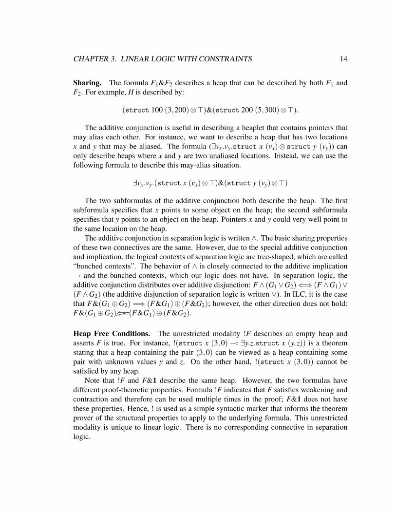
Sharing. The formula F1&F2 describes a heap that can be described by both F1 andF2. For example, H is described by:
(struct 100 (3,200)⊗>)&(struct 200 (5,300)⊗>).
The additive conjunction is useful in describing a heaplet that contains pointers thatmay alias each other. For instance, we want to describe a heap that has two locationsx and y that may be aliased. The formula (∃vx.vy.struct x (vx)⊗ struct y (vy)) canonly describe heaps where x and y are two unaliased locations. Instead, we can use thefollowing formula to describe this may-alias situation.
∃vx.vy.(struct x (vx)⊗>)&(struct y (vy)⊗>)
The two subformulas of the additive conjunction both describe the heap. The firstsubformula specifies that x points to some object on the heap; the second subformulaspecifies that y points to an object on the heap. Pointers x and y could very well point tothe same location on the heap.
The additive conjunction in separation logic is written ∧. The basic sharing propertiesof these two connectives are the same. However, due to the special additive conjunctionand implication, the logical contexts of separation logic are tree-shaped, which are called“bunched contexts”. The behavior of ∧ is closely connected to the additive implication→ and the bunched contexts, which our logic does not have. In separation logic, theadditive conjunction distributes over additive disjunction: F ∧ (G1∨G2)⇐⇒ (F ∧G1)∨(F ∧G2) (the additive disjunction of separation logic is written ∨). In ILC, it is the casethat F&(G1⊕G2) =⇒ (F&G1)⊕ (F&G2); however, the other direction does not hold:F&(G1⊕G2)⇐=(F&G1)⊕ (F&G2).
Heap Free Conditions. The unrestricted modality !F describes an empty heap andasserts F is true. For instance, !(struct x (3,0) ( ∃y.z.struct x (y,z)) is a theoremstating that a heap containing the pair (3,0) can be viewed as a heap containing somepair with unknown values y and z. On the other hand, !(struct x (3,0)) cannot besatisfied by any heap.
Note that !F and F&1 describe the same heap. However, the two formulas havedifferent proof-theoretic properties. Formula !F indicates that F satisfies weakening andcontraction and therefore can be used multiple times in the proof; F&1 does not havethese properties. Hence, ! is used as a simple syntactic marker that informs the theoremprover of the structural properties to apply to the underlying formula. This unrestrictedmodality is unique to linear logic. There is no corresponding connective in separationlogic.
CHAPTER 3. LINEAR LOGIC WITH CONSTRAINTS 15
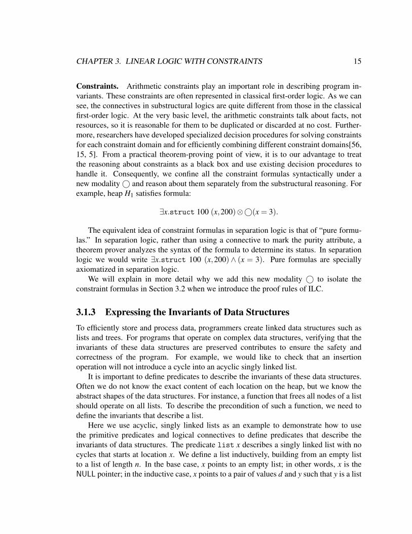
Constraints. Arithmetic constraints play an important role in describing program in-variants. These constraints are often represented in classical first-order logic. As we cansee, the connectives in substructural logics are quite different from those in the classicalfirst-order logic. At the very basic level, the arithmetic constraints talk about facts, notresources, so it is reasonable for them to be duplicated or discarded at no cost. Further-more, researchers have developed specialized decision procedures for solving constraintsfor each constraint domain and for efficiently combining different constraint domains[56,15, 5]. From a practical theorem-proving point of view, it is to our advantage to treatthe reasoning about constraints as a black box and use existing decision procedures tohandle it. Consequently, we confine all the constraint formulas syntactically under anew modality © and reason about them separately from the substructural reasoning. Forexample, heap H1 satisfies formula:
∃x.struct 100 (x,200)⊗©(x = 3).
The equivalent idea of constraint formulas in separation logic is that of “pure formu-las.” In separation logic, rather than using a connective to mark the purity attribute, atheorem prover analyzes the syntax of the formula to determine its status. In separationlogic we would write ∃x.struct 100 (x,200)∧ (x = 3). Pure formulas are speciallyaxiomatized in separation logic.
We will explain in more detail why we add this new modality © to isolate theconstraint formulas in Section 3.2 when we introduce the proof rules of ILC.
3.1.3 Expressing the Invariants of Data StructuresTo efficiently store and process data, programmers create linked data structures such aslists and trees. For programs that operate on complex data structures, verifying that theinvariants of these data structures are preserved contributes to ensure the safety andcorrectness of the program. For example, we would like to check that an insertionoperation will not introduce a cycle into an acyclic singly linked list.
It is important to define predicates to describe the invariants of these data structures.Often we do not know the exact content of each location on the heap, but we know theabstract shapes of the data structures. For instance, a function that frees all nodes of a listshould operate on all lists. To describe the precondition of such a function, we need todefine the invariants that describe a list.
Here we use acyclic, singly linked lists as an example to demonstrate how to usethe primitive predicates and logical connectives to define predicates that describe theinvariants of data structures. The predicate list x describes a singly linked list with nocycles that starts at location x. We define a list inductively, building from an empty listto a list of length n. In the base case, x points to an empty list; in other words, x is theNULL pointer; in the inductive case, x points to a pair of values d and y such that y is a list

CHAPTER 3. LINEAR LOGIC WITH CONSTRAINTS 16
pointer. The formula that describes the base case is ©(x = 0); the formula that describesthe inductive case is ∃d:Si.y:Si.(struct x (d,y)⊗list y). In the second case, the headand the tail of the list are separated by ⊗ to indicate that they are two disjoint pieces ofthe heap. This constraint guarantees the list will be acyclic. The full definition of a list iswritten below, with the two cases connected by the disjunction ⊕.
list x .=©(x = 0)⊕ (∃d∃y.struct x (d,y)⊗list y)
The above definition corresponds to two axioms in ILC:
list x o−© (x = 0)⊕ (∃d∃y.struct x (d,y)⊗list y)
list x−o© (x = 0)⊕ (∃d∃y.struct x (d,y)⊗list y).
The first axiom is strongly reminiscent of definitive clauses in logic programming [73,48]. For the rest of the thesis, we borrow terms and technology from logic programming.Specifically, we call the predicate being defined, the head of the clause; and the formuladefining the predicate, the body of the clause.
The first axiom alone is sufficient to generate the least fixed point semantics for lists.Therefore the definition that we are going to use for list x is given by the followingclause:
list x o−© (x = 0)⊕ (∃d.∃y.struct x (d,y)⊗list y)
We will discuss the consequences of and remedies for omitting the second axiom aspart of the definition in Section 3.4.
A closely related definition, (listseg x y), can be used both to reason about listsand to help us define a more complex data structure, the queue. The definition for(listseg x y) describes an acyclic singly linked list segment starting from location xand ending at y.
listseg x y o−(©(x = y)⊕ (∃d∃z.©¬(x = y)⊗struct x (d,z)⊗listseg z y))
The base case states that (listseg x x) is always true; the second case in the clause bodystates that if x points to a pair of values d and z such that between z and y is a list segment,then between x and y is also a list segment. The inequality of x and y together with thedisjointness of the head and tail of the list segment guarantees noncircularity.
The next example makes use of the listseg predicate to define a queue.
queue x y o−(©(x = 0)⊗©(y = 0))⊕ (∃d.listseg x y⊗struct y (d,0))

CHAPTER 3. LINEAR LOGIC WITH CONSTRAINTS 17
The predicate queue x y describes a queue whose head is x and tail is y. In the clauseabove, the first subformula in the disjunction describes an empty queue where both thehead and tail pointers are NULL pointer. The second subformula of disjunction in thebody describes the situation in which there is at least one element in the queue (pointedto by the tail y). Between the head and the tail of the queue is a list segment. Forexample, the heap H in Figure 3.1 can be viewed as a queue whose head pointer is 100and tail pointer is 300 (e.g.queue 100 300).
Defining tree-shaped data is no more difficult than defining list-shaped data. As anexample, consider the following binary tree definition.
btree x o−© (x = 0)⊕ (∃d∃l∃r.struct x (d, l,r)⊗btree l⊗btree r)
Similar to the list definition, the body of the clause is composed of a disjunction oftwo cases. The base case occurs when x is a NULL pointer. The second case describes atree whose root x points a tuple that contains a left child l and a right child r. Both l andr also point to a binary tree as well.
3.2 Syntax, Semantics, and Proof RulesIn this section, we give the formal definitions of ILC’s syntax, semantics, and proof rules,and give proofs for ILC’s consistency.
3.2.1 SyntaxILC extends intuitionistic linear logic with domain-specific predicates for describing theheap and a new modality © to incorporate constraint formulas into the logic.
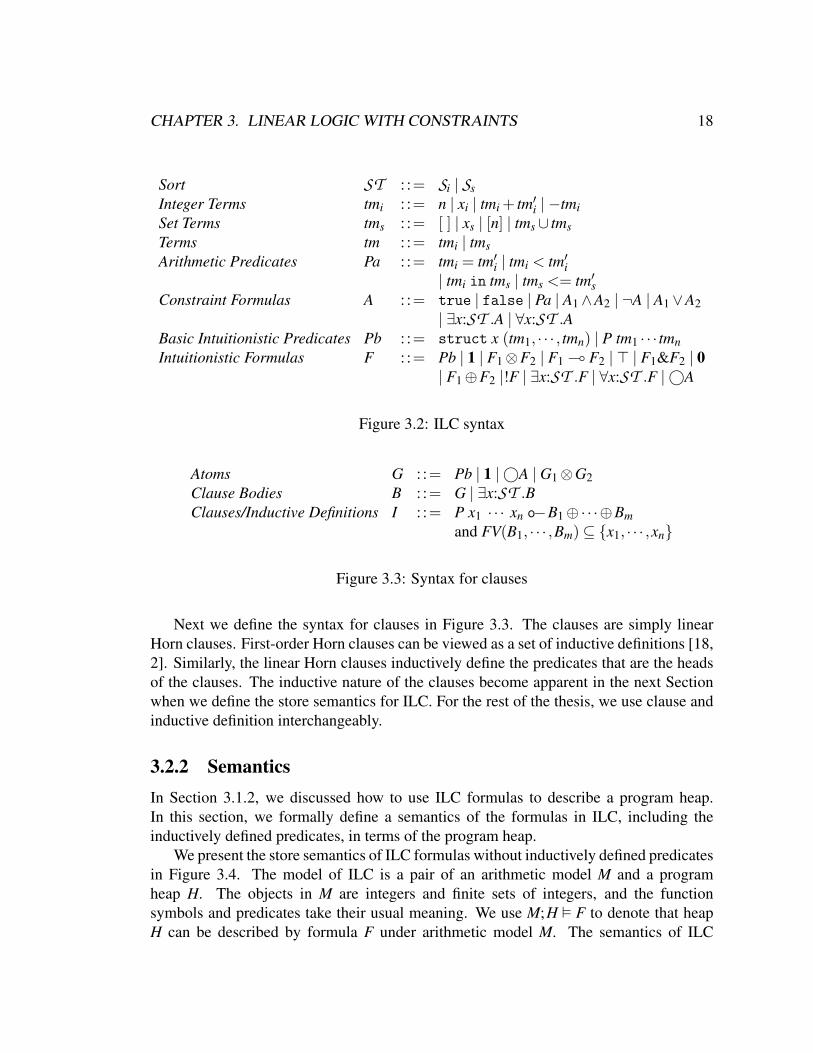
A summary of the syntactic constructs of ILC is shown in Figure 3.2. We use STto range over the sort of terms we consider in this thesis. We use Si to denote integersort and Ss to denote integer set sort. We use tmi to range over integer terms, whichinclude integers, variables, sums and negations of integer terms. We use tms to rangeover set terms. We write [ ] to denote the empty set, [n] to denote a singleton set, andtms ∪ tm′
s denotes the union of two sets. The basic arithmetic predicates, denoted byPa, are equality and the less-than relation on integer terms, set membership, and thesubset relation on sets. The constraint formulas A include basic arithmetic predicates,conjunction, negation, and disjunction of arithmetic formulas. In this thesis, we consideronly Presburger Arithmetic constraints and set constraints. It is straightforward to extendthe syntax of terms and basic arithmetic predicates to include other constraint domains aswell.
ILC formulas F include the basic predicate struct x (tm1, · · · , tmn), inductively de-fined predicates, such as list x, and all of the formulas present in first-order intuitionisticlinear logic. In addition, a new modality © encapsulates constraint formulas.
CHAPTER 3. LINEAR LOGIC WITH CONSTRAINTS 18
Sort ST : := Si | SsInteger Terms tmi : := n | xi | tmi + tm′
i | −tmiSet Terms tms : := [ ] | xs | [n] | tms∪ tmsTerms tm : := tmi | tmsArithmetic Predicates Pa : := tmi = tm′
i | tmi < tm′i
| tmi in tms | tms <= tm′s
Constraint Formulas A : := true | false | Pa | A1∧A2 | ¬A | A1∨A2| ∃x:ST .A | ∀x:ST .A
Basic Intuitionistic Predicates Pb : := struct x (tm1, · · · , tmn) | P tm1 · · · tmnIntuitionistic Formulas F : := Pb | 1 | F1⊗F2 | F1 ( F2 | > | F1&F2 | 0
| F1⊕F2 |!F | ∃x:ST .F | ∀x:ST .F | ©A
Figure 3.2: ILC syntax
Atoms G : := Pb | 1 | ©A | G1⊗G2Clause Bodies B : := G | ∃x:ST .BClauses/Inductive Definitions I : := P x1 · · · xn o−B1⊕·· ·⊕Bm
and FV(B1, · · · ,Bm)⊆ x1, · · · ,xn
Figure 3.3: Syntax for clauses
Next we define the syntax for clauses in Figure 3.3. The clauses are simply linearHorn clauses. First-order Horn clauses can be viewed as a set of inductive definitions [18,2]. Similarly, the linear Horn clauses inductively define the predicates that are the headsof the clauses. The inductive nature of the clauses become apparent in the next Sectionwhen we define the store semantics for ILC. For the rest of the thesis, we use clause andinductive definition interchangeably.
3.2.2 SemanticsIn Section 3.1.2, we discussed how to use ILC formulas to describe a program heap.In this section, we formally define a semantics of the formulas in ILC, including theinductively defined predicates, in terms of the program heap.
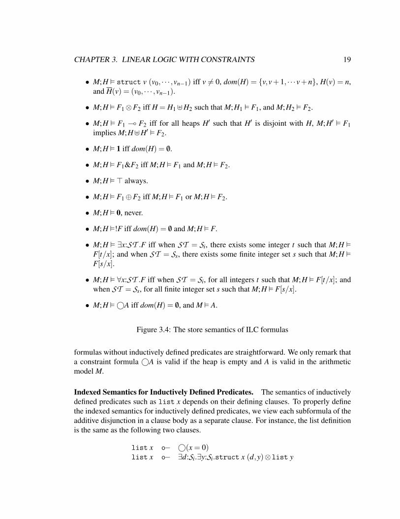
We present the store semantics of ILC formulas without inductively defined predicatesin Figure 3.4. The model of ILC is a pair of an arithmetic model M and a programheap H. The objects in M are integers and finite sets of integers, and the functionsymbols and predicates take their usual meaning. We use M;H F to denote that heapH can be described by formula F under arithmetic model M. The semantics of ILC
CHAPTER 3. LINEAR LOGIC WITH CONSTRAINTS 19
• M;H struct v (v0, · · · ,vn−1) iff v 6= 0, dom(H) = v,v + 1, · · ·v + n, H(v) = n,and H(v) = (v0, · · · ,vn−1).
• M;H F1⊗F2 iff H = H1]H2 such that M;H1 F1, and M;H2 F2.
• M;H F1 ( F2 iff for all heaps H′ such that H′ is disjoint with H, M;H′ F1implies M;H]H′ F2.
• M;H 1 iff dom(H) = /0.
• M;H F1&F2 iff M;H F1 and M;H F2.
• M;H > always.
• M;H F1⊕F2 iff M;H F1 or M;H F2.
• M;H 0, never.
• M;H !F iff dom(H) = /0 and M;H F.
• M;H ∃x:ST .F iff when ST = Si, there exists some integer t such that M;H F[t/x]; and when ST = Ss, there exists some finite integer set s such that M;H F[s/x].
• M;H ∀x:ST .F iff when ST = Si, for all integers t such that M;H F[t/x]; andwhen ST = Ss, for all finite integer set s such that M;H F[s/x].
• M;H ©A iff dom(H) = /0, and M A.
Figure 3.4: The store semantics of ILC formulas
formulas without inductively defined predicates are straightforward. We only remark thata constraint formula ©A is valid if the heap is empty and A is valid in the arithmeticmodel M.
Indexed Semantics for Inductively Defined Predicates. The semantics of inductivelydefined predicates such as list x depends on their defining clauses. To properly definethe indexed semantics for inductively defined predicates, we view each subformula of theadditive disjunction in a clause body as a separate clause. For instance, the list definitionis the same as the following two clauses.
list x o− ©(x = 0)list x o− ∃d:Si.∃y:Si.struct x (d,y)⊗list y

CHAPTER 3. LINEAR LOGIC WITH CONSTRAINTS 20
• M;H P v1 · · ·vm iff ∃n≥ 0 such that M;H n P v1 · · ·vm.
• M;H n P v1 · · ·vm iff exists B ∈ ϒ(P x1 · · ·xm), such that M;H n−1
B[v1, · · ·vm/x1, · · ·xm].
• M;H n struct v (v0, · · · ,vm−1) iff n = 0, v 6= 0, dom(H) = v,v + 1, · · ·v + m,H(v) = m, and H(v) = (v0, · · · ,vm−1).
• M;H n 1 iff n = 0, and dom(H) = /0.
• M;H n ©A iff dom(H) = /0, n = 0, and M A.
• M;H n G1⊗G2 iff H = H1]H2 such that M;H1 n1 G1, M;H2 n2 G2, and n =max(n1,n2).
• M;H n ∃x:ST .G iff When ST = Si, there exists some integer t such that M;H G[t/x]. When ST = Ss, there exists some finite integer set t such that M;H G[s/x].
Figure 3.5: Indexed semantics for inductively defined formulas
Context ϒ contains all the inductive definitions. We write ϒ(P x1 · · ·xn) to denote the setof formulas defining predicate P x1 · · ·xn. For example,
ϒ(list x) = ©(x = 0),(∃d:Si.∃y:Si.struct x (d,y)⊗list y).We use M;H ϒ F to denote that under arithmetic model M, heap H can be describedby formula F, given the inductive definitions in ϒ. Since ϒ is the same throughout thejudgments, we omit it from the judgments.
To properly define the semantics for inductively defined predicates, we use an indexedmodel inspired by the indexed model for recursive types [3]. We use judgment M;H n Fto denote that the model M and the heap H satisfy formula F with index n. Intuitively,the index number indicates the number of applications of the inductive definitions. Forinstance, the judgment M;H n P v1 · · ·vk means that heap H can be described by predicateP v1 · · ·vk by applying the inductive case at most n times starting from the heap describedby the base case. We present the formal definition of the indexed store semantics inFigure 3.5.
When a clause body is composed exclusively of constraint formulas and struct
predicates, the index number of the predicate is 1. This is the base case from whichwe start to build a recursive data structure. For list x,©(x = 0) is the base case. For theinductive case, a recursively defined predicate P with index n describes a heap that can bedescribed by one of P’s clause bodies, B, and the index number of B is n−1. For example,the NULL pointer describes an empty heap with index 1 (M;H 1 list 0). The heaplet H3in Figure 3.1 satisfies list 300 with index 2 (M;H3 2 list 300). The heap (H2]H3)satisfies list 200 with index 3 (M;H2]H3 3 list 200); and H satisfies list 100 with

CHAPTER 3. LINEAR LOGIC WITH CONSTRAINTS 21
index 4 (M;H 4 list 100). Note that the indices are internal representations in definingthe semantics of recursively defined predicates. When describing the program heap forthe purpose of program verification, we often do not and need not to know about theindex number. For instance, the above heaplets are all described by list ` where ` is thestarting location of the list.
3.2.3 Proof RulesThe store semantics specify how we formally model the program heap using logicalformulas. The proof rules define how deductions are carried out in our logic. In reasoningabout the program heap, we first model a heap using logical formulas, then use the proofrules to derive properties of the program heap from those descriptions.
Our logical judgments make use of three logical contexts. The unrestricted contextΓ and the linear context ∆ are the same as in intuitionistic linear logic. The new contextΘ is the unrestricted context for constraint formulas. Contexts Θ and Γ have contraction,weakening, and exchange properties; while ∆ has only exchange.
Unrestricted Constraint Context Θ : := · |Θ,AUnrestricted Context Γ : := · | Γ,FLinear Context ∆ : := · | ∆,F
There are two sequent judgments in our logic.
Θ # Θ′ classical constraint sequent rulesΘ;Γ;∆ =⇒ F intuitionistic linear sequent rules
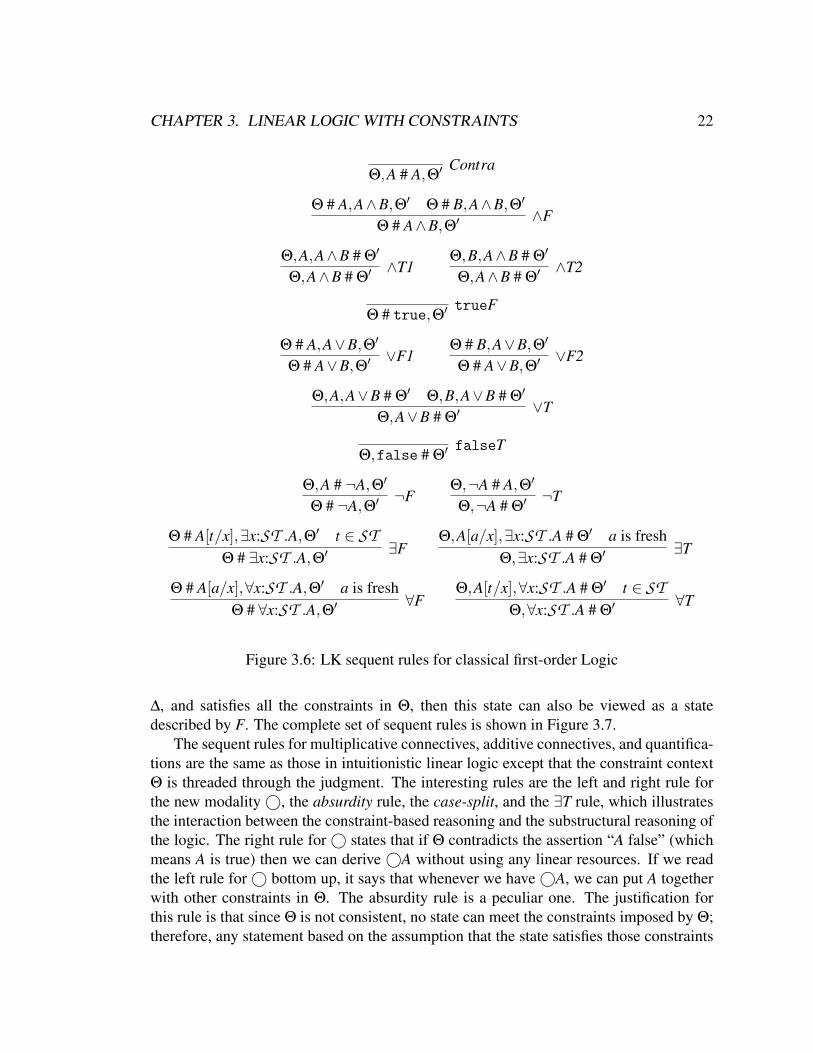
The sequent rules for reasoning about constraints have the form Θ # Θ′, where Θ isthe context for truth assumptions and Θ′ is the context for false assumptions. The sequentΘ # Θ′ can be read as: the truth assumptions in Θ contradict one of the false assumptionsin Θ′. Alternatively, we can say that the conjunction of the formulas in Θ implies thedisjunction of the formulas in Θ′. These sequent rules define first-order classical logicwith equality. The formalization follows Gentzen’s LK formalization [23]. The completeset of rules is shown in Figure 3.6.
To reason about equality between integers, we assume that the Θ context alwayscontains the following axioms about equality.
Aeq1 = ∀x:Si.x = xAeq2 = ∀x:Si.∀y:Si.¬(x = y)∨ ( f (x) = f (y))Aeq3 = ∀x:Si.∀y:Si.¬(x = y)∨¬Pa(x)∨Pa(y)
In Appendix A.1 (Lemma 25 – 28), we show that we can prove reflexivity, symmetry,and transitivity of equality using the above axioms.
The intuitionistic sequent rules have the form Θ;Γ;∆ =⇒ F. An intuitive reading ofthe sequent is that if a state described by unrestricted assumptions in Γ, linear assumptions
CHAPTER 3. LINEAR LOGIC WITH CONSTRAINTS 22
Θ,A # A,Θ′ Contra
Θ # A,A∧B,Θ′ Θ # B,A∧B,Θ′
Θ # A∧B,Θ′ ∧F
Θ,A,A∧B # Θ′
Θ,A∧B # Θ′ ∧T1Θ,B,A∧B # Θ′
Θ,A∧B # Θ′ ∧T2
Θ # true,Θ′ trueF
Θ # A,A∨B,Θ′
Θ # A∨B,Θ′ ∨F1Θ # B,A∨B,Θ′
Θ # A∨B,Θ′ ∨F2
Θ,A,A∨B # Θ′ Θ,B,A∨B # Θ′
Θ,A∨B # Θ′ ∨T
Θ,false # Θ′ falseT
Θ,A # ¬A,Θ′
Θ # ¬A,Θ′ ¬FΘ,¬A # A,Θ′
Θ,¬A # Θ′ ¬T
Θ # A[t/x],∃x:ST .A,Θ′ t ∈ STΘ # ∃x:ST .A,Θ′ ∃F
Θ,A[a/x],∃x:ST .A # Θ′ a is freshΘ,∃x:ST .A # Θ′ ∃T
Θ # A[a/x],∀x:ST .A,Θ′ a is freshΘ # ∀x:ST .A,Θ′ ∀F
Θ,A[t/x],∀x:ST .A # Θ′ t ∈ STΘ,∀x:ST .A # Θ′ ∀T
Figure 3.6: LK sequent rules for classical first-order Logic
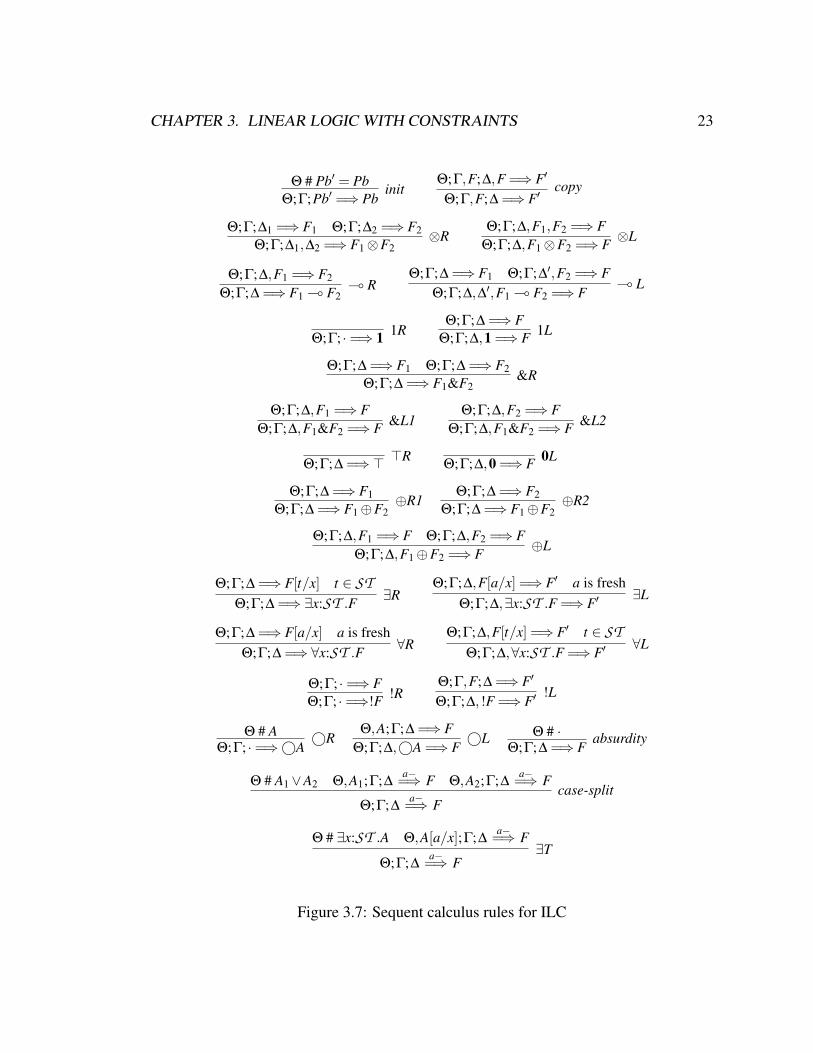
∆, and satisfies all the constraints in Θ, then this state can also be viewed as a statedescribed by F. The complete set of sequent rules is shown in Figure 3.7.
The sequent rules for multiplicative connectives, additive connectives, and quantifica-tions are the same as those in intuitionistic linear logic except that the constraint contextΘ is threaded through the judgment. The interesting rules are the left and right rule forthe new modality ©, the absurdity rule, the case-split, and the ∃T rule, which illustratesthe interaction between the constraint-based reasoning and the substructural reasoning ofthe logic. The right rule for © states that if Θ contradicts the assertion “A false” (whichmeans A is true) then we can derive ©A without using any linear resources. If we readthe left rule for © bottom up, it says that whenever we have ©A, we can put A togetherwith other constraints in Θ. The absurdity rule is a peculiar one. The justification forthis rule is that since Θ is not consistent, no state can meet the constraints imposed by Θ;therefore, any statement based on the assumption that the state satisfies those constraints
CHAPTER 3. LINEAR LOGIC WITH CONSTRAINTS 23
Θ # Pb′ = PbΘ;Γ;Pb′ =⇒ Pb
initΘ;Γ,F;∆,F =⇒ F′
Θ;Γ,F;∆ =⇒ F′copy
Θ;Γ;∆1 =⇒ F1 Θ;Γ;∆2 =⇒ F2Θ;Γ;∆1,∆2 =⇒ F1⊗F2
⊗RΘ;Γ;∆,F1,F2 =⇒ F
Θ;Γ;∆,F1⊗F2 =⇒ F ⊗L
Θ;Γ;∆,F1 =⇒ F2
Θ;Γ;∆ =⇒ F1 ( F2( R
Θ;Γ;∆ =⇒ F1 Θ;Γ;∆′,F2 =⇒ FΘ;Γ;∆,∆′,F1 ( F2 =⇒ F
( L
Θ;Γ; ·=⇒ 1 1RΘ;Γ;∆ =⇒ F
Θ;Γ;∆,1 =⇒ F 1L
Θ;Γ;∆ =⇒ F1 Θ;Γ;∆ =⇒ F2Θ;Γ;∆ =⇒ F1&F2
&R
Θ;Γ;∆,F1 =⇒ FΘ;Γ;∆,F1&F2 =⇒ F &L1
Θ;Γ;∆,F2 =⇒ FΘ;Γ;∆,F1&F2 =⇒ F &L2
Θ;Γ;∆ =⇒> >RΘ;Γ;∆,0 =⇒ F 0L
Θ;Γ;∆ =⇒ F1Θ;Γ;∆ =⇒ F1⊕F2
⊕R1Θ;Γ;∆ =⇒ F2
Θ;Γ;∆ =⇒ F1⊕F2⊕R2
Θ;Γ;∆,F1 =⇒ F Θ;Γ;∆,F2 =⇒ FΘ;Γ;∆,F1⊕F2 =⇒ F ⊕L
Θ;Γ;∆ =⇒ F[t/x] t ∈ STΘ;Γ;∆ =⇒∃x:ST .F ∃R
Θ;Γ;∆,F[a/x] =⇒ F′ a is freshΘ;Γ;∆,∃x:ST .F =⇒ F′
∃L
Θ;Γ;∆ =⇒ F[a/x] a is freshΘ;Γ;∆ =⇒∀x:ST .F ∀R
Θ;Γ;∆,F[t/x] =⇒ F′ t ∈ STΘ;Γ;∆,∀x:ST .F =⇒ F′
∀L
Θ;Γ; ·=⇒ FΘ;Γ; ·=⇒!F !R
Θ;Γ,F;∆ =⇒ F′
Θ;Γ;∆, !F =⇒ F′!L
Θ # AΘ;Γ; ·=⇒©A
©RΘ,A;Γ;∆ =⇒ F
Θ;Γ;∆,©A =⇒ F©L Θ # ·
Θ;Γ;∆ =⇒ Fabsurdity
Θ # A1∨A2 Θ,A1;Γ;∆a−=⇒ F Θ,A2;Γ;∆
a−=⇒ F
Θ;Γ;∆a−=⇒ F
case-split
Θ # ∃x:ST .A Θ,A[a/x];Γ;∆a−=⇒ F
Θ;Γ;∆a−=⇒ F
∃T
Figure 3.7: Sequent calculus rules for ILC

CHAPTER 3. LINEAR LOGIC WITH CONSTRAINTS 24
is simply true. The case-split rule splits a disjunction in the constraint domain. If Θ
entails A1∨A2, then we can split the derivation into two cases: one assumes A1 is true,and the other assumes A2 is true. The ∃T rule makes use of the existentially quantifiedformulas in the constraint domain.
3.2.4 Formal ResultsIn this section we present some of the formal results we have proved about our logic.We have proved cut elimination theorems for our logic, thus proving that our logic isconsistent. By proving the cut elimination theorems, we also established the sub-formulaproperties of our logic: all formulas in a (cut-free) derivation are subformulas of theformulas in the conclusion sequent. We also proved that the proof theory of our logicis sound with regard to its semantics, which means that any theorems we can provesyntactically using the proof rules are valid in the memory model. However, our logic isnot complete with regard to this memory model, which means that there are some validformulas that we cannot prove in the proof system.
Cut Elimination Theorems Cut rules are used to prove the final result via intermediaryresults. We list the four cut rules in our logic below.
Θ,A # Θ′ Θ # A,Θ′
Θ # Θ′Θ # A Θ,A;Γ;∆ =⇒ F
Θ;Γ;∆ =⇒ F
Θ;Γ; ·=⇒ F Θ;Γ,F;∆ =⇒ F′
Θ;Γ;∆ =⇒ F′Θ;Γ;∆ =⇒ F Θ;Γ;∆′,F =⇒ F′
Θ;Γ;∆,∆′ =⇒ F′
The cut elimination theorems state that the cut rules are not necessary in our logic.Given any proof that uses the cut rules, we can always rewrite the proof to not contain anycut rules. The cut elimination theorems consists of four theorems (Theorem 1 through3); one for each cut rule. We use Pfenning’s structural proof technique for cut elimina-tion [62]. We present the theorems and the proof strategy below. The detailed proofs forselected cases can be found in Appendix A.1.
For any valid judgment J, we write D :: J when D is a derivation of J.
Theorem 1 (Law of Excluded Middle)If E :: Θ,A # Θ′ and D :: Θ # A,Θ′ then Θ # Θ′.
Proof (sketch): By induction on the structure of the cut formula A and derivations Dand E . There are four categories of cases: (1) either D or E is the contra rule; (2) the cutformula is the principal formula in the last rule of both D and E ; (3) the cut formula isunchanged in D; and (4) the cut formula is unchanged in E .

CHAPTER 3. LINEAR LOGIC WITH CONSTRAINTS 25
Theorem 2 (Cut Elimination 1)If D :: Θ # A and E :: Θ,A;Γ;∆ =⇒ F then Θ;Γ;∆ =⇒ F
Proof (sketch): By induction on the structure of E . For most cases, the cut formula Ais unchanged in E . We can apply the induction hypothesis on a smaller E . When the lastrule in E is the ©R rule or the absurdity rule, we apply Theorem 1.
Theorem 3 (Cut Elimination 2)1. If D :: Θ;Γ;∆ =⇒ F and E :: Θ;Γ;∆′,F =⇒ F′ then Θ;Γ;∆,∆′ =⇒ F′.
2. If D :: Θ;Γ; ·=⇒ F and E :: Θ;Γ,F;∆ =⇒ F′ then Θ;Γ;∆ =⇒ F′.
Proof (sketch):
1. By induction on the structure of F, and the derivations D and E . There are fourcategories of cases: (1) either D or E is the init rule; (2) the cut formula is theprincipal formula in the last rule of both D and E ; (3) the cut formula is unchangedin D , and (4) the cut formula is unchanged in E . We only apply 2 when the cutformula is strictly smaller.
2. By induction on the structure of D and E . For most cases, the principal cut formulais unchanged in E . When the last rule in E is the copy rule, we apply 1.
We prove the consistency of our logic by demonstrating that we cannot prove false-hood from empty contexts.
Lemma 4We can never derive · # ·.
Proof (sketch): By examining all the proof rules without the cut rule,.
Theorem 5 (Consistency)ILC is consistent.
Proof (sketch): By examining all the proof rules without the cut rule, there is noderivation for judgment: ·; ·; ·=⇒ 0.

CHAPTER 3. LINEAR LOGIC WITH CONSTRAINTS 26
Soundness of Logical Deduction. We also proved the soundness of our proof rulesrelative to our memory model. Because the clauses defining recursive data structuresreside in the context Γ as axioms, there are two parts to the soundness of logical deductiontheorem. One is that the proof rules are sound with regard to the model (Theorem 6); theother is that the axioms defining recursive predicates are sound with regard to the modelas well (Theorem 7).
We use the notationN
∆ to denote the formula obtained by tensoring all the formulasin context ∆ together. We use notation !Γ to denote the context derived from Γ bywrapping the ! modality around each formula in Γ.
The detailed proofs of Theorem 6 and 7 can be found in Appendix A.2.
Theorem 6 (Soundness of Logical Deduction)If Θ;Γ;∆ =⇒ F, σ is a ground substitution for all the free variables in the judgment,M is a model such that M σ(Θ), and M;H σ(
N!Γ⊗
N∆) then M;H σ(F).
Proof (sketch): By induction on the structure of the derivation D :: Θ;Γ;∆ =⇒ F.
Theorem 7 (Soundness of Axioms)For all inductive definitions I such that I ∈ ϒ, M; /0 ϒ I.
Proof (sketch): By examining the semantics of formulas.
3.3 A Sound Decision ProcedureOne of the key steps to developing terminating verification processes based on ILCis to develop a sound and decidable decision procedure for fragments of ILC that areexpressive enough to capture the program invariants that we would like to verify. ILCcontains intuitionistic linear logic as a sublogic, so it is clearly undecidable [47]. In thissection, we identify one fragment of ILC (ILCa−) that has a sound decision procedure,and is expressive enough to reason about invariants of program heaps, including theshape invariants of recursive data structures. This section is organized as follows: InSection 3.3.1, we define ILCa−. In Section 3.3.2 we define a linear residuation calcu-lus, which is sound with regard to ILCa−, and we prove the decidability of the linearresiduation calculus.
3.3.1 ILCa−
ILC combines constraint-based reasoning with linear reasoning; therefore, in the frag-ments of ILC that has sound decision procedures, we need both the constraint-solvingand the linear reasoning to be decidable. There are many decidable first-order theories.

CHAPTER 3. LINEAR LOGIC WITH CONSTRAINTS 27
To illustrate the techniques of our decidability proofs, we only consider Presburger Arith-metic in the constraint domain. It is straightforward to extend the decidability results toinclude other decidable theories at well.
We use the decidability results of linear logic proved by Lincoln et al. [47]. Lincoln etal. proved that intuitionistic linear logic without the unrestricted modality ! is decidable.Lincoln’s technique involved examining the proof rules and noticing that every premiseof each rule is strictly smaller than its consequent (by smaller we mean the numberof connectives in the sequent decreases [47]). Therefore, it is possible to enumerateall derivation trees for a judgment; and consequently, deciding the provability in thisfragment of linear logic can be carried out by checking all possible derivation trees for atleast one valid derivation. We would like to apply this observation to identify a fragmentof ILC that has decidable decision procedures. In ILC, one of the sequent rules whosepremise has more connectives than its consequent is the copy rule:
Θ;Γ,F;∆,F =⇒ F′
Θ;Γ,F;∆ =⇒ F′copy
We rely on the copy rule to move the assumptions from the unrestricted context Γ intothe linear context ∆, where the connectives are decomposed. One important use of thecopy rule is reasoning about recursively defined data structures such as lists. The axiomsfor defining these data structures are unrestricted resources since they do not depend onthe current heap state. These axioms are placed in the unrestricted context Γ. We need touse these axioms many times in a derivation. Each time we make use of the axioms, weapply the copy rule first.
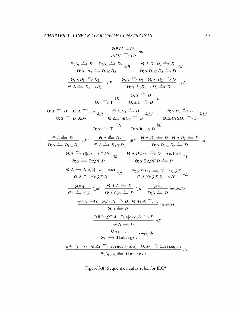
In order to eliminate the copy rule while retaining the ability to reason about recur-sively defined data structures, we add new sequent rules that correspond to the axioms thatdefine those data structures. The resulting logic is ILCa− (a subset of ILC with axioms).The judgment form of ILCa− is Θ;∆
a−=⇒ F. Notice that we completely eliminate the Γ
context, which means that we do not use the ! connective anymore.We use D to denote the formulas that may appear in ILCa−. The formal definition of
D is as follows.
Forms in ILCa− D : := P tm1 · · · tmn | struct x (tm1, · · · , tmn) | 1 | D⊗D′ | D ( D| > | D&D′ | 0 | D⊕D′ | ∃x.D | ∀x.D | ©A
We use the axioms defining listseg as an example to demonstrate how to addsequent rules corresponding to the axioms of the recursively defined predicates in ILCa−.This technique can be extended to other axioms, including the axioms concerning thelist predicate as well.
The following two axioms define the listseg predicate. They are equivalent tothe definitions presented in Section 3.1.3. The free variables in the clause body areuniversally quantified at the outermost level.

CHAPTER 3. LINEAR LOGIC WITH CONSTRAINTS 28
A1 = ∀x.∀y.listseg x y o−© (x = y)A2 = ∀x.∀y.∀d.∀z.listseg x y o−© (¬(x = y))⊗struct x (d,z)⊗listseg z y
The corresponding sequent rules in ILCa− are:
Θ # t = sΘ; · a−=⇒ listseg t s
empty-R
Θ # ¬(t = s) Θ;∆1a−=⇒ struct t (d,u) Θ;∆2
a−=⇒ listseg u s
Θ;∆1,∆2a−=⇒ listseg t s
list
The sequent rule empty-R corresponds to axiom A1 and the rule list corresponds toaxiom A2. In general, the head of the clause becomes the conclusion in the sequent rule,and each of the conjunctive subformulas in the clause body becomes a premise in thesequent rule.
A summary of the sequent rules of ILCa− are in Figure 3.8.We proved the following cut-elimination theorems of ILCa−. The detailed proof is in
Appendix A.3.
Theorem 8 (Cut Elimination 1)If Θ # A and Θ,A;∆
a−=⇒ D then E :: Θ;∆a−=⇒ D
Proof (sketch): By induction on the structure of derivation E .
Theorem 9 (Cut Elimination 2)If Θ;∆
a−=⇒ D and Θ;∆′,D a−=⇒ D′ then Θ;∆,∆′a−=⇒ D′.
We also proved the following soundness and completeness theorems to show thatILCa− is equivalent to ILC with axioms A1 and A2. The details of the proofs are inAppendix A.3
Theorem 10 (Soundness of ILCa−)If Θ;∆
a−=⇒ D then Θ;A1,A2;∆ =⇒ D.
Proof (sketch): By induction on the structure of the derivation Θ;∆a−=⇒ D.
Theorem 11 (Completeness of ILCa−)If Θ;A1,A2;∆ =⇒ D and all the formulas in ∆ are D, then Θ;∆
a−=⇒ D.
Proof (sketch): By induction on the derivation of Θ;A1,A2;∆ =⇒D. Most cases invokethe induction hypothesis directly.
CHAPTER 3. LINEAR LOGIC WITH CONSTRAINTS 29
Θ # Pb′ = Pb
Θ;Pb′ a−=⇒ Pbinit
Θ;∆1a−=⇒ D1 Θ;∆2
a−=⇒ D2
Θ;∆1,∆2a−=⇒ D1⊗D2
⊗RΘ;∆,D1,D2
a−=⇒ D
Θ;∆,D1⊗D2a−=⇒ D
⊗L
Θ;∆,D1a−=⇒ D2
Θ;∆a−=⇒ D1 ( D2
( RΘ;∆
a−=⇒ D1 Θ;∆′,D2a−=⇒ D
Θ;∆,∆′,D1 ( D2a−=⇒ D
( L
Θ; · a−=⇒ 11R
Θ;∆a−=⇒ D
Θ;∆,1 a−=⇒ D1L
Θ;∆a−=⇒ D1 Θ;∆
a−=⇒ D2
Θ;∆a−=⇒ D1&D2
&RΘ;∆,D1
a−=⇒ D
Θ;∆,D1&D2a−=⇒ D
&L1Θ;∆,D2
a−=⇒ D
Θ;∆,D1&D2a−=⇒ D
&L2
Θ;∆a−=⇒ >
>RΘ;∆,0 a−=⇒ D
0L
Θ;∆a−=⇒ D1
Θ;∆a−=⇒ D1⊕D2
⊕R1Θ;∆
a−=⇒ D2
Θ;∆a−=⇒ D1⊕D2
⊕R2Θ;∆,D1
a−=⇒ D Θ;∆,D2a−=⇒ D
Θ;∆,D1⊕D2a−=⇒ D
⊕L
Θ;∆a−=⇒ D[t/x] t ∈ ST
Θ;∆a−=⇒ ∃x:ST .D
∃RΘ;∆,D[a/x] a−=⇒ D′ a is fresh
Θ;∆,∃x:ST .D a−=⇒ D′∃L
Θ;∆a−=⇒ D[a/x] a is fresh
Θ;∆a−=⇒ ∀x:ST .D
∀R Θ;∆,D[t/x] =⇒ D′ t ∈ STΘ;∆,∀x:ST .D =⇒ D′ ∀L
Θ # A
Θ; · a−=⇒ ©A©R
Θ,A;∆a−=⇒ D
Θ;∆,©A a−=⇒ D©L Θ # ·
Θ;∆a−=⇒ D
absurdity
Θ # A1∨A2 Θ,A1;∆a−=⇒ D Θ,A2;∆
a−=⇒ D
Θ;∆a−=⇒ D
case-split
Θ # ∃x:ST .A Θ,A[a/x];∆a−=⇒ D
Θ;∆a−=⇒ D
∃T
Θ # t = s
Θ; · a−=⇒ listseg t sempty-R
Θ # ¬(t = s) Θ;∆1a−=⇒ struct t (d,u) Θ;∆2
a−=⇒ listseg u s
Θ;∆1,∆2a−=⇒ listseg t s
list
Figure 3.8: Sequent calculus rules for ILCa−

CHAPTER 3. LINEAR LOGIC WITH CONSTRAINTS 30
3.3.2 Linear Residuation CalculusIn this section, we define the linear residuation calculus. We prove that the linear residu-ation calculus is sound with regard to ILCa−. We then, prove that the linear residuationcalculus is decidable. Therefore the linear residuation calculus is a sound decision proce-dure for ILCa−
Our linear residuation calculus is inspired by the residuation calculus in Pfenning’slecture notes [63]. Our main reason for developing the linear residuation calculus is toseparate the unification process from the rest of the reasoning. We will explain in moredetail when we explain the sequent rules of the linear residuation calculus.
The judgments of linear residuation calculus have the form: ∆r=⇒ D\R. The for-
mula R is the residuation formula, a first-order formula that capture the unification andarithmetic constraints for deriving D from contexts ∆. This judgment states that ∆ entailsF with the additional constraints R.
The proof rules in the Residuation Calculus is presented in Figure 3.9.The basic idea of the residuation calculus is to accumulate constraints, including
unification constraints and arithmetic constraints, into the residuation formula. For in-stance, in the init rule, we leave checking that P and P′ are the same predicate to theresiduation formula. The validity of the residuation formula requires that Θ implies thatP and P′ are the same. In the ∃R rule, we defer the choice of the term to instantiatethe existential variable. Instead, we substitute x with a fresh variable a, and existentiallyquantify the residuation formula in the premise. Later on we find the witness for theexistentially quantified variable x, when we verify the validity of the residuation formulas.In comparison, in ILCa−’s ∃R rule, the witness for the existentially quantified variable xis guessed by magic. The domain of possible witnesses for x might be infinite and abrute-force method of searching for a witness will not terminate, even though the actualproblem of finding a witness might be decidable. This nonalgorithmic nature of the ∃Rrule makes ILCa− an ill fit to reason about decidability.
There are two parts to derive D from context Θ and ∆. One is to derive judgment∆
r=⇒ D\R; the other is to prove that Θ entails the residuation formula R.
Soundness We proved that the residuation calculus is sound with regard to ILCa−. Theproofs can be found in Appendix A.4. The soundness theorem (Theorem 12) states thatif we can derive D with a residuation formula R, and prove that Θ entails R, then we canderive F in ILCa−.
Theorem 12 (Soundness of Residuation Caclulus)If D :: ∆
r=⇒ D\R then given any Θ such that Θ # R, then Θ;∆a−=⇒ D.
Proof (sketch): By induction on the structure of derivation D .

CHAPTER 3. LINEAR LOGIC WITH CONSTRAINTS 31
Pb r=⇒ Pb′\Pb .= Pb′init
∆1r=⇒ D1\R1 ∆2
r=⇒ D2\R2
∆1,∆2r=⇒ D1⊗D2\R1∧R2
⊗R∆,D1,D2
r=⇒ D\R
∆,D1⊗D2r=⇒ D\R
⊗L
∆,D1r=⇒ D2\R
∆r=⇒ D1 ( D2\R
( R∆
r=⇒ D1\R1 ∆′,D2r=⇒ D\R2
∆,∆′,D1 ( D2r=⇒ D\R1∧R2
( L
· r=⇒ 1\true1R
∆r=⇒ D\R
∆,1 r=⇒ D\R1L
∆r=⇒ D1\R1 ∆
r=⇒ D2\R2
∆r=⇒ D1&D2\R1∧R2
&R∆,D1
r=⇒ D\R
∆,D1&D2r=⇒ D\R
&L1∆,D2
r=⇒ D\R
∆,D1&D2r=⇒ D\R
&L2
∆r=⇒ >\true
>R∆,0 r=⇒ D\true
0L
∆r=⇒ D1\R
∆r=⇒ D1⊕D2\R
⊕R1∆
r=⇒ D2\R
∆r=⇒ D1⊕D2\R
⊕R2∆,D1
r=⇒ D\R1 ∆,D2r=⇒ D\R2
∆,D1⊕D2r=⇒ D\R1∧R2
⊕L
∆r=⇒ D[a/x]\R[a/x] a is fresh
∆r=⇒ ∃x.D\∃x.R
∃R∆,D[a/x] r=⇒ D′\R[a/x] a is fresh
∆,∃x.D r=⇒ D′\∀x.R∃L
∆r=⇒ D[a/x]\R[a/x] a is fresh
∆r=⇒ ∀x.D\∀x.R
∀R∆,D[a/x] r=⇒ D′\R[a/x] a is fresh
∆,∀x.D r=⇒ D′\∃x.R∀L
· r=⇒ ©A\A©R
∆r=⇒ D\R
∆,©A r=⇒ D\¬A∨R©L
∆r=⇒ D\false
absurdity
· r=⇒ listseg t s\ t = sempty-R
∆1r=⇒ struct t (d,next)\R1 R1 6= false ∆2
r=⇒ listseg next s\R2
∆1,∆2r=⇒ listseg t s\R1∧R2∧¬(t = s)
list
Figure 3.9: Linear residuation calculus
Decidability. To prove that the linear residuation calculus is decidable, we have toprove that building a residuation derivation is decidable and that checking the validityof the residuation formulas is also decidable.

CHAPTER 3. LINEAR LOGIC WITH CONSTRAINTS 32
Checking the validity of residuation formulas is a decidable process, because theresiduation formulas are Presburger Arithmetic formulas the validity of which is provento be decidable.
Lemma 13Θ # R is decidable.
Proof (sketch): Presburger Arithmetic is decidable.
Once we know the residual formulas are valid, we are left to prove that the residuationcalculus is decidable. As we mentioned earlier, if we are able to argue that every premiseof each rule in the residuation calculus is strictly smaller than its consequent, then wecan prove the decidability of the residuation calculus. By examining all the rules inresiduation calculus, the only rule whose premises are not obviously smaller than itsconsequent is the following list rule.
D1 :: ∆1r=⇒ struct t (d,next)\R1 R1 6= false D2 :: ∆2
r=⇒ listseg next s\R2
∆1,∆2r=⇒ listseg t s\R1∧R2∧¬(t = s)
list
First we impose an ordering of predicates: the “struct” predicate is smaller than theuser-defined predicates. This makes the derivation D1 smaller than the conclusion. Next,we prove that the side condition: R1 6= false makes ∆1 to be nonempty (the proof isdone by examining all the rules in the residuation calculus). As a result, derivation D2contains less connectives than the conclusion.
Lemma 14The residuation calculus is decidable.
Proof (sketch): By examination of the proof rules. The premise of each rule is strictlysmaller than its conclusion, so there is finite number of possible proof trees (a similarproof technique was made in Lincoln’s paper on the decidability properties of proposi-tional linear logic [47]).
3.4 Additional AxiomsWe mentioned in Section 3.1.3 that the semantic definition of a data structures has boththe if and only if directions: x is a list if and only if x is a null pointer or x points to apair of values d and next, such that next points to a list. However, we only use the ifdirection as the defining clause of a list. The memory model contains axioms such as(list 0 ( 1), which are currently not derivable from the proof rules. We can overcomethis incompleteness by adding more axioms about data structures to the proof system.

CHAPTER 3. LINEAR LOGIC WITH CONSTRAINTS 33
In this section, we add more proof rules to strengthen the proof system. There aretwo categories of these additional rules: one, to deal with list shapes; the other, to extractinequality from separation. We have proved that these proof rules are sound with regardto the memory model.
3.4.1 More Axioms About ShapesAs we mentioned before, the proof rules empty-R and list are not strong enough to provecertain properties of list shapes. For instance, we cannot prove that two list segmentslistseg t s and listseg s w can be combined to one list segment listseg t w. To dothis, we need to add more rules into the proof system. We list the additional rules below:
Θ # t = s Θ;∆a−=⇒ D
Θ;∆,listseg t s a−=⇒ Dempty-L
Θ # ¬(t = s) Θ;∆,listseg t s a−=⇒ D
Θ;∆,struct t (d,w),listseg w s a−=⇒ Dlist-1
Θ # ¬(t = s) Θ;∆,struct s (v1,v2),listseg t s a−=⇒ D
Θ;∆,struct s (v1,v2),listseg t w,listseg w s a−=⇒ Dlist-2
Θ # ¬(t = s) Θ # ¬(s = u) Θ;∆,listseg s u,listseg t s a−=⇒ D
Θ;∆,listseg s u,listseg t w,listseg w s a−=⇒ Dlist-3
Θ # s = 0 Θ;∆,listseg t s a−=⇒ D
Θ;∆,listseg t w,listseg w s a−=⇒ Dlist-4
Rule Empty-L acknowledges that listseg t t is an empty heap, and therefore canbe removed from the linear context. Rule list-1 is similar to the list rule, except thatlist-1 rule applies directly to the linear context. The last three rules state that we canfold two connecting list segments, listseg t w and listseg w s, into one list segment,listseg t s. However, since we require list segments to be acyclic, we need to ensure thatthe end of the second list segment y does not point into the first segment, listseg t w.The last three rules use three different side conditions to ensure the acyclic property.Rules list-2 and list-3 use the semantics of separation. The basic idea is that if s is anallocated location and disjoint from list segment listseg t w, then s cannot possiblypoint into list segment listseg t w. In the list-2 rule, the witness is the predicatestruct s (v1,v2). In the list-3 rule, the evidence is that y points to a nonempty list. In thelast rule, list-4, y is NULL pointer; therefore, s cannot point into the first list segment.
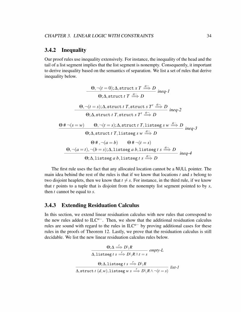
CHAPTER 3. LINEAR LOGIC WITH CONSTRAINTS 34
3.4.2 InequalityOur proof rules use inequality extensively. For instance, the inequality of the head and thetail of a list segment implies that the list segment is nonempty. Consequently, it importantto derive inequality based on the semantics of separation. We list a set of rules that deriveinequality below.
Θ,¬(t = 0);∆,struct x T a−=⇒ D
Θ;∆,struct t T a−=⇒ Dineq-1
Θ,¬(t = s);∆,struct t T,struct s T ′ a−=⇒ D
Θ;∆,struct t T,struct s T ′ a−=⇒ Dineq-2
Θ # ¬(s = w) Θ,¬(t = s);∆,struct t T,listseg s w a−=⇒ D
Θ;∆,struct t T,listseg s w a−=⇒ Dineq-3
Θ # ,¬(a = b) Θ # ¬(t = s)Θ,¬(a = t),¬(b = s);∆,listseg a b,listseg t s a−=⇒ D
Θ;∆,listseg a b,listseg t s a−=⇒ Dineq-4
The first rule uses the fact that any allocated location cannot be a NULL pointer. Themain idea behind the rest of the rules is that if we know that locations t and s belong totwo disjoint heaplets, then we know that t 6= s. For instance, in the third rule, if we knowthat t points to a tuple that is disjoint from the nonempty list segment pointed to by s,then t cannot be equal to s.
3.4.3 Extending Residuation CalculusIn this section, we extend linear residuation calculus with new rules that correspond tothe new rules added to ILCa−. Then, we show that the additional residuation calculusrules are sound with regard to the rules in ILCa− by proving additional cases for theserules in the proofs of Theorem 12. Lastly, we prove that the residuation calculus is stilldecidable. We list the new linear residuation calculus rules below.
Θ;∆r=⇒ D\R
∆,listseg t s r=⇒ D\R∧ t = sempty-L
Θ;∆,listseg t s r=⇒ D\R
∆,struct t (d,w),listseg w s r=⇒ D\R∧¬(t = s)list-1

CHAPTER 3. LINEAR LOGIC WITH CONSTRAINTS 35
Θ;∆,struct s (v1,v2),listseg t s r=⇒ D\R
∆,struct s (v1,v2),listseg t w,listseg w s r=⇒ D\R∧¬(t = s)list-2
∆,listseg s u,listseg t s r=⇒ D\R
∆,listseg s u,listseg t w,listseg w s r=⇒ D\R∧ (¬(t = s)∧¬(s = u))list-3
∆,struct x T r=⇒ D\R
∆,struct t T r=⇒ D\(t = 0)∨Rineq-1
Θ,¬(t = s);∆,struct t T,struct s T ′ r=⇒ D\R
∆,struct t T,struct s T ′ r=⇒ D\(t = s)∨Rineq-2
∆,struct t T,listseg s w r=⇒ D\R
∆,struct t T,listseg s w r=⇒ D\¬(s = w)∧ ((t = w)∨R)ineq-3
∆,listseg a b,listseg t s r=⇒ D\R
∆,listseg a b,listseg t s r=⇒ D\¬(a = b)∧¬(t = s)∧ ((a = t)∨ (b = s)∨R)ineq-4
We proved that with these additional rules, the linear residuation calculus is sound withregard to ILCa− with additional rules.
We need to show that the validity of the residuation formulas is decidable and thelinear residuation calculus is decidable. The additional rules do not change the syntaxof residuation formulas, so the validity of residuation formulas is still decidable. Therules concerning lists clearly obey the constraint that the premises are smaller than theconclusion, therefore the linear residuation calculus is still decidable with the inclusionof these rules. However, the premise of the rules dealing with inequality has the samelinear context as its consequent. To obtain a decidable decision procedure, we developeda sound algorithm that only applies the rules ineq-1 to ineq-4 a finite number of times.Algorithm A
From the goal sequence, we apply rules ineq-1 to ineq-4 until no more inequality canbe derived that is not in R. We only apply rules ineq-1 to ineq-4 after each left rule, untilno more inequality can be derived.
Theorem 15 (Termination of Algorithm A)By using Algorithm A, we either find the valid derivation and terminate with success orexhaust all possible derivations and terminate with failure.
Proof (sketch): The premises of the proof rules other than inequality are smaller thantheir conclusions, and the inequality rules are only applied finite number of times; there-fore, it is possible to enumerate all derivation trees. A saturation point for inequality rulescan be reached because there is a finite number of inequalities that can be derived.
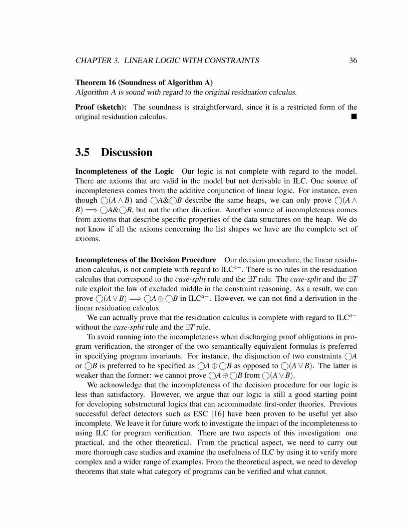
CHAPTER 3. LINEAR LOGIC WITH CONSTRAINTS 36
Theorem 16 (Soundness of Algorithm A)Algorithm A is sound with regard to the original residuation calculus.
Proof (sketch): The soundness is straightforward, since it is a restricted form of theoriginal residuation calculus.
3.5 DiscussionIncompleteness of the Logic Our logic is not complete with regard to the model.There are axioms that are valid in the model but not derivable in ILC. One source ofincompleteness comes from the additive conjunction of linear logic. For instance, eventhough ©(A∧ B) and ©A&©B describe the same heaps, we can only prove ©(A∧B) =⇒©A&©B, but not the other direction. Another source of incompleteness comesfrom axioms that describe specific properties of the data structures on the heap. We donot know if all the axioms concerning the list shapes we have are the complete set ofaxioms.
Incompleteness of the Decision Procedure Our decision procedure, the linear residu-ation calculus, is not complete with regard to ILCa−. There is no rules in the residuationcalculus that correspond to the case-split rule and the ∃T rule. The case-split and the ∃Trule exploit the law of excluded middle in the constraint reasoning. As a result, we canprove ©(A∨B) =⇒©A⊕©B in ILCa−. However, we can not find a derivation in thelinear residuation calculus.
We can actually prove that the residuation calculus is complete with regard to ILCa−
without the case-split rule and the ∃T rule.To avoid running into the incompleteness when discharging proof obligations in pro-
gram verification, the stronger of the two semantically equivalent formulas is preferredin specifying program invariants. For instance, the disjunction of two constraints ©Aor ©B is preferred to be specified as ©A⊕©B as opposed to ©(A∨B). The latter isweaker than the former: we cannot prove ©A⊕©B from ©(A∨B).
We acknowledge that the incompleteness of the decision procedure for our logic isless than satisfactory. However, we argue that our logic is still a good starting pointfor developing substructural logics that can accommodate first-order theories. Previoussuccessful defect detectors such as ESC [16] have been proven to be useful yet alsoincomplete. We leave it for future work to investigate the impact of the incompleteness tousing ILC for program verification. There are two aspects of this investigation: onepractical, and the other theoretical. From the practical aspect, we need to carry outmore thorough case studies and examine the usefulness of ILC by using it to verify morecomplex and a wider range of examples. From the theoretical aspect, we need to developtheorems that state what category of programs can be verified and what cannot.

Chapter 4
Static Verification Using ILC
In this chapter, we demonstrate how to verify programs with pointer operations usingour logic. We define a simple imperative language that includes all the essential pointeroperations such as allocation, deallocation, dereference and updates. This language alsoallow programmers to define recursive data structures such as lists and trees. We thendefine verification generation rules for statements in this language. Given a statement inthis imperative language and a postcondition the verification generation rule can generatea verification condition (VC) that describes the required heap state before evaluating thisstatement so that the statement is memory safe and that the postcondition holds afterthe evaluation of the statement. The goal of the static verification system is to verifythat a program conforms with its specified pre- and post-conditions using the verificationcondition generation rules. In the end, we provide proofs that the verification conditiongeneration rules are sound with regard to the operational semantics of the programs.
4.1 SyntaxThe simple imperative language we are defining here includes control flow, functions,mutable references, and recursive data structures. The syntactic constructs of our lan-guage are shown in Figure 4.1.
In this language, the syntax for formulas has a few minor changes from those pre-sented in the previous chapter: we write “,” in place of ⊗, and “;” in place of ⊕; wewrite xF to denote ∀x.F, and [x]F to denote ∃x.F. For example, the list definition inSection 3.1.3 is now written as:
list x o− O(x = 0); (struct x (d,y), list y)
However, we still use the notation from Chapter 3 to present the rules and examples inthis chapter, so that they are easily readable. The programmers write in the syntax shownin Figure 4.1.
37
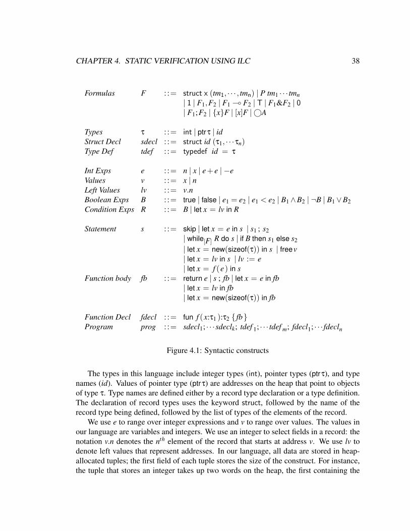
CHAPTER 4. STATIC VERIFICATION USING ILC 38
Formulas F : := struct x (tm1, · · · , tmn) | P tm1 · · · tmn| 1 | F1,F2 | F1 ( F2 | T | F1&F2 | 0| F1;F2 | xF | [x]F | ©A
Types τ : := int | ptrτ | idStruct Decl sdecl : := struct id (τ1, · · ·τn)Type Def tdef : := typedef id = τ
Int Exps e : := n | x | e+ e | −eValues v : := x | nLeft Values lv : := v.nBoolean Exps B : := true | false | e1 = e2 | e1 < e2 | B1∧B2 | ¬B | B1∨B2Condition Exps R : := B | let x = lv in R
Statement s : := skip | let x = e in s | s1 ; s2| while[F] R do s | if B then s1 else s2
| let x = new(sizeof(τ)) in s | freev| let x = lv in s | lv := e| let x = f (e) in s
Function body fb : := return e | s ; fb | let x = e in fb| let x = lv in fb| let x = new(sizeof(τ)) in fb
Function Decl fdecl : := fun f (x:τ1 ):τ2 fbProgram prog : := sdecl1; · · ·sdeclk; tdef 1; · · · tdef m; fdecl1; · · · fdecln
Figure 4.1: Syntactic constructs
The types in this language include integer types (int), pointer types (ptrτ), and typenames (id). Values of pointer type (ptrτ) are addresses on the heap that point to objectsof type τ. Type names are defined either by a record type declaration or a type definition.The declaration of record types uses the keyword struct, followed by the name of therecord type being defined, followed by the list of types of the elements of the record.
We use e to range over integer expressions and v to range over values. The values inour language are variables and integers. We use an integer to select fields in a record: thenotation v.n denotes the nth element of the record that starts at address v. We use lv todenote left values that represent addresses. In our language, all data are stored in heap-allocated tuples; the first field of each tuple stores the size of the construct. For instance,the tuple that stores an integer takes up two words on the heap, the first containing the

CHAPTER 4. STATIC VERIFICATION USING ILC 39
Instructions ι : := s | fbEvaluation Context C : := [ ] | [ ] ; ι
Control Stack K : := · | C [(let x = [ ] in s )].K
Code Context Ψ : := · |Ψ, f 7→ (a:τa ):τ f fb [E]Pre∀ret.PostType Context T : := · | T,τ 7→ τ′ | τ 7→ (τ1, · · ·τn)
Figure 4.2: Runtime syntactic constructs
size of the integer which is 1, the second containing the integer. Assuming the startingaddress of the tuple is v, the left value for accessing this integer is v.1. We use B to rangeover boolean expressions. We use R to denote the conditional expression in while loops.We will explain the use of R when we explain while loops.
The statements include skip, variable binding, sequencing, while loops, if branching,allocation, deallocation, dereference, and assignment.
A while loop while[F] R do s is annotated with loop invariant F. The conditionalexpression R evaluates to a boolean that determines whether to exit or to re-enter the loop.The variables in the loop body of the while loop are bound by the let expression in thecondition R. For example, in the statement (while[>] let x = y.1 in x > 0 do y.1 := x−1),the variable x in the loop body is bound by the let expression. The special structure andscoping rules for condition expressions simplify the verification condition generation.
We use sizeof(τ) to denote the size of an object of type τ. The allocation statementuses the keyword new to allocate a tuple for an object of type τ.
We write fb to denote function bodies, which always end with a return statement.A program contains record type declarations, type definitions, and a list of functiondeclarations. The entry point of the program is the main function.
In order to generate verification conditions properly from statements, we requirethe statements be in A-Normal form. Naturally, an implementation would allow pro-grammers to write ordinary expressions and then unwind them to A-Normal form forverification.
4.2 Operational SemanticsWe list all the run-time constructs needed in defining the operational semantics in Fig-ure 4.2. We write ι to denote either a statement or a function body. We use an evaluationcontext C to specify the left-to-right execution order. We also make use of a control stackK to keep track of function calling order. A control stack is a list of evaluation contextswaiting for the return of a function call. A code context Ψ maps function names to theirdefinitions and their pre- and post- conditions. For the core language, we assume all
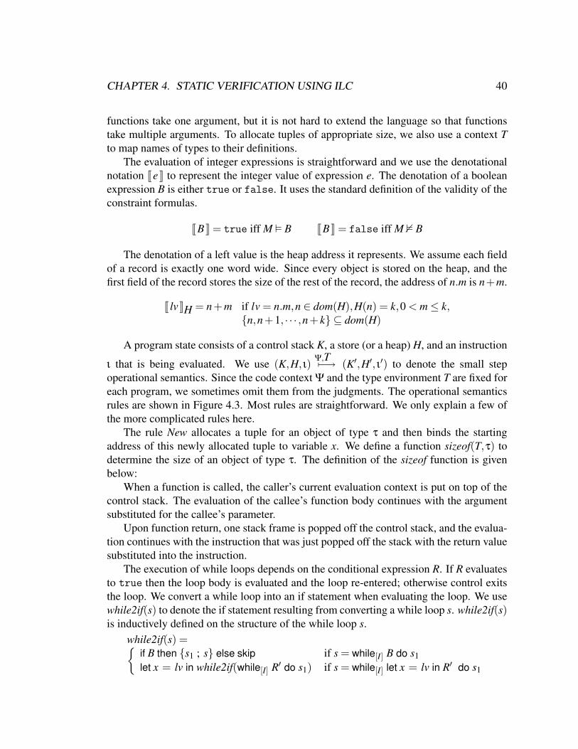
CHAPTER 4. STATIC VERIFICATION USING ILC 40
functions take one argument, but it is not hard to extend the language so that functionstake multiple arguments. To allocate tuples of appropriate size, we also use a context Tto map names of types to their definitions.
The evaluation of integer expressions is straightforward and we use the denotationalnotation JeK to represent the integer value of expression e. The denotation of a booleanexpression B is either true or false. It uses the standard definition of the validity of theconstraint formulas.
JBK = true iff M B JBK = false iff M 2 B
The denotation of a left value is the heap address it represents. We assume each fieldof a record is exactly one word wide. Since every object is stored on the heap, and thefirst field of the record stores the size of the rest of the record, the address of n.m is n+m.
J lvKH = n+m if lv = n.m,n ∈ dom(H),H(n) = k,0 < m≤ k,n,n+1, · · · ,n+ k ⊆ dom(H)
A program state consists of a control stack K, a store (or a heap) H, and an instruction
ι that is being evaluated. We use (K,H, ι)Ψ,T7−→ (K′,H′, ι′) to denote the small step
operational semantics. Since the code context Ψ and the type environment T are fixed foreach program, we sometimes omit them from the judgments. The operational semanticsrules are shown in Figure 4.3. Most rules are straightforward. We only explain a few ofthe more complicated rules here.
The rule New allocates a tuple for an object of type τ and then binds the startingaddress of this newly allocated tuple to variable x. We define a function sizeof(T,τ) todetermine the size of an object of type τ. The definition of the sizeof function is givenbelow:
When a function is called, the caller’s current evaluation context is put on top of thecontrol stack. The evaluation of the callee’s function body continues with the argumentsubstituted for the callee’s parameter.
Upon function return, one stack frame is popped off the control stack, and the evalua-tion continues with the instruction that was just popped off the stack with the return valuesubstituted into the instruction.
The execution of while loops depends on the conditional expression R. If R evaluatesto true then the loop body is evaluated and the loop re-entered; otherwise control exitsthe loop. We convert a while loop into an if statement when evaluating the loop. We usewhile2if(s) to denote the if statement resulting from converting a while loop s. while2if(s)is inductively defined on the structure of the while loop s.
while2if(s) =if B then s1 ; s else skip if s = while[I] B do s1let x = lv in while2if(while[I] R′ do s1) if s = while[I] let x = lv in R′ do s1
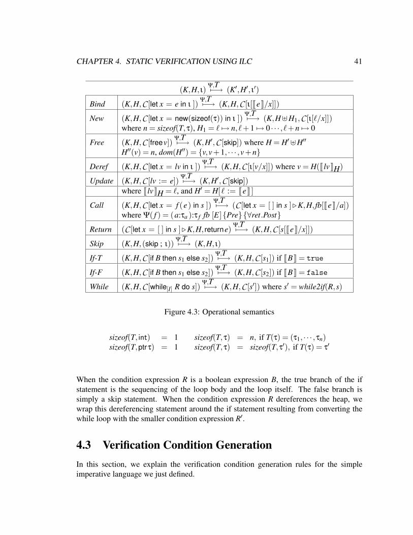
CHAPTER 4. STATIC VERIFICATION USING ILC 41
(K,H, ι)Ψ,T7−→ (K′,H′, ι′)
Bind (K,H,C [let x = e in ι ])Ψ,T7−→ (K,H,C [ι[JeK/x]])
New (K,H,C [let x = new(sizeof(τ)) in ι ])Ψ,T7−→ (K,H]H1,C [ι[`/x]])
where n = sizeof(T,τ), H1 = ` 7→ n, `+1 7→ 0 · · · , `+n 7→ 0
Free (K,H,C [freev])Ψ,T7−→ (K,H′,C [skip]) where H = H′]H′′
H′′(v) = n, dom(H′′) = v,v+1, · · · ,v+n
Deref (K,H,C [let x = lv in ι ])Ψ,T7−→ (K,H,C [ι[v/x]]) where v = H(J lvKH)
Update (K,H,C [lv := e])Ψ,T7−→ (K,H′,C [skip])
where J lvKH = `, and H′ = H[` := JeK ]
Call (K,H,C [let x = f (e) in s ])Ψ,T7−→ (C [let x = [ ] in s ].K,H, fb[JeK/a])
where Ψ( f ) = (a:τa ):τ f fb [E]Pre∀ret.Post
Return (C [let x = [ ] in s ].K,H, returne)Ψ,T7−→ (K,H,C [s[JeK/x]])
Skip (K,H,(skip ; ι))Ψ,T7−→ (K,H, ι)
If-T (K,H,C [if B then s1 else s2])Ψ,T7−→ (K,H,C [s1]) if JBK = true
If-F (K,H,C [if B then s1 else s2])Ψ,T7−→ (K,H,C [s2]) if JBK = false
While (K,H,C [while[I] R do s])Ψ,T7−→ (K,H,C [s′]) where s′ = while2if(R,s)
Figure 4.3: Operational semantics
sizeof(T, int) = 1 sizeof(T,τ) = n, if T(τ) = (τ1, · · · ,τn)sizeof(T,ptrτ) = 1 sizeof(T,τ) = sizeof(T,τ′), if T(τ) = τ′
When the condition expression R is a boolean expression B, the true branch of the ifstatement is the sequencing of the loop body and the loop itself. The false branch issimply a skip statement. When the condition expression R dereferences the heap, wewrap this dereferencing statement around the if statement resulting from converting thewhile loop with the smaller condition expression R′.
4.3 Verification Condition GenerationIn this section, we explain the verification condition generation rules for the simpleimperative language we just defined.

CHAPTER 4. STATIC VERIFICATION USING ILC 42
4.3.1 System SetupEach function in the program has be to annotated with its pre- and post-condition, andloops are annotated with loop invariants. The precondition describes the required pro-gram state before entering the function, and the postcondition describes the requiredprogram state after executing the function body.
The verification generation happens at compile time. There are two ways to verify ifthe program satisfies the specified pre- and post-conditions. One is forward reasoning,we symbolically execute the function body against the precondition. We then examineif the specified postcondition is satisfied at the end of the execution by proving thatthe formula resulting from the symbolic execution logically entails the post-condition.The other method is backward reasoning, we generate a verification condition (VC) byanalyzing the program backward from the postcondition. The VC has the property that ifthe initial program states satisfy the VC, then the program will execute safely and if theprogram terminates then the ending state will satisfy the specified postcondition. Sincewe assume that the precondition holds before the execution of the function, the next stepis to examine if the verification condition is logically entailed by the precondition.
The technique we present in this section is a backward reasoning technique. The mainjudgment for verification condition generation has the following form.
E `Ψ,T P ι Q.
P ι Q is a Hoare triple where P is the precondition and Q is the postcondition. Thecontext E maps variables to their types.
The verification condition generation rules for dereferencing and updating recursivelydefined data structures depend on the invariants of individual data structures. To demon-strate how the system works, we take acyclic singly linked lists as an example. Thesystem can be extended in a similar way to deal with other recursively defined datastructures as well.
We assume the programs contain the following type definitions for lists, which ismuch like that in C: each list node has a data field and a field containing the pointer toanother list node.
struct node (int; ptr(node))typedef list= ptr(node)
Auxiliary Notations. Most verification condition generation rules use the variable typ-ing context E to determine the size of the tuple allocated for the variables in the domainof E. Below is the BNF definition of E.
Typing Context E : := · | E,x : τ

CHAPTER 4. STATIC VERIFICATION USING ILC 43
The judgment E `T x : τ denotes that variable x has type τ according to context E,and the type definitions in T. Judgment T ` τ = τ′ means that τ and τ′ are equivalent giventhe list of type definitions in T. We show the main judgments below.
E `T x : τ T ` τ = τ′
E `T x : τ′
T(τ′) = τ
T ` τ = τ′T ` τ = τ′ T ` τ′ = τ′′
T ` τ = τ′′
We use T(τ,n) to denote the type of the nth field of record type τ.For the rest of this section, we explain the key verification generation rules. A
summary of all the verification condition generation rules can be found in Appendix B.Most of the rules that deal with simple allocation, deallocation, dereference, and updatesare identical to O’Hearn’s weakest precondition generation [35] except that ∗ is replacedby ⊗, −∗ by ( and ∧ by &, and proper placement of the © modality. What is new inour systems is that we also include rules for while loops, function calls, and statementsthat operate on recursively defined data structures.
4.3.2 Verification Condition Generation RulesAllocation. In generating verification condition for the allocation statement, we firstdecide the size of the tuple to be allocated using the sizeof function. Next, we generate theverification condition (P) for instruction ι. The precondition for the allocation statementuses linear implication ( to describe a program heap waiting for a tuple to be allocated.The forall quantifier over the starting address of the newly allocated tuple guarantees thefreshness of the variable, which in turn ensures that y denotes a location that is not yetallocated.
sizeof(T,τ) = n E,x:ptrτ ` P ι Q x /∈ FV(Q)E ` ∀y.struct y (0, · · · ,0) ( P[y/x]
let x = new(sizeof(τ)) in ι
Q
new
Deallocation. The verification condition for the deallocation statement asserts that xindeed is allocated on the heap (∃x1 · ∃xn.struct x (x1, · · · ,xn)). The multiplicativeconjunction ⊗ is crucial here, since it makes sure that the tuple to be freed is separatefrom the rest of the heap. As a result, location x cannot be accessed again after it is freed,which eliminates the error of double freeing.
E ` x : ptr(τ) sizeof(T,τ) = nE ` ∃x1. · · ·∃xn.struct x (x1, · · · ,xn)⊗Q freex Q free
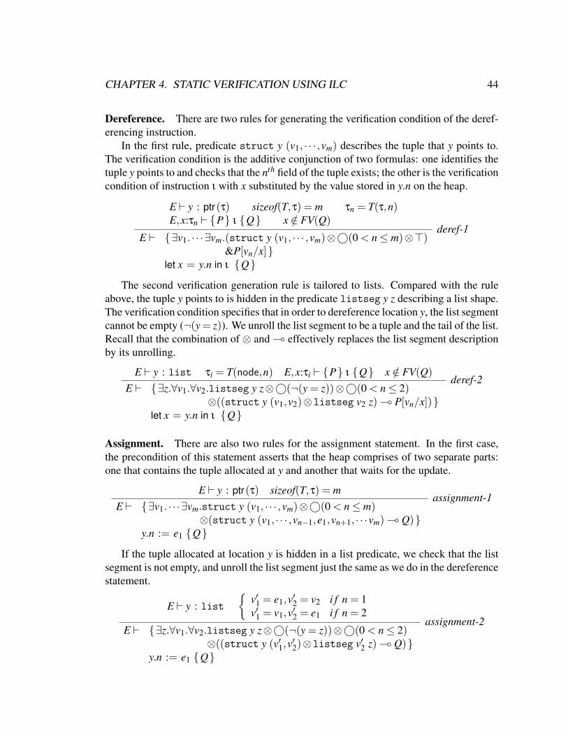
CHAPTER 4. STATIC VERIFICATION USING ILC 44
Dereference. There are two rules for generating the verification condition of the deref-erencing instruction.
In the first rule, predicate struct y (v1, · · · ,vm) describes the tuple that y points to.The verification condition is the additive conjunction of two formulas: one identifies thetuple y points to and checks that the nth field of the tuple exists; the other is the verificationcondition of instruction ι with x substituted by the value stored in y.n on the heap.
E ` y : ptr(τ) sizeof(T,τ) = m τn = T(τ,n)E,x:τn ` P ι Q x /∈ FV(Q)
E ` ∃v1. · · ·∃vm.(struct y (v1, · · · ,vm)⊗©(0 < n≤ m)⊗>)&P[vn/x]
let x = y.n in ι Q
deref-1
The second verification generation rule is tailored to lists. Compared with the ruleabove, the tuple y points to is hidden in the predicate listseg y z describing a list shape.The verification condition specifies that in order to dereference location y, the list segmentcannot be empty (¬(y = z)). We unroll the list segment to be a tuple and the tail of the list.Recall that the combination of ⊗ and ( effectively replaces the list segment descriptionby its unrolling.
E ` y : list τi = T(node,n) E,x:τi ` P ι Q x /∈ FV(Q)E ` ∃z.∀v1.∀v2.listseg y z⊗©(¬(y = z))⊗©(0 < n≤ 2)
⊗((struct y (v1,v2)⊗listseg v2 z) ( P[vn/x])let x = y.n in ι Q
deref-2
Assignment. There are also two rules for the assignment statement. In the first case,the precondition of this statement asserts that the heap comprises of two separate parts:one that contains the tuple allocated at y and another that waits for the update.
E ` y : ptr(τ) sizeof(T,τ) = mE ` ∃v1. · · ·∃vm.struct y (v1, · · · ,vm)⊗©(0 < n≤ m)
⊗(struct y (v1, · · · ,vn−1,e1,vn+1, · · ·vm) ( Q)y.n := e1 Q
assignment-1
If the tuple allocated at location y is hidden in a list predicate, we check that the listsegment is not empty, and unroll the list segment just the same as we do in the dereferencestatement.
E ` y : list
v′1 = e1,v′2 = v2 i f n = 1v′1 = v1,v′2 = e1 i f n = 2
E ` ∃z.∀v1.∀v2.listseg y z⊗©(¬(y = z))⊗©(0 < n≤ 2)⊗((struct y (v′1,v
′2)⊗listseg v′2 z) ( Q)
y.n := e1 Q
assignment-2
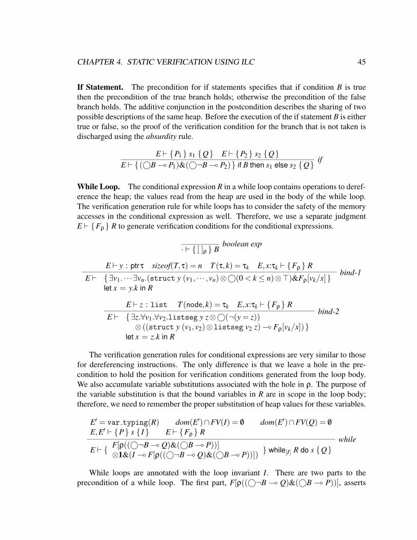
CHAPTER 4. STATIC VERIFICATION USING ILC 45
If Statement. The precondition for if statements specifies that if condition B is truethen the precondition of the true branch holds; otherwise the precondition of the falsebranch holds. The additive conjunction in the postcondition describes the sharing of twopossible descriptions of the same heap. Before the execution of the if statement B is eithertrue or false, so the proof of the verification condition for the branch that is not taken isdischarged using the absurdity rule.
E ` P1 s1 Q E ` P2 s2 QE ` (©B ( P1)&(©¬B ( P2) if B then s1 else s2 Q if
While Loop. The conditional expression R in a while loop contains operations to deref-erence the heap; the values read from the heap are used in the body of the while loop.The verification generation rule for while loops has to consider the safety of the memoryaccesses in the conditional expression as well. Therefore, we use a separate judgmentE ` Fρ R to generate verification conditions for the conditional expressions.
· ` [ ]ρ Bboolean exp
E ` y : ptrτ sizeof(T,τ) = n T (τ,k) = τk E,x:τk ` Fρ R
E ` ∃v1. · · ·∃vn.(struct y (v1, · · · ,vn)⊗©(0 < k ≤ n)⊗>)&Fρ[vk/x]let x = y.k in R
bind-1
E ` z : list T (node,k) = τk E,x:τk ` Fρ R
E ` ∃z.∀v1.∀v2.listseg y z⊗©(¬(y = z))⊗ ((struct y (v1,v2)⊗listseg v2 z) ( Fρ[vk/x])
let x = z.k in R
bind-2
The verification generation rules for conditional expressions are very similar to thosefor dereferencing instructions. The only difference is that we leave a hole in the pre-condition to hold the position for verification conditions generated from the loop body.We also accumulate variable substitutions associated with the hole in ρ. The purpose ofthe variable substitution is that the bound variables in R are in scope in the loop body;therefore, we need to remember the proper substitution of heap values for these variables.
E′ = var typing(R) dom(E′)∩FV(I) = /0 dom(E′)∩FV(Q) = /0
E,E′ ` P s I E ` Fρ R
E ` F[ρ((©¬B ( Q)&(©B ( P))]⊗1&(I ( F[ρ((©¬B ( Q)&(©B ( P))]) while[I] R do s Q
while
While loops are annotated with the loop invariant I. There are two parts to theprecondition of a while loop. The first part, F[ρ((©¬B ( Q)&(©B ( P))], asserts

CHAPTER 4. STATIC VERIFICATION USING ILC 46
that (1), when we execute the loop for the first time, the precondition for evaluatingthe conditional expression, F, must hold; (2), if the loop condition is not true, then thepostcondition Q must hold; and (3), otherwise we will execute the loop body, so theprecondition P for the loop body s must hold. The second part, 1&(I ( F[ρ((©¬B (Q)&(©B ( P))]), asserts that the condition for entering the loop holds each time were-enter the loop. Notice that 1 describes an empty heap. This implies that this invariantcannot depend upon the current heap state.
Function Call. The verification condition of the function call has a similar formula-tion to the verification condition for the assignment statement, except that now we areupdating the footprint of the function.
x /∈ FV(Q) Ψ( f ) = (a:τa ):τ f fb [E f ]Pre∀ret.PostE,x:τ f ` P s Q ∆ = dom(E f )
E ` ∃∆.Pre[e/a]⊗ (∀ret.(Post[e/a] ( P[ret/x]))let x = f (e) in s Q
fun call
The verification condition asserts that the heap consists of two disjoint heaplets. Oneheaplet satisfies the precondition of the function with the parameter substituted with thereal argument, Pre[e/a]. The other heaplet will not be touched by the function. Whenthe second heaplet is merged with the heaplet left by the execution of the function, theverification condition of the subsequent statement s should hold.
4.3.3 Verification Rule for ProgramsFinally, to verify the entire program, we verify each function in the program. We write`ΨOK to denote that all the functions in the domain of Ψ conform to their specified pre-and post-conditions. For each function, a VC is generate from the function’s postcondi-tion using the verification generation rules for function bodies. The last premise of therule check that the function’s precondition entails the VC.
∀ f ∈ dom(Ψ),Ψ( f ) = (a:τa ):τ f fb [E f ]Pre∀ret.Post,dom(E f )∩FV(fb) = /0 a : τa ` V c fb ∀ret.Post Θ;Pre a−=⇒ V c where Θ contains axioms for theories of concern
`ΨOK
4.4 An ExampleIn this section, we use a simple example to demonstrate how to verify programs using theverification condition generation rules defined in the previous section.
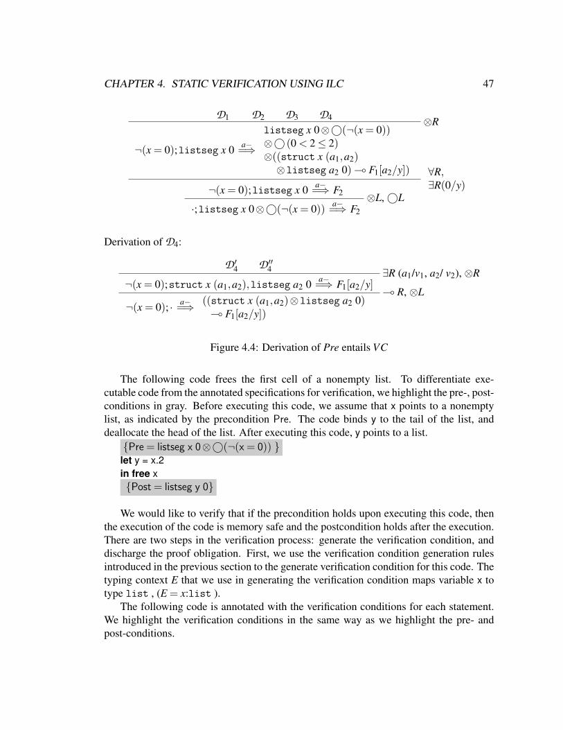
CHAPTER 4. STATIC VERIFICATION USING ILC 47
D1 D2 D3 D4 ⊗R
¬(x = 0);listseg x 0 a−=⇒
listseg x 0⊗©(¬(x = 0))⊗© (0 < 2≤ 2)⊗((struct x (a1,a2)⊗listseg a2 0) ( F1[a2/y]) ∀R,
∃R(0/y)¬(x = 0);listseg x 0 a−=⇒ F2 ⊗L, ©L·;listseg x 0⊗©(¬(x = 0)) a−=⇒ F2
Derivation of D4:
D ′4 D ′′
4 ∃R (a1/v1, a2/ v2), ⊗R¬(x = 0);struct x (a1,a2),listseg a2 0 a−=⇒ F1[a2/y]
( R, ⊗L¬(x = 0); · a−=⇒ ((struct x (a1,a2)⊗listseg a2 0)
( F1[a2/y])
Figure 4.4: Derivation of Pre entails VC
The following code frees the first cell of a nonempty list. To differentiate exe-cutable code from the annotated specifications for verification, we highlight the pre-, post-conditions in gray. Before executing this code, we assume that x points to a nonemptylist, as indicated by the precondition Pre. The code binds y to the tail of the list, anddeallocate the head of the list. After executing this code, y points to a list.
Pre = listseg x 0⊗©(¬(x = 0)) let y = x.2in free xPost = listseg y 0
We would like to verify that if the precondition holds upon executing this code, thenthe execution of the code is memory safe and the postcondition holds after the execution.There are two steps in the verification process: generate the verification condition, anddischarge the proof obligation. First, we use the verification condition generation rulesintroduced in the previous section to the generate verification condition for this code. Thetyping context E that we use in generating the verification condition maps variable x totype list , (E = x:list ).
The following code is annotated with the verification conditions for each statement.We highlight the verification conditions in the same way as we highlight the pre- andpost-conditions.
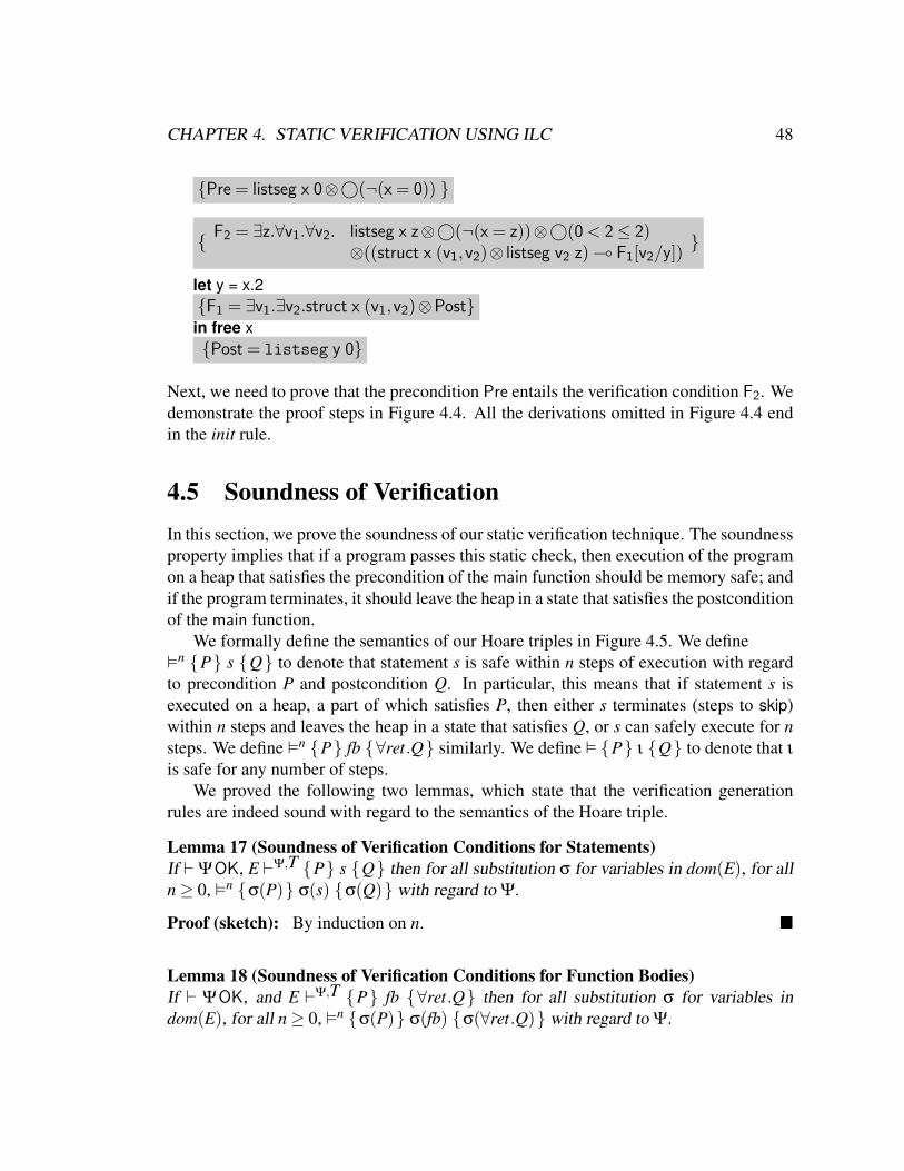
CHAPTER 4. STATIC VERIFICATION USING ILC 48
Pre = listseg x 0⊗©(¬(x = 0))
F2 = ∃z.∀v1.∀v2. listseg x z⊗©(¬(x = z))⊗©(0 < 2≤ 2)⊗((struct x (v1,v2)⊗ listseg v2 z) ( F1[v2/y])
let y = x.2F1 = ∃v1.∃v2.struct x (v1,v2)⊗Postin free xPost = listseg y 0
Next, we need to prove that the precondition Pre entails the verification condition F2. Wedemonstrate the proof steps in Figure 4.4. All the derivations omitted in Figure 4.4 endin the init rule.
4.5 Soundness of VerificationIn this section, we prove the soundness of our static verification technique. The soundnessproperty implies that if a program passes this static check, then execution of the programon a heap that satisfies the precondition of the main function should be memory safe; andif the program terminates, it should leave the heap in a state that satisfies the postconditionof the main function.
We formally define the semantics of our Hoare triples in Figure 4.5. We definen P s Q to denote that statement s is safe within n steps of execution with regardto precondition P and postcondition Q. In particular, this means that if statement s isexecuted on a heap, a part of which satisfies P, then either s terminates (steps to skip)within n steps and leaves the heap in a state that satisfies Q, or s can safely execute for nsteps. We define n P fb ∀ret.Q similarly. We define P ι Q to denote that ι
is safe for any number of steps.We proved the following two lemmas, which state that the verification generation
rules are indeed sound with regard to the semantics of the Hoare triple.
Lemma 17 (Soundness of Verification Conditions for Statements)If `ΨOK, E `Ψ,T P s Q then for all substitution σ for variables in dom(E), for alln≥ 0, n σ(P) σ(s) σ(Q) with regard to Ψ.
Proof (sketch): By induction on n.
Lemma 18 (Soundness of Verification Conditions for Function Bodies)If ` ΨOK, and E `Ψ,T P fb ∀ret.Q then for all substitution σ for variables indom(E), for all n≥ 0, n σ(P) σ(fb) σ(∀ret.Q) with regard to Ψ.
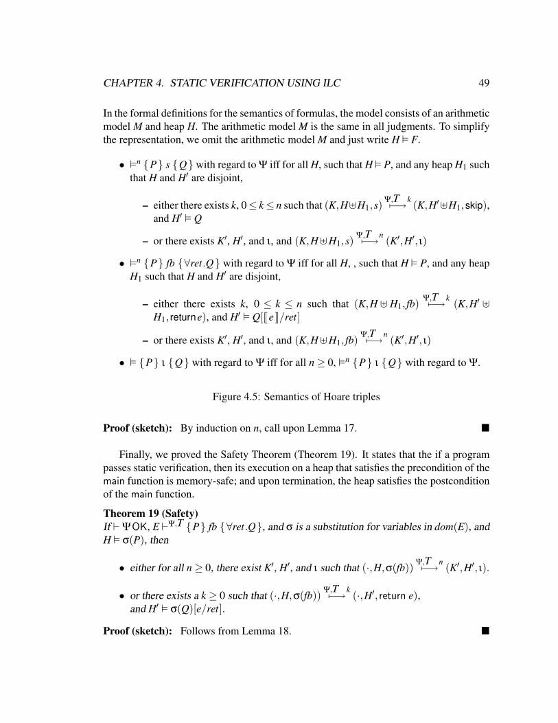
CHAPTER 4. STATIC VERIFICATION USING ILC 49
In the formal definitions for the semantics of formulas, the model consists of an arithmeticmodel M and heap H. The arithmetic model M is the same in all judgments. To simplifythe representation, we omit the arithmetic model M and just write H F.
• n P s Q with regard to Ψ iff for all H, such that H P, and any heap H1 suchthat H and H′ are disjoint,
– either there exists k, 0≤ k≤ n such that (K,H]H1,s)Ψ,T k7−→ (K,H′]H1,skip),
and H′ Q
– or there exists K′, H′, and ι, and (K,H]H1,s)Ψ,T n7−→ (K′,H′, ι)
• n P fb ∀ret.Q with regard to Ψ iff for all H, , such that H P, and any heapH1 such that H and H′ are disjoint,
– either there exists k, 0 ≤ k ≤ n such that (K,H ] H1, fb)Ψ,T k7−→ (K,H′ ]
H1, returne), and H′ Q[JeK/ret]
– or there exists K′, H′, and ι, and (K,H]H1, fb)Ψ,T n7−→ (K′,H′, ι)
• P ι Q with regard to Ψ iff for all n≥ 0, n P ι Q with regard to Ψ.
Figure 4.5: Semantics of Hoare triples
Proof (sketch): By induction on n, call upon Lemma 17.
Finally, we proved the Safety Theorem (Theorem 19). It states that the if a programpasses static verification, then its execution on a heap that satisfies the precondition of themain function is memory-safe; and upon termination, the heap satisfies the postconditionof the main function.
Theorem 19 (Safety)If `ΨOK, E `Ψ,T P fb ∀ret.Q, and σ is a substitution for variables in dom(E), andH σ(P), then
• either for all n≥ 0, there exist K′, H′, and ι such that (·,H,σ(fb))Ψ,T n7−→ (K′,H′, ι).
• or there exists a k ≥ 0 such that (·,H,σ(fb))Ψ,T k7−→ (·,H′, return e),
and H′ σ(Q)[e/ret].
Proof (sketch): Follows from Lemma 18.

CHAPTER 4. STATIC VERIFICATION USING ILC 50
init¬(p = 0)¬(n = 0);listseg x 0 a−=⇒ listseg x 0
list-4¬(p = 0)¬(n = 0);listseg x p,listseg p 0 a−=⇒ listseg x 0
list-1’¬(p = 0)¬(n = 0) ;
listseg x p,struct p (d p,n),listseg n 0
a−=⇒ listseg x 0list-1’
¬(p = 0)¬(n = 0) ;
listseg x p,struct p (d p,n),listseg q 0,struct n (3,q)
a−=⇒ listseg x 0inequality
·;listseg x p,struct p (d p,n),listseg q 0,struct n (3,q)
a−=⇒ listseg x 0
Figure 4.6: Derivation for example insertion
4.6 Further ExamplesIn this section, we present three examples of statically verifying programs that performcommonly used list operations. These examples demonstrate how the predicate describ-ing the list data structure are unrolled and how formulas describing pieces of a list arerolled back to a list as the programs traverse the data structure using while loops andrecursive function calls. In order to roll or unroll the list descriptions, we use the proofrules introduced in the Section 3.4.
Insertion. The following code inserts a new key into a list that starts from location x.After insertion, the new key will be the successor of pointer p. To insert the new node afterpointer p, we allocate a tuple of node type for the new key, link the next field of p to thisnew tuple, and link the next field of the new tuple to p’s old next field. The preconditiondescribes the shape of the list before executing the program. The postcondition specifiesthat after the insertion x still points to a list.
Pre = listseg x p⊗ struct p (dp,q)⊗ listseg q 0let n = new(sizeof(node))in p.2:=n
n.1:=3;n.2:=q
Post = listseg x 0
The process of verification condition generation is straightforward. We focus on howto discharge the proof obligations. The main subgoal of the proof is that after inserting thenew tuple, x still points to a list. We present the derivation of this subgoal in Figure 4.6.Notice that we need to fold two lists together using the list-4 rule.
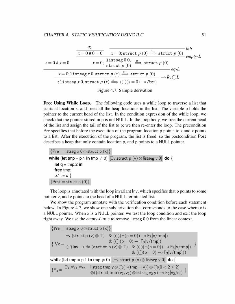
CHAPTER 4. STATIC VERIFICATION USING ILC 51
x = 0 # x = 0
D1x = 0 # 0 = 0
initx = 0;struct p (0) a−=⇒ struct p (0)
empty-Lx = 0;
listseg 0 0,struct p (0)
a−=⇒ struct p (0)eq-L
x = 0;listseg x 0,struct p (x) a−=⇒ struct p (0)( R, ©L
·;listseg x 0,struct p (x) a−=⇒ (©(x = 0) ( Post)
Figure 4.7: Sample derivation
Free Using While Loop. The following code uses a while loop to traverse a list thatstarts at location x, and frees all the heap locations in the list. The variable p holds thepointer to the current head of the list. In the condition expression of the while loop, wecheck that the pointer stored in p is not NULL. In the loop body, we free the current headof the list and assign the tail of the list to p; we then re-enter the loop. The preconditionPre specifies that before the execution of the program location p points to x and x pointsto a list. After the execution of the program, the list is freed, so the postcondition Postdescribes a heap that only contain location p, and p points to a NULL pointer.
Pre = listseg x 0⊗ struct p (x)while (let tmp = p.1 in tmp 6= 0) [∃v.struct p (v)⊗ listseg v 0] do
let q = tmp.2 infree tmp;p.1 := q
Post = struct p (0)
The loop is annotated with the loop invariant Inv, which specifies that p points to somepointer v, and v points to the head of a NULL-terminated list.
We show the program annotate with the verification condition before each statementbelow. In Figure 4.7, we show one subderivation that corresponds to the case where x isa NULL pointer. When x is a NULL pointer, we test the loop condition and exit the loopright away. We use the empty-L rule to remove listseg 0 0 from the linear context.
Pre = listseg x 0⊗ struct p (x)
Vc =
∃v.(struct p (v)⊗>) & (©(¬(p = 0)) ( F3[v/tmp])& (©(p = 0) ( F3[v/tmp])
⊗!(Inv ( ∃v.(struct p (v)⊗>) & (©(¬(p = 0)) ( F3[v/tmp])& (©(p = 0) ( F3[v/tmp]))
while (let tmp = p.1 in tmp 6= 0) [∃v.struct p (v)⊗ listseg v 0] do
F3 =∃y.∀v1.∀v2. listseg tmp y⊗©(¬(tmp = y))⊗©(0 < 2≤ 2)
⊗((struct tmp (v1,v2)⊗ listseg v2 y) ( F2[v2/q])
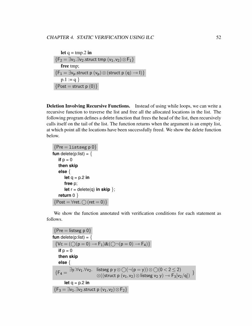
CHAPTER 4. STATIC VERIFICATION USING ILC 52
let q = tmp.2 inF2 = ∃v1.∃v2.struct tmp (v1,v2)⊗F1
free tmp;F1 = ∃vp.struct p (vp)⊗ (struct p (q) ( I)
p.1 := q Post = struct p (0)
Deletion Involving Recursive Functions. Instead of using while loops, we can write arecursive function to traverse the list and free all the allocated locations in the list. Thefollowing program defines a delete function that frees the head of the list, then recursivelycalls itself on the tail of the list. The function returns when the argument is an empty list,at which point all the locations have been successfully freed. We show the delete functionbelow.
Pre = listseg p 0fun delete(p:list) =
if p = 0then skipelse
let q = p.2 infree p;let r = delete(q) in skip ;
return 0 Post = ∀ret.© (ret = 0)
We show the function annotated with verification conditions for each statement asfollows.
Pre = listseg p 0fun delete(p:list) = Vc = (©(p = 0) ( F1)&(©¬(p = 0) ( F4)
if p = 0then skipelse
F4 =∃y.∀v1.∀v2. listseg p y⊗©(¬(p = y))⊗©(0 < 2≤ 2)
⊗((struct p (v1,v2)⊗ listseg v2 y) ( F3[v2/q])
let q = p.2 inF3 = ∃v1.∃v2.struct p (v1,v2)⊗F2
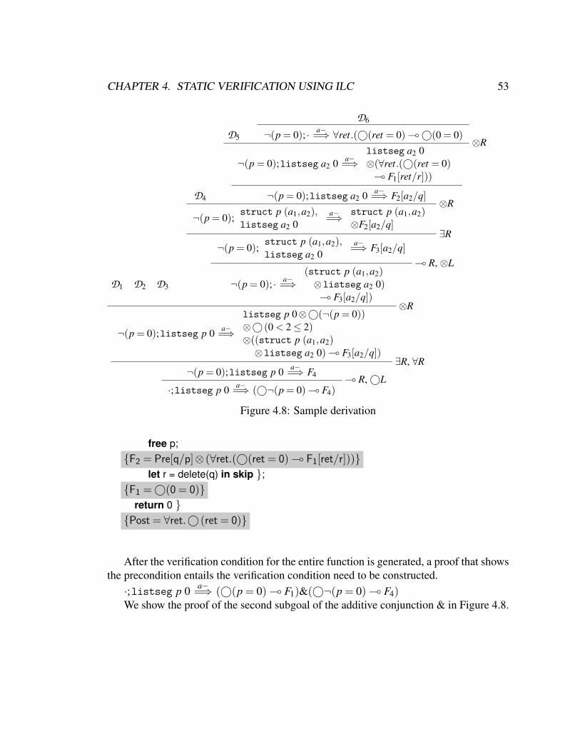
CHAPTER 4. STATIC VERIFICATION USING ILC 53
D1 D2 D3
D4
D5
D6
¬(p = 0); · a−=⇒ ∀ret.(©(ret = 0) (©(0 = 0)⊗R
¬(p = 0);listseg a2 0 a−=⇒listseg a2 0⊗(∀ret.(©(ret = 0)
( F1[ret/r]))
¬(p = 0);listseg a2 0 a−=⇒ F2[a2/q]⊗R
¬(p = 0);struct p (a1,a2),listseg a2 0
a−=⇒ struct p (a1,a2)⊗F2[a2/q]
∃R¬(p = 0);
struct p (a1,a2),listseg a2 0
a−=⇒ F3[a2/q]( R, ⊗L
¬(p = 0); · a−=⇒(struct p (a1,a2)⊗listseg a2 0)( F3[a2/q])
⊗R
¬(p = 0);listseg p 0 a−=⇒
listseg p 0⊗©(¬(p = 0))⊗© (0 < 2≤ 2)⊗((struct p (a1,a2)⊗listseg a2 0) ( F3[a2/q])
∃R, ∀R¬(p = 0);listseg p 0 a−=⇒ F4
( R, ©L·;listseg p 0 a−=⇒ (©¬(p = 0) ( F4)
Figure 4.8: Sample derivation
free p;F2 = Pre[q/p]⊗ (∀ret.(©(ret = 0) ( F1[ret/r]))
let r = delete(q) in skip ;F1 =©(0 = 0)
return 0 Post = ∀ret.© (ret = 0)
After the verification condition for the entire function is generated, a proof that showsthe precondition entails the verification condition need to be constructed.
·;listseg p 0 a−=⇒ (©(p = 0) ( F1)&(©¬(p = 0) ( F4)We show the proof of the second subgoal of the additive conjunction & in Figure 4.8.

Chapter 5
Dynamic Heap-shape Contracts
In this chapter, we explore using contracts to dynamically check the shape properties ofthe program heap (e.g. the invariants of data structures). Contracts are specifications thatprogrammers use to document component requirements and to clearly express guarantees.More precisely, contracts are executable specifications that are evaluated at run timeto enforce the specified properties. People have studied and used contracts since the1970s [60, 34, 50, 52]. In Eiffel for instance, programmers can specify the pre- and post-condition of an object’s method. When used consistently, contracts can help improve theclarity of code and detect programmer errors. All kinds of past and current languagesinclude these features, including Eiffel [51], Java [64] and Scheme [20].
We develop a contract-based dynamic verification system that uses the same logicalinfrastructure as the static verification system presented in the previous chapter. Whenused as contracts, logical specifications are much lighter-weight verification mechanismsthan when used in static verification. A programmer can simply place a contract wherevershe chooses in her program, employing a pay-as-you-go strategy for making her programsmore reliable. More importantly, we can seamlessly combine these two verificationmethods because they use a unified specification language. The users can balance thestrengths and weaknesses of dynamic and static verification methods in one system.
5.1 Using Formal Logic as a Contract LanguageMost contract systems expect programmers to use the native programming language toexpress their program invariants. While this technique is most effective for many simpleinvariants, expressing properties of data structures can be extremely complicated. Infact, any naive “roll your own” function a programmer might write to check heap-shapeproperties would have to set up substantial infrastructure to record and check aliasingproperties. If this infrastructure is set up in an ad hoc, verbose, and unstructured manner,the meaning of contracts will be unclear and their value as documentation substantiallydiminished.
54
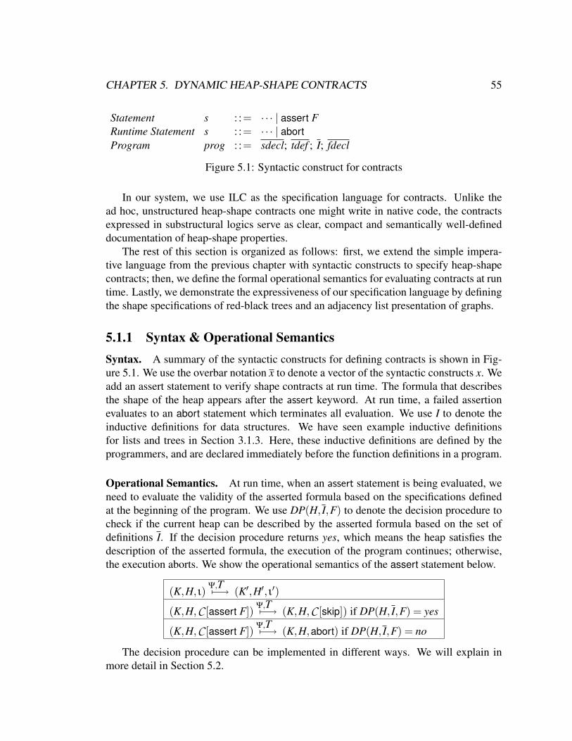
CHAPTER 5. DYNAMIC HEAP-SHAPE CONTRACTS 55
Statement s : := · · · | assert FRuntime Statement s : := · · · | abortProgram prog : := sdecl; tdef ; I; fdecl
Figure 5.1: Syntactic construct for contracts
In our system, we use ILC as the specification language for contracts. Unlike thead hoc, unstructured heap-shape contracts one might write in native code, the contractsexpressed in substructural logics serve as clear, compact and semantically well-defineddocumentation of heap-shape properties.
The rest of this section is organized as follows: first, we extend the simple impera-tive language from the previous chapter with syntactic constructs to specify heap-shapecontracts; then, we define the formal operational semantics for evaluating contracts at runtime. Lastly, we demonstrate the expressiveness of our specification language by definingthe shape specifications of red-black trees and an adjacency list presentation of graphs.
5.1.1 Syntax & Operational SemanticsSyntax. A summary of the syntactic constructs for defining contracts is shown in Fig-ure 5.1. We use the overbar notation x to denote a vector of the syntactic constructs x. Weadd an assert statement to verify shape contracts at run time. The formula that describesthe shape of the heap appears after the assert keyword. At run time, a failed assertionevaluates to an abort statement which terminates all evaluation. We use I to denote theinductive definitions for data structures. We have seen example inductive definitionsfor lists and trees in Section 3.1.3. Here, these inductive definitions are defined by theprogrammers, and are declared immediately before the function definitions in a program.
Operational Semantics. At run time, when an assert statement is being evaluated, weneed to evaluate the validity of the asserted formula based on the specifications definedat the beginning of the program. We use DP(H, I,F) to denote the decision procedure tocheck if the current heap can be described by the asserted formula based on the set ofdefinitions I. If the decision procedure returns yes, which means the heap satisfies thedescription of the asserted formula, the execution of the program continues; otherwise,the execution aborts. We show the operational semantics of the assert statement below.
(K,H, ι)Ψ,T7−→ (K′,H′, ι′)
(K,H,C [assert F])Ψ,T7−→ (K,H,C [skip]) if DP(H, I,F) = yes
(K,H,C [assert F])Ψ,T7−→ (K,H,abort) if DP(H, I,F) = no
The decision procedure can be implemented in different ways. We will explain inmore detail in Section 5.2.

CHAPTER 5. DYNAMIC HEAP-SHAPE CONTRACTS 56
5.1.2 Example SpecificationsTo demonstrate the expressiveness of our specification language, we have used it to definemany commonly used data structures such as lists, circular lists, trees, B-trees, red-blacktress, and an adjacency list representation for graphs. In this section, we show how todefine two complex data structures: red-black trees and an adjacency list representationof graphs.
Red-Black Trees. Red-black trees are balanced binary search trees. To specify theinvariants of red-black trees, we not only need to specify its tree shape, but also need tospecify that the key on the right child is less than the key on the root, that the key on theleft child is greater than the key on the root, that red nodes do not have red parents, andthat the black heights of all leaves are equal.
We define an auxiliary predicate, checkData, to describe the ordering between thedata D of the current node and the data Pd of the parent node. The checkData predicatealso takes a flag Rc to indicate whether this node is a left child (Rc = 0), a right child (Rc= 1), or the special case, the root (Rc = 2).
checkData D Pd Rc o–O(Rc = 0), (O(D = Pd); O(Pd >D));O(Rc = 1), (O(D = Pd); O(D >Pd));O(Rc = 2).
We next define the predicate rnode L Pd Rc Bh to describe a red node that starts ataddress L. The argument Bh is the black height of all the leaves under this node. Thearguments Pd and Rc have the same meaning as above. The definition of the red node isgiven below.
rnode L Pd Rc Bh o–struct L (1,Data,Left,Right), checkData Data Pd Rc,bnode Left Data 0 Bh, bnode Right Data 1 Bh.
A red node contains four data fields: the color red (represented by 1), data, andpointers to a left child and a right child. A well-formed red node requires that the datais appropriately related to that of its parent, that both the left and right children are blacknodes, and that the black height of the two subtrees is equal.
We now define black nodes and nodes of either color.
bnode L Pd Rc Bh o–(O(L = 0), O(Bh = 0));

CHAPTER 5. DYNAMIC HEAP-SHAPE CONTRACTS 57
0
0
0100
200
300
200
300
0
410 510
510410
610
200 300
300610
a
cb
(a)
(b)
(c)
Figure 5.2: An adjacency list.
(struct L (0,Data,Left,Right), checkData Data Pd Rc,rbnode Left Data 0 Bh2, rbnode Right Data 1 Bh2, O(Bh = Bh2 + 1)).
rbnode L Pd Rc Bh o–bnode L Pd Rc Bh; rnode L Pd Rc Bh.
A black node is similar to a red node. The first subformula of the disjunction in thebody describes a leaf node, which is the NULL pointer, and its black height 0. The secondsubformula of the disjunction describes a black node whose two children have the sameblack height and can be of either color. The black height of the root node is the children’sblack hight increases by one.
The location L is a pointer to a red-black tree (rbtree L) if it is a black node of someblack height.
rbtree L o–bnode L 0 2 Bh.
Adjacency List Presentation of Graphs. Adjacency lists are one of the most com-monly used data structures for representing graphs. In Figure 5.2, the data structure onthe left is an adjacency list representation of the directed graph on the right. Each node inthe graph is represented as a tuple composed of three fields. The first field is a data field;the second field is a pointer to another node in the graph, and the last field is a pointer tothe adjacency list of outgoing edges. In this example, node a is represented by the tuplestarting at address 100, b is represented by the one starting at 200, and c is representedby the one starting at 300. In this data structure, each tuple representing a graph nodeis pointed to from the previous node and from the node’s incoming edges. For example,node c (tuple starting at address 300) is pointed to by the next pointer from node b, andfrom the adjacency lists of both node a and b.
We present the definitions of an adjacency list in Figure 5.3. At the bottom ofFigure 5.3, we define predicate adjlist X B. This predicate describes the list of outgoingedges from a node. The argument X points to the beginning of the list and the argumentB represents the set of nodes contained therein.
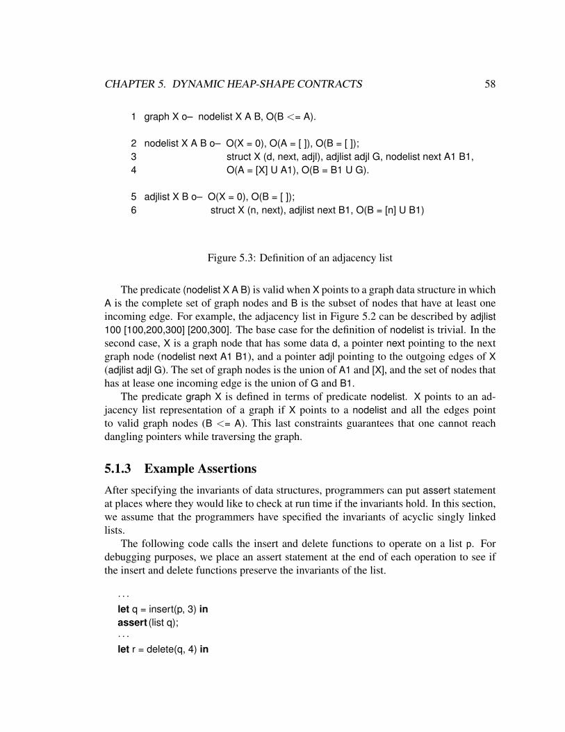
CHAPTER 5. DYNAMIC HEAP-SHAPE CONTRACTS 58
1 graph X o– nodelist X A B, O(B <= A).
2 nodelist X A B o– O(X = 0), O(A = [ ]), O(B = [ ]);3 struct X (d, next, adjl), adjlist adjl G, nodelist next A1 B1,4 O(A = [X] U A1), O(B = B1 U G).
5 adjlist X B o– O(X = 0), O(B = [ ]);6 struct X (n, next), adjlist next B1, O(B = [n] U B1)
Figure 5.3: Definition of an adjacency list
The predicate (nodelist X A B) is valid when X points to a graph data structure in whichA is the complete set of graph nodes and B is the subset of nodes that have at least oneincoming edge. For example, the adjacency list in Figure 5.2 can be described by adjlist100 [100,200,300] [200,300]. The base case for the definition of nodelist is trivial. In thesecond case, X is a graph node that has some data d, a pointer next pointing to the nextgraph node (nodelist next A1 B1), and a pointer adjl pointing to the outgoing edges of X(adjlist adjl G). The set of graph nodes is the union of A1 and [X], and the set of nodes thathas at lease one incoming edge is the union of G and B1.
The predicate graph X is defined in terms of predicate nodelist. X points to an ad-jacency list representation of a graph if X points to a nodelist and all the edges pointto valid graph nodes (B <= A). This last constraints guarantees that one cannot reachdangling pointers while traversing the graph.
5.1.3 Example AssertionsAfter specifying the invariants of data structures, programmers can put assert statementat places where they would like to check at run time if the invariants hold. In this section,we assume that the programmers have specified the invariants of acyclic singly linkedlists.
The following code calls the insert and delete functions to operate on a list p. Fordebugging purposes, we place an assert statement at the end of each operation to see ifthe insert and delete functions preserve the invariants of the list.
· · ·let q = insert(p, 3) inassert (list q);· · ·let r = delete(q, 4) in
CHAPTER 5. DYNAMIC HEAP-SHAPE CONTRACTS 59
assert (list r);· · ·
In the next example, the merge function merge two disjoint lists into one. We wouldlike to make sure that the arguments passed to the merge function are indeed two disjointlists.
fun merge(p,q) = assert (list p, list q)· · ·
Recall that the comma in formula (list p, list q) is the multiplicative conjunction. There-fore, if the assertion succeeds, we know that list p and list q belong to two separate partsof the heap.
5.2 ImplementationWe have implemented heap-shape contracts on a fragment of ANSI-C [61], which we callMiniC. In this section, we explain how to implement heap-shape contracts on MiniC. Inparticular, first we introduce the MiniC language and describe our implementation of aninterpreter for MiniC. Then, we explain how we implemented the procedure for checkingthe validity of assertions using LolliMon, a linear logic programming language; and howwe used mode-analysis to achieve efficiency. Lastly, we explain how we could implementsuch a system on ANSI-C via source-to-source translation to C in the future 1.
5.2.1 The MiniC LanguageMiniC is a subset of C that includes basic control flow constructs, pointers, structs,unions, and enums with the addition of inductive definitions and assert statements.
A MiniC program begins with a set of clause definitions. The implementation auto-matically includes some basic predicates such as struct. Next, a sequence of top leveldeclarations declare global variables, struct and union definitions, type definitions, func-tion declarations, and enumerations. The final piece of every MiniC program is a mainfunction. We extend the syntax of the assert statement to take the logical formula to beasserted.
Our implementation consists of a simple lexer, parser, and interpreter for the MiniC.The MiniC interpreter is written in OCaml. It is completely standard, except for theinterpretation of assert statements. When an assert is reached, it calls the logic engine
1The interpreter for MiniC is implemented by Frances Perry. I modified LolliMon to make memoryaccess more efficient, and implemented the interface to link LolliMon to the interpreter.
CHAPTER 5. DYNAMIC HEAP-SHAPE CONTRACTS 60
to verify the asserted formula. We implemented an interface to a modified version of alinear logic programming language, LolliMon [49] to decide the validity of assertions.
5.2.2 Checking AssertionsWhen an assertion is encountered, LolliMon is called to check the validity of the assertedformula. Because LolliMon is a light-weight linear logic theorem prover, the evaluationof the validity of the asserted formula is conceptually a proof search of this assertedformula against the logical encoding of the heap and the shape definitions. We obtain thelogical encoding of the current heap in such a way that the current program heap makesup the linear context that consists of the basic descriptions for each location on the heap;and the logical specifications make up the unrestricted context. The backward-chainingoperational semantics of LolliMon gives a natural interpretation of the logical connectivesas goal-directed search instructions. If we peek into the run time of LolliMon when it ischecking a list predicate, the logic engine traverses the list in almost the same way as a Cfunction would do. Finally, because of the soundness result (described in Theorems 6, 7),we know that if LolliMon found a proof then the asserted formula is valid.
In our implementation, we modified LolliMon so that LolliMon uses the program’snative heap directly instead of encoding the heap in the linear logical context.
5.2.3 Mode AnalysisWe use mode analysis to guide the evaluation of the asserted formulas for efficient eval-uation. To understand the purpose of mode analysis, consider the problem of matchingthe predicate struct X (77,34) against the contents of some heap H. Logically, the goalof the matching algorithm is to find an address l such that H( l) = (77,34). However,without any additional information, it would seem the only possible algorithm wouldinvolve examining the contents of every address in the entire heap H until finding one thatsatisfies the constraint is found. In general however, attempting to use such an algorithmin practice would be hopelessly inefficient.
On the other hand, suppose we are given a specific address l’ and we would like tomatch the formula (struct l′ (D,X),struct X (77,34)) against some heap H. We can simplylook up l’ in H to determine values for D and X. The value of X is subsequently used todetermine whether H(X) = (77,34). We also need to ensure the value of X is not equalto l’ (otherwise the linearity constraint that l’ and X point to disjoint heaplets would beviolated).
When a value such as l’ or X is known, it is referred to as ground. Mode declarationsspecify, among other things, expectations concerning which arguments are ground inwhich positions. Finally, mode analysis is a syntactic analysis, much like type checking,that can determine whether the mode declarations are correct.
CHAPTER 5. DYNAMIC HEAP-SHAPE CONTRACTS 61
In our system, the modes for specifying groundness conditions are the standard onesfound in many logic programming languages such as Prolog. In particular, the inputmode (+) specifies that a term in that position must be ground before evaluation of thepredicate. The output mode (-) specifies the term in that position must be ground termafter the predicate is evaluated. The last mode (*) indicates that there is no restrictionof the argument in this position. Now, to guarantee that it is possible to evaluate thepredicate struct X (...) in constant time, we give the first position (X) the input mode (+).Once the first argument of the struct predicate has been constrained to have input mode,other definitions that use it are constrained in turn. For example, the first argument oflist X must also be inputs.
In the specification of the invariants of data structures, programmers are also requiredto declare the correct modes for predicates. LolliMon’s mode analysis will check if allthe inductive definitions are well-moded at compile time. When all the inductive defini-tions are well-moded, the decision procedure that checks whether the asserted formulasdescribe the current heap can take advantage of this information and makes checking thepredicate struct X (...) a constant-time operation.
5.2.4 Source to Source TranslationOne way to implement this dynamic verification system for ANSI-C is to develop asource-to-source translation algorithm that converts a C program with logical assertionsto an equivalent plain C program. In this section, we discuss the issues involved indeveloping such a source-to-source translation algorithm.
Decision Procedures for Checking the Validity of Formulas. The main part of thissource-to-source translation algorithm is to automatically generate C code that decide thevalidity of logical formulas based on user-defined logical specifications. We can convertthe clauses defining the data structures into functions that traverse the heap and keeptrack of heap locations that have been visited to preserve linearity. We will explain howto generate such a decision procedure in Chapter 6.
In the implementation of the verification system in our conference paper [61], theasserted formula describes the entire program heap. For example, if we assert list x,this means that x points to a list and it is the only data structure allocated on the heap.The interpreter manages the internal state of the program heap, making it easy to verifythe validity of the formulas against the entire heap. However, this is impossible to do ina source-to-source translation.
However, the most practical use of these dynamic assertions is to verify the invariantsgoverning a simple data structure instead of the shape of the entire allocated heap. Inother words, we only want to know if x points to a list. This means that given an assertionformula F, we are verifying if H F⊗> instead of HF. In this case, we simply invoke
CHAPTER 5. DYNAMIC HEAP-SHAPE CONTRACTS 62
the C function automatically generated from the user-defined specifications to traversethe heap.
Handling Exceptions. In the current implementation, LolliMon throws an exceptionwhen the assertion fails. The interpreter catches this exception, prints out error messagesand terminates the execution of the program. ANSI-C does not support exception han-dling directly. However, there are libraries available that implement exception handlingusing the “setjump” and “longjump” commands. In a source-to-source translation, whenthe assertion fails, we could either simply exit the program or use more sophisticatedexception handling libraries to handle the failure of assertions.
5.3 Combining Static and Dynamic VerificationStatic verification and dynamic verification both have their advantages and disadvantages.The costs of implementing each system also differ. In this section, we discuss the prop-erties of each system and show how we can combine them.
The static verification method introduced in the previous chapter performs compile-time analysis on the entire program. In addition to providing memory-safety guaranteeson all paths of execution, it ensures that the precondition holds before the execution ofeach function; and that the post-condition holds after the execution of the function. Sinceit is a compile time check, no run-time performance penalty is incurred. The complexityof deploying such a system includes: (1), discovering the right set of axioms to reasonabout different data structures; (2), developing complex theorem provers to dischargeproof obligations; and (3), annotating programs with proper pre- and post-conditions andloop invariants. Because of the complexity of developing theorem provers and annotatingprograms with appropriate invariants, it is often expensive to use the static verificationmethod only, if possible at all. We often find ourselves in situations where we do nothave access to the entire code base, or there is not a theorem prover available that candischarge the proof obligations.
On the other hand, dynamic verification is comparatively easier to implement. Thereis no complicated theorem proving involved. Programmers can place the assertionswherever they need to. However, there is run-time cost added to the program. It isrelatively simple to check that the pre- and post-condition of functions hold by placingassertions of the precondition at the entry point of the function and placing the post-condition before return. However, it is hard to check certain memory-safety propertiessuch as no-dangling-pointer dereferencing using only dynamic assertions. Analyzingsuch properties often requires information about the evaluation history of the program,while dynamic checks typically have access only to a snapshot of the heap. Furthermore,whenever an assertion fails, there is extra work to be done to deal with error handling.

CHAPTER 5. DYNAMIC HEAP-SHAPE CONTRACTS 63
We can mitigate the cost of verification by combining static and dynamic verificationmethods. For instance, we could dedicate more resources to statically verify a smallbut critical portion of the program. In order for this method to be sound, we also need tomake sure that upon entering these statically verified functions the required preconditionsare met. We could ensure this by inserting dynamic checks at the entry points of thefunctions. If the precondition does not hold at the entry point, then an exception is thrownand no improper pointer operations will be performed.
The most effective way to develop a verification system that combines static anddynamic verification is to use one unified specification language for both systems. Boththe static verification system from the previous chapter and the dynamic verificationsystem here use ILC as the specification language for describing the invariants of datastructures. Therefore, we can easily combine these two systems. If we wish to check atrun time that the precondition of a function holds upon entering the function body, wecan simply assert the precondition using the assert statement as the first statement beforeentering the function.
For example, the delete function in Section 4.6 assumes that the argument passedin is a list. If the argument passed in is not a list, the delete function will not properlyfree all allocated heap cells. Assume we statically verified this delete function already.We then only need to write a wrapper function, and add an assert statement as the firststatement of this wrapper function before calling the verified delete function. We showthe del function and the wrapper function delete below. Using this technique we knowthat whenever the statically verified del function is called, it is operating on a list.
fun delete(p) = assert (list p);let r = del(p) inreturn r
Pre = listseg p 0fun del(p:list) =
if p = 0then skipelse let q = p.2
in free p;let r = del(q) in
skip;return 0
Post = ∀ret.© (ret = 0)

Chapter 6
Shape Patterns
In this chapter, we present a new programming paradigm designed to incorporate verifi-cation techniques into the language. In our language, which we call the pattern language,programmers construct data structures by specifying the shapes they want at a high levelof abstraction, using linear logical formulas rather than low-level pointer operations.Likewise, programmers deconstruct data structures using a new form of pattern matching,in which the patterns are again drawn from the syntax of linear logic. Rather thansupporting a two-step program-then-verify paradigm, we support a one-step correct-by-construction process.
Using declarative logical formulas to construct and deconstruct data structures comesnaturally from the way we study these data structures. Regardless of the language used,the first step of coding is often to draw a sketch to represent the scenario, e.g. as is shownbelow for a list insert function.
npx
In this picture, x points to the beginning of the list, and n points to the new cell to beinserted behind p. The picture contains precise descriptions of the list before and after theinsertion operation. When using C, we discard some of the invariants described by thepicture and translate the picture into C’s pointer dereferencing and assignment, as shownbelow.
n –>next = p –>nextp –>next = n
In our pattern language, the logical shape patterns match much more closely with thedescriptions of the data structures in those pictures. First, we examine the shape of thelist before the insertion using a shape pattern as follows.
64
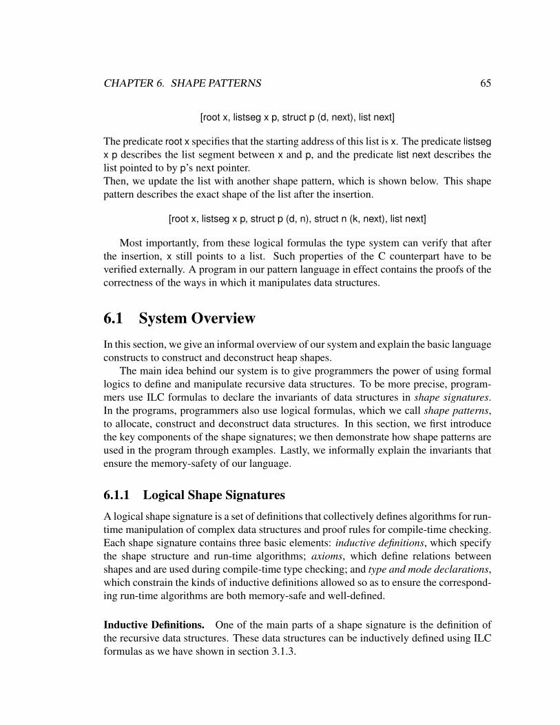
CHAPTER 6. SHAPE PATTERNS 65
[root x, listseg x p, struct p (d, next), list next]
The predicate root x specifies that the starting address of this list is x. The predicate listsegx p describes the list segment between x and p, and the predicate list next describes thelist pointed to by p’s next pointer.Then, we update the list with another shape pattern, which is shown below. This shapepattern describes the exact shape of the list after the insertion.
[root x, listseg x p, struct p (d, n), struct n (k, next), list next]
Most importantly, from these logical formulas the type system can verify that afterthe insertion, x still points to a list. Such properties of the C counterpart have to beverified externally. A program in our pattern language in effect contains the proofs of thecorrectness of the ways in which it manipulates data structures.
6.1 System OverviewIn this section, we give an informal overview of our system and explain the basic languageconstructs to construct and deconstruct heap shapes.
The main idea behind our system is to give programmers the power of using formallogics to define and manipulate recursive data structures. To be more precise, program-mers use ILC formulas to declare the invariants of data structures in shape signatures.In the programs, programmers also use logical formulas, which we call shape patterns,to allocate, construct and deconstruct data structures. In this section, we first introducethe key components of the shape signatures; we then demonstrate how shape patterns areused in the program through examples. Lastly, we informally explain the invariants thatensure the memory-safety of our language.
6.1.1 Logical Shape SignaturesA logical shape signature is a set of definitions that collectively defines algorithms for run-time manipulation of complex data structures and proof rules for compile-time checking.Each shape signature contains three basic elements: inductive definitions, which specifythe shape structure and run-time algorithms; axioms, which define relations betweenshapes and are used during compile-time type checking; and type and mode declarations,which constrain the kinds of inductive definitions allowed so as to ensure the correspond-ing run-time algorithms are both memory-safe and well-defined.
Inductive Definitions. One of the main parts of a shape signature is the definition ofthe recursive data structures. These data structures can be inductively defined using ILCformulas as we have shown in section 3.1.3.
CHAPTER 6. SHAPE PATTERNS 66
Axioms. Each shape signature can contain many inductive definitions. For instance,the listshape signature, which we will be using as a running example through this chapterwill contain the definitions of both list and listseg. In order to allow the system to reasonabout the relationships between these various definitions, the programmer must writedown additional clauses, which we call axioms. For example, the following axiom relateslist to listseg.
list Y o− listseg Y Z, list Z.
Without this axiom, the type system cannot prove that one complete shape, such as (listsegx y, list y), is related to another (list x).
Type and Mode Declarations. Programmers declare both types and modes for thepredicates. The purpose of the types is to constrain the sorts of data (e.g., either pointersor integers) that may appear in particular fields of a data structure. The purpose of themodes is to ensure that the heap-shape pattern-matching algorithm is safe and efficient.Recall that it is most efficient to check if a predicate struct X (· · ·) describes a tuple on theheap if the argument X is ground. We use the standard input/output modes to specify thegroundness conditions of arguments for the same reason.
The modes used here include the input/output modes discussed in Chapter 5.2.3 andsafety modes for pointer arguments. Ensuring pointers are ground before lookup providesa guarantee that lookup will occur in constant time. However, that does not guarantee thatthe pointer in question points to a valid heap object. For example, when the matchingalgorithm attempts to match predicate struct l (...) against a heap H, l is not necessarily avalid address in H. A second component of our mode analysis characterizes pointers aseither sf (definitely not dangling) or unsf (possibly dangling) or unsfsf (possibly danglingbefore evaluation of the predicate, but definitely not dangling if the predicate is success-fully evaluated), and thereby helps guarantee the matching algorithm does not dereferenceinvalid heap pointers. The last safety mode, unsf sf, is used when the evaluation of thepredicate has allowed us to learn that a particular pointer is safe. In general, we use s torange over the safety modes.
The complete mode for arguments of pointer type is a pair (g,s), where g describesthe argument’s groundness property, and s describe its safety property. Integers are notdereferenced and hence their modes consist only of the groundness condition g. As anexample, the combined type and mode declaration for lists follows.
list : (+,sf) t –>o.It states that the list predicate must be supplied with a single ground, nondangling pointerargument (we abbreviate the type of the argument to be t).
In the previous chapters, we used a built-in predicate struct to describe tuples. Inour language, each data structure will contain tuples of different sizes. For instance, thesize of each node in a singly linked list is 2, while the size of the nodes in a binary tree
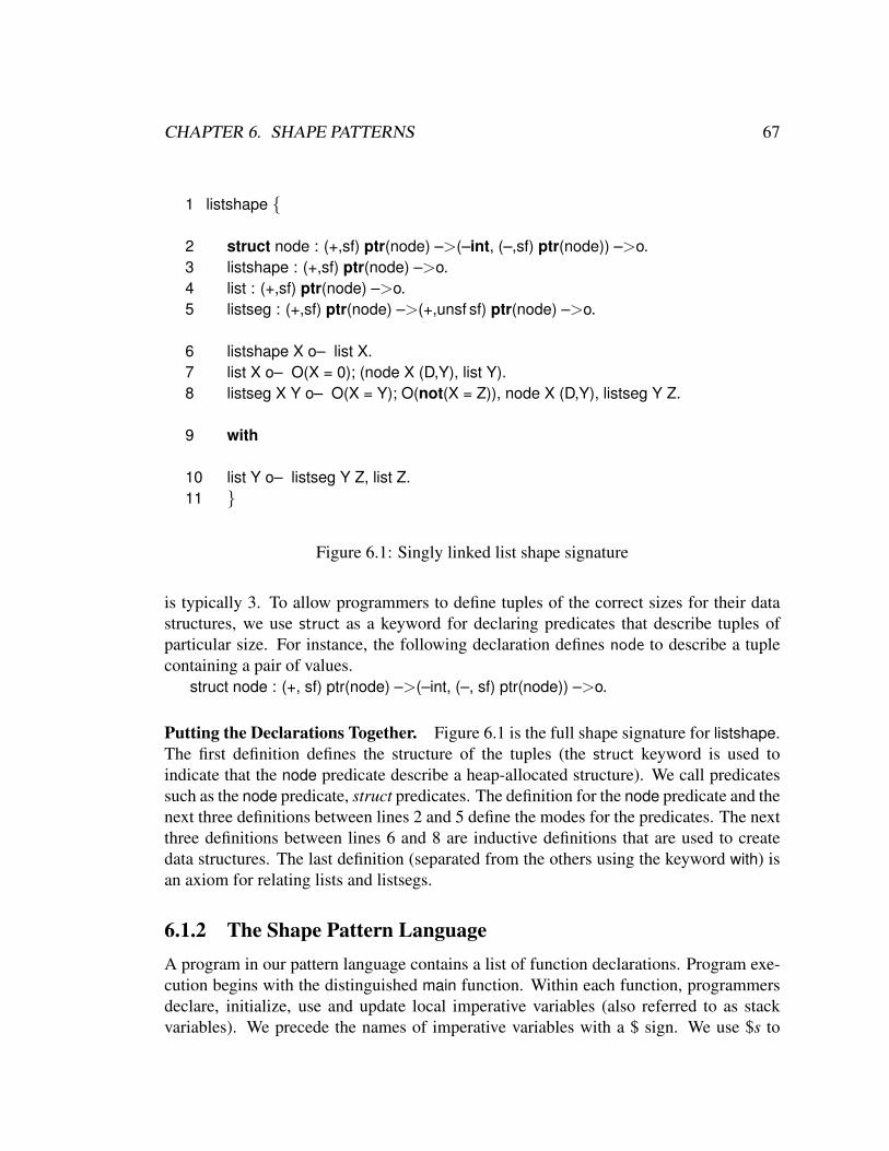
CHAPTER 6. SHAPE PATTERNS 67
1 listshape
2 struct node : (+,sf) ptr(node) –>(–int, (–,sf) ptr(node)) –>o.3 listshape : (+,sf) ptr(node) –>o.4 list : (+,sf) ptr(node) –>o.5 listseg : (+,sf) ptr(node) –>(+,unsf sf) ptr(node) –>o.
6 listshape X o– list X.7 list X o– O(X = 0); (node X (D,Y), list Y).8 listseg X Y o– O(X = Y); O(not(X = Z)), node X (D,Y), listseg Y Z.
9 with
10 list Y o– listseg Y Z, list Z.11
Figure 6.1: Singly linked list shape signature
is typically 3. To allow programmers to define tuples of the correct sizes for their datastructures, we use struct as a keyword for declaring predicates that describe tuples ofparticular size. For instance, the following declaration defines node to describe a tuplecontaining a pair of values.
struct node : (+, sf) ptr(node) –>(–int, (–, sf) ptr(node)) –>o.
Putting the Declarations Together. Figure 6.1 is the full shape signature for listshape.The first definition defines the structure of the tuples (the struct keyword is used toindicate that the node predicate describe a heap-allocated structure). We call predicatessuch as the node predicate, struct predicates. The definition for the node predicate and thenext three definitions between lines 2 and 5 define the modes for the predicates. The nextthree definitions between lines 6 and 8 are inductive definitions that are used to createdata structures. The last definition (separated from the others using the keyword with) isan axiom for relating lists and listsegs.
6.1.2 The Shape Pattern LanguageA program in our pattern language contains a list of function declarations. Program exe-cution begins with the distinguished main function. Within each function, programmersdeclare, initialize, use and update local imperative variables (also referred to as stackvariables). We precede the names of imperative variables with a $ sign. We use $s to

CHAPTER 6. SHAPE PATTERNS 68
range over shape variables and $x to range over integer or pointer variables. Each variableis given a basic type, which may be an integer type, a shape type, or a pointer type. Theshape types, such as listshape, are names of the shape signatures. The pointer types, suchas ptr(node), specify the kind of tuple a location points to.
Programmers create data structures by specifying the shapes they want in ILC. Theselogical formulas are interpreted as algorithms that allocate and initialize data structuresdesired by the programmer. To dereference data, programmers write pattern-matchingstatements, somewhat reminiscent of ML-style case statements, but in which the patternsare again logical formulas. Another algorithm matches the pattern against the currentheap; in other words, this algorithm checks whether the current heap can be described bythe logical formula. To update data structures, programmers simply specify the structureand contents of the new data structures they desire using logical formulas. The run-timesystem reuses heap space and updates the contents of existing data structures based onthe formulas. Finally, a free command allows programmers to deallocate data structuresas they would in an imperative language like C.
For the rest of this section we will demonstrate concretely how to construct anddeconstruct data structures using logical formulas by examples.
Creating Shapes. Programmers create data structures using the shape assignment state-ment as shown below.
$s : listshape := a1,a2,a3[root a1,node a1 (3, a2),node a2 (5, a3),node a3 (7, 0)]
The right-hand side of a shape assignment describes the shape to be created and theleft-hand side specifies the imperative shape variable to be assigned to. In this case,we will assume the shape variable $s has type listshape (see Figure 6.1). Variables a1,a2, and a3 in the braces are logical variables. Notice that they are different from theimperative variables, which always begin with $. Each of the logical variables representsthe starting address of a new tuple to be allocated on the heap. The formula in bracketsdescribes a heaplet that has the shape listshape. The special root predicate indicates thestarting address of this shape and must appear in all shape descriptions.
When we evaluate this shape assignment statement, we first allocate a new tuple foreach logical variable in the braces. The size of each tuple is determined by examiningthe type declaration of the node predicate in the listshape signature. Each variable issubsequently bound to the address of the corresponding tuple. Once the new nodes havebeen allocated, the integer data fields are initialized with the values that appear in theshape description. Finally, the location specified by the root predicate is stored into theshape variable $s.
The shape assignment statement above will create a singly linked list of length 3,which looks exactly like the one shown in Figure 3.1.
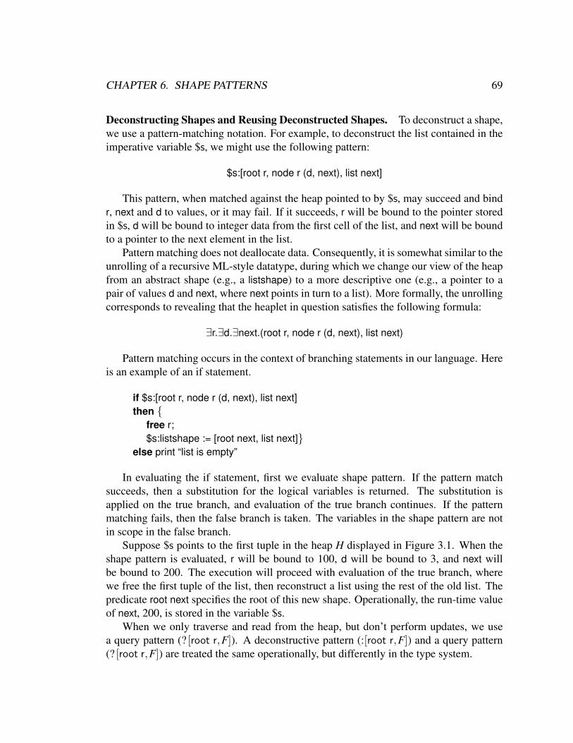
CHAPTER 6. SHAPE PATTERNS 69
Deconstructing Shapes and Reusing Deconstructed Shapes. To deconstruct a shape,we use a pattern-matching notation. For example, to deconstruct the list contained in theimperative variable $s, we might use the following pattern:
$s:[root r, node r (d, next), list next]
This pattern, when matched against the heap pointed to by $s, may succeed and bindr, next and d to values, or it may fail. If it succeeds, r will be bound to the pointer storedin $s, d will be bound to integer data from the first cell of the list, and next will be boundto a pointer to the next element in the list.
Pattern matching does not deallocate data. Consequently, it is somewhat similar to theunrolling of a recursive ML-style datatype, during which we change our view of the heapfrom an abstract shape (e.g., a listshape) to a more descriptive one (e.g., a pointer to apair of values d and next, where next points in turn to a list). More formally, the unrollingcorresponds to revealing that the heaplet in question satisfies the following formula:
∃r.∃d.∃next.(root r, node r (d, next), list next)
Pattern matching occurs in the context of branching statements in our language. Hereis an example of an if statement.
if $s:[root r, node r (d, next), list next]then
free r;$s:listshape := [root next, list next]
else print “list is empty”
In evaluating the if statement, first we evaluate shape pattern. If the pattern matchsucceeds, then a substitution for the logical variables is returned. The substitution isapplied on the true branch, and evaluation of the true branch continues. If the patternmatching fails, then the false branch is taken. The variables in the shape pattern are notin scope in the false branch.
Suppose $s points to the first tuple in the heap H displayed in Figure 3.1. When theshape pattern is evaluated, r will be bound to 100, d will be bound to 3, and next willbe bound to 200. The execution will proceed with evaluation of the true branch, wherewe free the first tuple of the list, then reconstruct a list using the rest of the old list. Thepredicate root next specifies the root of this new shape. Operationally, the run-time valueof next, 200, is stored in the variable $s.
When we only traverse and read from the heap, but don’t perform updates, we usea query pattern (? [root r,F]). A deconstructive pattern (:[root r,F]) and a query pattern(? [root r,F]) are treated the same operationally, but differently in the type system.
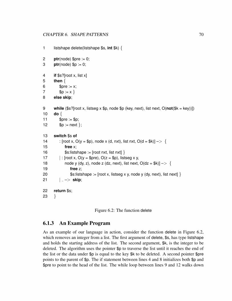
CHAPTER 6. SHAPE PATTERNS 70
1 listshape delete(listshape $s, int $k)
2 ptr(node) $pre := 0;3 ptr(node) $p := 0;
4 if $s?[root x, list x]5 then 6 $pre := x;7 $p := x 8 else skip;
9 while ($s?[root x, listseg x $p, node $p (key, next), list next, O(not($k = key))])10 do 11 $pre := $p;12 $p := next ;
13 switch $s of14 : [root x, O(y = $p), node x (d, nxt), list nxt, O(d = $k)] –> 15 free x;16 $s:listshape := [root nxt, list nxt] 17 | : [root x, O(y = $pre), O(z = $p), listseg x y,18 node y (dy, z), node z (dz, next), list next, O(dz = $k)] –> 19 free z;20 $s:listshape := [root x, listseg x y, node y (dy, next), list next] 21 | –> skip;
22 return $s;23
Figure 6.2: The function delete
6.1.3 An Example ProgramAs an example of our language in action, consider the function delete in Figure 6.2,which removes an integer from a list. The first argument of delete, $s, has type listshapeand holds the starting address of the list. The second argument, $k, is the integer to bedeleted. The algorithm uses the pointer $p to traverse the list until it reaches the end ofthe list or the data under $p is equal to the key $k to be deleted. A second pointer $prepoints to the parent of $p. The if statement between lines 4 and 8 initializes both $p and$pre to point to the head of the list. The while loop between lines 9 and 12 walks down
CHAPTER 6. SHAPE PATTERNS 71
the list maintaining the invariant expressed in the while condition through each iterationof the loop. This invariant states that (1) the initial part of the list is a listseg ending withthe pointer $p, (2) $p points to a node that contains a key and a next pointer, (3) the nextpointer itself points to a list, and (4) key is not the key of the current node. When eithercondition (2) or (4) is false, control breaks out of the loop (conditions (1) and (3) cannotbe falsified). The switch statement between lines 13 and 21 deletes node from the list (ifa node has been found). The first branch in the switch statement covers the case whenthe node to be deleted is the head of the list; the second branch covers the case when thenode to be deleted is pointed to by $p; the last (default) branch covers the case when $kis not present in the list.
6.1.4 What Could Go WrongAdopting a low-level view of the heap and using logic to describe recursive data structuresgives our language tremendous expressive power. However, the expressiveness calls foran equally powerful type system to ensure the memory safety of our language. We havealready mentioned some of the elements of this type system, including mode checkingfor logical declarations, and the use of inductive definitions and axioms to prove thatdata structures have the appropriate shapes. In this section, we summarize several keyproperties of the programming language’s overall type system: what could go wrong ifthese properties are missing, and what mechanisms we use to provide the appropriateguarantees. We will discuss these properties in more detail when we introduce the typesystem for our pattern language.
Safety of Deallocation. Uncontrolled deallocation can lead to double freeing and deref-erencing dangling pointers. We must make sure programmers do not use the deallocationcommand too soon or too often. To provide this guarantee, our linear type systemkeeps track of and describes (via logical formulas) the accessible heap, in much thesame way as we did earlier in this thesis (Section 3). In all cases, linearity constraintsseparate the description of one data structure from another to make sure that the effect ofdeconstruction and reconstruction of shapes is accurately represented.
Safety of Dereferencing Pointers. Pointers are dereferenced when a shape pattern-matching statement is evaluated. The algorithm could potentially dereference danglingpointers by querying ill-formed shape formulas. Consider the following pattern:
$s: [root r, node 12 (d, 0), node r (dr, 12)]Here there is no reason to believe “12” is a valid pointer. Predicate mode and type
checking prevents programmers from writing such ill-formed statements. To ensurethat algorithms for construction, inspection and deconstruction of heap values are well-defined and memory-safe, we analyze the programmer’s logical specifications using amode analysis inspired by similar analysis used in logic programs. This mode analysis is

CHAPTER 6. SHAPE PATTERNS 72
incorporated into a broader type system to ensure the safety of the overall programminglanguage.
Termination for Heap Shape Pattern Matching As we saw in the examples, duringthe execution of a program, the pattern-matching procedure is invoked to check if thecurrent program heap satisfies certain shape formulas. It is crucial to have a tractableand efficient algorithm for the pattern-matching procedure. In our system, this pattern-matching procedure is generated from the inductive definitions in the shape signature,and uses a bottom-up, depth-first algorithm. However, if the programmer defines apredicate Q as Q X o− Q X, then the decision procedure will never terminate. Toguarantee termination, we place a well-formedness restriction on the inductive definitionsthat ensures a linear resource is consumed before the decision procedure calls itselfrecursively. Our restriction rules out the bad definition of Q and others like it.
6.1.5 Three CaveatsFor the system as a whole to function properly, programmers are required to check thefollowing three properties themselves. Developing tools that could automatically checkthese properties are left for future work.
Closed Shapes. A closed shape is a shape from which no dangling pointers are reach-able. For example, lists, queues and trees are all closed shapes. On the other hand,the listseg definition presented earlier is not closed—if one traverses a heaplet describedby a listseg, the traversal may end at a dangling pointer. Shape signatures may containinductive definitions like listseg, but the top-level shape they define must be closed. Ifit is, then all data structures assigned to shape variables $s will also be closed and allpattern-matching operations will operate over closed shapes. This additional invariant isrequired to ensure shape pattern matching does not dereference dangling pointers.
Soundness of Axioms. For our proof system to be sound with regard to the memorysemantics, the programmer-defined axioms must be sound with respect to the semanticsgenerated from the inductive definitions. As in separation logic, checking properties ofdifferent data structures requires different axioms, and programmers must satisfy them-selves of the soundness of the axioms they write down and use. We have proven thesoundness of all the axioms that appear in this thesis (and axioms relating to other shapesnot in this thesis).
Uniqueness of Shape Matching. Given any program heap and a shape predicate witha known root location, at most one heaplet should match the predicate. For example,given the heap H in Figure 3.1, predicate list 200 describes exactly the portion of H that is

CHAPTER 6. SHAPE PATTERNS 73
reachable from location 200, ending in NULL (H2]H3). On the other hand, the predicatelistseg 100 X does not describe a unique shape on the heap H. The logic variable X canbe unified with 100, in which case the predicate listseg 100 X describes the empty heap;200, in which case the predicate listseg 100 X describes the heap H1; and 0, in which casethe predicate listseg 100 X describes the heap H. Without this property, the operationalsemantics would be nondeterministic. Programmers must verify this property themselvesby hand. Once again, it holds for all shapes described in this thesis.
These requirements are not surprising. For instance, separation logic’s specializedaxioms concerning lists and trees must be verified by hand as well. The requirementconcerning uniqueness of shapes is very similar to the precise predicates used in thework on separation and information hiding [59].
The rest of this chapter is organized as follows: in Section 6.2, we explain the detailsof the algorithmic interpretations of the logical definitions for heap shapes and the modeanalysis for preventing illegal memory operations. In Section 6.3, we introduce theformal syntax, semantics, and the type system of the overall language. In Section 6.4,we illustrate the extent of the language’s expressive power by explaining how to defineadjacency list representation of graphs and how to program operations on data structuresin our pattern language.
6.2 Logical Shape SignaturesA shape signature contains definitions that can be used to automatically generate a proofsystem used in type checking and a shape pattern matching decision procedure used atrun time. In the following subsections we define shape signatures rigorously, and explaineach of the components generated from shape signatures.
6.2.1 SyntaxThe syntax of the shape signatures is shown in Figure 6.3. We have seen most of thisnotation in the previous chapters. Again, we use the overbar notation x to denote a vectorof objects x. We use Ps to range over all the struct predicates such as node, P to rangeover user-defined predicates such as list. A literal L can be either an arithmetic formulaor a struct predicate or a user-defined predicate. We use F to range over formulas whichare either 1 (the empty heap) or the conjunction of a literal and another formula.
The head of a clause is a user-defined predicate and the body is a formula. For the easeof type checking, we gather the bodies of the same predicate into one definition I. Thenotation F means the additive disjunction of all the Fi in F. Axioms are also clauses.Notice that we use a more restrictive form for defining clauses than in the previous
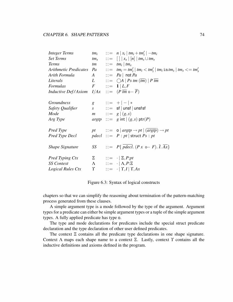
CHAPTER 6. SHAPE PATTERNS 74
Integer Terms tmi : := n | xi | tmi + tm′i | −tmi
Set Terms tms : := [ ] | xs | [n] | tms∪ tmsTerms tm : := tmi | tmsArithmetic Predicates Pa : := tmi = tm′
i | tmi < tm′i | tmiin tms | tms <= tm′
sArith Formula A : := Pa | not PaLiterals L : := ©A | Ps tm (tm) | P tmFormulas F : := 1 | L,FInductive Def / Axiom I/Ax : := (P tm o− F)
Groundness g : := + | − | ∗Safety Qualifier s : := sf | unsf | unsfsfMode m : := g | (g,s)Arg Type argtp : := g int | (g,s) ptr(P)
Pred Type pt : := o | argtp→ pt | (argtp)→ ptPred Type Decl pdecl : := P : pt | struct Ps : pt
Shape Signature SS : := P pdecl. (P x o− F). I. Ax
Pred Typing Ctx Ξ : := · | Ξ,P:ptSS Context Λ : := · | Λ,P:ΞLogical Rules Ctx ϒ : := · | ϒ, I | ϒ,Ax
Figure 6.3: Syntax of logical constructs
chapters so that we can simplify the reasoning about termination of the pattern-matchingprocess generated from these clauses.
A simple argument type is a mode followed by the type of the argument. Argumenttypes for a predicate can either be simple argument types or a tuple of the simple argumenttypes. A fully applied predicate has type o.
The type and mode declarations for predicates include the special struct predicatedeclaration and the type declaration of other user defined predicates.
The context Ξ contains all the predicate type declarations in one shape signature.Context Λ maps each shape name to a context Ξ. Lastly, context ϒ contains all theinductive definitions and axioms defined in the program.

CHAPTER 6. SHAPE PATTERNS 75
6.2.2 Semantics, Shape Pattern Matching and Logical DeductionThe shape signatures specify the semantics of the shapes, and the logical deductionsystem for proving properties about these shapes.
Store semantics. Let ϒ be the set of inductive definitions in the shape signatures. Wewrite H ϒ F to mean that heap H can be described by formula F, under the inductivedefinitions in ϒ. The semantics of logical formulas in the presence of inductive definitionsis the same as the one we defined in Section 3.2.2.
Shape Pattern-matching algorithm The shape pattern-matching algorithm determinesat run time if a given program heap satisfies a formula. We write MP(H;S;F;σ) to denotethe pattern-matching decision procedure. It takes four arguments: the heap H, a set oflocations S, a formula F, and a substitution σ for a subset of the free variables in F.Because F is a linear formula, we need to keep track of the disjointness of parts of theheap to satisfy subformulas of F. We use argument S to keep track of portions of the heapthat have already been used in the matching process. S contains heap locations that are inthe domain of H, but are not usable in the pattern matching currently.
We implement MP using an algorithm similar to Prolog’s depth-first, bottom-up proofsearch strategy. When a user-defined predicate is queried, we try to match all the clausebodies defined for this predicate. In evaluating a clause body, we evaluate the formulasin the body in left-to-right order as they appear. MP either succeeds and returns asubstitution for all the free variables in F, and the locations used in proving F, or fails andreturns no. A complete list of the rules for pattern matching is in Figure 6.4. We can seehow to keep track of the linearity by examining the rule for the struct predicates. Whenwe match a struct predicate, we have to make sure that none of the locations in the tuplehas already been used. After we successfully match a tuple, we add its locations to S sothey cannot be used again.
Logical Deduction. Type checking requires logical reasoning about the shapes of user-defined data structures. The inductive definitions and axioms defined by the user areaxioms in this logical deduction system. The logical deduction rules are the same asthe ones defined in Section 3.2.3. Recall that the judgment has the form: Θ;Γ;∆ =⇒ F.Initially, Γ will be populated by the inductive definitions and axioms from the shapesignatures.
One of the key properties of the logical deduction system is its soundness. For thelogical deduction system used here to be sound, we require that the additional axiomsprovided by the programmers be sound as well. Programmers are required to check thesoundness of the axioms by themselves. We proved that our logical deduction system issound with respect to the semantics modulo the soundness of axioms.
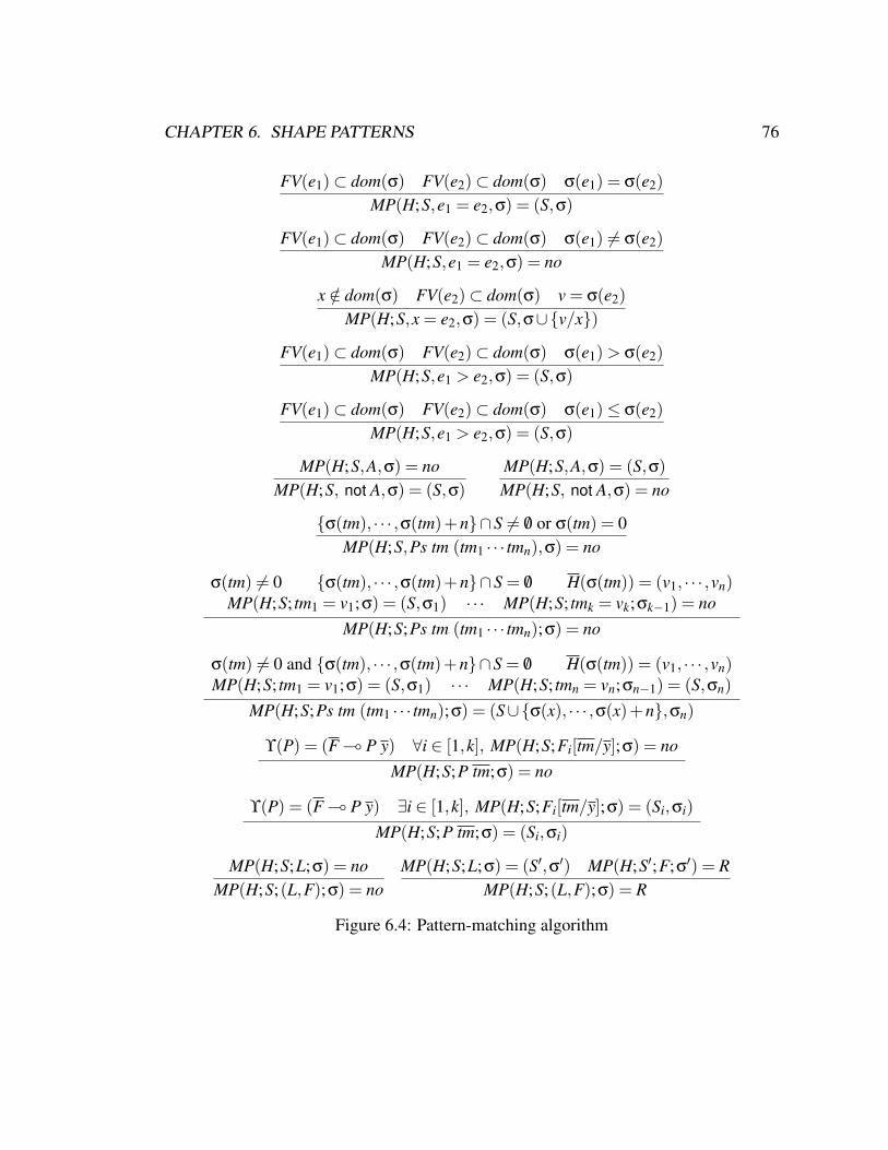
CHAPTER 6. SHAPE PATTERNS 76
FV(e1)⊂ dom(σ) FV(e2)⊂ dom(σ) σ(e1) = σ(e2)MP(H;S,e1 = e2,σ) = (S,σ)
FV(e1)⊂ dom(σ) FV(e2)⊂ dom(σ) σ(e1) 6= σ(e2)MP(H;S,e1 = e2,σ) = no
x /∈ dom(σ) FV(e2)⊂ dom(σ) v = σ(e2)MP(H;S,x = e2,σ) = (S,σ∪v/x)
FV(e1)⊂ dom(σ) FV(e2)⊂ dom(σ) σ(e1) > σ(e2)MP(H;S,e1 > e2,σ) = (S,σ)
FV(e1)⊂ dom(σ) FV(e2)⊂ dom(σ) σ(e1)≤ σ(e2)MP(H;S,e1 > e2,σ) = (S,σ)
MP(H;S,A,σ) = noMP(H;S, not A,σ) = (S,σ)
MP(H;S,A,σ) = (S,σ)MP(H;S, not A,σ) = no
σ(tm), · · · ,σ(tm)+n∩S 6= /0 or σ(tm) = 0MP(H;S,Ps tm (tm1 · · · tmn),σ) = no
σ(tm) 6= 0 σ(tm), · · · ,σ(tm)+n∩S = /0 H(σ(tm)) = (v1, · · · ,vn)MP(H;S; tm1 = v1;σ) = (S,σ1) · · · MP(H;S; tmk = vk;σk−1) = no
MP(H;S;Ps tm (tm1 · · · tmn);σ) = no
σ(tm) 6= 0 and σ(tm), · · · ,σ(tm)+n∩S = /0 H(σ(tm)) = (v1, · · · ,vn)MP(H;S; tm1 = v1;σ) = (S,σ1) · · · MP(H;S; tmn = vn;σn−1) = (S,σn)
MP(H;S;Ps tm (tm1 · · · tmn);σ) = (S∪σ(x), · · · ,σ(x)+n,σn)
ϒ(P) = (F ( P y) ∀i ∈ [1,k], MP(H;S;Fi[tm/y];σ) = noMP(H;S;P tm;σ) = no
ϒ(P) = (F ( P y) ∃i ∈ [1,k], MP(H;S;Fi[tm/y];σ) = (Si,σi)MP(H;S;P tm;σ) = (Si,σi)
MP(H;S;L;σ) = noMP(H;S;(L,F);σ) = no
MP(H;S;L;σ) = (S′,σ′) MP(H;S′;F;σ′) = RMP(H;S;(L,F);σ) = R
Figure 6.4: Pattern-matching algorithm
CHAPTER 6. SHAPE PATTERNS 77
Theorem 20 (Soundness of Logical Deduction)Assume the user-defined axioms (ϒA) are sound with respect to the store semanticsdefined by (ϒI), and ϒ = ϒI,ϒA and ·;ϒ;∆ =⇒ F, and σ is a grounding substitution forfree variables in the judgment, and H ϒI σ(∆), then H ϒI F.
Proof (sketch): By theorem 6, and theorem 7, and (ϒA) are sound with respect to thestore semantics defined by (ϒI).
6.2.3 Simple Type Checking for Shape SignaturesA simple type checking algorithm is devised to ensure that the arguments of the predicateshave the correct types according to the type declarations in the shape signature. Sincethe inductive definitions do not have type annotations, we need to infer the types of thearguments during type checking. There are two typing judgments, one is for checking thetype of terms, the other for checking the types of formulas. We use the context Ω to mapvariables to their types. The judgment Ω ` tm : (t,Ω′) means that the type of tm is t, andthe context Ω′ contains all type bindings for free variables in tm. Similarly, the judgmentΞ;Ω ` F : (o,Ω′) type checks F to have type o, and infers the types of free variables in Fwhich are collected into Ω′. Here context Ξ contains all the predicate type declarations.
We list the inference rules in Figure 6.5. We use Ω1∪Ω2 to denote the union of thetwo contexts if they agree on the types of the variables in the domains of both Ω1 and Ω2.Otherwise Ω1∪Ω2 is not defined. We use pti to denote the type of the ith argument of apredicate with type pt.
6.2.4 Mode AnalysisSimilar to simple type checking, mode analysis is also a compile-time check. Our modeanalysis serves two important purposes: (1) it ensures that the pattern-matching procedureknows the addresses of data structures it must traverse ( i.e., those addresses are groundwhen they need be), and (2) it ensures these addresses are safe to dereference. In thissection, we explain our mode analysis through a set of selected and simplified rules forthe analysis. There are two judgments in our mode analysis. The first judgment checksthe body of a definition in a context Π that maps variables to their safety modes s. Thissecond judgment has the form Ξ;Π ` F : Π′ and affirms that F is well-moded providedthat the variables in the domain of Π are ground (i.e., will be instantiated and availableat run time) and satisfy their associated safety mode. The output context Π′ contains thevariables that will be ground after the execution of F. The second, Ξ ` P x o− FOK,affirms that the inductive definition (P x o− F) is well-moded, satisfying both properties(1) and (2) above. Both judgments are parameterized by a function mode that maps eachuser-defined predicate P to its declared mode.
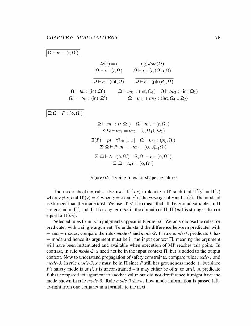
CHAPTER 6. SHAPE PATTERNS 78
Ω ` tm : (t,Ω′)
Ω(x) = tΩ ` x : (t,Ω)
x /∈ dom(Ω)Ω ` x : (t,(Ω,x:t))
Ω ` n : (int,Ω) Ω ` n : (ptr(P),Ω)
Ω ` tm : (int,Ω′)Ω ` −tm : (int,Ω′)
Ω ` tm1 : (int,Ω1) Ω ` tm2 : (int,Ω2)Ω ` tm1 + tm2 : (int,Ω1∪Ω2)
Ξ;Ω ` F : (o,Ω′)
Ω ` tm1 : (t,Ω1) Ω ` tm2 : (t,Ω2)Ξ;Ω ` tm1 = tm2 : (o,Ω1∪Ω2)
Ξ(P) = pt ∀i ∈ [1,n] Ω ` tmi : (pti,Ωi)Ξ;Ω ` P tm1 · · · tmn : (o,∪n
i=1Ωi)
Ξ;Ω ` L : (o,Ω′) Ξ;Ω′ ` F : (o,Ω′′)Ξ;Ω ` L;F : (o,Ω′′)
Figure 6.5: Typing rules for shape signatures
The mode checking rules also use Π∪(x:s) to denote a Π′ such that Π′(y) = Π(y)when y 6= x, and Π′(y) = s′ when y = x and s′ is the stronger of s and Π(x). The mode sfis stronger than the mode unsf. We use Π′ < Π to mean that all the ground variables in Π
are ground in Π′, and that for any term tm in the domain of Π, Π′(tm) is stronger than orequal to Π(tm).
Selected rules from both judgments appear in Figure 6.6. We only choose the rules forpredicates with a single argument. To understand the difference between predicates with+ and − modes, compare the rules mode-1 and mode-2. In rule mode-1, predicate P has+ mode and hence its argument must be in the input context Π, meaning the argumentwill have been instantiated and available when execution of MP reaches this point. Incontrast, in rule mode-2, x need not be in the input context Π, but is added to the outputcontext. Now to understand propagation of safety constraints, compare rules mode-1 andmode-3. In rule mode-3, x:s must be in Π since P still has groundness mode +, but sinceP’s safety mode is unsf, s is unconstrained – it may either be of sf or unsf. A predicateP that compared its argument to another value but did not dereference it might have themode shown in rule mode-3. Rule mode-5 shows how mode information is passed left-to-right from one conjunct in a formula to the next.

CHAPTER 6. SHAPE PATTERNS 79
Ξ;Π ` F : Π′
mode(Ξ,P) = (+,sf)→ ox:sf ∈Π
Ξ;Π ` P x : Πmode-1
mode(Ξ,P) = (+,unsf)→ ox:s ∈Π
Ξ;Π ` P x : Πmode-3
mode(Ξ,P) = (−,sf)→ oΞ;Π ` P x : Π∪(x:sf) mode-2
mode(Ξ,P) = (−,unsf)→ oΞ;Π ` P x : Π∪(x:unsf) mode-4
Ξ;Π ` L : Π′ Ξ;Π′ ` F : Π′′
Ξ;Π ` L,F : Π′′ mode-5
Ξ ` P x o− FOK
mode(Ξ,P) = (+,sf)→ oΞ;x:sf ` F : (x:sf),Π
Ξ ` P x o- F : OKmode-6
mode(Ξ,P) = (+,unsf)→ oΞ;x:unsf ` F : (x:s),Π
Ξ ` P x o- F : OKmode-7
mode(Ξ,P) = (+,unsfsf)→ o Ξ;x:unsf ` F : (x:sf),ΠΞ ` P x o- F : OK
mode-8
mode(Ξ,P) = (−,sf)→ oΞ; · ` F : (x:sf),Π
Ξ ` P x o- F : OKmode-9
mode(Ξ,P) = (−,unsf)→ oΞ; · ` F : (x:s),Π
Ξ ` P x o- F : OKmode-10
Figure 6.6: Selected and simplified mode analysis rules
To check that an inductive definition is well-moded, we need to check that the ar-guments in the head of the definition have the desired modes for safely and efficientlyevaluating the body of the definition, and that the predicates in the body of the definitionprovide arguments with the right modes after evaluation of the the body. For example,in mode-9, the argument of P should be ground and safe after evaluation of the body.Therefore, we check the body F with an empty Π context, and specify that after evaluationof F, x should be safe in the Π′ context.
Other mode analysis rules including rules that check built-in predicates and predicateswith multiple arguments are shown in Figure 6.7. The first argument of the built-inpredicate x = y is always an output and the second argument is an input. The mode-eq1rule is used when both of the arguments are integers. Since the second argument is aninput, we check that all the free variables in tm2 are in the Π context (tm2 is ground beforeevaluation). The Π′ context contains the free variable of tm1, since tm1 is unified withtm2 and is ground after execution.

CHAPTER 6. SHAPE PATTERNS 80
FV(tm2)⊂Π
Ξ;Π ` tm1 = tm2 : Π∪FV(tm1)mode-eq1
Π(tm2) = s tm1 /∈ dom(Π)Ξ;Π ` tm1 = tm2 : Π∪(tm1,s)
mode-eq2
Π(tm1) = s1 Π(tm2) = s2 s = max(s1,s2)Ξ;Π ` tm1 = tm2 : (o,Π∪(tm1,s)∪(tm2,s))
mode-eq3
mode(Ξ,P) = pm∀i ∈ [1,n] such that pmi = + FV(tmi)⊆ dom(Π)∀i ∈ [1,n] such that pmi = (+,unsf) or (+unsfsf) Π(tmi) = s∀i ∈ [1,n] such that pmi = (+,sf) Π(tmi) = sfΠ′ = Π∪x |pmi =−, and x ∈ FV(tmi)
∪tmi:s |pmi = (−,s)∪tmi:sf |pmi = (+,unsfsf)Ξ;Π ` Ptm1 · · · tmn : Π′ mode-p
mode(Ξ,P) = pmΠ = x j|pm j = +∪(x j,s)|pm j = (+,sin)
∪(x j,unsf)|pm j = (+,unsfsf)Ξ;Π ` P x : Π′ ∀i ∈ [1,n],Π ` Fi : Π′′ Π′′ < Π′
Ξ ` ((F1; · · · ;Fn) ( P x) OKmode-I
Figure 6.7: General mode analysis rule for inductive definitions
When both of the arguments have pointer types, we need to consider the safetyproperties of these arguments as well. The mode-eq2 rule is applied when tm1 is notin the Π context. We check that tm2 is ground, and we add tm1 to have the same safetyproperty as tm2 into the Π′ context. The mode-eq3 rule is used when tm1 is already in theΠ context. In this case, the safety property of tm1 and tm2 should both be updated to thestronger of the two.
The rule mode-p is the mode checking rule for a predicate that takes multiple argu-ments. This rule first checks that the Π context maps each input argument to its propersafety property. Secondly, the Π′ context collects the output arguments with their propersafety properties.
The rule mode-I checks the well-modedness of inductive definitions. It is the gener-alization of rules from mode-6 to mode-10.
CHAPTER 6. SHAPE PATTERNS 81
6.2.5 Requirements for Shape SignaturesIn Section 6.1.5, we made three requirements that have to be satisfied by the user-definedshapes signatures. We have informally discussed the importance of these requirements forthe type safety of our language. Now we give the formal definitions of these requirements,so that we can refer to them in proving properties of the pattern-matching decisionprocedure.
Closed ShapeP describes a closed shape, if for all H such that H P(l), H = H1] ·· ·]Hk, andfor all i ∈ [1,k], there exists v, v1, · · ·, vn such that Hi Ps v (v1, · · · ,vn), and ∀pti =m ptr(P), vi = 0 or vi ∈ ¯dom(H), where Λ(P) = Ξ, Ξ(Ps) = pt, n = size(P,Ps)
Soundness of Axioms ϒA is sound with regard to ϒI if for all Ax ∈ ϒA, /0 ϒI Ax.
Uniqueness of Shape MatchingIf Ξ;Π ` L : Π′, ∀x ∈ dom(Π) implies x ∈ dom(σ), and H1 σ1(L), H2 σ2(L),σ⊆ σ1, σ⊆ σ2, H1 ⊂ H, and H2 ⊂ H, then H1 = H2 and σ1 = σ2.
6.2.6 Correctness and Memory-safety of Matching ProcedureThe run-time behavior of the pattern matching decision procedure plays an importantrole in ensuring the termination and safety of the operational semantics of our patternlanguage. In this section, we prove formally that the pattern matching algorithm willalways terminate, provide correct answers, and be memory-safe.
Termination. In order for MP to terminate, we require that some linear resources beconsumed when we evaluate the clause body so that the usable heap gets smaller whenwe call MP on the user-defined predicates in the body. More specifically, in the inductivedefinitions for predicate P, there has to be at least one clause body that contains onlyarithmetic formulas and struct predicates. For clauses whose body contains user-definedpredicates, there has to be at least one struct predicate that precedes the first user-definedpredicate in the body. We statically check that these restrictions are met at compile time.
We proved the following theorem stating that MP terminates if the inductive defi-nitions are well-formed. We now use the judgment ` I OK to mean that I is not onlywell-moded, but also complies with the termination constraints.
Theorem 21 (Termination of MP)If for all I ∈ ϒ, ` I OK, then MPϒ(H;S;F;σ) always terminates.
Proof (sketch): By induction on the size of F, and Lemma 49 in Appendix D.
CHAPTER 6. SHAPE PATTERNS 82
Correctness. The following theorem states that the pattern-matching decision proce-dure always returns the correct result. The proof of Theorem 22 can be found in Ap-pendix D.
Theorem 22 (Correctness of MP)If Ξ;Π ` F : Π′, ∀x ∈ dom(Π), x ∈ dom(σ), and S ⊆ dom(H) then
• either MP(H;S;F;σ) = (S′,σ′), S′ ⊆ dom(H), σ⊆ σ′, and H′ σ′(F),where dom(H′) = (S′−S), and ∀x ∈ dom(Π′), x ∈ dom(σ′),
• or MP(H;S;F;σ) = no, and there does not exist a heap H′ which is the subheap ofH minus the locations in the set S, or σ′ such that σ⊆ σ′, and H′ σ′(F)
Proof (sketch): By induction on the depth of the derivation of the pattern matchingalgorithm.
Safety. Finally, we have proven that the MP procedure is memory safe.We use the following definition in stating our safety theorem. We say a term tm is
well-moded with respect to contexts Π, σ, and heap H, if tm is in the domain of Π, thenall the free variables in tm are in the domain of σ, and if Π(tm) = sf then σ(tm) is a validpointer on the heap H.
Because the program heap often contains many data structures, in our safety theorem(Theorem 23), we state that MP is memory safe on a larger heap than the one containingexactly the one shape MP is matching. Intuitively, MP is memory safe because it onlyfollows pointers reachable from the root of a “closed shape”. The proof of Theorem 23can be found in Appendix D.
Theorem 23 (Safety of MP)If ∀I ∈ ϒ, ` I OK, P is a closed shape, H1 P(l), Ξ;Π ` F : Π′, and ∀tm ∈ dom(Π), tmis well-moded with respect to Π, σ and H1 then
• either MP(H1]H2;S;F;σ) = (S′,σ′), and MP is memory safe, and ∀tm∈ dom(Π′),tm is well-moded with respect to Π′, σ′ and H1.
• or MP(H1]H2;S;F;σ) = no, and MP is memory safe.
Proof (sketch): By induction on the structure of the formula to be matched.

CHAPTER 6. SHAPE PATTERNS 83
Basic Types t : := int | ptr(P)Regular Types τ : := t | PFun Types τ f : := (τ1×·· ·× τn)→ P
Vars var : := $x | xExprs e : := var | n | e+ e | −eArgs arg : := e | $sShape Forms shp : := root v,FShape Patterns pat : := : [shp] | ?[shp]Atoms a : := ©A | $s patConj Clauses cc : := a | cc,cc
Branch b : := ( pat→ s)Branches bs : := b | b ′|′ bsStatements s : := skip | s1 ; s2 | $x := e
| if cc then s1 else s2 | while cc do s| switch $s of bs | $s := x [shp]| free v | $s := f ( arg )
Fun Bodies fb : := s1 ; fb | return $s
Local Decl ldecl : := t $x := v | P $sFun Decl fdecl : := P f (x1 : τ1, · · ·xn : τn) ldecl; fb
Program prog : := SS; fdecl
Values v : := x | n | $s
Figure 6.8: Syntax of the language constructs
6.3 The Programming LanguageAfter defining various data structures in the shape signatures, programmers can use thosedefinitions to program operations on the data structures. In this section, we explain howto embed the mode analysis and the proof system into the type system, and, likewise,the pattern-matching algorithm into the operational semantics, and thereby integrate theverification technique into the language.

CHAPTER 6. SHAPE PATTERNS 84
6.3.1 SyntaxA summary of the syntax of our pattern language is shown in Figure 6.8. The basic typesare the integer type and the pointer type. Functions take a tuple of arguments and alwaysreturn a shape type.
We use x to range over logical variables in formulas, $x to range over stack variables,and $s to range over shape variables. Shape variables live on the stack and store thestarting address of data structures allocated on the heap. We use e to denote expressionsand arg to denote function arguments, which can be either expressions or shape variables.Shape formulas shp are the multiplicative conjunction of a set of predicates. We use aspecial root predicate to indicate the starting address of the shape. The first predicatein a shape formula is always the root predicate. A shape pattern pat can be either aquery pattern (? [shp]) or a deconstructive pattern (:[shp]). The conditional expressionsin if statements and while loops make use of conjunctive clauses cc that describes theshape patterns of one or more disjoint data structures. The conjunctive clause cc is themultiplicative conjunction of atoms a, which can be either arithmetic formulas ©A orshape patterns ($s pat).
The statements in our language include skip, statement sequences, expression assign-ments, branching statements, shape assignments, deallocation, and function calls.
A function body is a statement followed by a return instruction. A program consistsof shape signatures and a list of function declarations. Lastly, the values in our languageare integers, variables, and shape variables.
6.3.2 Operational SemanticsIn this section, we formally define the operational semantics of our pattern language.
Runtime Constructs. We define several run-time constructs to represent the machinestate during execution of a program. There are two run-time statements: fail and halt.Statement fail signals the failure in matching any of the branches in a switch statement.Statement halt signals the termination of the execution of the entire program. We de-fine evaluation contexts to specify the evaluation order. The hole in the context is aplaceholder for the expression or statement currently being evaluated. The machine statecontains an environment E, which maps stack variables to their values, and a controlstack S, which is a stack of evaluation contexts waiting for the return of function calls.We use context Φ to map function names to their definitions. We write E($x) to denotethe value E maps $x to. We write E(F) to denote the formula resulting from substitutingfree stack variables in F with their values in E.

CHAPTER 6. SHAPE PATTERNS 85
Runtime stmt s : := fail | haltEval Ctxt Ce : := [ ]e | Ce + e | v+Ce | −Ce
Cstmt : := [ ]stmt | Cstmt ; s | $x := Ce| $s := f ( v1, · · ·vk,Ce,ek+2, · · · )
Environment E : := · | E,$x 7→ n | E,$s 7→ nEnv Stack Es : := • | E .EsControl Stack S : := • | (Cstmt ; fb)[$s := •].SCode Environment Φ : := · |Φ, f 7→ [x1, · · · ,xn] ldecls fb
Operational Semantics for Expressions. The evaluation of expressions relies only onthe current environment E, so the small-step relationship of expressions has the form(E;e) 7−→ e′. Below are the formal definitions.
(E;e) 7−→ E(e′)var (E;$x) 7−→ E($x)sum (E;v1 + v2) 7−→ v where v = v1 + v2ctx (E;Ce[e]) 7−→ Ce[e′] if (E;e) 7−→ e′
A stack variable evaluates to its mapping in the environment, the sum of two integersevaluates to their sum, and the rule ctx controls the evaluation order.
Operational Semantics for Statements The machine state for evaluating statementsother than the function call is a tuple (E;H;s). The environment E maps stack variablesto their values. H is the program heap, and s is the statement being evaluated. We write(E;H;s) 7−→ (E ′;H′;s′) to denote the small-step operational semantics for statements. Wepresent all the rules in Figure 6.9. Most of the rules are straightforward and we explain afew selected rules that use formulas to manipulate the heap.
To deallocate a tuple, programmers supply the free statement with the starting addressv of that tuple. The heaplet to be freed is easily identified, since the size of the tuple isstored in v.
The shape assignment statements allow programmers to create data structures. Duringthe execution of a shape assignment statement, the heap is updated according to the shapeformulas in the statement. In the end, the root of the new shape is stored in $s. The coreprocedure is CreateShape, which takes as its arguments the current heap, the shape nameP, and the shape formula. It returns the updated heap and the root of the new shape. Inorder to define this procedure, we define function size(F,x) to extract the appropriate sizeof the tuple x points to according to the shape formula F. For instance, if Ps x (3,0) isa subformula of F, then size(F,x) = 2. The CreateShape procedure first allocates on the

CHAPTER 6. SHAPE PATTERNS 86
(E;H;s) 7−→ (E ′;H′;s′)seq (E;H;(skip ; s)) 7−→ (E;H;s)
assign-exp (E;H;$x := v) 7−→ (E[$x := v];H;skip)free (E;H; free v) 7−→ (E;H1;skip) where H = H1]H2
and H2(v) = n, dom(H2) = v,v+1, · · · ,v+nassign-shape (E;H;$s:P := x [root (v),F]) 7−→ (E[$s := v′];H′;skip)
where (v′,H′) = CreateShape(H,P,x [root (v),F])CreateShape(H,P,x(root n,F)) = (H′,n[l/x])where1. ki = size(F,xi)2. (H1, l1) = alloc(H,k1), · · · ,(Hn, ln) = alloc(Hn−1,kn)3. F′ = F[l1 · · · ln/x1 · · ·xn]4. H′ = H[v+ i := vi] for all (Ps v (v1 · · ·vk)) ∈ F′
If-t (E;H; if cc then s1 else s2) 7−→ (E;H;σ(s1))if JccKE = (F,σ′) and MP(H;F; /0;σ′) = (SL;σ)
If-f (E;H; if cc then s1 else s2) 7−→ (E;H;s2)if JccKE = (F,σ) and MP(H;F; /0;σ) = no
while-t (E;H;while cc do s) 7−→ (E;H;(σ(s1) ; while x cc do s))if JccKE = (F,σ′) and MP(H;F; /0;σ′) = (SL;σ)
while-f (E;H;while cc do s) 7−→ (E;H;skip)if JccKE = (F,σ) and MP(H;F; /0;σ) = no
switch-t (E;H;switch $s of ([root (xi),F]→ sk)|bs )7−→ (E;H;σ(sk)) if MP(H;E(F); /0;E($s)/xi) = (SL;σ)
switch-f (E;H;switch $s of ([root (xi),F]→ sk) | bs )7−→ (E;H;switch x of bs ) if MP(H;E(F); /0;E($s)/xi) = no
fail (E;H;switch $s of ([root (xi),F]→ sk))7−→ (E;H; fail) if MP(H;E(F); /0;E($s)/xi) = no
ctxt-e (E;H;Cstmt [e]) 7−→ (E ′;H′;Cstmt [e′]) if (E;e) 7−→ e′
ctxt-fail (E;H;Cstmt [s]) 7−→ (E ′;H′; fail) if (E;H;s) 7−→ (E ′;H′; fail)ctxt-stmt (E;H;Cstmt [s]) 7−→ (E ′;H′;Cstmt [s′]) if (E;H;s) 7−→ (E ′;H′;s′)
Figure 6.9: Operational semantics for statements
heap a new tuple of the appropriate size for each variable in braces. The starting addressesof these new tuples are bound to the variables. Lastly, we update the contents of the heapaccording to the struct predicates in the formula.
When an if statement is evaluated, the pattern-matching procedure is called to checkif the conditional expression is true. If MP succeeds and returns a substitution σ forthe logical variables, we continue with the evaluation of the true branch with σ applied;otherwise, the false branch is evaluated. Notice that the conditional expression cc is not

CHAPTER 6. SHAPE PATTERNS 87
in the form of a logical formula; therefore, we need to convert cc to its equivalent formulaFcc before invoking the pattern-matching procedure MP. We define JccKE to extract Fccand a substitution σ for the logical variables from cc. Intuitively, Fcc is the conjunctionof all the shape formulas with run-time values substituted for the stack variables and theroot predicate dropped.
For example, if E($s) = 100 and cc is ($s : [root r, node r (d, next), list next]) then logicvariable r must be 100 as the clause specifies that r is the “root” the value of $s. Hence,the substitution σ is 100/r, and Fcc is (node r (d, next), list next). MP is called with thecurrent program heap, an empty set, the formula Fcc, and the substitution σ from JccKE .Below is the formal definition of JccKE = (F,σ).
J©AKE = (E(©A), ·)J$s?[root x,F]KE = (E(F),E($s)/x)J$s:[root x,F]KE = (E(F),E($s)/x)Jcc1,cc2 KE = ((F1,F2),σ1∪σ2) if Jcci KE = (Fi,σi)
The while loop is very similar to the if statement. If the conditional expression is truethen the loop body is evaluated and the loop will be re-entered; otherwise, the loop isexited.
The switch statement branches on a shape variable against a list of shape patterns.The shape patterns in switch statements are special cases of conditional expressions. Theshape variable being branched on is the only shape being considered. If matching on thecurrent shape pattern succeeds, the branch body is evaluated; otherwise the next branchis considered. If the pattern of the last branch failed, then the switch statement evaluatesto fail.
Operational Semantics for Function Bodies. The machine state for evaluating func-tion bodies makes use of a control stack S to remember the return point of each functioncall. We present the operational semantics for function bodies in Figure 6.10. Wedefine env(ldecls,E) to denote the environment for local variables in ldecls. Declarationsin ldecls may initialize variables using variables in the environment E. For example,env(t $x := $a,E) = $x 7→ E($a).
When a function call is evaluated, the current evaluation context is pushed ontothe control stack and the evaluation of the body of the callee starts. Upon return, theevaluation context of the caller is popped off the control stack, and the return value isplugged into the caller’s evaluation context.
6.3.3 Type SystemOur type system is a linear type system. The contexts in the typing judgments not onlykeep track of the types of the variables, but also describe the current status of programstate: what the valid shapes are, and what the structure of the accessible heap is. The

CHAPTER 6. SHAPE PATTERNS 88
(E;H;S; fb) 7−→ (E ′;H′;S′; fb′)fun-call (E;H;S;(Cstmt ; fb)[$s := f ( v1 . . .vn )])
7−→ (E f .E;H;(Cstmt ; fb)[$s := •].S; fb f )if Φ( f ) = ([x1 . . .xn]ldecls; fb f )Ea = x1 7→ E(v1), · · · ,xn 7→ E(vn) E f = Ea,env(ldecls,Ea)
fun-ret (E .Es;H;(Cstmt ; fb)[$s := •].S; return $s1)7−→ (Es[$s := E($s1)];H;S;(Cstmt ; fb)[skip])
halt (•;H;•; return v) 7−→ (•;H;•;halt)fail (E;H;S;(fail ; fb)) 7−→ (•;H;•;halt)skip (E;H;S;(skip ; fb)) 7−→ (E;H;S; fb)
context-stmt (E;H;S;(s ; fb)) 7−→ (E;H;S;(s′ ; fb)) if (E;H;s) 7−→ (E ′;H′;s′)
Figure 6.10: Operational semantics of function bodies
contexts used in the typing judgments are shown below.
Variable Ctx Ω : := · |Ω,var:tInitialized Stack Variable Ctx Γ : := · | Γ,$s:PUninitialized Shape Variable Ctx Θ : := · |Θ,$s:PHeap Ctx ∆ : := · | ∆,P tm1 · · · tmn | ∆,Ps tm (tm1, · · · , tmn)Code Ctx Ψ : := · |Ψ, f : (τ1×·· ·× τn)→ P
The context Ω maps variables to their types. Both Γ and Θ map shape variables totheir types. During type checking, Γ specifies the initialized shape variables, while Θ
specifies the uninitialized shape variables. Variables in Θ may not contain valid heappointers, but may be initialized later in the program. Context ∆ is a set of formulasthat describes the accessible portions of the heap. Contexts Γ and ∆ describe the entireprogram heap. For example, if Γ = $s:listshape and ∆ = node 400 (11, 0), and theenvironment is E = $s 7→ 100, then the current heap must satisfy the formula (listshape100, node 400 (11,0)). Context Ψ maps function names to their types.
The judgments in our type system are listed below.
Expression typing Ω `e e : tConjunctive clause typing Ω;Γ `cc cc : (Ω′;Γ′;Θ;∆)Conjunctive clause modes checking Γ;Π ` cc : Π′
Statement typing Ω;Γ;Θ;∆ ` s : (Γ′;Θ′;∆′)Function Body Typing Rules Ω;Γ;Θ;∆ ` fb : P
Each of these judgments is also implicitly indexed by the context for shape signaturesΛ, axioms ϒ, and function type bindings Ψ. We leave these contexts implicit as they areinvariant through the type checking process.
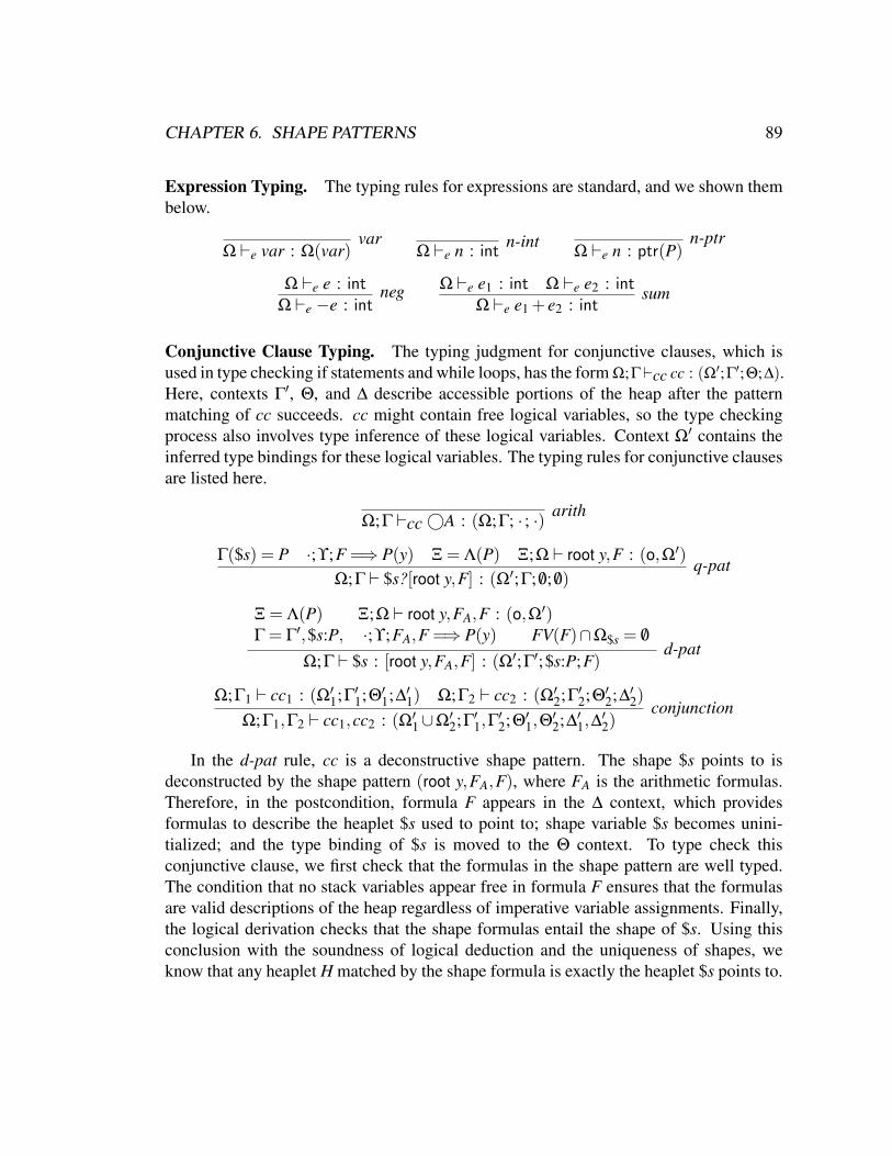
CHAPTER 6. SHAPE PATTERNS 89
Expression Typing. The typing rules for expressions are standard, and we shown thembelow.
Ω `e var : Ω(var)var
Ω `e n : intn-int
Ω `e n : ptr(P)n-ptr
Ω `e e : intΩ `e −e : int
neg Ω `e e1 : int Ω `e e2 : intΩ `e e1 + e2 : int
sum
Conjunctive Clause Typing. The typing judgment for conjunctive clauses, which isused in type checking if statements and while loops, has the form Ω;Γ`cc cc : (Ω′;Γ′;Θ;∆).Here, contexts Γ′, Θ, and ∆ describe accessible portions of the heap after the patternmatching of cc succeeds. cc might contain free logical variables, so the type checkingprocess also involves type inference of these logical variables. Context Ω′ contains theinferred type bindings for these logical variables. The typing rules for conjunctive clausesare listed here.
Ω;Γ `cc ©A : (Ω;Γ; · ; ·) arith
Γ($s) = P ·;ϒ;F =⇒ P(y) Ξ = Λ(P) Ξ;Ω ` root y,F : (o,Ω′)Ω;Γ ` $s?[root y,F] : (Ω′;Γ; /0; /0)
q-pat
Ξ = Λ(P) Ξ;Ω ` root y,FA,F : (o,Ω′)Γ = Γ′,$s:P, ·;ϒ;FA,F =⇒ P(y) FV(F)∩Ω$s = /0
Ω;Γ ` $s : [root y,FA,F] : (Ω′;Γ′;$s:P;F)d-pat
Ω;Γ1 ` cc1 : (Ω′1;Γ′1;Θ′
1;∆′1) Ω;Γ2 ` cc2 : (Ω′2;Γ′2;Θ′
2;∆′2)Ω;Γ1,Γ2 ` cc1,cc2 : (Ω′
1∪Ω′2;Γ′1,Γ
′2;Θ′
1,Θ′2;∆′1,∆
′2)
conjunction
In the d-pat rule, cc is a deconstructive shape pattern. The shape $s points to isdeconstructed by the shape pattern (root y,FA,F), where FA is the arithmetic formulas.Therefore, in the postcondition, formula F appears in the ∆ context, which providesformulas to describe the heaplet $s used to point to; shape variable $s becomes unini-tialized; and the type binding of $s is moved to the Θ context. To type check thisconjunctive clause, we first check that the formulas in the shape pattern are well typed.The condition that no stack variables appear free in formula F ensures that the formulasare valid descriptions of the heap regardless of imperative variable assignments. Finally,the logical derivation checks that the shape formulas entail the shape of $s. Using thisconclusion with the soundness of logical deduction and the uniqueness of shapes, weknow that any heaplet H matched by the shape formula is exactly the heaplet $s points to.

CHAPTER 6. SHAPE PATTERNS 90
Conjunctive Clause Mode Checking. At run time, the pattern matching decision pro-cedure is called to check if the current heap can be described by the conjunctive clausescc. To ensure the memory safety of the pattern matching procedure, we apply modeanalysis on cc. The mode checking rules for cc use the mode checking rules for formulasto check each shape pattern in cc in left-to-right order. We show the rules for modechecking the conjunctive clauses below.
·;Π ` A : Π′
Γ;Π `©A : Π′ arith-m
Γ($s) = P Ξ = Λ(P) Ξ;Π∪x:sf ` F : Π′
Γ;Π ` $s?[root x,F] : Π′ q-pat-m
Γ($s) = P Ξ = Λ(P) Ξ;Π∪x:sf ` F : Π′
Γ;Π ` $s:[root x,F] : Π′ d-pat-m
Γ;Π ` cc1 : Π′ Γ;Π′ ` cc2 : Π′′
Γ;Π ` cc1,cc2 : Π′′ conjunction-m
In the d-pat-m rule, since $s points to a valid shape, its root pointer is a valid pointer.Therefore, the argument x of the root predicate is a safe pointer argument. We mode checkthe formula in the shape pattern under the context, which is the union of the context Π
and the context specifying x is a safe pointer.
Statement Type Checking. The typing judgment for statements has the form Ω;Γ;Θ;∆
` s : (Γ′;Θ′;∆′). The contexts to the left of the turnstile describe the program state beforeexecuting s, and the contexts to the right of the turnstile describe the program state afterexecuting s. We present the typing rules for statements below.
Ω;Γ;Θ;∆ ` skip : (Γ;Θ;∆)skip
Ω;Γ;Θ;∆ ` s : (Γ′;Θ′;∆′) Ω;Γ′;Θ′;∆′ ` s′ : (Γ′′;Θ′′;∆′′)Ω;Γ;Θ;∆ ` s ; s′ : (Γ′′;Θ′′;∆′′)
seq
Ω;Γ ` cc : (Ω′,Γ′,Θ′,∆′) Π = ground(Ω) Γ;Π ` cc : Π′
Ω′;Γ′;Θ,Θ′;∆,∆′ ` s1 : (Γ′′;Θ′′;∆′′) Ω;Γ;Θ;∆ ` s2 : (Γ′′;Θ′′;∆′′)
Ω;Γ;Θ;∆ ` if cc then s1 else s2 : (Γ′′;Θ′′;∆′′)if
Ω;Γ ` cc : (Ω′,Γ′,Θ′,∆′) Π = ground(Ω) Γ;Π ` cc : Π′
Ω′;Γ′;Θ,Θ′;∆,∆′ ` s : (Γ;Θ;∆)Ω;Γ;Θ;∆ ` while cc do s : (Γ;Θ;∆) while

CHAPTER 6. SHAPE PATTERNS 91
Ω `e $x : t Ω `e e : tΩ;Γ;Θ;∆ ` $x := e : (Γ;Θ;∆)
assign-exp
Ξ = Λ(P) Ξ;Ω ` root v,F : (o,Ω′) ·;ϒ;F =⇒ P(v)∆x = Ps xi e |Ps xi e ∈ F ∆ = ∆′,∆′′ F = ∆x,∆F
∀P tm,P tm ∈ ∆′′ iff P tm ∈ ∆F ∀Ps tm e ∈ ∆′′ iff Ps tm e′ ∈ ∆F
Ω;Γ;Θ;∆ ` $s:P := x[root (v),F] : (Γ′,$s:P;(Θ\($s:P));∆′)assign-shape
For all i,1≤ i≤ n, Ω;Γ;Θ;∆ `$s b i : (Γ′;Θ′;∆′)Ω;Γ;Θ;∆ ` switch $s of bs : (Γ′;Θ′;∆′) switch
Γ($s) = P Ξ = Λ(P) Ξ;Ω ` root xi,F : (o,Ω′)Ξ;ground(Ω)∪xi:sf ` F : Π ∀xi ∈ dom(Ω′),xi ∈ dom(Π)
·;ϒ;F =⇒ P(xi) Ω′;Γ;Θ;∆ ` s : (Γ′;Θ′;∆′)Ω;Γ;Θ;∆ `$s ?[root (xi),F]→ s : (Γ′;Θ′;∆′)
pat-?
Γ = Γ′,$s:P Ξ = Λ(P) shp = root (xi),FA,FΞ;ground(Ω)∪xi:sf ` F : Π ∀xi ∈ dom(Ω′),xi ∈ dom(Π)
·;ϒ;FA,F =⇒ P(xi) Ξ;Ω ` root xi,F : (o,Ω′) FV(F)∩Ω$ = /0
Ω′;Γ′;Θ,$s:P;∆,F ` s : (Γ′′;Θ′;∆′)Ω;Γ;Θ;∆ `$s :[shp]→ s : (Γ′′;Θ′;∆′)
pat-:
Ω(v) = ptr(Ps) ∆ = (Ps v (e1 · · ·ek)),∆′
Ω;Γ;Θ;∆ ` free (v) : (Γ;Θ;∆′)free
Ψ( f ) = (τ1×·· ·× τn → P) Θn = Θ,$s:PΩ;Γ;Θ `a a1 : (τ1;Γ1;Θ1) · · · Ω;Γn−1;Θn−1 `a an : (τn;Γn;Θn)
Ω;Γ;Θ;∆ ` $s := f ( a1, · · · ,an ) : ((Γn,$s:P;Θ;∆)fun-call
The rule if first type checks the conjunctive clause cc. From type checking cc, weinfer the type bindings for the free logical variables. In addition, we also obtain theformulas describing the heap if cc is valid. We then type check the two branches of theif statement. The true branch is only taken when cc is proved to be true; hence, the truebranch is checked under the new contexts resulting from checking cc. On the other hand,the false branch is type checked under the contexts under which the if statement is typechecked. The end of the if statement is a program merge point, so the true and the falsebranch should lead to the same state.
Another important piece of type checking the if statement is the mode analysis ofcc. We need to make sure that the pattern-matching procedure will not access danglingpointers while matching cc against the program heap at run time.

CHAPTER 6. SHAPE PATTERNS 92
In the mode analysis, the Π context contains the groundness and safety informationof the arguments before cc is evaluated. It depends on the variable context Ω. We writeground(Ω) to denote the Π context derived from context Ω. It is defined as follows:
ground(Ω) = var |Ω(var) = int∪(var:unsf) |Ω(var) = ptr(P)
Before evaluating a statement, the run-time values should already have been substitutedfor the logical variables in the statement. Therefore, all the variables in Ω are groundbefore we evaluate cc. We have no information on the validity of pointer variables, sothey are considered unsafe.
A simple examination of the mode analysis rule tells us that since the only safepointers we assume before evaluating cc are the root pointers of valid shapes, the pattern-matching procedure is guaranteed to be memory safe. We sketch the proof of this inAppendix E, Lemma 57.
Type checking while loops is similar to checking the if statements. The contextsunder which the while loop is type checked are in effect loop invariants. The rule whilefirst type check the conjunctive clause. The loop body is checked against the contextsresulting from checking the conjunctive clauses. The contexts resulting from checkingthe loop body should be the same as the contexts under which the while loop is typechecked so that the loop can be re-entered.
The rule assign-shape first checks that the shape variable $s is uninitialized – thischeck prevents memory leaks. It does so by checking that $s belongs to Θ (not Γ). Thethird premise in the assignment rule checks that the shape formula entails the shape ofthe variable $s. The rest of the premises ensure that every piece of heap used during theshape assignment is accounted for. To be more precise, the union of the formulas used toconstruct this shape and the leftover formulas in ∆′ should be the same as the formulas in∆ plus the new heaplets allocated. The typing rule looks complicated because we allowmultiple updates to the heap during assignment. For example, if Ps l (5,0) is available,then we allow Ps l (10, 0) to be used in the shape assignment. This means that after theshape assignment, the heap cell that used to contain 5 now contains 10.
The typing rule for the switch statement, switch, requires that each branch results inthe same program state. Each branch in the switch statement can be viewed as a simplifiedif statement with only a true branch, and the conditional expression only considers theshape pattern for one data structure.
To ensure the memory safety of deallocation, the typing rule for the free statementchecks that the location to be freed is in the accessible portion of the heap. The typingrule also makes sure that the formula describing the heaplet to be freed is removed fromthe linear context of the postcondition of the free statement. The postcondition guaranteesthat this heaplet can never be accessed again after the free statement is executed, andprevents double freeing.
The rule fun-call first looks up the function type in the Ψ context. It then checksthe arguments against the specified argument types. When a shape variable is used as a
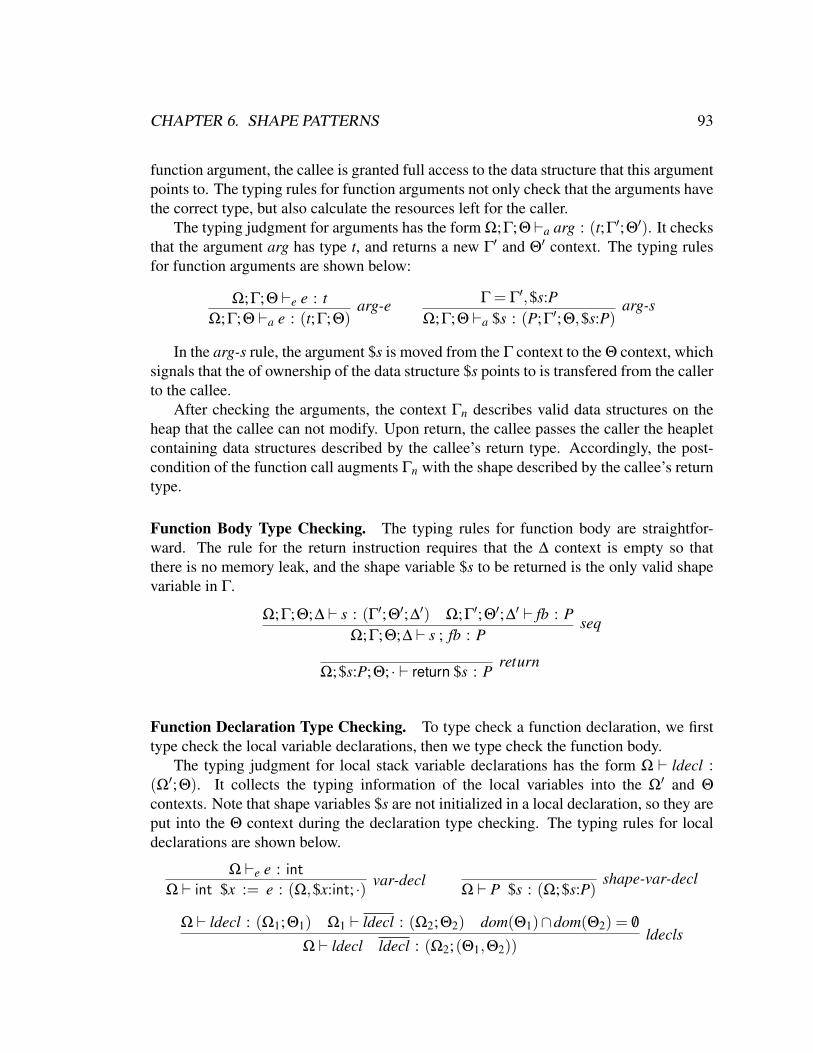
CHAPTER 6. SHAPE PATTERNS 93
function argument, the callee is granted full access to the data structure that this argumentpoints to. The typing rules for function arguments not only check that the arguments havethe correct type, but also calculate the resources left for the caller.
The typing judgment for arguments has the form Ω;Γ;Θ `a arg : (t;Γ′;Θ′). It checksthat the argument arg has type t, and returns a new Γ′ and Θ′ context. The typing rulesfor function arguments are shown below:
Ω;Γ;Θ `e e : tΩ;Γ;Θ `a e : (t;Γ;Θ)
arg-e Γ = Γ′,$s:PΩ;Γ;Θ `a $s : (P;Γ′;Θ,$s:P)
arg-s
In the arg-s rule, the argument $s is moved from the Γ context to the Θ context, whichsignals that the of ownership of the data structure $s points to is transfered from the callerto the callee.
After checking the arguments, the context Γn describes valid data structures on theheap that the callee can not modify. Upon return, the callee passes the caller the heapletcontaining data structures described by the callee’s return type. Accordingly, the post-condition of the function call augments Γn with the shape described by the callee’s returntype.
Function Body Type Checking. The typing rules for function body are straightfor-ward. The rule for the return instruction requires that the ∆ context is empty so thatthere is no memory leak, and the shape variable $s to be returned is the only valid shapevariable in Γ.
Ω;Γ;Θ;∆ ` s : (Γ′;Θ′;∆′) Ω;Γ′;Θ′;∆′ ` fb : PΩ;Γ;Θ;∆ ` s ; fb : P
seq
Ω;$s:P;Θ; · ` return $s : Preturn
Function Declaration Type Checking. To type check a function declaration, we firsttype check the local variable declarations, then we type check the function body.
The typing judgment for local stack variable declarations has the form Ω ` ldecl :(Ω′;Θ). It collects the typing information of the local variables into the Ω′ and Θ
contexts. Note that shape variables $s are not initialized in a local declaration, so they areput into the Θ context during the declaration type checking. The typing rules for localdeclarations are shown below.
Ω `e e : int
Ω ` int $x := e : (Ω,$x:int; ·) var-declΩ ` P $s : (Ω;$s:P)
shape-var-decl
Ω ` ldecl : (Ω1;Θ1) Ω1 ` ldecl : (Ω2;Θ2) dom(Θ1)∩dom(Θ2) = /0
Ω ` ldecl ldecl : (Ω2;(Θ1,Θ2))ldecls
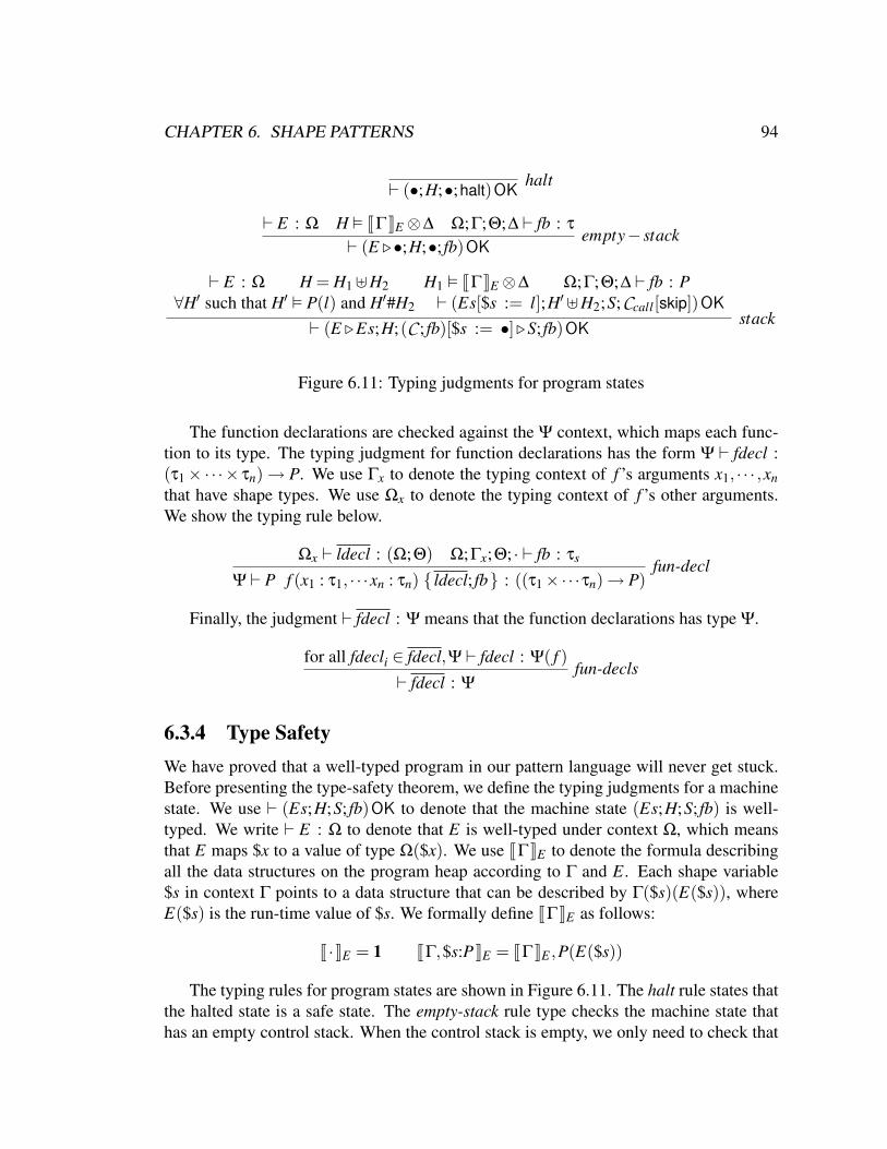
CHAPTER 6. SHAPE PATTERNS 94
` (•;H;•;halt)OKhalt
` E : Ω H JΓKE ⊗∆ Ω;Γ;Θ;∆ ` fb : τ
` (E .•;H;•; fb)OKempty− stack
` E : Ω H = H1]H2 H1 JΓKE ⊗∆ Ω;Γ;Θ;∆ ` fb : P∀H′ such that H′ P(l) and H′#H2 ` (Es[$s := l];H′]H2;S;Ccall[skip])OK
` (E .Es;H;(C ; fb)[$s := •].S; fb)OKstack
Figure 6.11: Typing judgments for program states
The function declarations are checked against the Ψ context, which maps each func-tion to its type. The typing judgment for function declarations has the form Ψ ` fdecl :(τ1×·· ·× τn)→ P. We use Γx to denote the typing context of f ’s arguments x1, · · · ,xnthat have shape types. We use Ωx to denote the typing context of f ’s other arguments.We show the typing rule below.
Ωx ` ldecl : (Ω;Θ) Ω;Γx;Θ; · ` fb : τs
Ψ ` P f (x1 : τ1, · · ·xn : τn) ldecl; fb : ((τ1×·· ·τn)→ P)fun-decl
Finally, the judgment ` fdecl : Ψ means that the function declarations has type Ψ.
for all fdecli ∈ fdecl,Ψ ` fdecl : Ψ( f )` fdecl : Ψ
fun-decls
6.3.4 Type SafetyWe have proved that a well-typed program in our pattern language will never get stuck.Before presenting the type-safety theorem, we define the typing judgments for a machinestate. We use ` (Es;H;S; fb)OK to denote that the machine state (Es;H;S; fb) is well-typed. We write ` E : Ω to denote that E is well-typed under context Ω, which meansthat E maps $x to a value of type Ω($x). We use JΓKE to denote the formula describingall the data structures on the program heap according to Γ and E. Each shape variable$s in context Γ points to a data structure that can be described by Γ($s)(E($s)), whereE($s) is the run-time value of $s. We formally define JΓKE as follows:
J ·KE = 1 JΓ,$s:PKE = JΓKE ,P(E($s))
The typing rules for program states are shown in Figure 6.11. The halt rule states thatthe halted state is a safe state. The empty-stack rule type checks the machine state thathas an empty control stack. When the control stack is empty, we only need to check that
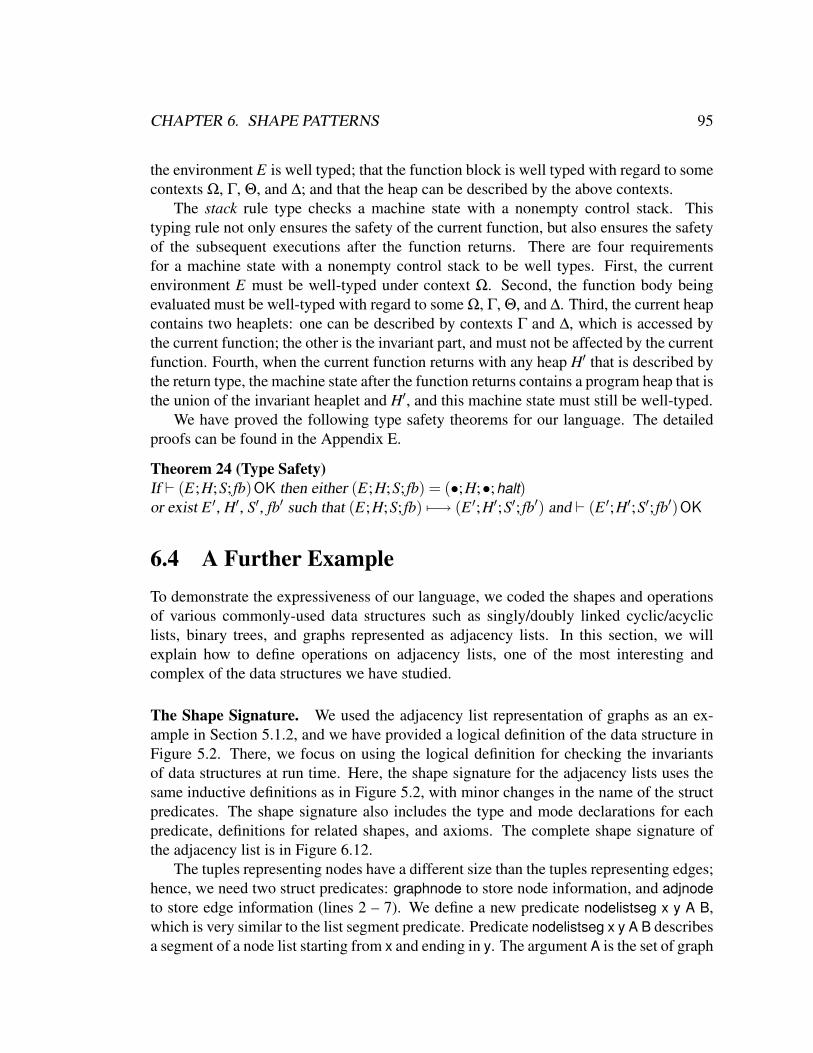
CHAPTER 6. SHAPE PATTERNS 95
the environment E is well typed; that the function block is well typed with regard to somecontexts Ω, Γ, Θ, and ∆; and that the heap can be described by the above contexts.
The stack rule type checks a machine state with a nonempty control stack. Thistyping rule not only ensures the safety of the current function, but also ensures the safetyof the subsequent executions after the function returns. There are four requirementsfor a machine state with a nonempty control stack to be well types. First, the currentenvironment E must be well-typed under context Ω. Second, the function body beingevaluated must be well-typed with regard to some Ω, Γ, Θ, and ∆. Third, the current heapcontains two heaplets: one can be described by contexts Γ and ∆, which is accessed bythe current function; the other is the invariant part, and must not be affected by the currentfunction. Fourth, when the current function returns with any heap H′ that is described bythe return type, the machine state after the function returns contains a program heap that isthe union of the invariant heaplet and H′, and this machine state must still be well-typed.
We have proved the following type safety theorems for our language. The detailedproofs can be found in the Appendix E.
Theorem 24 (Type Safety)If ` (E;H;S; fb)OK then either (E;H;S; fb) = (•;H;•;halt)or exist E ′, H′, S′, fb′ such that (E;H;S; fb) 7−→ (E ′;H′;S′; fb′) and ` (E ′;H′;S′; fb′)OK
6.4 A Further ExampleTo demonstrate the expressiveness of our language, we coded the shapes and operationsof various commonly-used data structures such as singly/doubly linked cyclic/acycliclists, binary trees, and graphs represented as adjacency lists. In this section, we willexplain how to define operations on adjacency lists, one of the most interesting andcomplex of the data structures we have studied.
The Shape Signature. We used the adjacency list representation of graphs as an ex-ample in Section 5.1.2, and we have provided a logical definition of the data structure inFigure 5.2. There, we focus on using the logical definition for checking the invariantsof data structures at run time. Here, the shape signature for the adjacency lists uses thesame inductive definitions as in Figure 5.2, with minor changes in the name of the structpredicates. The shape signature also includes the type and mode declarations for eachpredicate, definitions for related shapes, and axioms. The complete shape signature ofthe adjacency list is in Figure 6.12.
The tuples representing nodes have a different size than the tuples representing edges;hence, we need two struct predicates: graphnode to store node information, and adjnodeto store edge information (lines 2 – 7). We define a new predicate nodelistseg x y A B,which is very similar to the list segment predicate. Predicate nodelistseg x y A B describesa segment of a node list starting from x and ending in y. The argument A is the set of graph

CHAPTER 6. SHAPE PATTERNS 96
1 graph2 struct graphnode: (+, sf) ptr(graphnode)3 –> (–int, (–, sf) ptr(graphnode), (–,sf ) ptr(adjnode))4 –> o.5 struct adjnode: (+, sf) ptr(adjnode)6 –> ((–, sf) ptr(graphnode), (–,sf) ptr(adjnode))7 –> o.8 graph : (+, sf) ptr(graphnode) –> o.9 nodelist : (+, sf) ptr(graphnode)10 –> (–, sf) ptr(graphnode) set11 –> (–, sf) ptr(graphnode) set12 –> o.13 nodelistseg : (+, sf) ptr(graphnode)14 –> (+, unsf sf) ptr(graphnode)15 –> (–, sf) ptr(graphnode) set16 –> (–, sf) ptr(graphnode) set17 –> o.18 adjlist : (+, sf) ptr(adjnode) –> (–, sf) ptr(graphnode) set –> o.19 graph X o– nodelist X A B, O(B <= A).20 nodelist X A B o– O(X = 0), O(A = [ ]), O(B = [ ]);21 graphnode X ¡d, next, adjl> , adjlist adjl G, nodelist next A1 B1,22 O(A = [X] U A1), O(B = B1 U G).23 nodelistseg X Y A B o– O(X = Y), O(A = [ ]), O(B = [ ]);24 graphnode X (d, next, adjl), adjlist adjl G,25 nodelistseg next Y A1 B1, O(A = [X] U A1), O(B = B1 U G).26 adjlist X B o– O(X = 0), O(B = [ ]);27 adjnode X (n, next), adjlist next B1, O(B = [n] U B1).28 with29 nodelist X A B o– nodelistseg X Y A1 B1, nodelist Y A2 B2,30 O(A = A1 U A2), O(B = B1 U B2).31
Figure 6.12: Shape signature for graphs
nodes in this segment, and the argument B is the set of graph nodes that have at least oneincoming edge from the set of graph nodes in A. Lastly, we define an axiom to describethe relationship between a node list and a node list segment (line 29 – 30).
Graph Operations. We have coded and verified the most important operations ongraphs, including insertion and deletion of both nodes and edges. The most interesting
CHAPTER 6. SHAPE PATTERNS 97
1 graph delnode(graph $g, ptr(graphnode) $n)· · ·
20 $g := delEdgeNode($g, $n);21 switch $g of :[root x, O(ppre = $pre), O(pn = $n),22 nodelistseg x ppre A1 B1,23 graphnode ppre (dpre, pn, adjpre),24 adjlist adjpre G1,25 graphnode pn (dp, nextp, adjp),26 adjlist adjp G2,27 nodelist nextp A2 B2,28 O(A = A1 U [ppre] U A2),29 O(B = B1 U G1 U G2 U B2),30 O(B <= A)] –>
· · ·45 free pn;46 $g:graph := [root x, nodelistseg x ppre A1 B1,47 graphnode ppre (dpre, nextp, adjpre),48 adjlist adjpre G1,49 nodelist nextp A2 B2]
· · ·65 return $g;66
Figure 6.13: Code snippet of the node deletion function
operation is node deletion. Each node may be pointed to by arbitrarily many edges, soproperly deleting a node requires that all edges pointing to it are deleted. We present partof the delnode function in Figure 6.13.
The first argument, $g, is the adjacency list and the second argument, $n, is a pointerto the node in $g to be deleted. Before we can safety remove $n from $g, we have todelete all the pointers to $n from the adjacency lists of all the other nodes in the graph.On line 20, function delEdgeNode does precisely that.
Next, we use a switch statement (lines 21 – 49) to examine the shape of $g and delete$n from $g. In the code snippet, we only present one case of the switch statement. Nowwe explain how we check that the graph invariants are maintained. The shape pattern(lines 21 – 30) describes the shape of $g before deleting node $n, which is illustrated inFigure 6.14. In this case, we assume that stack variable $pre points to the predecessorof $n in the node list. On line 45, we free node $n. Then we reassemble $g using the

CHAPTER 6. SHAPE PATTERNS 98
ppre
pn
adjlist adjpre G1
adjlist adjp G2
nodelist nextp A2 B2
nodelistseg x ppre A1 B1
adjpnextpdp
adjprepndpre($pre)
($n)
Figure 6.14: Graph before deleting node $n
ppre adjlist adjpre G1
nodelist nextp A2 B2
nodelistseg x ppre A1 B1
adjprenextpdpre($pre)
Figure 6.15: Graph after deleting node $n
remainder of the graph (lines 46 – 49). We illustrate the shape of $g after deleting $n inFigure 6.15.
The shape assignment is valid because when no edges remain, the node $n to bedeleted appears in set A but not set B of a valid (nodelist X A B) predicate. We obtain thiscrucial fact from the shape pattern between lines 21 and 30, which contains the constrainB< = A. Notice that B is the set of graph nodes with at least one incoming edge, andA is the set of all graph nodes except node $n. This fact provides sufficient informationthat one can then delete the node and reform the graph, confident it contains no danglingpointers.
If programmers attempt to delete a node while edges remain pointing to it, in otherwords if they forget to call the delEdgeNode function or the delEdgeNode function isincorrectly written, a run-time error will occur when pattern matching the constraint B<= A on line 30. On the other hand, if the programmer did not write the constraint B<= A in the shape pattern of the switch statement, the shape assignment between lines 46and 49 will not type check, because it is impossible to convince the type system that theremaining data structure satisfies the definition of a graph. In particular, the set constrainton line 11 of Figure 6.12 (B <= A) will fail.
6.5 ImplementationWe implemented a prototype interpreter and type checker for our pattern language inSML/NJ. The interpreter contains a pattern-matching decision procedure module, whichis built on the rules in Figure 6.4. As part of the type checker, we implemented a simpletheorem prover that check the validity of the shape patterns. We also implemented amodule for mode analysis, which is invoked during type checking to verify the well-modedness of the logical definitions and the shape patterns. Finally, with the help of
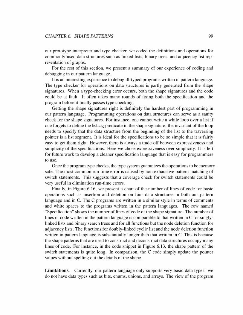
CHAPTER 6. SHAPE PATTERNS 99
our prototype interpreter and type checker, we coded the definitions and operations forcommonly-used data structures such as linked lists, binary trees, and adjacency list rep-resentation of graphs.
For the rest of this section, we present a summary of our experience of coding anddebugging in our pattern language.
It is an interesting experience to debug ill-typed programs written in pattern language.The type checker for operations on data structures is partly generated from the shapesignatures. When a type-checking error occurs, both the shape signatures and the codecould be at fault. It often takes many rounds of fixing both the specification and theprogram before it finally passes type checking.
Getting the shape signatures right is definitely the hardest part of programming inour pattern language. Programming operations on data structures can serve as a sanitycheck for the shape signatures. For instance, one cannot write a while loop over a list ifone forgets to define the listseg predicate in the shape signature; the invariant of the loopneeds to specify that the data structure from the beginning of the list to the traversingpointer is a list segment. It is ideal for the specifications to be so simple that it is fairlyeasy to get them right. However, there is always a trade-off between expressiveness andsimplicity of the specifications. Here we chose expressiveness over simplicity. It is leftfor future work to develop a cleaner specification language that is easy for programmersto use.
Once the program type checks, the type system guarantees the operations to be memory-safe. The most common run-time error is caused by non-exhaustive pattern-matching ofswitch statements. This suggests that a coverage check for switch statements could bevery useful in elimination run-time errors.
Finally, in Figure 6.16, we present a chart of the number of lines of code for basicoperations such as insertion and deletion on four data structures in both our patternlanguage and in C. The C programs are written in a similar style in terms of commentsand white spaces to the programs written in the pattern languages. The row named“Specification” shows the number of lines of code of the shape signature. The number oflines of code written in the pattern language is comparable to that written in C for singly-linked lists and binary search trees and for all functions but the node deletion function foradjacency lists. The functions for doubly-linked cyclic list and the node deletion functionwritten in pattern language is substantially longer than that written in C. This is becausethe shape patterns that are used to construct and deconstruct data structures occupy manylines of code. For instance, in the code snippet in Figure 6.13, the shape pattern of theswitch statements is quite long. In comparison, the C code simply update the pointervalues without spelling out the details of the shape.
Limitations. Currently, our pattern language only supports very basic data types: wedo not have data types such as bits, enums, unions, and arrays. The view of the program
CHAPTER 6. SHAPE PATTERNS 100
Data structures Operations/Specifications Pattern language CSingly linked acyclic list Specification 12 -
Insertion 16 16Deletion 15 15
Doubly linked cyclic list Specification 13 -Insertion 40 26Deletion 43 24
Binary search tree Specification 10 -Insertion 18 24Deletion 74 60
Adjacency list Specification 40 -representation Edge insertion 9 3of graphs Edge deletion 14 13
Node insertion 5 4Node deletion 90 66
Figure 6.16: Comparison of lines of code.
memory is quite simple as well: we assume every object takes up one word. We leaveextending our language to include other data types for future work.
The biggest limitation of our system is the high run-time cost of examining each datastructure when a shape pattern is matched against the heap. These checks are needed tomake sure that the heap have the desired shape. This means that for each while loop, thedata structures that are examined in the conditional expression will have to be traversedonce per loop execution. For future work, we plan to look into how to eliminate partof or all of the dynamic checks either by memorizing previous results at run time or byapplying even more powerful static analysis.
Chapter 7
Related Work
In this chapter, we survey related work. The overall goal of this thesis is to developlogics and tools to prove formal properties of programs that manipulate and deallocateheap-allocated data structures. There are three main technical components in this thesis:a new substructural logic, ILC, for describing program memory; a static and a dynamicverification system for imperative programs using ILC as specification language; and anew imperative language using ILC formulas as language constructs to ensure memorysafety. Many projects verify similar program properties as the systems presented in thisthesis. These projects took a variety of approaches, ranging from model checking to dataflow analysis to type systems. Some use formal logics to describe the program invariants,others do not. Almost all the verification systems check simple memory-safety conditions(no null-pointer differencing, no dangling pointer dereferencing, and no buffer overrun).Some systems (including ours) check more complex invariants of the heap-allocated datastructures, such as the shapes of the data structures. In this chapter, we compare our workwith projects that are most closely related to ours. We focus on systems that took similarapproaches to check the same program properties as ours. We organize our related workinto three main categories: logics describing program memory, verification systems forimperative programs, and new safe imperative languages.
7.1 Logics Describing Program HeapsThe first step of formally reasoning about the behavior of programs that manipulate heap-allocated data structures is to represent (model) the invariants of those data structuresin formal logics. In developing techniques for proving the correctness of imperativeprograms and analyzing the shape properties of data structures, researchers have comeup with logics of different flavors to describe the invariants of data structures allocatedon the heap. In this section, we discuss three such logics: monadic second-order logic,Kleene’s three-valued logic with transitive closure, and separation logic. These logics
101
CHAPTER 7. RELATED WORK 102
have already been put to use in verification systems to describe and reason about theshapes of data structures.
Graph Types developed by Klarlund et al. describe the shape of a data structureby its tree-shaped backbone and extra pointers to the nodes on the backbone [43]. Theinvariants of graph type structures can be expressed in a decidable fragment of monadicsecond-order logic. One limitation is that only data structures with tree-shaped backbonescan be described by graph types. We do not have such restriction on the shapes of thedata structures that can be described in our logic. However, for all practical purposes,most commonly used data structures such as lists and trees are expressible as graphtypes. Initially, graph types focus on describing the shape invariants of data structuresand ignore constraints on data. In their later work, the authors of graph types showedhow to express the ordering of keys on data structures such as binary search tree in adecidable fashion [53]. It is not obvious, if more general constraints were added, howthe decidability result would be affected. On the other hand, our logic separates thesubstructural reasoning from the constraint-based reasoning. We identified a fragment ofour logic that is decidable modulo the constraint-based reasoning. More precisely, thisdecidable fragment of ILC has a substructural reasoning component and a constraint-based reasoning component. We can plug in different constraint domains depending onthe invariants we would like to express. As long as the constraint domain of concern isdecidable, we obtain a decidable logic. There have been questions as to whether sub-structural logics can be encoded in monadic second-order logic so that MONA [42, 30]tool can be used for theorem proving. As Berdine et al. pointed out, it is not obvious howto give a compositional interpretation of the multiplicative conjunction of substructurallogic in second-order monadic logic [6].
Sagiv et al. have used Kleene’s three-valued logic with transitive closure [68] todescribe the shapes of linked data structures in their work on shape analysis [67]. Theabstractions of the stores are represented by “three-valued structures”. The structure ofthe heap is captured by a set of unary predicates that describe the point-to relationshipbetween stack variables and heap locations, and a set of binary predicates that describethe point-to relationship between heap locations. The logical structure also includes“summary” nodes, each of which represents multiple heap locations. In a three-valuedstructure, a predicate is evaluated to 1, if the predicate is true; 0, if the predicate is false;and 1
2 , if it is unknown. The additional value 12 allows one three-valued structure to
describe a set of concrete stores. The three-valued structures are further refined by usersupplied “instrumental predicates” which describes the reachability, acyclic properties,and sharing properties that are specific to the shapes of individual data structures. Incomparison, we do not need to express the reachability properties explicitly when describ-ing the shapes of data structures using substructural logics; instead, we use inductivelydefined predicates. When used in verification, the instrumental predicates have to beupdated globally when the data structures are modified. In comparison, in verification
CHAPTER 7. RELATED WORK 103
systems using substructural logic, the effect of the operation on one heap-cell is local,and does not have global effects on the entire formula describing the heap.
After all, the basic reasoning principles of monadic second-order logic and Kleene’sthree-valued predicate logic with transitive closure are fundamentally different from thatof the substructural logics where each assumption has to be used exactly once. The spatial(multiplicative) conjunction in substructural logics allows us to talk about the disjointnessof two heaplets concisely, and provide us with the ability to describe each individualpiece of the heap in isolation. Consequently, we are able to reason about the effect of anupdate to the data structures locally, which gives us an edge in reasoning about programsthat alter heap-allocated data structures. Interestingly, both graph types and three-valuedlogic representations of the store require some sort of separation of the program heap.Graph types require the store (exclude the extra pointers) to be disjoint acyclic backbonesspanning the heap. The heap locations are unique in three-valued logical abstraction ofthe store. It is evident that isolating the data structures (heap chunks) being operated onfrom the rest of the program heap is key to reasoning about complex heap-allocated datastructures in any case.
Most closely related to our logic is separation logic [35, 58, 66]. Separation logicextends a fragment of the logic of bunched implication (BI) [57] with recursively definedpredicates and axioms about lists and trees. The multiplicative fragment of ILC has thesame no-weakening and no-contraction properties as the multiplicative fragment of BI.BI and separation logic have an additive implication and an additive conjunction, whichdo not appear in our logic. Due to the special additive conjunction and implication,the logical contexts of BI are tree-shaped. To reduce the complexity of theorem proving,researchers have chosen to modify the proof theory of separation logic slightly by placingall the “pure formulas” in one zone and the formulas related to the heap in another. Thisarrangement is quite similar to what we have in ILC. We have developed and analyzedthis aspect of the logic from a formal proof-theoretic perspective. So far separationlogic has been focusing on verifying the shapes of data structures, therefore most of thepure formulas are limited to equality and inequality on integers. Reasoning about thesesimple arithmetic constraints has been hard coded into the proof system. More complexconstraints will have to be considered when the reasoning goes beyond the shapes ofdata structures, for instance, the ordering of keys which requires reasoning about partialorder on integers. In order to verify more general invariants of data structures, the logicthat is used to describe program properties should be flexible enough to incorporateany first-order theory that may be used to describe the program invariants. Our maingoal of developing ILC is precisely to address this issue. ILC allows general constraintdomains to be used in describing the program invariants. ILC’s proof theory modularlycombines substructural reasoning with general constraint-based reasoning in a principledway so that we can use existing linear logic theorem provers and off-the-shelf decisionprocedures to construct a theorem prover for our logic. Aside from the linear contextwhich corresponds to the context containing heap states in separation logic, ILC has

CHAPTER 7. RELATED WORK 104
an extra context that contains “heap-free” formulas, which can be used any number oftimes in the proof construction. For instance, axioms about lists and trees are “heap-free”formulas. Separation logic has hard coded those axioms into its proof system as well.One final note, separation logic with lists and tree axioms is complete with regard to thestore model, while ours is not. As we have discussed in Section 3.5, for the purposeof program verification, incompleteness should not prevent us from using ILC to verifyimperative programs.
7.2 Verification Systems for Imperative LanguagesOver the past twenty years, there have been several successful verification systems forpointer programs (e.g. [28, 37, 53, 17, 29, 79, 11, 7, 36]). Researchers have exploredusing different methods of checking properties of imperative programs. For instances,Blast [7] and F-Soft [36] are model checkers for C programs. Prefix [11] uses a path-sensitive data-flow analysis on C programs. Currently, these systems only check memorysafety, and do not check invariants of heap-allocated data structures such as the shapes ofthe data structures. Incidentally, systems that check the invariants of data structures uselogics we discussed in the previous section as the underlying specification languages fordescribing and reasoning about those invariants. Since our verification systems also usea logic (ILC) as the specification language and verify the invariants of data structures,those systems are most closely related to our work. In this section, we survey theseverification systems, discuss different verification techniques used in these systems andcompare them with our verification systems.
PALE [53] can automatically verify programs that manipulate data structures express-ible as graph types. Similar to our static verification system, PALE requires programs tobe annotated with pre- and post-conditions and loop invariants. The specifications andthe program are translated into monadic second-order logical formulas. These formulasare then processed by the MONA tool to check validity and to extract counterexamplesif the verification fails. Our verification system does not have the ability to extractcounterexamples. PALE uses forward reasoning technique which means that at eachfunction call site, the formula describing the current store need to be separated into twoparts: the precondition for the callee, and an invariant part describing the part of the storethat will not be modified by the callee. In order for the system to be sound, these twoparts should describe two disjoint pieces of the program heap. PALE does not check thedisjointness property automatically. However, the authors gave heuristics for checking thesufficient conditions for this disjointness property. We use a backward reasoning scheme,where the disjointness of the invariant part and the callee’s precondition is embodied inthe verification condition of the function call command.
TVLA [45] uses the shape analysis based on three-valued logic to verify that theinvariants of the data structures are preserved by the programs. It takes as input, a

CHAPTER 7. RELATED WORK 105
description of the store before the execution of the program and the description of thedata structures. The precondition describing the store is symbolically executed againstthe programs and produces the abstractions of the store at each program point. Oneadvantage of TVLA is that it does not need annotations for loop invariant. TVLA usesshape analysis algorithm to synthesize a least fixed point for the loop invariants. However,users have to provide “instrumental predicates” for each data structures and the updateoperational semantics for these “instrumental predicates”. The precision of the analysismay be compromised as a result of imprecise instrumental predicates. Being able to inferloop invariants is a great advantage over our verification system where loop invariantshave to be provided. Ideally, we would like to combine the work on shape analysiswith our verification system, and use the shape analysis techniques such at the onespresented in Sagiv [67] and Guo’s recent work [27], to infer loop invariants for us. Itwould definitely be one more step forward towards automated verification.
More recently, Berdine etc. have developed Smallfoot [6], a static verification toolfor imperative programs using separation logic. Programs are annotated with pre-, post-conditions and loop invariants, which are separation logic formulas. What sets Smallfootand our static verification system apart from other verification systems such as PALE andTVLA is that the underlying substructural logics allow local reasoning about the heap,and we do not need to keep track of any global parameters to deal with aliasing. Theverification rules in our system are almost identical to those backward reasoning rulesusing Separation Logic [35, 58, 66]. Smallfoot uses a forward reasoning technique, andsymbolically executes logical formulas [41]. This means that similar to PALE, Smallfoothas to split a formula into two disjoint parts at a function call, which they call “inferenceof the frame rule”. While our system has no need to do so, because our system usesbackward reasoning. Symbolically executing the program on logical formulas allowsSmallfoot to operate on a quantifier-free fragment of separation logic. Our verificationrules need both universal and existential quantification. From theorem proving point ofview, the theorem proving is much simpler for a quantifier-free fragment. The proofrules in Smallfoot have hard-coded all the axioms for lists and trees. We hard-codedthe unrolling of the recursive data structures into the verification generation rules. Otheraxioms such as rolling the data structures back are axioms in the unrestricted context inthe proof system. It is important for researchers developing both systems to discovernecessary axioms about the shapes of data structures. So far, development of necessaryaxioms has been a limiting factor for programmers attempting to use these verificationsystem effectively. Finally, in addition to verify sequential programs, Smallfoot alsoverify the data-race free condition for concurrent programs.
One important new aspect of our work is that in addition to developing a staticverification system, we also created a dynamic verification system that uses the sameunderlying logic. We can easily join the static and dynamic verification systems intoone. In this combined system, users have the flexibility to choose between static anddynamic verification of programs. This flexibility allows them to achieve the desired

CHAPTER 7. RELATED WORK 106
balance between the overall cost of verification, the desired safety guarantees and therun-time overhead. PALE, TVLA and Smallfoot are all strictly static verification tools.
7.3 Safe Imperative LanguagesAside from verification systems for existing imperative languages, many projects aimat developing novel type systems and new language features to ensure the memory-safety of imperative programs. In this section, we examine some of the safe imperativelanguages, and compare their features with our pattern language, which uses high-levellogical formulas to perform safe operations on data structures.
CCured [55], a C program transformation and analysis system, gives a strong typesystem for C to ensure memory-safety. CCured categorized pointers into two kinds:safe pointers that are strongly typed; and wild pointers that are untyped. Operations onsafe pointers can be proven memory-safe statically by the type system, whereas run-timechecks have to be added before operations on wild pointers. CCured prevents errors dueto dereferencing dangling pointers by making the free instruction do nothing and using aBoehm-Demers-Weiser garbage collector [9]. Cyclone [40, 26] is a type-safe dialect ofC. Cyclone provides a variety of safe memory management including statically scopedregions, dynamic regions, and unique pointers. Programmers can deallocate dynamicregions and free objects pointed to by unique pointers explicitly. For ordinary heappointers Cyclone took a similar approach as CCured. Cyclone makes free a no-op andrelies on a garbage collector to reclaim memory. The type system of our pattern languageand other safe imperative languages that support explicit deallocation [14, 19, 69, 77, 13,54, 80] including Cyclone share the same principle of using linear capabilities to trackaccessible portion of the heap. CCured and Cyclone are general-purpose languages, whileour pattern language is a special purpose language for developing libraries for complexrecursive data structures. Our type system not only ensures memory-safety, but alsoensures that data structures conform to the specification of their shapes.
Walker’s alias types for recursive data structures [77] can encode the shapes of listsand trees in a pseudo-linear type system. The fundamental idea for expressing the shapeinvariants of recursive data structures is quite similar to ours. Since their type systemtargets intermediate language for certifying compilation, they can rely on compilers togenerate the coercion instructions to explicitly roll and unroll recursive types. Their typesystem does not need to use a theorem prover, and also much less expressive than ours.Our language use logical formulas to construct and deconstruct recursive data structures,so our type system use a theorem prover to prove the soundness of the constructionand deconstruction of data structures. Being able to use logical formulas to define datastructures also allows us to express data constraints of the data structures, for instancesthe constraints of key ordering in binary search trees, and the constraint of heights onbalanced trees, which alias types can not express.

CHAPTER 7. RELATED WORK 107
Several researchers have used declarative specifications of complex data structures togenerate code and implement pattern-matching operations. For example, Fradet and LeMetayer developed shape types [22] by using context-free graph grammars to define re-cursive data structures. They then developed an imperative language, called Shape-C. InShape-C, operations on data structures are edge rewriting rules on the graph grammar. Analgorithm is given to prove each rewriting transformation maintains the shape invariantsdefined by the graph grammar. They also gave an algorithm to translate programs writtenin Shape-C to equivalent C programs. One limitation of shape types is that the operationson data structures require the invariants of the data structures to hold at all times. Inpractice, the invariants of data structures are often temporarily violated, and restored laterin the program. Our type system allow a data structure to be deconstructed as long as theshape invariants are restored when the data structure is re-assembled. Another limitationof shape types is that it did not come with a facility for expressing relations betweendifferent shapes similar to our axioms, and consequently it appears that they cannot beused effectively inside while loops or other looping constructs.
What is unique to our language is that logic formulas are used directly as languageconstructs to manipulate data structures. We aim to replace low-level pointer manipula-tion with higher-level data structure specification and adopt the “correct by construction”approach. Most importantly, our language has the promise of synergy with new verifica-tion techniques based on substructural logics and with modern type systems for resourcecontrol, including those in Vault [14] and Cyclone [25, 31].

Chapter 8
Conclusion and Future Work
In this thesis, we have defined a new substructural logic, ILC, that modularly combinessubstructural reasoning with general constraint-based reasoning to reason about the mem-ory safety and shape invariants of pointer programs. In this section, we summarize thecontributions of this thesis and propose future research directions.
8.1 ContributionsThis thesis makes the following contributions.
• We developed ILC as a foundation for reasoning about the program heap. Theproof theory of ILC modularly combines linear logic reasoning with constraint-based reasoning, and therefore enables us to develop automated theorem proversfor ILC by using existing linear logic theorem provers and off-the-shelf decisionprocedures.
• We developed a sound decision procedure for an expressive fragments of ILC,which we later use in various verification systems. The decidable nature of thelogical reasoning is crucial to the development of termination verification systemsusing ILC.
• We developed a static verification system for pointer programs that is decidable ifthe logical annotations of the programs’ pre- and post-conditions and loop invari-ants fall into the decidable fragment of ILC.
• We proposed to use ILC as a language of contracts for specifying heap-shapeproperties. Unlike the ad hoc, unstructured heap-shape contracts one might write innative code, these contracts serve as clear, compact and semantically well-defineddocumentation of heap-shape properties.
108

CHAPTER 8. CONCLUSION AND FUTURE WORK 109
• We showed how to combine our static and the dynamic verification techniques,both of which use ILC as the specification language. In such a combined system,the users have great flexibility in choosing different combinations of techniques toobtain the balance between the strength of safety guarantees, the cost of verifica-tion, and run-time overhead.
• We proposed a new programming language in which logical specifications, ratherthan low-level pointer operations, drive safe construction and manipulation of so-phisticated heap-allocated data structures. We incorporate the verification tech-niques into the type systems of this language and ensure that well-typed programsare memory safe, and that the shape invariants of the data structures are preservedduring the execution of the program.
8.2 Future workWhile trying to develop tools and techniques for verifying pointer programs, researchershave advanced the state of the art in logic and type systems. The verification of pointerprograms continues to pose challenges to programming language researchers. In thissection, we survey some of the directions for future research.
Automatic Generation of Axioms for Recursive Data Structures. In reasoning aboutrecursively defined data structures, researchers need to identify the set of useful axiomsabout these data structures. For instance, to reason about a program that operates on lists,in addition to the list definition, we need an axiom to state that two joint list segments canbe rolled into one list segment. Currently, no one has studied how to define a completeset of axioms for any given recursive data structure in a principled manner. It requires alot of special knowledge to write down all the axioms for any given data structure. If wecould automatically generate axioms for data structures, the verification system would bemore available to the average programmers who have less special knowledge about logic.
Separation and Inequality. One of the key reasons why substructural logic can de-scribe the program heap so elegantly is that by using the separating conjunction, we donot need to specify the inequality of distinct heap locations. However, in verifying pointerprograms, we need to define axioms to derive the inequality between heap locations fromthe disjointness of two parts of the heap. These axioms look less than elegant and theydepend on the specific definitions of data structures. It would be interesting to investigatehow to bridge this mismatch of specifying inequality between the substructural logic andthe programming languages in which the programs are written.
CHAPTER 8. CONCLUSION AND FUTURE WORK 110
Scalability. Substructural logics have shown to be able to describe and reason aboutprogram memory elegantly. However, recent research in using substructural logics to de-velop verification techniques and tools for pointer programs has had only limited success:the languages in which the programs can be verified are overly simple. These verificationsystems have not been put to test in face of a real sized program. The symbolic executionmethods using substructural logic, such as the one used in Smallfoot, face state explosionproblems as the size of the program grows. The backward verification generation methodswill generate a huge formula when the program size increases. In order for the verificationtechniques that use substructural logics to have a real impact on improving the reliabilityof software, one important future direction is to develop a verification system for realimperative languages like C. We need to address issues such as how to capture thememory-safety invariants of programs that contain pointer arithmetic and type castingof pointers, and how to make the system scalable.

Appendix A
Proofs in Logic Section
A.1 Proofs of Cut-Elimination of ILCLemma 25If for all i ∈ [1,3], Aeqi ∈Θ, Θ # t = s and Θ # Pa(t) then Θ # Pa(s).
Proof
By assumption,D1 :: Θ # t = s (1)D2 :: Θ # Pa(t) (2)
D1Θ,¬(t = s) # t = s,Pa(s)
Weakening
Θ,¬(t = s) # Pa(s) ¬T (3)D2
Θ,¬Pa(t) # Pa(t),Pa(s)Weakening
Θ,¬Pa(t) # Pa(s) ¬T (4)Θ,Pa(s) # Pa(s) (5)
By ∨T, (3), (4), (5),Θ,¬(t = s)∨¬Pa(t)∨Pa(s) # Pa(s) (6)
By ∀T,Θ,Aeq3 # Pa(s) (7)
By contraction,Θ # Pa(s) (8)
Lemma 26 (Reflexivity)If for all i ∈ [1,3], Aeqi ∈Θ, then Θ # t = t.
111
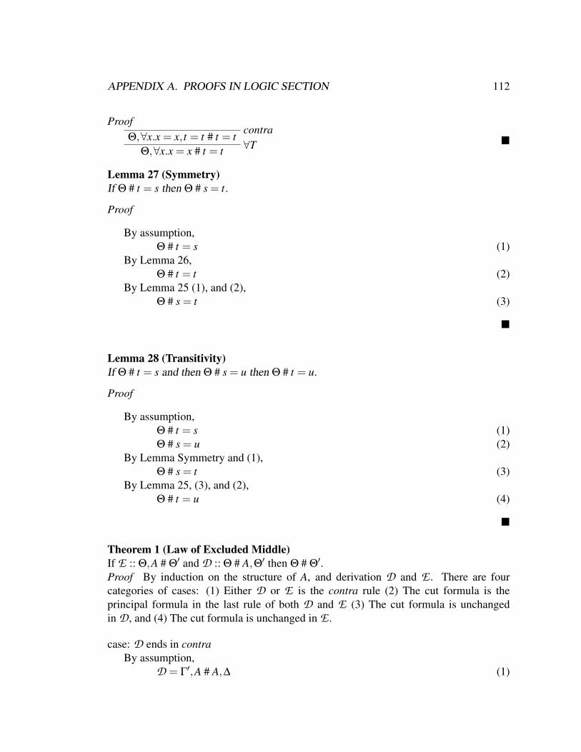
APPENDIX A. PROOFS IN LOGIC SECTION 112
Proofcontra
Θ,∀x.x = x, t = t # t = t∀T
Θ,∀x.x = x # t = t
Lemma 27 (Symmetry)If Θ # t = s then Θ # s = t.
Proof
By assumption,Θ # t = s (1)
By Lemma 26,Θ # t = t (2)
By Lemma 25 (1), and (2),Θ # s = t (3)
Lemma 28 (Transitivity)If Θ # t = s and then Θ # s = u then Θ # t = u.
Proof
By assumption,Θ # t = s (1)Θ # s = u (2)
By Lemma Symmetry and (1),Θ # s = t (3)
By Lemma 25, (3), and (2),Θ # t = u (4)
Theorem 1 (Law of Excluded Middle)If E :: Θ,A # Θ′ and D :: Θ # A,Θ′ then Θ # Θ′.Proof By induction on the structure of A, and derivation D and E . There are fourcategories of cases: (1) Either D or E is the contra rule (2) The cut formula is theprincipal formula in the last rule of both D and E (3) The cut formula is unchangedin D , and (4) The cut formula is unchanged in E .
case: D ends in contraBy assumption,
D = Γ′,A # A,∆ (1)
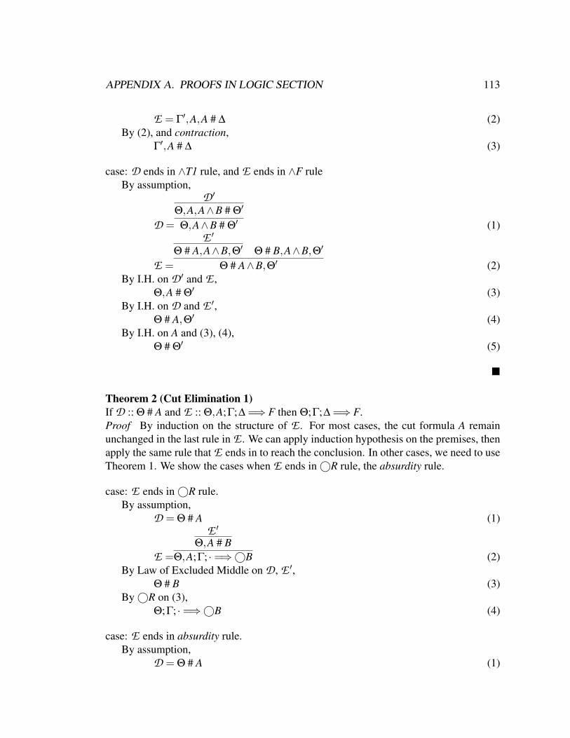
APPENDIX A. PROOFS IN LOGIC SECTION 113
E = Γ′,A,A # ∆ (2)By (2), and contraction,
Γ′,A # ∆ (3)
case: D ends in ∧T1 rule, and E ends in ∧F ruleBy assumption,
D =
D ′
Θ,A,A∧B # Θ′
Θ,A∧B # Θ′ (1)
E =
E ′
Θ # A,A∧B,Θ′ Θ # B,A∧B,Θ′
Θ # A∧B,Θ′ (2)By I.H. on D ′ and E ,
Θ,A # Θ′ (3)By I.H. on D and E ′,
Θ # A,Θ′ (4)By I.H. on A and (3), (4),
Θ # Θ′ (5)
Theorem 2 (Cut Elimination 1)If D :: Θ # A and E :: Θ,A;Γ;∆ =⇒ F then Θ;Γ;∆ =⇒ F.Proof By induction on the structure of E . For most cases, the cut formula A remainunchanged in the last rule in E . We can apply induction hypothesis on the premises, thenapply the same rule that E ends in to reach the conclusion. In other cases, we need to useTheorem 1. We show the cases when E ends in ©R rule, the absurdity rule.
case: E ends in ©R rule.By assumption,
D = Θ # A (1)
E =
E ′
Θ,A # BΘ,A;Γ; ·=⇒©B (2)
By Law of Excluded Middle on D , E ′,Θ # B (3)
By ©R on (3),Θ;Γ; ·=⇒©B (4)
case: E ends in absurdity rule.By assumption,
D = Θ # A (1)
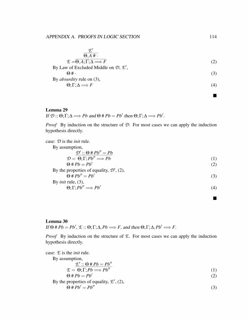
APPENDIX A. PROOFS IN LOGIC SECTION 114
E =
E ′
Θ,A # ·Θ,A;Γ;∆ =⇒ F (2)
By Law of Excluded Middle on D , E ′,Θ # · (3)
By absurdity rule on (3),Θ;Γ;∆ =⇒ F (4)
Lemma 29If D :: Θ;Γ;∆ =⇒ Pb and Θ # Pb = Pb′ then Θ;Γ;∆ =⇒ Pb′.
Proof By induction on the structure of D . For most cases we can apply the inductionhypothesis directly.
case: D is the init rule.By assumption,
D =D ′ :: Θ # Pb′′ = PbΘ;Γ;Pb′′ =⇒ Pb (1)
Θ # Pb = Pb′ (2)By the properties of equality, D ′, (2),
Θ # Pb′′ = Pb′ (3)By init rule, (3),
Θ;Γ;Pb′′ =⇒ Pb′ (4)
Lemma 30If Θ # Pb = Pb′, E :: Θ;Γ;∆,Pb =⇒ F, and then Θ;Γ;∆,Pb′ =⇒ F.
Proof By induction on the structure of E . For most cases we can apply the inductionhypothesis directly.
case: E is the init rule.By assumption,
E =E ′ :: Θ # Pb = Pb′′
Θ;Γ;Pb =⇒ Pb′′ (1)Θ # Pb = Pb′ (2)
By the properties of equality, E ′, (2),Θ # Pb′ = Pb′′ (3)

APPENDIX A. PROOFS IN LOGIC SECTION 115
By init rule on (3),Θ;Γ;Pb′ =⇒ Pb′′ (4)
Theorem 3 (Cut Elimination 2)
1. If D :: Θ;Γ;∆ =⇒ F and E :: Θ;Γ;∆′,F =⇒ F′ then Θ;Γ;∆,∆′ =⇒ F′.
2. If D :: Θ;Γ; ·=⇒ F and E :: Θ;Γ,F;∆ =⇒ F′ then Θ;Γ;∆ =⇒ F′.
Proof1. By induction on the structure of A, and derivation D and E . There are four categoriesof cases: (1) Either D or E is the init rule (2) The cut formula is the principal formulain the last rule of both D and E (3) The cut formula is unchanged in D , and (4) The cutformula is unchanged in E . We only apply 2 when the cut formula is strictly smaller.
case: D ends in init rule.By assumption,
D =D ′ :: Θ # Pb′ = PbΘ;Γ;Pb′ =⇒ Pb (1)
E = Θ;Γ;∆,Pb =⇒ F (2)By Lemma 30, D ′, (2),
Θ;Γ;∆,Pb′ =⇒ F (3)
case: E ends in init rule.By assumption,
E =E ′ :: Θ # Pb′ = PbΘ;Γ;Pb′ =⇒ Pb (1)
D = Θ;Γ;∆ =⇒ Pb′ (2)By Lemma 29, E ′, (2),
Θ;Γ;∆ =⇒ Pb (3)
case: ©A is the principal cut formulaBy assumption,
D =
D ′
Θ # AΘ;Γ; ·=⇒©A (1)
E =
E ′
Θ,A;Γ;∆ =⇒ FΘ;Γ;∆,©A =⇒ F (2)
By Theorem 2 on D ′ and E ′,Θ;Γ;∆ =⇒ F (3)

APPENDIX A. PROOFS IN LOGIC SECTION 116
2. By induction on the structure of E . For most cases, the principal cut formula isunchanged in the last rule in E . We can apply induction hypothesis on the premises, thenapply the same rule that E ends in to reach the conclusion. We show the case when Eends in copy rule.
case: E ends in copy rule.By assumption,
D = Θ;Γ; ·=⇒ F (1)
E =
E ′
Θ;Γ,F;∆,F =⇒ F′
Θ;Γ,F;∆ =⇒ F′ (2)By I.H. on D and E ′,
Θ;Γ;∆,F =⇒ F′ (3)By Theorem 3.1 on (3), (1),
Θ;Γ;∆ =⇒ F′ (4)
A.2 Proof for the soundness of logical deductionTheorem 6 If Θ;Γ;∆ =⇒ F and σ is a ground substitution for all the free variables inthe judgment, and M is a model such that M σ(Θ), and M;H σ(
N!Γ⊗
N∆) then
M;H σ(F).Proof By induction on the structure of the deviation D :: Θ;Γ;∆ =⇒ F
case: D =
D ′
Θ;Γ;∆,F1 =⇒ F2Θ;Γ;∆ =⇒ F1 ( F2
By assumption,σ is a grounding substitution (1)M σ(Θ) (2)M;H σ(
N(!Γ)⊗ (
N∆)) (3)
given heap H1 such that M;H1 σ(F1) (4)By semantics of ⊗,
M;H]H1 σ(N
(!Γ)⊗ (N
∆)⊗F1) (5)By I.H. on D ′ and (1), (2), (5),
M;H]H1 σ(F2) (6)By semantics of (, (4), (6),
M;H σ(F1 ( F2) (7)

APPENDIX A. PROOFS IN LOGIC SECTION 117
case: D =
D ′
Θ;Γ;∆ =⇒ F[t/x]Θ;Γ;∆ =⇒∃x.F
By assumption,σ is a grounding substitution (1)M σ(Θ) (2)M;H σ(
N(!Γ)⊗ (
N∆)) (3)
By I.H. on D ′ and (2), (3),M;H σ(F[t/x]) (4)M;H σ(F)[σ(t)/x] (5)
By semantics of ∃,M;H ∃x.(σ(F)) (6)M;H σ(∃x.(F)) (7)
case: D =
D ′
Θ;Γ;∆,F[a/x] =⇒ F′
Θ;Γ;∆,∃x:ST .F =⇒ F′
By assumption,σ is a grounding substitution (1)M σ(Θ) (2)M;H σ(
N(!Γ)⊗ (
N∆)⊗∃x:ST .F) (3)
By semantics of ⊗,H = H1]H2 st M;H1 σ(
N(!Γ)⊗ (
N∆)),
and M;H2 σ(∃x:ST .F) (4)By semantics of ∃,
there exists some integer t (if ST = Si), or some finite set t (if ST = Ss)such that M;H2 (σ, t/x)(F) (5)M;H2 (σ, t/a)(F[a/x]) (6)
By (4) and (6), and a is fresh in the judgment,M;H1]H2 (σ, t/a)(
N(!Γ)⊗ (
N∆)⊗F[a/x]) (7)
By I.H on D ′, (1),(7),M;H1]H2 (σ, t/a)(F′) (8)
By (4),(8), and a does not appear in F′,M;H σ(F′) (9)
case: D =
D ′
Θ # AΘ;Γ; ·=⇒©A
By assumption,σ is a grounding substitution (1)M σ(Θ) (2)M;H σ(
N(!Γ)) (3)

APPENDIX A. PROOFS IN LOGIC SECTION 118
By the semantics of ! and (3),H = /0 (4)
By the soundness of first order logic and D ′, (2),M σ(A) (5)
By the semantics of ©, (4), (5),M;H σ(©A) (6)
case: D =
D ′
Θ # ·Θ;Γ;∆ =⇒ F
By assumption,σ is a grounding substitution (1)M σ(Θ) (2)
By the soundness of first order logic and D ′, (2),M false (3)M does not exists therefore any conclusion from M exists follows. (4)
Lemma 31If M;H B then ∃n≥ 0, such that M;H n B.
Proof (sketch): By induction on the structure of B. Theorem 7 For all I ∈ ϒ, M; /0 ϒ I.Proof
By assumption,I = ∀x1. · · ·∀xn.(B1⊕·· ·⊕Bm) ( P (1)given any grounding substitution σ,dom(σ) = x1 · · ·xn (2)given any heap H, such that M;H σ(B1⊕·· ·⊕Bm) (3)
By the semantics of ⊕,there exists an integer i such that M;H σ(Bi) (4)
By Lemma 31,∃n≥ 0 such that M;H n Bi
By the semantics of user defined predicates,M;H n+1 σ(P) (5)M;H σ(P) (6)
By the semantics of ∀, and (,M; /0 ∀x1. · · ·∀xn.(B1⊕·· ·⊕Bm) ( P (7)
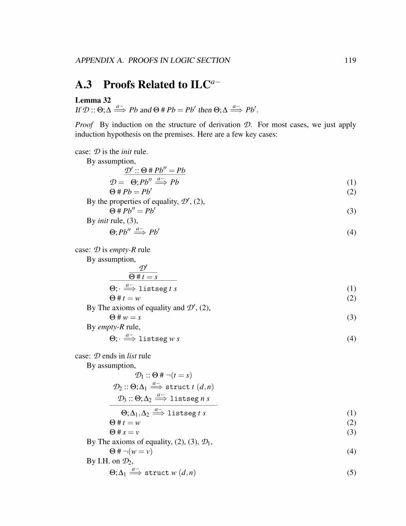
APPENDIX A. PROOFS IN LOGIC SECTION 119
A.3 Proofs Related to ILCa−
Lemma 32If D :: Θ;∆
a−=⇒ Pb and Θ # Pb = Pb′ then Θ;∆a−=⇒ Pb′.
Proof By induction on the structure of derivation D . For most cases, we just applyinduction hypothesis on the premises. Here are a few key cases:
case: D is the init rule.By assumption,
D =D ′ :: Θ # Pb′′ = Pb
Θ;Pb′′ a−=⇒ Pb (1)Θ # Pb = Pb′ (2)
By the properties of equality, D ′, (2),Θ # Pb′′ = Pb′ (3)
By init rule, (3),Θ;Pb′′ a−=⇒ Pb′ (4)
case: D is empty-R ruleBy assumption,
D ′
Θ # t = sΘ; · a−=⇒ listseg t s (1)Θ # t = w (2)
By The axioms of equality and D ′, (2),Θ # w = s (3)
By empty-R rule,Θ; · a−=⇒ listseg w s (4)
case: D ends in list ruleBy assumption,
D1 :: Θ # ¬(t = s)D2 :: Θ;∆1
a−=⇒ struct t (d,n)D3 :: Θ;∆2
a−=⇒ listseg n s
Θ;∆1,∆2a−=⇒ listseg t s (1)
Θ # t = w (2)Θ # s = v (3)
By The axioms of equality, (2), (3), D1,Θ # ¬(w = v) (4)
By I.H. on D2,Θ;∆1
a−=⇒ struct w (d,n) (5)

APPENDIX A. PROOFS IN LOGIC SECTION 120
By I.H. on D3,Θ;∆2
a−=⇒ listseg n v (6)By the list rule on (4), (5), (6), D1,
Θ;∆1,∆2a−=⇒ listseg w v (7)
Lemma 33If Θ # Pb = Pb′, E :: Θ;∆,Pb a−=⇒ D, and then Θ;∆,Pb′ a−=⇒ D.
Proof By induction on the structure of E . For most cases, Pb remain unchanged in E .We can apply induction hypothesis on the premises, then apply the same rule that E endsin to reach the conclusion.
Theorem 9 (Cut Elimination 2)If Θ;∆
a−=⇒ D and Θ;∆′,D a−=⇒ D′ then Θ;∆,∆′a−=⇒ D′.
ProofIt is very similar to the proof of Cut Elimination Theorem of ILC. Here we list the
cases when D or E ends in the two new rules concerning lists.
case: D ends in init rule.By assumption,
D =D ′ :: Θ # Pb′ = Pb
Θ;Pb′ a−=⇒ Pb (1)E = Θ;∆,Pb a−=⇒ D (2)
By Lemma 33, D ′, (2),Θ;∆,Pb′ a−=⇒ D (3)
case: E ends in init rule.By assumption,
E =E ′ :: Θ # Pb′ = Pb
Θ;Pb′ a−=⇒ Pb (1)D = Θ;∆
a−=⇒ Pb′ (2)By Lemma 32, E ′, (2),
Θ;∆a−=⇒ Pb (3)
case:E ends in list rule. We show the case when the cut formula is in the second premise,the other case when the cut formula is in the third premise is similar.
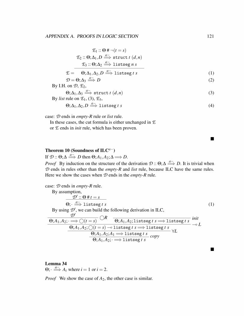
APPENDIX A. PROOFS IN LOGIC SECTION 121
E =
E1 :: Θ # ¬(t = s)E2 :: Θ;∆1,D
a−=⇒ struct t (d,n)E3 :: Θ;∆2
a−=⇒ listseg n s
Θ;∆1,∆2,Da−=⇒ listseg t s (1)
D = Θ;∆3a−=⇒ D (2)
By I.H. on D , E2,Θ;∆1,∆3
a−=⇒ struct t (d,n) (3)By list rule on E1, (3), E3,
Θ;∆1,∆2,Da−=⇒ listseg t s (4)
case: D ends in empty-R rule or list rule.In these cases, the cut formula is either unchanged in Eor E ends in init rule, which has been proven.
Theorem 10 (Soundness of ILCa−)If D :: Θ;∆
a−=⇒ D then Θ;A1,A2;∆ =⇒ D.Proof By induction on the structure of the derivation D :: Θ;∆
a−=⇒ D. It is trivial whenD ends in rules other than the empty-R and list rule, because ILC have the same rules.Here we show the cases when D ends in the empty-R rule.
case: D ends in empty-R rule.By assumption,
D ′ :: Θ # t = sΘ; · a−=⇒ listseg t s (1)
By using D ′, we can build the following derivation in ILC,D ′
©RΘ;A1,A2; ·=⇒©(t = s) init
Θ;A1,A2;listseg t s =⇒ listseg t s( L
Θ;A1,A2;©(t = s) ( listseg t s =⇒ listseg t s∀L
Θ;A1,A2;A1 =⇒ listseg t s copyΘ;A1,A2; ·=⇒ listseg t s
Lemma 34Θ; · a−=⇒ Ai where i = 1 or i = 2.
Proof We show the case of A2, the other case is similar.

APPENDIX A. PROOFS IN LOGIC SECTION 122
D1 D2 D3 empty-RΘ,¬(a = b);struct a (d,c),listseg c b a−=⇒ listseg a b
©LΘ;©(¬(a = b)),struct a (d,c),listseg c b a−=⇒ listseg a b
⊗LΘ;©(¬(a = b))⊗struct a (d,c)⊗listseg c b a−=⇒ listseg a b
( RΘ; · a−=⇒ ©(¬(a = b))⊗struct a (d,c)⊗listseg c b ( listseg a b
∀RΘ; · a−=⇒ ∀x.∀y.∀d.∀z.© (¬(x = y))⊗struct x (d,z)⊗listseg z y ( listseg x y
where
D1 =Θ,¬(a = b) # Θ,¬(a = b)contra
D2 = Θ;struct a (d,c) a−=⇒ struct a (d,c)init
D3 = Θ;listseg c b a−=⇒ listseg c binit
Theorem 11 (Completeness of ILCa−) If E :: Θ;A1,A2;∆ =⇒D and all the formulas in∆ are D, then Θ;∆
a−=⇒ D.Proof By induction on the structure of E :: Θ;A1,A2;∆ =⇒ D and the structure of D.Most cases invoke the induction hypothesis directly. In the case of copy rule, we useLemma 34.
case: E ends in the copy rule.By assumption,
E ′ :: Θ;A1,A2;∆,Ai =⇒ D′
Θ;A1,A2;∆ =⇒ D′ where i = 1 or 2 (1)By I.H. on E ′,
Θ;∆,Aia−=⇒ D′ (2)
By Lemma 34,Θ; · a−=⇒ Ai (3)
By Cut Elimination on (2), and (3),Θ;∆
a−=⇒ D′ (4)
A.4 Proof of the Soundness of Residuation CalculusIn this section, we present the proofs for the soundness of the residuation calculus.

APPENDIX A. PROOFS IN LOGIC SECTION 123
Θ,A #s A Contra
Θ #s A Θ #s BΘ #s A∧B ∧F
Θ,A #s A′
Θ,A∧B #s A′∧T1
Θ,B #s A′
Θ,A∧B #s A′∧T2
Θ #s truetrueF
Θ #s AΘ #s A∨B ∨F1 Θ #s B
Θ #s A∨B ∨F2Θ,A #s A′ Θ,B #s A′
Θ,A∨B #s A′∨T
Θ,false #s A falseT
Θ,A #s ·Θ #s ¬A ¬F Θ #s A
Θ,¬A #s B ¬T
Θ #s A[t/x] t ∈ STΘ #s ∃x:ST .A ∃F
Θ,A[a/x] #s B a is freshΘ,∃x:ST .A #s B ∃T
Θ #s A[a/x] a is freshΘ #s ∀x:ST .A ∀F
Θ,A[t/x] #s B t ∈ STΘ,∀x:ST .A #s B ∀T
Θ,A∨¬A #s BΘ #s B excluded-middle
Figure A.1: Sequent rules for classical first-order logic
A.4.1 An Alternative Sequent Calculus for Constraint ReasoningNotice that when the constraint-based reasoning interacts with the linear reasoning inILCa−, such as the ©R rule, we always use a derivation of a single conclusion. How-ever, the sequent calculus for constraint-based reasoning has multiple conclusions. Thispresents some challenge in finding a suitable inductive hypothesis in our proofs. There-fore, in this section, we define an alternative sequent calculus for constraint-based rea-soning in Figure A.1. To be able to still derive the law of excluded middle, we include anexcluded-middle rule.
We prove the formal properties of the single conclusion calculus. Most importantly,we prove that this new calculus is sound and complete with regard to the original calculus.
Lemma 35If Θ #s A and Θ,A #s B, then Θ #s B.
Proof

APPENDIX A. PROOFS IN LOGIC SECTION 124
Θ,A #s BΘ #s A ¬T
Θ,¬A #s B∨T
Θ,A∨¬A #s Bexcluded-middle
Θ #s B
Lemma 36 (Contraction)If Θ,A,A #s B, then Θ,A #s B
Lemma 37Θ # A∨¬A.
Proof
contraΘ,A # A,¬A,A∨¬A
¬FΘ # A,¬A,A∨¬A
∨F2Θ # A,A∨¬A
∨F1Θ # A∨¬A
Lemma 38If D :: Θ #s A then Θ # A.
Proof By induction on the structure of D . For most cases, we apply I.H., and use theweakening property. When D ends in the excluded-middle rule, we use lemma 37 andthe cut elimination theorem.
case: D ends in ¬T rule.By assumption,
D =D ′ :: Θ #s AΘ,¬A #s B (1)
By I.H. on D ′,Θ # A (2)
By weakening,Θ,¬A # A,B (3)
By ¬T rule,Θ,¬A # B (4)
case: D ends in excluded-middle rule.By assumption,
D =D ′ :: Θ,A∨¬A #s B
Θ #s B (1)By I.H. on D ′,
Θ,A∨¬A # B (2)By Lemma 37,
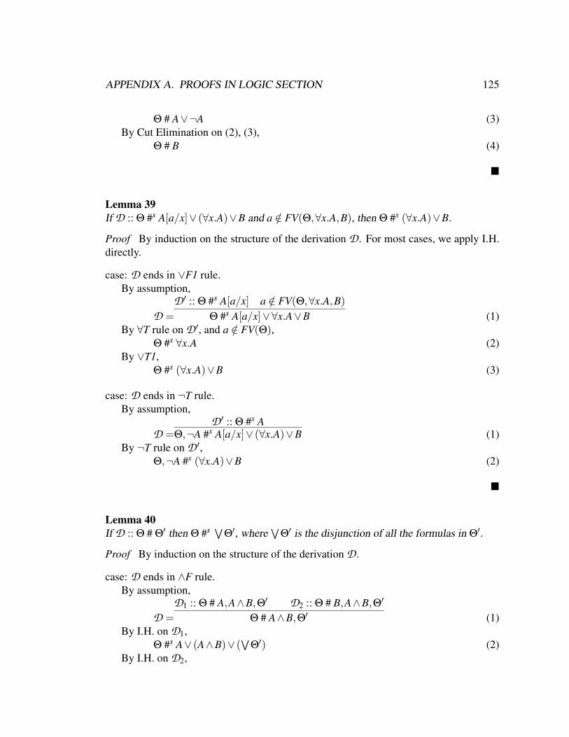
APPENDIX A. PROOFS IN LOGIC SECTION 125
Θ # A∨¬A (3)By Cut Elimination on (2), (3),
Θ # B (4)
Lemma 39If D :: Θ #s A[a/x]∨ (∀x.A)∨B and a /∈ FV(Θ,∀x.A,B), then Θ #s (∀x.A)∨B.
Proof By induction on the structure of the derivation D . For most cases, we apply I.H.directly.
case: D ends in ∨F1 rule.By assumption,
D =D ′ :: Θ #s A[a/x] a /∈ FV(Θ,∀x.A,B)
Θ #s A[a/x]∨∀x.A∨B (1)By ∀T rule on D ′, and a /∈ FV(Θ),
Θ #s ∀x.A (2)By ∨T1,
Θ #s (∀x.A)∨B (3)
case: D ends in ¬T rule.By assumption,
D =D ′ :: Θ #s A
Θ,¬A #s A[a/x]∨ (∀x.A)∨B (1)By ¬T rule on D ′,
Θ,¬A #s (∀x.A)∨B (2)
Lemma 40If D :: Θ # Θ′ then Θ #s W
Θ′, whereW
Θ′ is the disjunction of all the formulas in Θ′.
Proof By induction on the structure of the derivation D .
case: D ends in ∧F rule.By assumption,
D =D1 :: Θ # A,A∧B,Θ′ D2 :: Θ # B,A∧B,Θ′
Θ # A∧B,Θ′ (1)By I.H. on D1,
Θ #s A∨ (A∧B)∨ (W
Θ′) (2)By I.H. on D2,
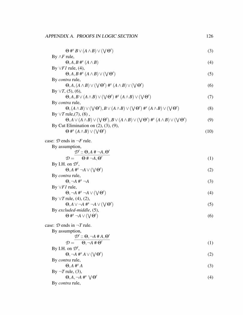
APPENDIX A. PROOFS IN LOGIC SECTION 126
Θ #s B∨ (A∧B)∨ (W
Θ′) (3)By ∧F rule,
Θ,A,B #s (A∧B) (4)By ∨F1 rule, (4),
Θ,A,B #s (A∧B)∨ (W
Θ′) (5)By contra rule,
Θ,A,(A∧B)∨ (W
Θ′) #s (A∧B)∨ (W
Θ′) (6)By ∨T, (5), (6),
Θ,A,B∨ (A∧B)∨ (W
Θ′) #s (A∧B)∨ (W
Θ′) (7)By contra rule,
Θ,(A∧B)∨ (W
Θ′),B∨ (A∧B)∨ (W
Θ′) #s (A∧B)∨ (W
Θ′) (8)By ∨T rule,(7), (8) ,
Θ,A∨ (A∧B)∨ (W
Θ′),B∨ (A∧B)∨ (W
Θ′) #s (A∧B)∨ (W
Θ′) (9)By Cut Elimination on (2), (3), (9),
Θ #s (A∧B)∨ (W
Θ′) (10)
case: D ends in ¬F rule.By assumption,
D =D ′ :: Θ,A # ¬A,Θ′
Θ # ¬A,Θ′ (1)By I.H. on D ′,
Θ,A #s ¬A∨ (W
Θ′) (2)By contra rule,
Θ,¬A #s ¬A (3)By ∨F1 rule,
Θ,¬A #s ¬A∨ (W
Θ′) (4)By ∨T rule, (4), (2),
Θ,A∨¬A #s ¬A∨ (W
Θ′) (5)By excluded-middle, (5),
Θ #s ¬A∨ (W
Θ′) (6)
case: D ends in ¬T rule.By assumption,
D =D ′ :: Θ,¬A # A,Θ′
Θ,¬A # Θ′ (1)By I.H. on D ′,
Θ,¬A #s A∨ (W
Θ′) (2)By contra rule,
Θ,A #s A (3)By ¬T rule, (3),
Θ,A,¬A #s WΘ′ (4)
By contra rule,
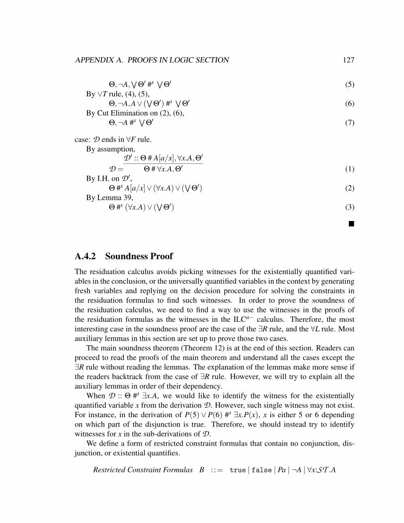
APPENDIX A. PROOFS IN LOGIC SECTION 127
Θ,¬A,W
Θ′ #s WΘ′ (5)
By ∨T rule, (4), (5),Θ,¬A,A∨ (
WΘ′) #s W
Θ′ (6)By Cut Elimination on (2), (6),
Θ,¬A #s WΘ′ (7)
case: D ends in ∀F rule.By assumption,
D =D ′ :: Θ # A[a/x],∀x.A,Θ′
Θ # ∀x.A,Θ′ (1)By I.H. on D ′,
Θ #s A[a/x]∨ (∀x.A)∨ (W
Θ′) (2)By Lemma 39,
Θ #s (∀x.A)∨ (W
Θ′) (3)
A.4.2 Soundness ProofThe residuation calculus avoids picking witnesses for the existentially quantified vari-ables in the conclusion, or the universally quantified variables in the context by generatingfresh variables and replying on the decision procedure for solving the constraints inthe residuation formulas to find such witnesses. In order to prove the soundness ofthe residuation calculus, we need to find a way to use the witnesses in the proofs ofthe residuation formulas as the witnesses in the ILCa− calculus. Therefore, the mostinteresting case in the soundness proof are the case of the ∃R rule, and the ∀L rule. Mostauxiliary lemmas in this section are set up to prove those two cases.
The main soundness theorem (Theorem 12) is at the end of this section. Readers canproceed to read the proofs of the main theorem and understand all the cases except the∃R rule without reading the lemmas. The explanation of the lemmas make more sense ifthe readers backtrack from the case of ∃R rule. However, we will try to explain all theauxiliary lemmas in order of their dependency.
When D :: Θ #s ∃x.A, we would like to identify the witness for the existentiallyquantified variable x from the derivation D . However, such single witness may not exist.For instance, in the derivation of P(5)∨P(6) #s ∃x.P(x), x is either 5 or 6 dependingon which part of the disjunction is true. Therefore, we should instead try to identifywitnesses for x in the sub-derivations of D .
We define a form of restricted constraint formulas that contain no conjunction, dis-junction, or existential quantifies.
Restricted Constraint Formulas B : := true | false | Pa | ¬A | ∀x:ST .A

APPENDIX A. PROOFS IN LOGIC SECTION 128
We define two kinds of transformation of a context to a set of contexts: Θ 7−→ S,Θ 7−→† S. The definitions are as follows.
Θ,A1∧A2 7−→ (Θ,A1,A2)Θ,A1∨A2 7−→ (Θ,A1),(Θ,A2)Θ,∃x:ST .A 7−→ (Θ,A[a/x]) a is freshΘ,∀x:ST .A 7−→† (Θ,A[t/x])Θ 7−→† (Θ,A),(Θ,¬A)
Intuitively, a context transforms to the set of contexts that are the contexts in thepremises of the left rule of the connective being decomposed.
We define the transformation of the set of contexts based on the transformation ofindividual context in the set.
Θ 7−→ S1S∪Θ 7−→ S∪S1
Θ 7−→ S1 or Θ 7−→† S1
S∪Θ 7−→† S∪S1
Lemma 41If Θ #s ∀x.A then Θ #s A[a/x] and a /∈ FV(Θ).
The following two lemmas state that the transformation 7−→ preserves provability.
Lemma 42If Θ #s A and Θ 7−→ S then for all Θi ∈ S, Θi #s A
Proof By examine the definition of Θ 7−→ S, we need to prove the following:
1. If D :: Θ,A1∧A2 #s B then Θ,A1,A2 #s B.
2. If D :: Θ,A1∨A2 #s B then Θ,A1 #s B, and Θ,A2 #s B.
3. If D :: Θ,∃x.A #s B then Θ,A[a/x] #s B.
1. By induction on the structure of D .
case: D ends in contra rule.By assumption,
Θ,A1∧A2 #s A1∧A2 (1)By contra rule,
Θ,A1 #s A1 (2)Θ,A2 #s A2 (3)
By ∧F rule,Θ,A1,A2 #s A1∧A2 (4)
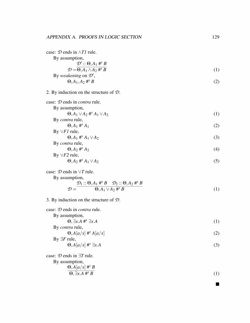
APPENDIX A. PROOFS IN LOGIC SECTION 129
case: D ends in ∧T1 rule.By assumption,
D =D ′ :: Θ,A1 #s BΘ,A1∧A2 #s B (1)
By weakening on D ′,Θ,A1,A2 #s B (2)
2. By induction on the structure of D .
case: D ends in contra rule.By assumption,
Θ,A1∨A2 #s A1∨A2 (1)By contra rule,
Θ,A1 #s A1 (2)By ∨F1 rule,
Θ,A1 #s A1∨A2 (3)By contra rule,
Θ,A2 #s A2 (4)By ∨F2 rule,
Θ,A2 #s A1∨A2 (5)
case: D ends in ∨T rule.By assumption,
D =D1 :: Θ,A1 #s B D2 :: Θ,A2 #s B
Θ,A1∨A2 #s B (1)
3. By induction on the structure of D .
case: D ends in contra rule.By assumption,
Θ,∃x.A #s ∃x.A (1)By contra rule,
Θ,A[a/x] #s A[a/x] (2)By ∃F rule,
Θ,A[a/x] #s ∃x.A (3)
case: D ends in ∃T rule.By assumption,
Θ,A[a/x] #s BΘ,∃x.A #s B (1)

APPENDIX A. PROOFS IN LOGIC SECTION 130
Lemma 43If for all Θ ∈ S, Θ #s A and S 7−→∗ S′ then for all Θi ∈ S′, Θi #s A.
Proof By induction on the number of steps n in Θ 7−→n S.
case: n = 0 trivial
case: Assume when n = k (k ≥ 0) the conclusion holds,now we consider n = k +1
By assumption,S 7−→ S1 7−→k Sk+1 (1)∀Θ ∈ S,Θ #s A (2)
By definition of S 7−→ S1,S = S′∪Θ 7−→ S′∪S2 where Θ 7−→ S2 (3)and S′∪S2 = S1 (4)
By Lemma 42, (3),∀Θi ∈ S2,Θi #s A (5)
By (5), (2), (3),∀Θn ∈ S′∪S2,Θn #s A (6)
By I.H. on k (4), (1),∀Θi ∈ Sk+1,Θi #s A (7)
Now we prove that when Θ #s ∃x.A, Θ can be transformed into a set of contexts S,and there exists some ti for each context Θi in S such that Θi entails A[ti/x].
Lemma 441. If Θ #s ∃x.A, then exists S, S′ such that Θ 7−→∗ S 7−→† ∗ S′, all the formulas in S
have the restricted form, and ∀Θi ∈ S′, there exists a term ti such that Θi #s A[ti/x].
2. If Θ #s ∃x.A, and all the formulas in Θ have the restricted form, then exists S suchthat Θ 7−→† ∗ S, and ∀Θi ∈ S, there exists a term ti such that Θi #s A[ti/x].
Proof 1. Use 2 directly.
By assumption,Θ #s ∃x.A (1)
By examine the definition of Θ 7−→ S, and S 7−→ S′,there exists a S such that Θ 7−→∗ S (2)and ∀Θi ∈ S, all the formulas in Θi have the restricted form (3)
By Lemma 43, (1), (2),∀Θi ∈ S,Θi #s ∃x.A (4)
By Apply 2 on (3), (4),
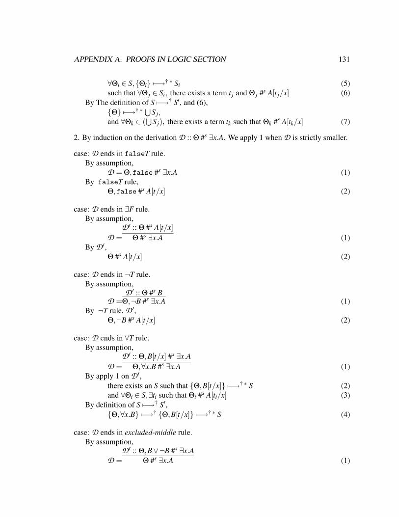
APPENDIX A. PROOFS IN LOGIC SECTION 131
∀Θi ∈ S,Θi 7−→† ∗ Si (5)such that ∀Θ j ∈ Si, there exists a term t j and Θ j #s A[t j/x] (6)
By The definition of S 7−→† S′, and (6),Θ 7−→† ∗ S
S j,and ∀Θk ∈ (
SS j), there exists a term tk such that Θk #s A[tk/x] (7)
2. By induction on the derivation D :: Θ #s ∃x.A. We apply 1 when D is strictly smaller.
case: D ends in falseT rule.By assumption,
D = Θ,false #s ∃x.A (1)By falseT rule,
Θ,false #s A[t/x] (2)
case: D ends in ∃F rule.By assumption,
D =D ′ :: Θ #s A[t/x]
Θ #s ∃x.A (1)By D ′,
Θ #s A[t/x] (2)
case: D ends in ¬T rule.By assumption,
D =D ′ :: Θ #s B
Θ,¬B #s ∃x.A (1)By ¬T rule, D ′,
Θ,¬B #s A[t/x] (2)
case: D ends in ∀T rule.By assumption,
D =D ′ :: Θ,B[t/x] #s ∃x.A
Θ,∀x.B #s ∃x.A (1)By apply 1 on D ′,
there exists an S such that Θ,B[t/x] 7−→† ∗ S (2)and ∀Θi ∈ S,∃ti such that Θi #s A[ti/x] (3)
By definition of S 7−→† S′,Θ,∀x.B 7−→† Θ,B[t/x] 7−→† ∗ S (4)
case: D ends in excluded-middle rule.By assumption,
D =D ′ :: Θ,B∨¬B #s ∃x.A
Θ #s ∃x.A (1)
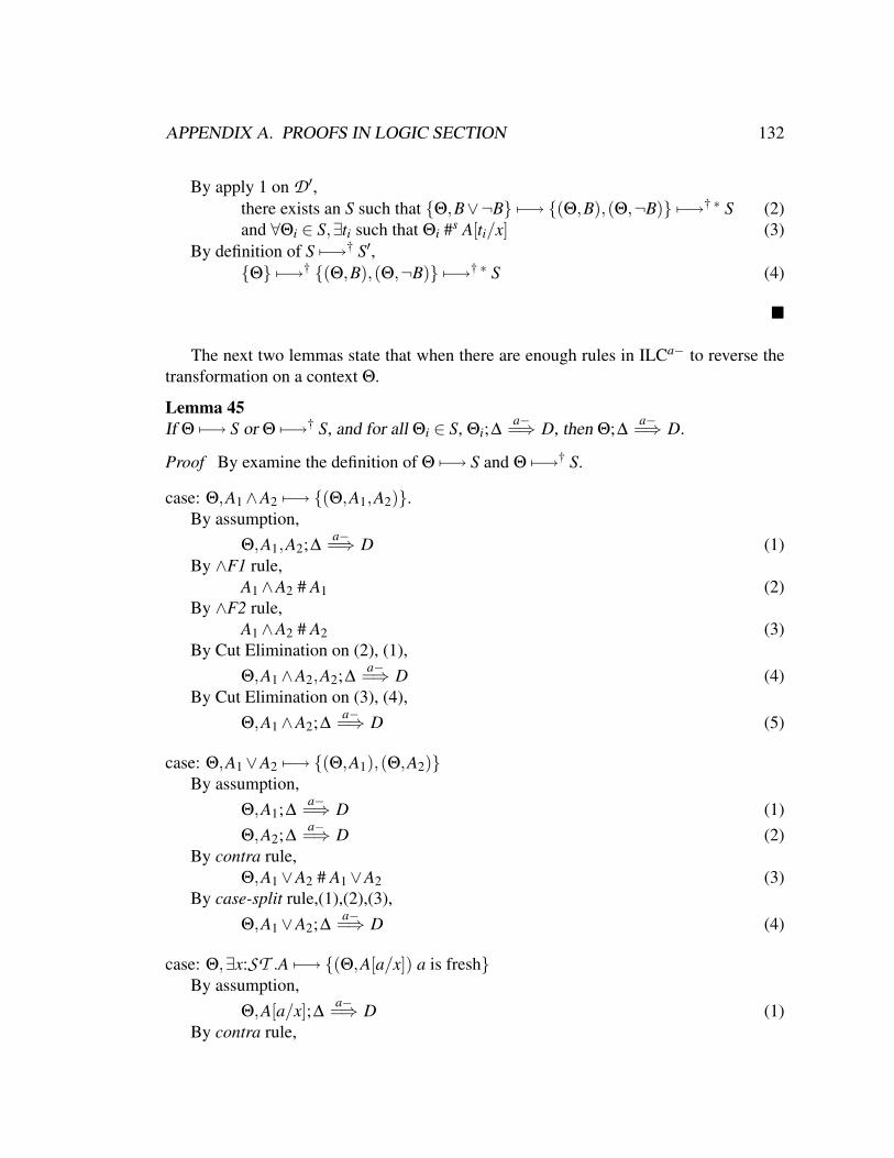
APPENDIX A. PROOFS IN LOGIC SECTION 132
By apply 1 on D ′,there exists an S such that Θ,B∨¬B 7−→ (Θ,B),(Θ,¬B) 7−→† ∗ S (2)and ∀Θi ∈ S,∃ti such that Θi #s A[ti/x] (3)
By definition of S 7−→† S′,Θ 7−→† (Θ,B),(Θ,¬B) 7−→† ∗ S (4)
The next two lemmas state that when there are enough rules in ILCa− to reverse thetransformation on a context Θ.
Lemma 45If Θ 7−→ S or Θ 7−→† S, and for all Θi ∈ S, Θi;∆
a−=⇒ D, then Θ;∆a−=⇒ D.
Proof By examine the definition of Θ 7−→ S and Θ 7−→† S.
case: Θ,A1∧A2 7−→ (Θ,A1,A2).By assumption,
Θ,A1,A2;∆a−=⇒ D (1)
By ∧F1 rule,A1∧A2 # A1 (2)
By ∧F2 rule,A1∧A2 # A2 (3)
By Cut Elimination on (2), (1),Θ,A1∧A2,A2;∆
a−=⇒ D (4)By Cut Elimination on (3), (4),
Θ,A1∧A2;∆a−=⇒ D (5)
case: Θ,A1∨A2 7−→ (Θ,A1),(Θ,A2)By assumption,
Θ,A1;∆a−=⇒ D (1)
Θ,A2;∆a−=⇒ D (2)
By contra rule,Θ,A1∨A2 # A1∨A2 (3)
By case-split rule,(1),(2),(3),Θ,A1∨A2;∆
a−=⇒ D (4)
case: Θ,∃x:ST .A 7−→ (Θ,A[a/x]) a is freshBy assumption,
Θ,A[a/x];∆a−=⇒ D (1)
By contra rule,

APPENDIX A. PROOFS IN LOGIC SECTION 133
Θ,∃x.A # ∃x.A (2)By ∃T rule, (1), (2),
Θ,∃x.A;∆a−=⇒ D (3)
case: Θ,∀x:ST .A 7−→† (Θ,A[t/x])By assumption,
Θ,A[t/x];∆a−=⇒ D (1)
By contra rule,Θ,A[t/x] # A[t/x] (2)
By ∀F rule,Θ,∀x.A # A[t/x] (3)
By Cut Elimination on (1), (3),Θ,∀x.A;∆
a−=⇒ D (4)
case: Θ 7−→† (Θ,A),(Θ,¬A)By assumption,
Θ,A;∆a−=⇒ D (1)
Θ,¬A;∆a−=⇒ D (2)
By contra rule,Θ,A∨¬A # A∨¬A (3)
By Lemma 37,Θ # A∨¬A (4)
By case-split rule, (1). (2), (4),Θ;∆
a−=⇒ D (5)
Lemma 46If Θ 7−→† ∗ S, and ∀Θi ∈ S, Θi;∆
a−=⇒ D, then Θ;∆a−=⇒ D.
Proof By induction on the number of steps n in Θ 7−→n S.
case: n = 0 trivial
case: Assume when n = k (k ≥ 0) the conclusion holds, now we consider n = k +1By assumption,
Θ 7−→† k Sk 7−→† Sk+1 (1)∀Θ j ∈ Sk+1,Θ j;∆
a−=⇒ D (2)By definition of S 7−→† S′,
Sk = S′k∪Θ1 7−→ S′k∪S1 where Θ1 7−→ S1 or Θ1 7−→† S1 (3)
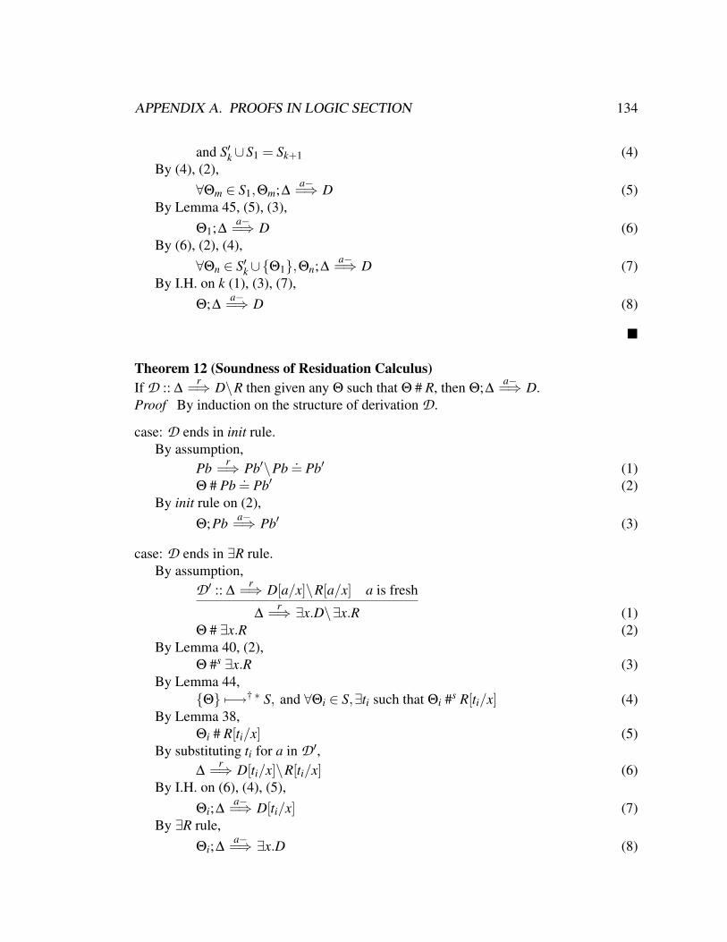
APPENDIX A. PROOFS IN LOGIC SECTION 134
and S′k∪S1 = Sk+1 (4)By (4), (2),
∀Θm ∈ S1,Θm;∆a−=⇒ D (5)
By Lemma 45, (5), (3),Θ1;∆
a−=⇒ D (6)By (6), (2), (4),
∀Θn ∈ S′k∪Θ1,Θn;∆a−=⇒ D (7)
By I.H. on k (1), (3), (7),Θ;∆
a−=⇒ D (8)
Theorem 12 (Soundness of Residuation Calculus)If D :: ∆
r=⇒ D\R then given any Θ such that Θ # R, then Θ;∆a−=⇒ D.
Proof By induction on the structure of derivation D .
case: D ends in init rule.By assumption,
Pb r=⇒ Pb′\Pb .= Pb′ (1)Θ # Pb .= Pb′ (2)
By init rule on (2),Θ;Pb a−=⇒ Pb′ (3)
case: D ends in ∃R rule.By assumption,
D ′ :: ∆r=⇒ D[a/x]\R[a/x] a is fresh
∆r=⇒ ∃x.D\∃x.R (1)
Θ # ∃x.R (2)By Lemma 40, (2),
Θ #s ∃x.R (3)By Lemma 44,
Θ 7−→† ∗ S, and ∀Θi ∈ S,∃ti such that Θi #s R[ti/x] (4)By Lemma 38,
Θi # R[ti/x] (5)By substituting ti for a in D ′,
∆r=⇒ D[ti/x]\R[ti/x] (6)
By I.H. on (6), (4), (5),Θi;∆
a−=⇒ D[ti/x] (7)By ∃R rule,
Θi;∆a−=⇒ ∃x.D (8)
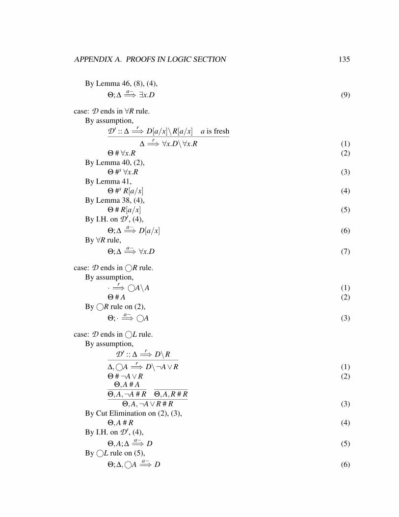
APPENDIX A. PROOFS IN LOGIC SECTION 135
By Lemma 46, (8), (4),Θ;∆
a−=⇒ ∃x.D (9)
case: D ends in ∀R rule.By assumption,
D ′ :: ∆r=⇒ D[a/x]\R[a/x] a is fresh
∆r=⇒ ∀x.D\∀x.R (1)
Θ # ∀x.R (2)By Lemma 40, (2),
Θ #s ∀x.R (3)By Lemma 41,
Θ #s R[a/x] (4)By Lemma 38, (4),
Θ # R[a/x] (5)By I.H. on D ′, (4),
Θ;∆a−=⇒ D[a/x] (6)
By ∀R rule,Θ;∆
a−=⇒ ∀x.D (7)
case: D ends in ©R rule.By assumption,
· r=⇒ ©A\A (1)Θ # A (2)
By ©R rule on (2),Θ; · a−=⇒ ©A (3)
case: D ends in ©L rule.By assumption,
D ′ :: ∆r=⇒ D\R
∆,©A r=⇒ D\¬A∨R (1)Θ # ¬A∨R (2)
Θ,A # AΘ,A,¬A # R Θ,A,R # R
Θ,A,¬A∨R # R (3)By Cut Elimination on (2), (3),
Θ,A # R (4)By I.H. on D ′, (4),
Θ,A;∆a−=⇒ D (5)
By ©L rule on (5),Θ;∆,©A a−=⇒ D (6)
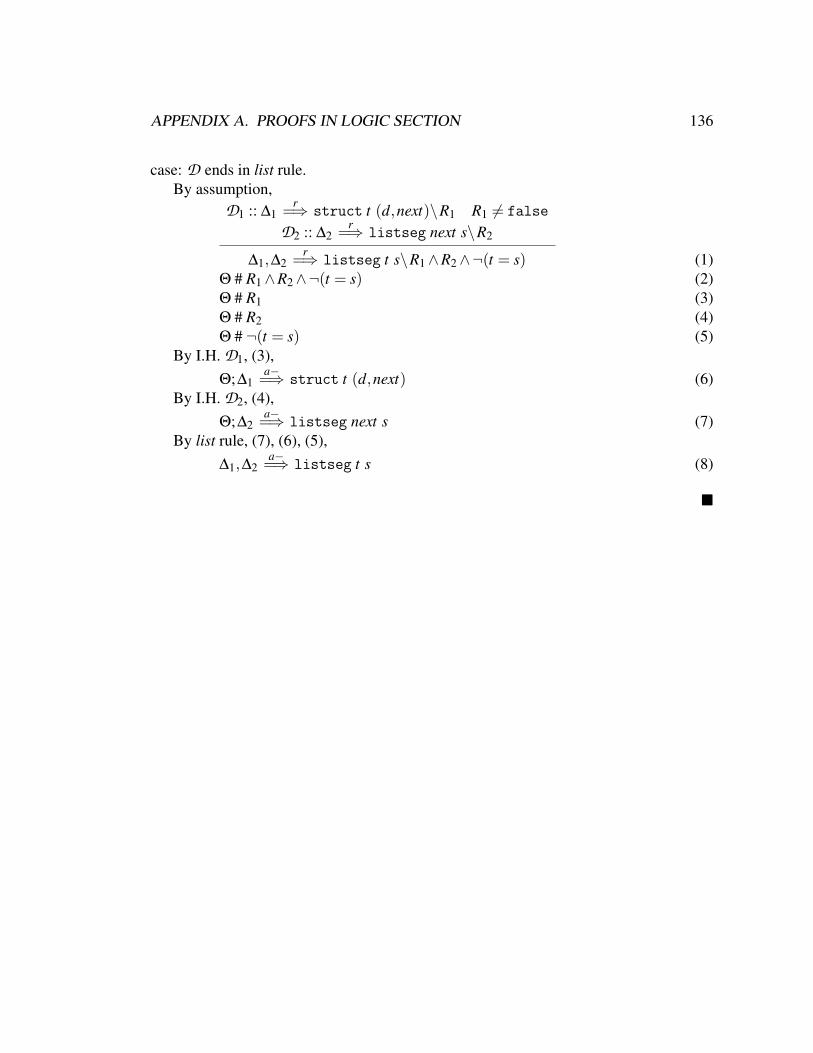
APPENDIX A. PROOFS IN LOGIC SECTION 136
case: D ends in list rule.By assumption,
D1 :: ∆1r=⇒ struct t (d,next)\R1 R1 6= false
D2 :: ∆2r=⇒ listseg next s\R2
∆1,∆2r=⇒ listseg t s\R1∧R2∧¬(t = s) (1)
Θ # R1∧R2∧¬(t = s) (2)Θ # R1 (3)Θ # R2 (4)Θ # ¬(t = s) (5)
By I.H. D1, (3),Θ;∆1
a−=⇒ struct t (d,next) (6)By I.H. D2, (4),
Θ;∆2a−=⇒ listseg next s (7)
By list rule, (7), (6), (5),∆1,∆2
a−=⇒ listseg t s (8)
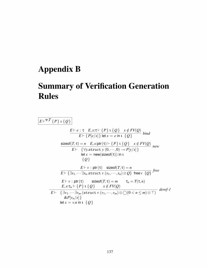
Appendix B
Summary of Verification GenerationRules
E `Ψ;T P s Q
E ` e : τ E,x:τ ` P ι Q x /∈ FV(Q)E ` P[e/x] let x = e in ι Q bind
sizeof(T,τ) = n E,x:ptr(τ) ` P ι Q x /∈ FV(Q)E ` ∀y.struct y (0, · · · ,0) ( P[y/x]
let x = new(sizeof(τ)) in ι
Q
new
E ` v : ptr(τ) sizeof(T,τ) = nE ` ∃x1. · · ·∃xn.struct v (x1, · · · ,xn)⊗Q freev Q free
E ` v : ptr(τ) sizeof(T,τ) = m τn = T(τ,n)E,x:τn ` P ι Q x /∈ FV(Q)
E ` ∃v1. · · ·∃vm.(struct v (v1, · · · ,vm)⊗©(0 < n≤ m)⊗>)&P[vn/x]
let x = v.n in ι Q
deref-1
137

APPENDIX B. SUMMARY OF VERIFICATION GENERATION RULES 138
E ` v : list τi = T(node,n) E,x:τi ` P ι Q x /∈ FV(Q)E ` ∃y.∀v1.∀v2.listseg v y⊗©(¬(v = y))⊗©(0 < n≤ 2)
⊗((struct v (v1,v2)⊗listseg v2 y) ( P[vn/x])let x = v.n in ι Q
deref-2
E ` v : ptr(τ) sizeof(T,τ) = mE ` ∃v1. · · ·∃vm.struct v (v1, · · · ,vm)⊗©(0 < n≤ m)
⊗ (struct v (v1, · · · ,vn−1,e1,vn+1, · · ·vm) ( Q)v.n := e1 Q
assignment-1
E ` v : list
v′1 = e1,v′2 = v2 i f n = 1v′1 = v1,v′2 = e1 i f n = 2
E ` c∃y.∀v1.∀v2.listseg v y⊗©(¬(v = y))⊗©(0 < n≤ 2)⊗ ((struct v (v′1,v
′2)⊗listseg v′2 y) ( Q)
v.n := e1 Q
assignment-2
E ` P s P′ E ` P′ ι QE ` P s ; ι Q Seq
E ` P1 s1 Q E ` P2 s2 QE ` (©B ( P1)&(©¬B ( P2) if B then s1 else s2 Q if
E′ = var typing(R) dom(E′)∩FV(I) = /0 dom(E′)∩FV(Q) = /0
E,E′ ` P s I E ` Fρ R
E ` F[ρ((©¬B ( Q)&(©B ( P))]⊗!(I ( F[ρ((©¬B ( Q)&(©B ( P))]) while[I] R do s Q
while
E,x:τ f ` P s Q x /∈ FV(Q)Ψ( f ) = (a:τa ):τ f fb [E f ]Pre∀ret.Post ∆ = dom(E f )
E ` ∃∆.Pre[e/a]⊗ (∀ret.Post[e/a] ( P[ret/x])let x = f (e) in s Q
fun call
E ` Q[e/ret] returne ∀ret.Q return

Appendix C
Proofs for the Soundness of VCGen
Lemma 17 If ` ΨOK, E `Ψ,T P s Q then for all substitution σ for variables indom(E), for all n≥ 0, n σ(P) σ(s) σ(Q) with regard to Ψ.Proof By induction on n, call upon Lemma 47, Lemma 18.
case: n = 0, the conclusion holds.
case: assume for all n, 0≤ n≤ m the conclusion holds,now examine the case where n = m+1. We do induction on the structure of s.
subcase: s = let x = e in s′
By assumption,E ` e : τ E,x:τ ` P s′ Q x /∈ FV(Q)
E ` P[e/x] let x = e in s′ Q (1)σ is a substitution for all the variables in dom(E) (2)H σ(P[e/x]) (3)H σ′(P) where σ′ = (σ,Jσ(e)K/x) (4)
By Operational semantics,(K;H]H1;σ(let x = e in s′ )) 7−→ (K;H]H1;σ(s′)[Jσ(e)K/x]) (5)
By I.H. on n−1, s′, and x /∈ FV(Q),n−1 σ′(P) σ′(s′) σ(Q) (6)
By (5), (6), and the definition of k P s Q,n σ(P) σ(s) σ(Q) (7)
subcase: s = let x = new(sizeof(τ)) in s′
By assumption,sizeof(T,τ) = n E,x:ptrτ ` P s′ Q
x /∈ FV(Q) where es = (0, · · ·0)
E ` ∀y.struct y es ( P[y/x]let x = new(sizeof(τ)) in s′ Q (1)
139
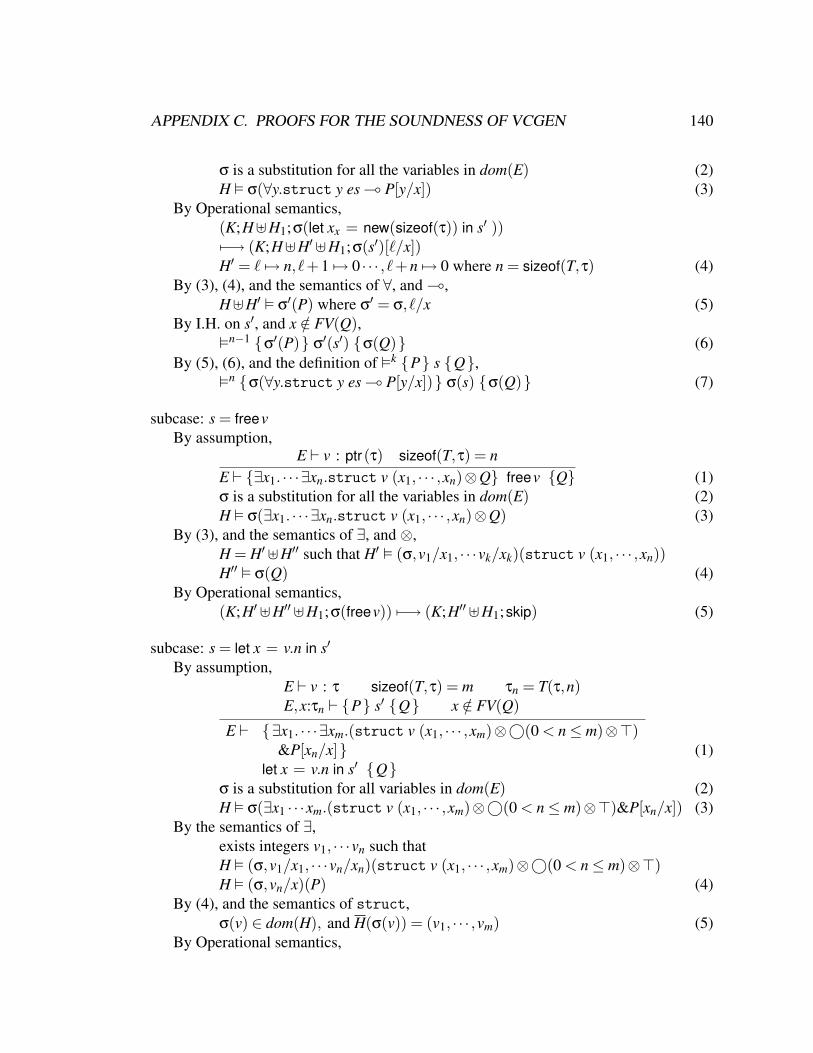
APPENDIX C. PROOFS FOR THE SOUNDNESS OF VCGEN 140
σ is a substitution for all the variables in dom(E) (2)H σ(∀y.struct y es ( P[y/x]) (3)
By Operational semantics,(K;H]H1;σ(let xx = new(sizeof(τ)) in s′ ))7−→ (K;H]H′]H1;σ(s′)[`/x])H′ = ` 7→ n, `+1 7→ 0 · · · , `+n 7→ 0 where n = sizeof(T,τ) (4)
By (3), (4), and the semantics of ∀, and (,H]H′ σ′(P) where σ′ = σ, `/x (5)
By I.H. on s′, and x /∈ FV(Q),n−1 σ′(P) σ′(s′) σ(Q) (6)
By (5), (6), and the definition of k P s Q,n σ(∀y.struct y es ( P[y/x]) σ(s) σ(Q) (7)
subcase: s = freevBy assumption,
E ` v : ptr(τ) sizeof(T,τ) = nE ` ∃x1. · · ·∃xn.struct v (x1, · · · ,xn)⊗Q freev Q (1)σ is a substitution for all the variables in dom(E) (2)H σ(∃x1. · · ·∃xn.struct v (x1, · · · ,xn)⊗Q) (3)
By (3), and the semantics of ∃, and ⊗,H = H′]H′′ such that H′ (σ,v1/x1, · · ·vk/xk)(struct v (x1, · · · ,xn))H′′ σ(Q) (4)
By Operational semantics,(K;H′]H′′]H1;σ(freev)) 7−→ (K;H′′]H1;skip) (5)
subcase: s = let x = v.n in s′
By assumption,E ` v : τ sizeof(T,τ) = m τn = T(τ,n)E,x:τn ` P s′ Q x /∈ FV(Q)
E ` ∃x1. · · ·∃xm.(struct v (x1, · · · ,xm)⊗©(0 < n≤ m)⊗>)&P[xn/x]
let x = v.n in s′ Q(1)
σ is a substitution for all variables in dom(E) (2)H σ(∃x1 · · ·xm.(struct v (x1, · · · ,xm)⊗©(0 < n≤ m)⊗>)&P[xn/x]) (3)
By the semantics of ∃,exists integers v1, · · ·vn such thatH (σ,v1/x1, · · ·vn/xn)(struct v (x1, · · · ,xm)⊗©(0 < n≤ m)⊗>)H (σ,vn/x)(P) (4)
By (4), and the semantics of struct,σ(v) ∈ dom(H), and H(σ(v)) = (v1, · · · ,vm) (5)
By Operational semantics,
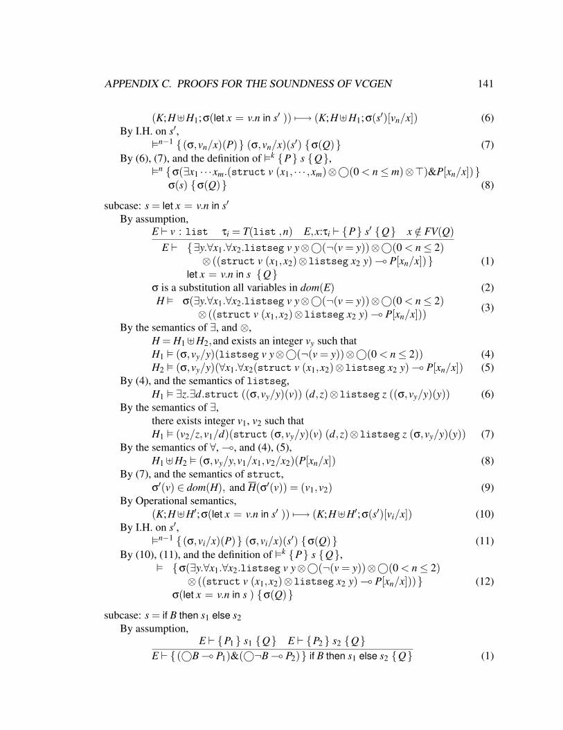
APPENDIX C. PROOFS FOR THE SOUNDNESS OF VCGEN 141
(K;H]H1;σ(let x = v.n in s′ )) 7−→ (K;H]H1;σ(s′)[vn/x]) (6)By I.H. on s′,
n−1 (σ,vn/x)(P) (σ,vn/x)(s′) σ(Q) (7)By (6), (7), and the definition of k P s Q,
n σ(∃x1 · · ·xm.(struct v (x1, · · · ,xm)⊗©(0 < n≤ m)⊗>)&P[xn/x])σ(s) σ(Q) (8)
subcase: s = let x = v.n in s′
By assumption,E ` v : list τi = T(list ,n) E,x:τi ` P s′ Q x /∈ FV(Q)
E ` ∃y.∀x1.∀x2.listseg v y⊗©(¬(v = y))⊗©(0 < n≤ 2)⊗ ((struct v (x1,x2)⊗listseg x2 y) ( P[xn/x])
let x = v.n in s Q(1)
σ is a substitution all variables in dom(E) (2)H σ(∃y.∀x1.∀x2.listseg v y⊗©(¬(v = y))⊗©(0 < n≤ 2)
⊗ ((struct v (x1,x2)⊗listseg x2 y) ( P[xn/x])) (3)
By the semantics of ∃, and ⊗,H = H1]H2,and exists an integer vy such thatH1 (σ,vy/y)(listseg v y⊗©(¬(v = y))⊗©(0 < n≤ 2)) (4)H2 (σ,vy/y)(∀x1.∀x2(struct v (x1,x2)⊗listseg x2 y) ( P[xn/x]) (5)
By (4), and the semantics of listseg,H1 ∃z.∃d.struct ((σ,vy/y)(v)) (d,z)⊗listseg z ((σ,vy/y)(y)) (6)
By the semantics of ∃,there exists integer v1, v2 such thatH1 (v2/z,v1/d)(struct (σ,vy/y)(v) (d,z)⊗listseg z (σ,vy/y)(y)) (7)
By the semantics of ∀, (, and (4), (5),H1]H2 (σ,vy/y,v1/x1,v2/x2)(P[xn/x]) (8)
By (7), and the semantics of struct,σ′(v) ∈ dom(H), and H(σ′(v)) = (v1,v2) (9)
By Operational semantics,(K;H]H′;σ(let x = v.n in s′ )) 7−→ (K;H]H′;σ(s′)[vi/x]) (10)
By I.H. on s′,n−1 (σ,vi/x)(P) (σ,vi/x)(s′) σ(Q) (11)
By (10), (11), and the definition of k P s Q, σ(∃y.∀x1.∀x2.listseg v y⊗©(¬(v = y))⊗©(0 < n≤ 2)
⊗ ((struct v (x1,x2)⊗listseg x2 y) ( P[xn/x]))σ(let x = v.n in s ) σ(Q)
(12)
subcase: s = if B then s1 else s2By assumption,
E ` P1 s1 Q E ` P2 s2 QE ` (©B ( P1)&(©¬B ( P2) if B then s1 else s2 Q (1)
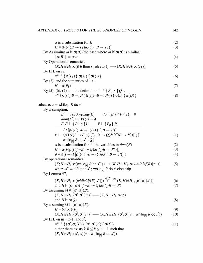
APPENDIX C. PROOFS FOR THE SOUNDNESS OF VCGEN 142
σ is a substitution for E (2)H σ((©B ( P1)&(©¬B ( P2)) (3)
By Assuming M σ(B) (the case where M 2 σ(B) is similar),Jσ(B)K = true (4)
By Operational semantics,(K;H]H1;σ(if B then s1 else s2)) 7−→ (K;H]H1;σ(s1)) (5)
By I.H. on s1,n−1 σ(P1) σ(s1) σ(Q) (6)
By (3), and the semantics of (,H σ(P1) (7)
By (5), (6), (7) and the definition of k P s Q,n σ((©B ( P1)&(©¬B ( P2)) σ(s) σ(Q) (8)
subcase: s = while[I] R do s′
By assumption,E′ = var typing(R) dom(E′)∩FV(I) = /0
dom(E′)∩FV(Q) = /0
E,E′ ` P s I E ` Fρ R
E `F[ρ((©¬B ( Q)&(©B ( P))]⊗(1&(I ( F[ρ((©¬B ( Q)&(©B ( P))]))while[I] R do s′ Q
(1)
σ is a substitution for all the variables in dom(E) (2)H σ(F[ρ((©¬B ( Q)&(©B ( P))]) (3)/0 σ(I ( F[ρ((©¬B ( Q)&(©B ( P))]) (4)
By operational semantics,(K;H]H1;σ(while[I] R do s′)) 7−→ (K,H]H1,σ(while2if(R)[s′′])) (5)where s′′ = if B then s′ ; while[I] R do s′ else skip
By Lemma 47,
(K,H]H1,σ(while2if(R)[s′′]))Ψ,T n17−→ (K,H]H1,(σ′,σ)(s′′)) (6)
and H (σ′,σ)(©¬B ( Q)&(©B ( P) (7)By assuming M 2 (σ′,σ)(B),
(K,H]H1,(σ′,σ)(s′′)) 7−→ (K,H]H1,skip)and H σ(Q) (8)
By assuming M (σ′,σ)(B),H (σ′,σ)(P) (9)(K,H]H1,(σ′,σ)(s′′)) 7−→ (K,H]H1,(σ′,σ)(s′ ; while[I] R do s′)) (10)
By I.H. on m = n-1, and s′,n−1 (σ′,σ)(P) (σ′,σ)(s′) σ(I) (11)either there exists k,0≤ k ≤ n−1 such that(K,H]H1,(σ′,σ)(s′ ; while[I] R do s′))

APPENDIX C. PROOFS FOR THE SOUNDNESS OF VCGEN 143
Ψ,T k7−→ (K,H′]H1,skip ; σ(while[I] R do s′)), (12)and H′ σ(I) (13)or there exists K′,H′,and ι,
and (K,H]H1,(σ′,σ)(s′ ; while[I] R do s′))Ψ,T n−17−→ (K′,H′, ι) (14)
By operational Semantics,(K,H′]H1,skip ; σ(while[I] R do s′))7−→ (K,H′]H1,σ(while[I] R do s′)) (15)
By semantics of formula, and (13), (4),H′ (σ(F[ρ((©¬B ( Q)&(©B ( P))])) (16)
By semantics of formula, and (4), (16),H′ σ(F[ρ((©¬B ( Q)&(©B ( P))])
⊗1&(I ( F[ρ((©¬B ( Q)&(©B ( P))]) (17)By I.H. on n-k-1,
n−k−1 Pw σ(while[I] R do s′) σ(Q) (18)where Pw = σ(F[ρ((©¬B ( Q)&(©B ( P))])
⊗1&(I ( F[ρ((©¬B ( Q)&(©B ( P))])By (8) (10) (14) (12) (15) (18),
n Pw σ(s) σ(Q) (19)
subcase: s = let x = f (e) in s′
By assumption,E,x:τ f ` P s′ Q x /∈ FV(Q)Ψ( f ) = (a:τa ):τ f fb [E f ]Pre∀ret.Post ∆ = dom(E f )
E ` ∃E f .Pre[e/a]⊗ (∀ret.Post[e/a] ( P[ret/x])let x = f (e) in s′ Q (1)
H σ(∃E f .Pre[e/a]⊗ (∀ret.Post[e/a] ( P[ret/x])) (2)By the semantics of formulas,
exists substitution σ f for variables in dom(E f ) such thatH = Hp]Hq (3)Hp (σ,σ f )(Pre[e/a]) (4)Hq (σ,σ f )(∀ret.Post[e/a] ( P[ret/x]) (5)
By operational semantics,(K,H]H1,σ(let x = f (e) in s′ ))7−→ (let x = [ ] in σ(s′) .K,H]H1, fb[Jσ(e)K/a]) (6)
By the definition of `ΨOK,E f ,a `Ψ Pre fb ∀ret.Post (7)
By Lemma 18, (7), (4),either there exists k,0≤ k ≤ n such that(let x = [ ] in σ(s′) .K,Hp]Hq]H1,(σ,J(σ(e))K/a)fb)Ψ,T k7−→ (let x = [ ] in σ(s′) .K,H′
p]Hq]H1, returne1) (8)

APPENDIX C. PROOFS FOR THE SOUNDNESS OF VCGEN 144
and H′p (σ,σ f ,σ(e)/a)(Post)[Je1 K/ret] (9)
or there exists K′,H′, and ι,
and (let x = [ ] in . K,Hp]Hq]H1, fb)Ψ,T n7−→ (K′,H′, ι) (10)
By (5), (9),and the semantics of formulas,H′
p]Hq σ(P)[Je1 K/x] (11)By operational semantics,
(let x = [ ] in σ(s′) .K,H′p]Hq]H1, returne1)
7−→ (K,H′p]Hq]H1,σ(s′)[Je1 K/x]) (12)
By I.H. on n− k−1 and s′,n−k−1 (σ,Je1 K/x)(P) σ(s′) σ(Q) (13)
By (10), (8), (12), (13) ,n σ(∃E f .Pre[e/a]⊗ (∀ret.Post[e/a] ( P[ret/x]) σ(s) σ(Q) (14)
Lemma 47if E ` Fρ R, and while2if(R) = sB, σ is a substitution for variables in dom(E), and
H σ(F[ρ(P)]), then (K,H]H1,σ(sB[s′]))Ψ,T n7−→ (K,H′]H1,(σ′,σ)(s′))), such that H′
(σ′,σ)(P)).
Proof By induction on the structure of R.
case: R = BBy assumption,
· ` [ ]· B (1)while2if(R) = [ ]B (2)H P (3)the conclusion holds for n = 0 (4)
case: R = let x = y.k in R′
By assumption,E,x:τk ` Fρ R′ E ` y : ptrτ sizeof(T,τ) = n T (τ,k) = τk
E ` ∃x1. · · ·∃xn.(struct y (x1, · · · ,xn)⊗©(0 < k ≤ n)⊗>)&Fρ[xk/x]
let x = y.k in R′(1)
while2if(R′) = sB
while2if(let x = y.k in R′ ) = let x = y.k in sB (2)H σ(∃x1. · · ·∃xn.(struct y (x1, · · · ,xn)⊗©(0 < n≤ n)⊗>)
&F[ρ(P)][xk/x]) (3)
APPENDIX C. PROOFS FOR THE SOUNDNESS OF VCGEN 145
By the semantics of formulas, there exists values v1, and v2 such that,H struct σ(y) (v1,v2)⊗©(0 < k ≤ 2)⊗> (4)H (vk/x,σ)(F[ρ(P)]) (5)
By (4), and the semantics of formulas,σ(y) ∈ dom(H),H(σ(y)) = (v1, · · · ,vn) (6)
By operational semantics,(K;H]H1;σ(let x = y.k in sB[s′] )) 7−→ (K;H]H1;(vk/x,σ)(sB[s′])) (7)
By I.H. on sB, (5),
(K;H]H1;(vk/x,σ)(sB[s′]))Ψ,T m7−→ (K;H]H1;(σ′,vk/x,σ)s′) (8)
H (σ′,vk/x,σ)(P) (9)
Appendix D
Proofs About the Shape PatternMatching
Lemma 48 (Termination of MP on Bodies of Inductive Definitions)If for all I ∈ ϒ, ` I OK, then MPϒ(H;S;F;σ) always terminates.
Proof By induction on the size of dom(H)−S.
Lemma 49 (Termination of MP on Literals)If for all I ∈ ϒ, ` I OK, then MPϒ(H;S;L;σ) always terminates.
Proof Examining the rules for pattern matching decision procedure and Lemma 48.
Lemma 50 (Substitution)If Ξ;Π ` F : Π′ then Ξ;Π[tm/var] ` F[tm/var] : Π1 and Π1 < Π′[tm/var]
Proof
case: F = (x = y)By assumption,
Π(x) = s1 Π(y) = s2 s = max(s1,s2)Ξ;Π ` x = y : Π∪(x,s)∪(y,s) (1)
Π(tm) = sf (2)Ξ;Π[tm/x] ` tm = y : Π[tm/x]∪y,sf (3)Π[tm/x]∪y,sf< Π∪(x,s)∪(y,s)[tm/x] (4)
case: F = L,F′
By assumption,Ξ;Π ` L : Π′ Π′ ` F′ : Π′′
Ξ;Π ` L,F′ : Π′′ (1)
146

APPENDIX D. PROOFS ABOUT THE SHAPE PATTERN MATCHING 147
By I.H. on L,Ξ;Π[tm/var] ` L[tm/var] : Π′
1, (2)and Π′
1 < Π′[tm/var] (3)By I.H. on F′,
Ξ;Π′[tm/var] ` F′[tm/var] : Π′′1 (4)
and Π′′1 < Π′′[tm/var] (5)
By Lemma 51, (3), (4),Ξ;Π′
1 ` F′ : Π′2, and Π′
2 < Π′′1 (6)
By (2), (6),Ξ;Π[tm/var] ` (L,F′)[tm/var] : Π′
2 (7)By (5),(6),
Π′2 < Π′′[tm/var] (8)
Lemma 51 (Weakening)If Ξ;Π ` F : Π′ and Π1 < Π then Ξ;Π1 ` F : Π′
1, and Π′1 < Π′
Proof By examining each mode checking rule.
case: F = L,F′
By assumption,Ξ;Π ` L : Π′ Ξ;Π′ ` F′ : Π′′
Ξ;Π ` L,F′ : Π′′ (1)Π1 < Π (2)
By I.H. on L,Ξ;Π1 ` L : Π′
1, and Π′1 < Π′ (3)
By I.H. on F′,Ξ;Π′
1 ` F′ : Π′′1, and Π′′
1 < Π′′ (4)
Theorem 22 If Ξ;Π ` F : Π′, and ∀x ∈ dom(Π). x ∈ dom(σ), and S ⊆ dom(H) then
• either MP(H;S;F;σ) = (S′,σ′) and S′ ⊆ dom(H), σ ⊆ σ′, and H′ σ′(F), wheredom(H′) = (S′−S), and ∀x ∈ dom(Π′), x ∈ dom(σ′),
• or MP(H;S;F;σ) = no, and there does not exist a heap H′ which is the subheap ofH minus the locations in the set S, or σ′ such that σ⊆ σ′, and H′ σ′(F)
Proof By induction on the depth of the derivation of the pattern matching algorithm.
APPENDIX D. PROOFS ABOUT THE SHAPE PATTERN MATCHING 148
case: the formula to match is L,F, and the matching for L fails.By assumption,
MP(H;S;(L,F);σ) = no (1)MP(H;S;L;σ) = no (2)
By I.H. on (2),There does not exist H′ where dom(H′)⊆ (dom(H)−S′)and σ′, where σ⊆ σ′ such that H′ σ′(L) (3)
Assume,There exist H1,σ1 such that dom(H1)⊆ dom(H)−S, and σ⊆ σ1and H1 σ1(L,F) (4)
By semantics of ⊗, and (4),H1 = H′
1]H′2 such that H′
1 σ1(L) (5)(5) contradicts with (3) (6)There do not exist H1,σ1 such that dom(H1)⊆ dom(H)−S, and σ⊆ σ1and H1 σ1(L,F) (7)
case: the formula to match is L,F, and the matching for F fails.By assumption,
MP(H;S;(L,F);σ) = no (1)MP(H;S;L;σ) = (S′,σ′) (2)MP(H;S′;F;σ′) = no (3)
By I.H. on (2),H′ σ′(L), where dom(H′) = S′−S, and σ⊆ σ′ (4)
By I.H. on (3),There does not exist H′′ where dom(H′′)⊆ (dom(H)−S′)and σ′′, where σ′ ⊆ σ′′ such that H′′ σ′′(F) (5)
Assume,There exist H1,σ1 such that dom(H1)⊆ (dom(H)−S), and σ1 ⊆ σ
and H1 σ1(L,F) (6)By semantics of ⊗, and (6),
H1 = H′1]H′
2 such that H′1 σ1(L) (7)
H′2 σ1(F) (8)
By Uniqueness of shapes, and (4), (7),H′ = H′
1, and σ′ ⊆ σ1 (9)By (9), (4), (7),
dom(H′2)⊆ (dom(H)−S′) (10)
(5) contradicts with (8),(10) (11)There do not exist H1,σ1 such that dom(H1)⊆ dom(H), and σ1 ⊆ σ
and H1 σ1(L,F) (12)

APPENDIX D. PROOFS ABOUT THE SHAPE PATTERN MATCHING 149
Theorem 23If ∀I ∈ ϒ, ` I OK, P is a closed shape, and H1 P(l), Ξ;Π ` F : Π′, and ∀tm ∈
dom(Π). tm is well-moded with respect to Π, σ and H1 then
• either MP(H1]H2;S;F;σ) = (S′,σ′), and MP is memory safe, and ∀tm∈ dom(Π′),tm is well-moded with respect to Π′, σ′ and H1.
• or MP(H1]H2;S;F;σ) = no, and MP is memory safe.
Proof By induction on the structure of the formula to be matched.
case: F = Ps tm (tm1, · · · , tmn)By assumption,
Ξ;Π ` Ps tm (tm1, · · · , tmn) : Π′ (1)mode(Ξ,Ps) = (+,sf)→ (m1, · · · ,mn)→ o (2)Π(tm) = sf (3)Π′ = Π∪x |x ∈ FV(tmi),mi =− ∪ tmi:s |mi = (−,s)
∪ tmi:sf |mi = (+,unsfsf) (4)MP(H1]H2;S;Ps tm (tm1, · · · , tmn);σ)= (S∪σ(tm), · · · ,σ(tm)+n,σ′) and σ′(tmi) = H1(σ(tm)+ i) (5)
By assumption,H1 P(l) and P is closed (6)
By (2), (3), and the definition of closed shape,∀tm,Π′(tm) = sf,σ′(tm) is a valid pointer on H1 (7)
By (7), (5),∀tm ∈ dom(Π′), tm is well-moded with respect to Π′,σ′, and H1 (8)
case: F = P tm1 · · · tmnBy assumption,
Ξ;Π ` P tm1 · · · tmn : Π′ (1)and ∀tm ∈ dom(Π). tm, is well-moded with respect to Π,σ,H1 (2)
By All inductive definitions are well-moded,Ξ;Πx ` P x1 · · · xn : Π′
x (3)where pm = mode(P)and Πx = xi|pmi = + ∪ (x j:s)|pm j = (+,s)
∪ (x j:unsf)|pm j = (+,unsfsf) (4)and Π′
x = Πx∪xi|pmi =− ∪ (x j:s)|pm j = (−,s)∪ (xk:sf)|pmk = (+,unsf,sf) (5)
Πx ` Fi : ΠF where Fi is the ith body of P (6)and ΠF < Π′
x (7)By (1),
Π < Πx[(tm1, · · · , tmn)/(x1, · · · ,xn)] (8)By Lemma 50, Lemma 51, (6), and (8),
APPENDIX D. PROOFS ABOUT THE SHAPE PATTERN MATCHING 150
Π ` Fi : Π′F , and Π′
F < Π′x[(tm1, · · · , tmn)/(x1, · · · ,xn)] (9)
By I.H. on Fi and (2),MP(H1]H2,S,Fi,σ) = (S′,σ′)and for all tm ∈ dom(Π′
F), tm is well moded with regard to Π′F ,σ′,andH1 (10)
By mode checking rules,For each x ∈ dom(Π′) and x /∈ dom(Π)x ∈ FV(tm j) such that pm j =−, x j ∈Π′
xBy (9),
FV(tm j)⊆Π′F (11)
For each tm,Π′(tm j) = sf and Π(tm j) 6= sfsuch that pm j = (−,sf), (x j:sf) ∈Π′
xBy (9),
(tm j:sf) ∈Π′F (12)
For each tm,Π′(tm j) = sf and Π(tm j) 6= sfsuch that pm j = (+,unsf,sf), (x j:sf) ∈Π′
xBy (9),
(tm j:sf) ∈Π′F (13)
By (11), (12), (13), (10),for all tm ∈ dom(Π′), tm is well moded with regard to Π′,H1, and σ′ (14)
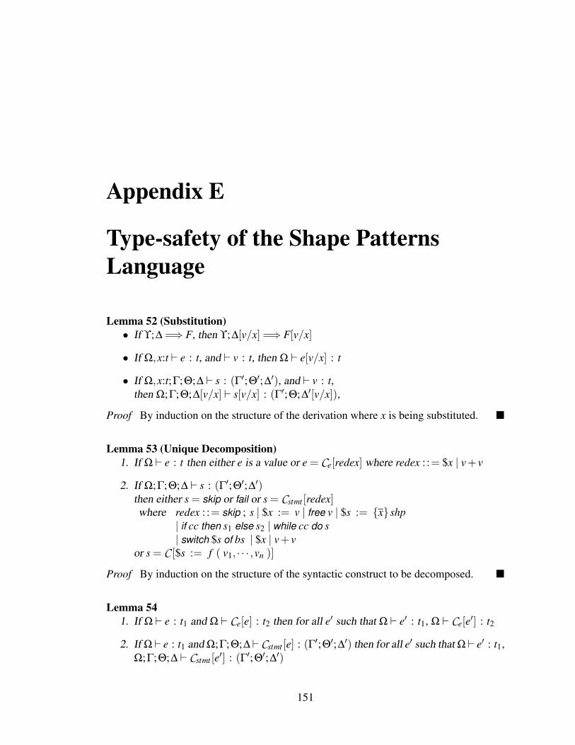
Appendix E
Type-safety of the Shape PatternsLanguage
Lemma 52 (Substitution)• If ϒ;∆ =⇒ F, then ϒ;∆[v/x] =⇒ F[v/x]
• If Ω,x:t ` e : t, and ` v : t, then Ω ` e[v/x] : t
• If Ω,x:t;Γ;Θ;∆ ` s : (Γ′;Θ′;∆′), and ` v : t,then Ω;Γ;Θ;∆[v/x] ` s[v/x] : (Γ′;Θ;∆′[v/x]),
Proof By induction on the structure of the derivation where x is being substituted.
Lemma 53 (Unique Decomposition)1. If Ω ` e : t then either e is a value or e = Ce[redex] where redex : := $x | v+ v
2. If Ω;Γ;Θ;∆ ` s : (Γ′;Θ′;∆′)then either s = skip or fail or s = Cstmt [redex]where redex : := skip ; s | $x := v | free v | $s := xshp
| if cc then s1 else s2 | while cc do s| switch $s of bs | $x | v+ v
or s = C [$s := f ( v1, · · · ,vn )]
Proof By induction on the structure of the syntactic construct to be decomposed.
Lemma 541. If Ω ` e : t1 and Ω ` Ce[e] : t2 then for all e′ such that Ω ` e′ : t1, Ω ` Ce[e′] : t2
2. If Ω` e : t1 and Ω;Γ;Θ;∆` Cstmt [e] : (Γ′;Θ′;∆′) then for all e′ such that Ω` e′ : t1,Ω;Γ;Θ;∆ ` Cstmt [e′] : (Γ′;Θ′;∆′)
151
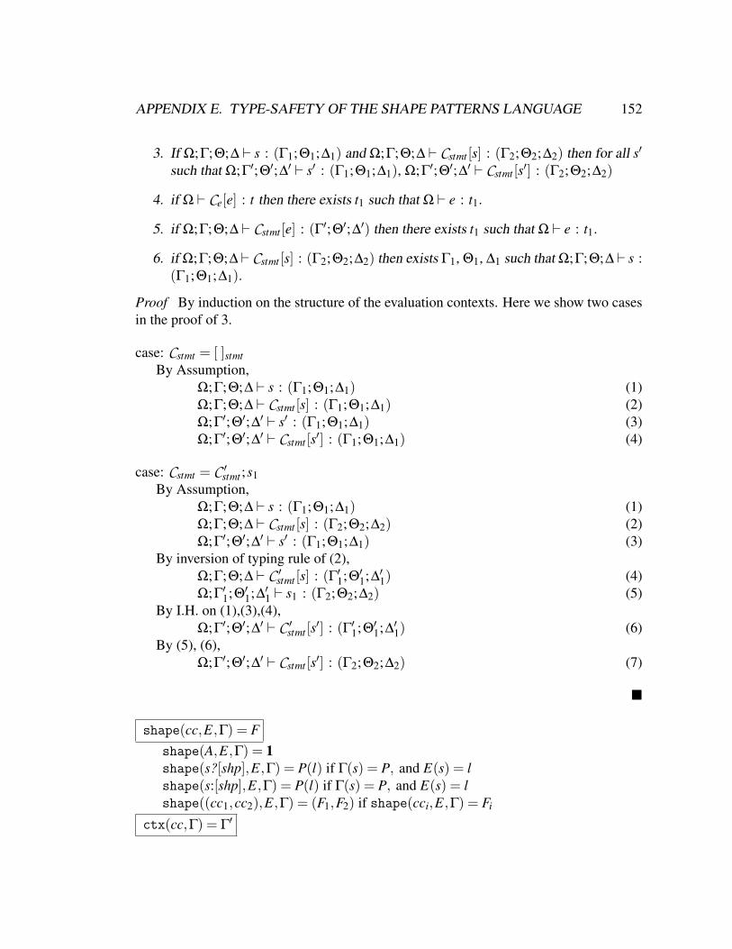
APPENDIX E. TYPE-SAFETY OF THE SHAPE PATTERNS LANGUAGE 152
3. If Ω;Γ;Θ;∆ ` s : (Γ1;Θ1;∆1) and Ω;Γ;Θ;∆ ` Cstmt [s] : (Γ2;Θ2;∆2) then for all s′
such that Ω;Γ′;Θ′;∆′ ` s′ : (Γ1;Θ1;∆1), Ω;Γ′;Θ′;∆′ ` Cstmt [s′] : (Γ2;Θ2;∆2)
4. if Ω ` Ce[e] : t then there exists t1 such that Ω ` e : t1.
5. if Ω;Γ;Θ;∆ ` Cstmt [e] : (Γ′;Θ′;∆′) then there exists t1 such that Ω ` e : t1.
6. if Ω;Γ;Θ;∆ ` Cstmt [s] : (Γ2;Θ2;∆2) then exists Γ1, Θ1, ∆1 such that Ω;Γ;Θ;∆ ` s :(Γ1;Θ1;∆1).
Proof By induction on the structure of the evaluation contexts. Here we show two casesin the proof of 3.
case: Cstmt = [ ]stmtBy Assumption,
Ω;Γ;Θ;∆ ` s : (Γ1;Θ1;∆1) (1)Ω;Γ;Θ;∆ ` Cstmt [s] : (Γ1;Θ1;∆1) (2)Ω;Γ′;Θ′;∆′ ` s′ : (Γ1;Θ1;∆1) (3)Ω;Γ′;Θ′;∆′ ` Cstmt [s′] : (Γ1;Θ1;∆1) (4)
case: Cstmt = C ′stmt ;s1
By Assumption,Ω;Γ;Θ;∆ ` s : (Γ1;Θ1;∆1) (1)Ω;Γ;Θ;∆ ` Cstmt [s] : (Γ2;Θ2;∆2) (2)Ω;Γ′;Θ′;∆′ ` s′ : (Γ1;Θ1;∆1) (3)
By inversion of typing rule of (2),Ω;Γ;Θ;∆ ` C ′
stmt [s] : (Γ′1;Θ′1;∆′1) (4)
Ω;Γ′1;Θ′1;∆′1 ` s1 : (Γ2;Θ2;∆2) (5)
By I.H. on (1),(3),(4),Ω;Γ′;Θ′;∆′ ` C ′
stmt [s′] : (Γ′1;Θ′
1;∆′1) (6)By (5), (6),
Ω;Γ′;Θ′;∆′ ` Cstmt [s′] : (Γ2;Θ2;∆2) (7)
shape(cc,E,Γ) = Fshape(A,E,Γ) = 1shape(s?[shp],E,Γ) = P(l) if Γ(s) = P, and E(s) = lshape(s:[shp],E,Γ) = P(l) if Γ(s) = P, and E(s) = lshape((cc1,cc2),E,Γ) = (F1,F2) if shape(cci,E,Γ) = Fi
ctx(cc,Γ) = Γ′

APPENDIX E. TYPE-SAFETY OF THE SHAPE PATTERNS LANGUAGE 153
ctx(A,E,Γ) = ·ctx(s?[shp],Γ) = s:Γ(s)ctx(s:[shp],Γ) = s:Γ(s)ctx((cc1,cc2),Γ) = (Γ1,Γ2) if ctx(cci,Γ) = Γi
Lemma 55 (Conjunctive Clauses)1. If Ω;Γ ` cc : (Γ′;Θ;∆) and ctx(cc,Γ) = Γcc, then Γ = Γe,Γcc, and Γcc = Γcc1,Γcc2
such that Γ′ = Γe,Γcc1.
2. If Ω;Γ` cc : (Γ′;Θ;∆), and JccKE = (Fcc,σ′) and ctx(cc,Γ) = Γcc, and Γ = Γe,Γcc
such that Γ′ = Γcc1,Γe, and H σ(Fcc), and σ′ ⊆ σ,then H = H1 ]H2 such thatH1 JΓcc1 KE , and H2 σ(∆).
Proof By induction on the structure of cc
1. case:cc = cc1,cc2By assumption,
ctx(cc,Γ) = Γcc (1)Ω;Γ ` cc : (Γ′;Θ;∆) (2)
By definition of ctx(cc),Γcc = Γcc1,Γcc2 (3)such that ctx(cc1) = Γcc1, and ctx(cc2) = Γcc2 (4)
By (2) and the typing rules of cc,Γ = Γ1,Γ2 such that (5)Ω;Γ1 ` cc1 : (Γ′1;Θ′
1;∆1) (6)Ω;Γ2 ` cc2 : (Γ′2;Θ′
2;∆2) (7)Γ′ = Γ′1,Γ
′2, and ∆ = ∆1,∆2 (8)
By I.H. on cc1,Γ1 = Γe1,Γcc1 and Γcc1 = Γcc11,Γcc12 (9)such that Γ′1 = Γe1,Γcc11 (10)
By I.H. on cc2,Γ2 = Γe2,Γcc2 and Γcc2 = Γcc21,Γcc22 (11)such that Γ′2 = Γe2,Γcc21 (12)
By (3), (5),(8),(9),(10),(11),(12),Γ = Γe,Γcc where Γe = Γe1,Γe2such that Γ′ = Γe,Γ
′cc where Γ′cc = Γcc11,Γcc21 (13)
2. case: cc = $s:[root x,FA,F]By assumption,
Ω;Γ ` cc : (Γ′;$s:P;F) where Γ = Γ′,$s:P (1)By (1),
FV(F)∩Ω$ = /0 (2)By definition of JccKE ,

APPENDIX E. TYPE-SAFETY OF THE SHAPE PATTERNS LANGUAGE 154
JccKE = (E(F),E($s)/x) (3)Γcc = $s:P (4)Γcc1 = · (5)Γcc2 = $s:P (6)
By assumption,H ((E($s)/x),σ)(E(FA,F)) (7)
By (7), and the semantics of ⊗ ,H ((E($s)/x),σ)(E(F)) (8)
By (8), and (2),H ((E($s)/x),σ)(F) (9)
Lemma 56If Γ;Π ` cc : Π′, ∀tm ∈ E(Π) is well moded with regard to Hcc, σ′, and E(Π), H′ and H′′
are both subheaps of H, H′ Jctx(Γ,cc)KE , H′′ σ(JccKE), σ′ ⊆ σ, then H′ = H′′.
Proof By induction on the structure of cc, and the Uniqueness of shapes.
Lemma 57 (Safety of CC)If Γ;Π1 ` cc : Π2, shape(cc,E,Γ) = F, H1 F, JccKE = (Fcc,σ), σ⊆ σ′, S⊆ dom(H1),and for all tm such that tm ∈ dom(E(Π1)), tm is well moded with regard to σ, E(Π1) andH1
• either MP(H1 ]H2;S;F;σ′) = (S′,σ′′), and MP will not access location l if l /∈dom(H1), and ∀tm∈ dom(E(Π2)). tm is well moded with regard to σ′′, E(Π2), andH1.
• Or MP(H1]H2;S;F;σ′) = no, and MP will not access location l if l /∈ dom(H1).
Proof By induction on the structure of cc, and using the Safety of MP (Theorem 23).
case: cc = $s?[root x,F]By assumption,
Γ;Π1 ` cc : Π2 (1)By the typing rule of cc and (1),
Ξ;Π1∪x:sf ` F : Π2 where Γ($s) = P,and Ξ = Λ(P) (2)shape(cc,E,Γ) = P(`) where E($s) = ` (3)
By assumption,for all tm such that tm ∈ dom(E(Π1)),tm is well moded with regard to σ,E(Π1) and H1 (4)H1 P(`) (5)

APPENDIX E. TYPE-SAFETY OF THE SHAPE PATTERNS LANGUAGE 155
JccKE = (E(F),`/x) (6)`/x ⊆ σ′ (7)
By Lemma 50 and (2),Ξ;E(Π1∪x:sf) ` E(F) : Π′
2 (8)and Π′
2 < E(Π2) (9)By The safety of MP, and (4), (5), (8),
either MP(H1]H2;S;E(F);σ′) = (S′,σ′′),and MP will not access location ` if ` /∈ dom(H1),and ∀tm ∈ dom(Π′
2), tm is well moded with regard to σ′′,Π′2 and H1. (10)
Or MP(H1]H2;S;F;σ′) = no,and MP will not access location ` if ` /∈ dom(H1). (11)
By (9), (10),∀tm ∈ dom(E(Π2)), tm is well moded with regard to σ′′ and E(Π2) (12)
Theorem 58 (Progress and Preservation)1. if Ω$ ` e : t and ` E : Ω then either e = n or exists e′ such that (E;e) 7−→ e′, and
Ω ` e′ : t
2. if Ω$;Γ;Θ;∆ ` s : (Γ′;Θ′;∆′), ` E : Ω, H JΓKE ⊗∆ then either
• s = skip or fail or
• s = C [x := f ( v1, · · · ,vn )] or
• exists s′, E ′, H′ such that (E;H;s) 7−→ (E ′;H′;s′), and exists Γ′′, Θ′′, ∆′′ suchthat Ω$;Γ′′;Θ′′;∆′′ ` s′ : (Γ′;Θ′;∆′), and ` E ′ : Ω, H′ (JΓK′′E ′)⊗∆′′
3. if ` (E;H;S; fb)OK then either (E;H;S; fb) = (•;H;•;halt)or exists E ′, H′, S′, fb′ such that (E;H;S; fb) 7−→ (E ′;H′;S′; fb′) and ` (E ′;H′;S′; fb′)OK
Proof
1. By induction on the typing judgment Ω$ ` e : t.
2. By examine each case of the unique context decomposition of s.
case: s = C [s′] where s′ = $s:P := x[root (v),F]By assumption,
Ω$;Γ;Θ;∆ ` s : (Γ′;Θ′;∆′) (1)` E : Ω (2)H JΓKE ⊗∆ (3)
By Lemma 54(6) and (1),
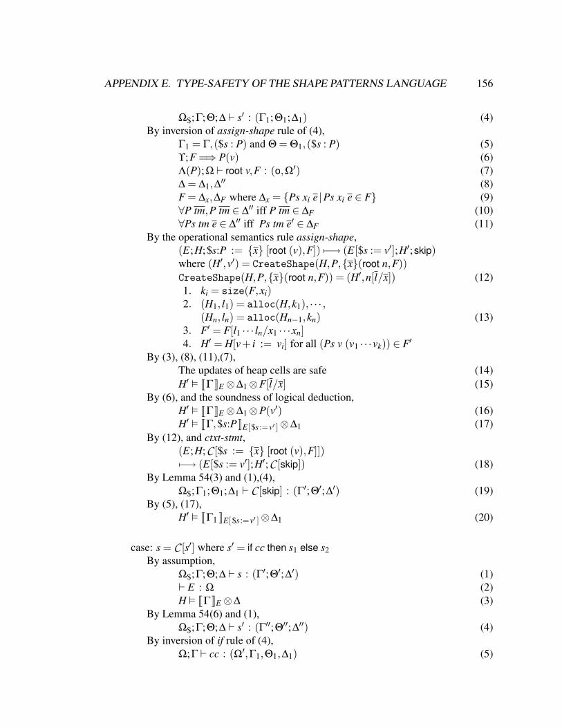
APPENDIX E. TYPE-SAFETY OF THE SHAPE PATTERNS LANGUAGE 156
Ω$;Γ;Θ;∆ ` s′ : (Γ1;Θ1;∆1) (4)By inversion of assign-shape rule of (4),
Γ1 = Γ,($s : P) and Θ = Θ1,($s : P) (5)ϒ;F =⇒ P(v) (6)Λ(P);Ω ` root v,F : (o,Ω′) (7)∆ = ∆1,∆
′′ (8)F = ∆x,∆F where ∆x = Ps xi e |Ps xi e ∈ F (9)∀P tm,P tm ∈ ∆′′ iff P tm ∈ ∆F (10)∀Ps tm e ∈ ∆′′ iff Ps tm e′ ∈ ∆F (11)
By the operational semantics rule assign-shape,(E;H;$s:P := x [root (v),F]) 7−→ (E[$s := v′];H′;skip)where (H′,v′) = CreateShape(H,P,x(root n,F))CreateShape(H,P,x(root n,F)) = (H′,n[l/x]) (12)1. ki = size(F,xi)2. (H1, l1) = alloc(H,k1), · · · ,
(Hn, ln) = alloc(Hn−1,kn)3. F′ = F[l1 · · · ln/x1 · · ·xn]4. H′ = H[v+ i := vi] for all (Ps v (v1 · · ·vk)) ∈ F′
(13)
By (3), (8), (11),(7),The updates of heap cells are safe (14)H′ JΓKE ⊗∆1⊗F[l/x] (15)
By (6), and the soundness of logical deduction,H′ JΓKE ⊗∆1⊗P(v′) (16)H′ JΓ,$s:PKE[$s :=v′ ]⊗∆1 (17)
By (12), and ctxt-stmt,(E;H;C [$s := x [root (v),F]])7−→ (E[$s := v′];H′;C [skip]) (18)
By Lemma 54(3) and (1),(4),Ω$;Γ1;Θ1;∆1 ` C [skip] : (Γ′;Θ′;∆′) (19)
By (5), (17),H′ JΓ1 KE[$s :=v′ ]⊗∆1 (20)
case: s = C [s′] where s′ = if cc then s1 else s2By assumption,
Ω$;Γ;Θ;∆ ` s : (Γ′;Θ′;∆′) (1)` E : Ω (2)H JΓKE ⊗∆ (3)
By Lemma 54(6) and (1),Ω$;Γ;Θ;∆ ` s′ : (Γ′′;Θ′′;∆′′) (4)
By inversion of if rule of (4),Ω;Γ ` cc : (Ω′,Γ1,Θ1,∆1) (5)

APPENDIX E. TYPE-SAFETY OF THE SHAPE PATTERNS LANGUAGE 157
Ω′;Γ1;Θ,Θ1;∆,∆1 ` s1 : (Γ′′;Θ′′;∆′′) (6)Ω;Γ;Θ;∆ ` s2 : (Γ′′;Θ′′;∆′′) (7)Γ;Π ` cc : Π′ where Π = ground(Ω) (8)(E;H; if cc then s1 else s2) 7−→ (E;H;σ(s1))where JccKE = (F,σ′) and MP(H;F; /0;σ′) = (SL;σ) (9)
By Definition of shape(cc,E,Γ),shape(cc,E,Γ) = JΓcc KE where Γcc = ctx(cc,Γ) (10)
By Lemma 55(1),and Γ = Γcc,Γe (11)Γcc = Γcc1,Γcc2, and Γ1 = Γe,Γcc1 (12)
By (3),H = Hcc]He]H∆ (13)such that Hcc JΓcc KE ,He JΓe KE ,H∆ ∆ (14)
By (2), and the definition of ground(Ω),∀tm ∈ dom(E(Π)),tm is well moded with regard to E(Π),σ′,andHcc (15)
By Lemma 57,(8) and (14), (15),MP is memory safe (16)
By The correctness of MP,H′
cc σ(F) (17)By Lemma 56, (8), (14), (15), (17),
H′cc = Hcc (18)
Hcc σ(F) (19)By Lemma 55(2),
Hcc = Hcc1]Hcc2 and Hcc1 JΓcc1 KE (20)and Hcc2 σ(∆1) (21)
By Lemma 52 Substitution and (6),Ω;Γ1;Θ,Θ1;∆,σ(∆1) ` σ(s1) : (Γ′′;Θ′′;∆′′) (22)
By Op semantics rule ctxt-stmt, and (9) ,(E;H;C [if cc then s1 else s2]) 7−→ (E;H;C [σ(s1)]) (23)
By Lemma 54(3) and (1), (22),Ω;Γ1;Θ,Θ1;∆,σ(∆1) ` C [σ(s1)] : (Γ′;Θ′;∆′) (24)
By (13), (14), (19),(20), (21),H JΓ1 KE ⊗∆⊗σ(∆1) (25)
3. By examine the typing rules of ` (E;H;S; fb)OK.
case: the control stack S is empty.By assumption,
` E : Ω H JΓKE ⊗∆ Ω;Γ;Θ;∆ ` fb : τ
` (E .•;H;•; fb)OK (1)
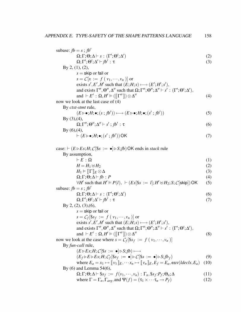
APPENDIX E. TYPE-SAFETY OF THE SHAPE PATTERNS LANGUAGE 158
subase: fb = s ; fb′
Ω;Γ;Θ;∆ ` s : (Γ′;Θ′;∆′) (2)Ω;Γ′;Θ′;∆′ ` fb′ : τ (3)
By 2, (1), (2),s = skip or fail ors = C [x := f ( v1, · · · ,vn )] orexists s′,E ′,H′ such that (E;H;s) 7−→ (E ′;H′;s′),and exists Γ′′,Θ′′,∆′′ such that Ω;Γ′′;Θ′′;∆′′ ` s′ : (Γ′;Θ′;∆′),and ` E ′ : Ω,H′ (JΓ′′ K)⊗∆′′ (4)
now we look at the last case of (4)By ctxt-stmt rule,
(E .•;H;•;(s ; fb′)) 7−→ (E .•;H;•;(s′ ; fb′)) (5)By (3),(4),
Ω;Γ′′;Θ′′;∆′′ ` s′ ; fb′ : τ (6)By (6),(4),
` (E .•;H;•;(s′ ; fb′))OK (7)
case: ` (E .Es;H;C [$s := •].S; fb)OK ends in stack ruleBy assumption,
` E : Ω (1)H = H1]H2 (2)H1 JΓKE ⊗∆ (3)Ω;Γ;Θ;∆ ` fb : P (4)∀H′ such that H′ P(l), ` (Es[$s := l];H′]H2;S;C [skip])OK (5)
subase: fb = s ; fb′
Ω;Γ;Θ;∆ ` s : (Γ′;Θ′;∆′) (6)Ω;Γ′;Θ′;∆′ ` fb′ : τ (7)
By 2, (2), (3),(6),s = skip or fail ors = C f [$s f := f ( v1, · · · ,vn )] orexists s′,E ′,H′ such that (E;H;s) 7−→ (E ′;H′;s′),and exists Γ′′,Θ′′,∆′′ such that Ω;Γ′′;Θ′′;∆′′ ` s′ : (Γ′;Θ′;∆′),and ` E ′ : Ω,H′ (JΓ′′ K)⊗∆′′ (8)
now we look at the case where s = C f [$s f := f ( v1, · · · ,vn )]By fun-call rule,
(E .Es;H;C [$s := •].S; fb) 7−→(E f .E .Es;H;C f [$s f := •].C [$s := •].S; fb f ) (9)where Ea = x1 7→ Jv1 KE , · · ·xn 7→ Jvn KE ,E f = Ea,env(ldecls,Ea) (10)
By (6) and Lemma 54(6),Ω;Γ;Θ;∆ ` $s f := f (v1, · · · ,vn) : Γn,$s f :Pf ;Θn;∆ (11)where Γ = Γn,Γarg,and Ψ( f ) = (τ1×·· ·τn → Pf ) (12)

APPENDIX E. TYPE-SAFETY OF THE SHAPE PATTERNS LANGUAGE 159
By `Φ : Ψ,Ωarg;Γarg f ; ·; · ` ldecls : (Ω f ;Θ f ) (13)and Ω f ;Γarg f ;Θ f ; · ` fb f : Pf , andΓarg f = Γarg[x1, · · ·xn/v1, · · ·vn] (14)
By (10), (12),` E f : Ω f (15)
By (1), (3), (12), (13),H1 = H1a]H1b such that (16)H1a JΓn KE ⊗∆ (17)H1b JΓarg KE (18)
By (10), (14), (18),H1b JΓarg KE f (19)
By (11) and Lemma 54(3),Ω;Γn,$s f :Pf ;Θn;∆ ` (C f ; fb′[skip]) : P (20)
Giving any H f Pf (` f ),By (17),
H f ]H1a JΓn,$s f :Pf KE[$s f :=` f ]⊗∆ (21)By (1),
` E[$s f := ` f ] : Ω (22)By (5), (22), (21),
` (E[$s f := ` f ].Es;H f ]H1a]H2;C [$s := •].S;(C f ; fb′)[skip])OK (23)
By (14),(15),(16),(18) ,(23),` (E f .E .Es;H;C f [$s f := •].C [$s := •].S; fb f )OK (24)
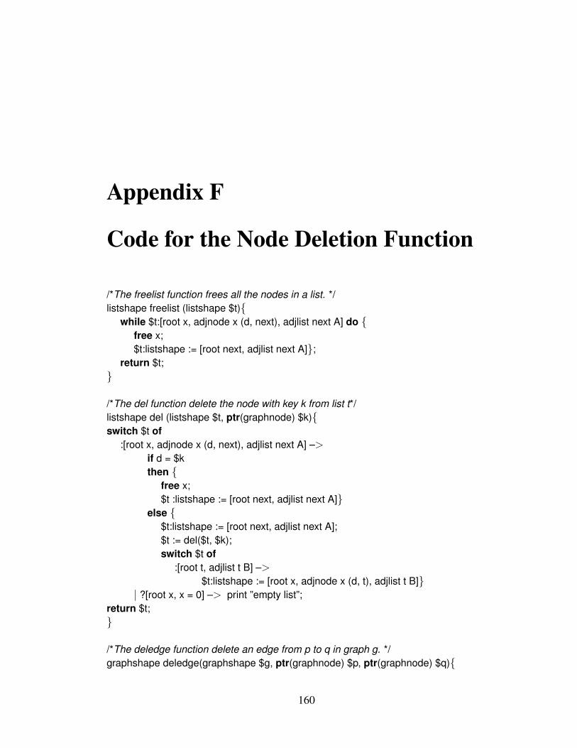
Appendix F
Code for the Node Deletion Function
/*The freelist function frees all the nodes in a list. */listshape freelist (listshape $t)
while $t:[root x, adjnode x (d, next), adjlist next A] do free x;$t:listshape := [root next, adjlist next A];
return $t;
/*The del function delete the node with key k from list t*/listshape del (listshape $t, ptr(graphnode) $k)switch $t of
:[root x, adjnode x (d, next), adjlist next A] –>if d = $kthen
free x;$t :listshape := [root next, adjlist next A]
else $t:listshape := [root next, adjlist next A];$t := del($t, $k);switch $t of
:[root t, adjlist t B] –>$t:listshape := [root x, adjnode x (d, t), adjlist t B]
| ?[root x, x = 0] –> print ”empty list”;return $t;
/*The deledge function delete an edge from p to q in graph g. */graphshape deledge(graphshape $g, ptr(graphnode) $p, ptr(graphnode) $q)
160
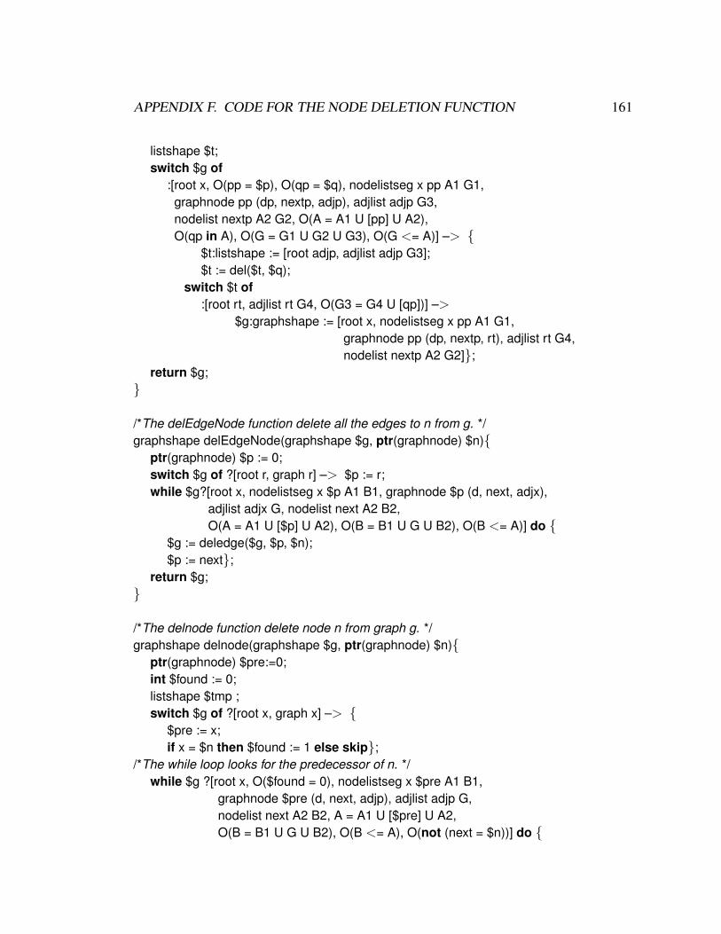
APPENDIX F. CODE FOR THE NODE DELETION FUNCTION 161
listshape $t;switch $g of
:[root x, O(pp = $p), O(qp = $q), nodelistseg x pp A1 G1,graphnode pp (dp, nextp, adjp), adjlist adjp G3,nodelist nextp A2 G2, O(A = A1 U [pp] U A2),O(qp in A), O(G = G1 U G2 U G3), O(G <= A)] –>
$t:listshape := [root adjp, adjlist adjp G3];$t := del($t, $q);
switch $t of:[root rt, adjlist rt G4, O(G3 = G4 U [qp])] –>
$g:graphshape := [root x, nodelistseg x pp A1 G1,graphnode pp (dp, nextp, rt), adjlist rt G4,nodelist nextp A2 G2];
return $g;
/*The delEdgeNode function delete all the edges to n from g. */graphshape delEdgeNode(graphshape $g, ptr(graphnode) $n)
ptr(graphnode) $p := 0;switch $g of ?[root r, graph r] –> $p := r;while $g?[root x, nodelistseg x $p A1 B1, graphnode $p (d, next, adjx),
adjlist adjx G, nodelist next A2 B2,O(A = A1 U [$p] U A2), O(B = B1 U G U B2), O(B <= A)] do
$g := deledge($g, $p, $n);$p := next;
return $g;
/*The delnode function delete node n from graph g. */graphshape delnode(graphshape $g, ptr(graphnode) $n)
ptr(graphnode) $pre:=0;int $found := 0;listshape $tmp ;switch $g of ?[root x, graph x] –>
$pre := x;if x = $n then $found := 1 else skip;
/*The while loop looks for the predecessor of n. */while $g ?[root x, O($found = 0), nodelistseg x $pre A1 B1,
graphnode $pre (d, next, adjp), adjlist adjp G,nodelist next A2 B2, A = A1 U [$pre] U A2,O(B = B1 U G U B2), O(B <= A), O(not (next = $n))] do
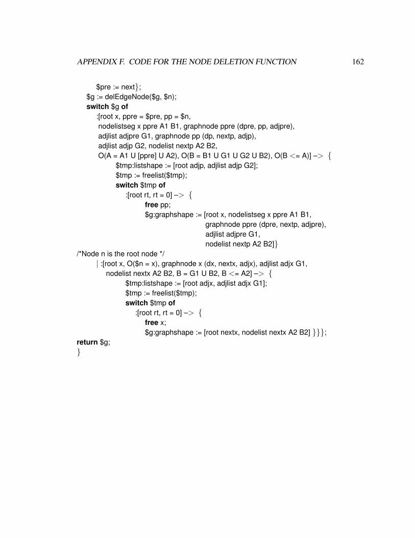
APPENDIX F. CODE FOR THE NODE DELETION FUNCTION 162
$pre := next;$g := delEdgeNode($g, $n);switch $g of
:[root x, ppre = $pre, pp = $n,nodelistseg x ppre A1 B1, graphnode ppre (dpre, pp, adjpre),adjlist adjpre G1, graphnode pp (dp, nextp, adjp),adjlist adjp G2, nodelist nextp A2 B2,O(A = A1 U [ppre] U A2), O(B = B1 U G1 U G2 U B2), O(B <= A)] –>
$tmp:listshape := [root adjp, adjlist adjp G2];$tmp := freelist($tmp);switch $tmp of
:[root rt, rt = 0] –> free pp;$g:graphshape := [root x, nodelistseg x ppre A1 B1,
graphnode ppre (dpre, nextp, adjpre),adjlist adjpre G1,nodelist nextp A2 B2]
/*Node n is the root node */| :[root x, O($n = x), graphnode x (dx, nextx, adjx), adjlist adjx G1,
nodelist nextx A2 B2, B = G1 U B2, B <= A2] –> $tmp:listshape := [root adjx, adjlist adjx G1];$tmp := freelist($tmp);switch $tmp of
:[root rt, rt = 0] –> free x;$g:graphshape := [root nextx, nodelist nextx A2 B2] ;
return $g;

Bibliography
[1] S. Abramsky. Computational interpretations of linear logic. Theoretical ComputerScience, 111:3–57, 1993. 3
[2] P. Aczel. Logical frameworks. In J. Barwise, editor, Handbook of MathematicalLogic, pages 739–782. North-Holland, 1977. 18
[3] A. W. Appel and D. A. McAllester. An indexed model of recursive types forfoundational proof-carrying code. ACM Transactions on Progamming Languagesand Systems, 23(5):657–683, 2001. 20
[4] M. Barnett, K. R. M. Leino, and W. Schulte. The Spec# programming system:an overview. In G. Barthe, L. Burdy, M. Huisman, J.-L. Lanet, and T. Muntean,editors, Post Conference Proceedings of CASSIS: Construction and Analysis of Safe,Secure and Interoperable Smart devices, Marseille, volume 3362 of Lecture Notesin Computer Science, pages 49–69. Springer-Verlag, 2005. 5
[5] C. Barrett and S. Berezin. CVC Lite: A new implementation of the cooperatingvalidity checker. In R. Alur and D. A. Peled, editors, Proceedings of the 16th
International Conference on Computer Aided Verification (CAV ’04), volume 3114of Lecture Notes in Computer Science, pages 515–518. Springer-Verlag, July 2004.Boston, Massachusetts. 15
[6] J. Berdine, C. Calcagno, and P. W. O’Hearn. Smallfoot: Modular automaticassertion checking with separation logic. In International Symposium on FormalMethods for Components and Objects, 2006. 102, 105
[7] D. Beyer, T. A. Henzinger, R. Jhala, and R. Majumdar. Checking memory safetywith blast. In M. Cerioli, editor, FASE, volume 3442 of Lecture Notes in ComputerScience, pages 2–18. Springer, 2005. 104
[8] L. Birkedal, N. Torp-Smith, and J. Reynolds. Local reasoning about a copyinggarbage collector. In ACM Symposium on Principles of Programming Languages,pages 220–231, Venice, Italy, Jan. 2004. 3
163

BIBLIOGRAPHY 164
[9] H.-J. Boehm and M. Weiser. Garbage collection in an uncooperative environment.Software Practice and Experience, 18(9):807–820, Sept. 1988. 106
[10] R. M. Burstall. Some techniques for proving correctness of programs which alterdata structures. In B. Meltzer and D. Michie, editors, Machine Intelligence, pages23–50, Edinburgh, 1972. Edinburgh University Press. 2
[11] W. R. Bush, J. D. Pincus, and D. J. Sielaff. A static analyzer for finding dynamicprogramming errors. Software Practice Experience, 30(7):775–802, 2000. 104
[12] J. Chirimar, C. A. Gunter, and J. G. Riecke. Reference counting as a computationalinterpretation of linear logic. Journal of Functional Programming, 6(2):195–244,Mar. 1996. 3
[13] K. Crary, D. Walker, and G. Morrisett. Typed memory management in a calculusof capabilities. In Twenty-Sixth ACM Symposium on Principles of ProgrammingLanguages, pages 262–275, San Antonio, Jan. 1999. 106
[14] R. Deline and M. Fahndrich. Enforcing high-level protocols in low-level software.In ACM Conference on Programming Language Design and Implementation, pages59–69, Snowbird, Utah, June 2001. ACM Press. 3, 106, 107
[15] D. Detlefs, G. Nelson, and J. B. Saxe. Simplify: a theorem prover for programchecking. 52(3):365–473, 2005. 4, 15
[16] D. L. Detlefs. An overview of the extended static checking system. In The FirstWorkshop on Formal Methods in Software Practice, pages 1–9. ACM(SIGSOFT),Jan. 1996. 36
[17] J. Elgaard, A. Møller, and M. I. Schwartzbach. Compile-time debugging ofC programs working on trees. In G. Smolka, editor, European Symposium onProgramming, volume 1782 of Lecture Notes in Computer Science, pages 119–134.Springer-Verlag, 2000. 104
[18] M. H. V. Emden and R. A. Kowalski. The semantics of predicate logic as aprogramming language. Journal of the ACM, 23(4):733–742, 1976. 18
[19] M. Fahndrich and R. Deline. Adoption and focus: Practical linear types forimperative programming. In ACM Conference on Programming Language Designand Implementation, June 2002. 3, 106
[20] R. B. Findler and M. Felleisen. Contracts for higher-order functions. In ICFP ’02:Proceedings of the seventh ACM SIGPLAN international conference on Functionalprogramming, pages 48–59, New York, NY, USA, 2002. ACM Press. 54

BIBLIOGRAPHY 165
[21] R. W. Floyd. Assigning meaning to programs. In J. T. Schwartz, editor,Mathematical aspects of computer science: Proc. American Mathematics Soc.symposia, volume 19, pages 19–31, Providence RI, 1967. American MathematicalSociety. 2
[22] P. Fradet and D. L. Metayer. Shape types. In Twenty-Fourth ACM Symposium onPrinciples of Programming Languages, 1997. 107
[23] Gerhard Gentzen. Untersuchungen uber das logisches Schließen. MathematischeZeitschrift, 1:176–210, 1935. 21
[24] J.-Y. Girard. Linear logic. Theoretical Computer Science, 50:1–102, 1987. 3
[25] D. Grossman. Safe Programming at the C Level of Abstraction. PhD thesis, CornellUniversity, 2003. 107
[26] D. Grossman, G. Morrisett, T. Jim, M. Hicks, Y. Wang, and J. Cheney. Region-basedMemory Management in Cyclone. In ACM Conference on Programming LanguageDesign and Implementation, Berlin, June 2002. ACM Press. 3, 106
[27] B. Guo, N. Vachharajani, and D. I. August. Shape analysis with inductiverecursion synthesis. In ACM Conference on Programming Language Design andImplementation, pages 256–265, New York, NY, USA, 2007. ACM Press. 105
[28] R. Hastings and B. Joyce. Fast detection of memory leaks and access errors.In Proceedings of the Winter ’92 USENIX conference, pages 125–136. USENIXAssociation, 1992. 104
[29] M. Hauswirth and T. M. Chilimbi. Low-overhead memory leak detection usingadaptive statistical profiling. In ASPLOS, pages 156–164, 2004. 104
[30] J. Henriksen, J. Jensen, M. Jørgensen, N. Klarlund, B. Paige, T. Rauhe, andA. Sandholm. Mona: Monadic second-order logic in practice. In Tools andAlgorithms for the Construction and Analysis of Systems, First InternationalWorkshop, TACAS ’95, LNCS 1019, 1995. 102
[31] M. Hicks, G. Morrisett, D. Grossman, and T. Jim. Experience with safemanual memory-management in cyclone. In International Symposium on MemoryManagement, pages 73–84, Oct. 2004. 107
[32] C. A. R. Hoare. An axiomatic basis for computer programming. Communicationsof the ACM, 12(10):576–580 and 583, October 1969. 2
[33] C. A. R. Hoare. Proof of a program: Find. Communications of the ACM, 14(1):39–45, 1971. 2

BIBLIOGRAPHY 166
[34] R. C. Holt and J. R. Cordy. The Turing programming language. Commun. ACM,31(12):1410–1423, 1988. 54
[35] S. Ishtiaq and P. O’Hearn. BI as an assertion language for mutable data structures.In Twenty-Eighth ACM Symposium on Principles of Programming Languages, Jan.2001. 2, 43, 103, 105
[36] F. Ivanicic, I. Shlyakhter, A. Gupta, and M. K. Ganai. Model checking c programsusing f-soft. In ICCD ’05: Proceedings of the 2005 International Conference onComputer Design, pages 297–308, Washington, DC, USA, 2005. IEEE ComputerSociety. 104
[37] J. L. Jensen, M. E. Jørgensen, N. Klarlund, and M. I. Schwartzbach. Automaticverification of pointer programs using monadic second-order logic. In ACMConference on Programming Language Design and Implementation, pages 226–236, 1997. 104
[38] L. Jia and D. Walker. ILC: A foundation for automated reasoning about pointerprograms. In European Symposium on Programming Languages, Apr. 2006. Toappear. 2
[39] L. Jia and D. Walker. Linear logic, heap-shape patterns and imperative program-ming. Technical Report TR-762-06, Department of Computer Science, Universityof Princeton, 2006. http://www.cs.princeton.edu/ ljia/research/papers/shapes-TR.pdf. 2
[40] T. Jim, J. G. Morrisett, D. Grossman, M. W. Hicks, J. Cheney, and Y. Wang.Cyclone: A safe dialect of C. In General Track: USENIX Annual TechnicalConference, pages 275–288, June 2002. 106
[41] C. C. Josh Berdine and P. O’Hearn. Symbolic execution with separation logic. InAPLAS, pages 52–68, 2005. 105
[42] N. Klarlund and A. Møller. MONA Version 1.4 User Manual. BRICS, Departmentof Computer Science, University of Aarhus, January 2001. 102
[43] N. Klarlund and M. Schwartzbach. Graph types. In Twentieth ACM Symposium onPrinciples of Programming Languages, pages 196–205, Charleston, Jan. 1993. 102
[44] Y. Lafont. The linear abstract machine. Theoretical Computer Science, 59:157–180,1988. 3
[45] T. Lev-Ami and S. Sagiv. TVLA: A system for implementing static analyses.In J. Palsberg, editor, Static Analysis, 7th International Symposium, SAS 2000,Proceedings, volume 1824 of Lecture Notes in Computer Science, pages 280–301.Springer, 2000. 104
BIBLIOGRAPHY 167
[46] P. Lincoln and J. Mitchell. Operational aspects of linear lambda calculus. InSymposium on Logic in Computer Science, pages 235–246. jun 1992. 3
[47] P. Lincoln, J. Mitchell, A. Scedrov, and N. Shankar. Decision problems forpropositional linear logic. Annals of Pure and Applied Logic, 56:239–311, 1992.26, 27, 32
[48] J. Lloyd. Foundations of Logic Programming. Springer-Verlag, 1987. 16
[49] P. Lopez, F. Pfenning, J. Polakow, and K. Watkins. Monadic concurrent linearlogic programming. In The International Conference on Principles and Practice ofDeclarative Programming, 2005. 60
[50] D. C. Luckham. Programming with Specifications: An Introduction to Anna, aLanguage for Specifying ADA Programs. Springer-Verlag, Secaucus, NJ, USA,1990. 54
[51] B. Meyer. Eiffel: programming for reusability and extendibility. SIGPLAN Notices,22(2):85–94, 1987. 54
[52] B. Meyer. Eiffel: the language. Prentice-Hall, Inc., Upper Saddle River, NJ, USA,1992. 54
[53] A. Møller and M. I. Schwartzbach. The pointer assertion logic engine. In ACMConference on Programming Language Design and Implementation, pages 221–231, 2001. 102, 104
[54] G. Morrisett, A. Ahmed, and M. Fluet. L3: A linear language with locations. InInternational Conference on Typed Lambda Calculi and Applications, Apr. 2005. 3,106
[55] G. C. Necula, J. Condit, M. Harren, S. McPeak, and W. Weimer. CCured: type-saferetrofitting of legacy software. ACM Transactions on Progamming Languages andSystems, 27(3):477–526, 2005. 106
[56] G. Nelson and D. C. Oppen. Simplification by cooperating decision procedures.ACM Transactions on Progamming Languages and Systems, 1(2):245–257, 1979.4, 15
[57] P. O’Hearn and D. Pym. The logic of bunched implications. Bulletin of SymbolicLogic, 5(2):215–244, 1999. 103
[58] P. O’Hearn, J. Reynolds, and H. Yang. Local reasoning about programs that alterdata structures. In Computer Science Logic, number 2142 in LNCS, pages 1–19,Paris, 2001. 2, 103, 105
BIBLIOGRAPHY 168
[59] P. W. O’Hearn, H. Yang, and J. C. Reynolds. Separation and information hiding.In POPL ’04: Proceedings of the 31st ACM SIGPLAN-SIGACT symposium onPrinciples of programming languages, pages 268–280, 2004. 73
[60] D. L. Parnas. A technique for software module specification with examples.Communications of the ACM, 15(5):330–336, 1972. 54
[61] F. Perry, L. Jia, and D. Walker. Expressing heap-shape contracts in linear logic.In 5th International Conference on Generative Programming and ComponentEngineering (GPCE), Oct. 2006. 2, 59, 61
[62] F. Pfenning. Structural cut elimination: I. intuitionistic and classical logic.Information and Computation, 157(1-2):84–141, 2000. 24
[63] F. Pfenning. Lecture notes on automated theorem proving. Carnegie MellonUniversity course no. 15-815., 2004. 30
[64] Programming with assertions. http://java.sun.com/j2se/1.4.2/docs/guide/lang/assert.html.54
[65] J. C. Reynolds. Intuitionistic reasoning about shared mutable data structure. InMillennial perspectives in computer science, Palgrove, 2000. 2
[66] J. C. Reynolds. Separation logic: A logic for shared mutable data structures. InProceedings of the 17th Annual IEEE Symposium on Logic in Computer Science,pages 55–74, 2002. 2, 103, 105
[67] M. Sagiv, T. Reps, and R. Wilhelm. Parametric shape analysis via 3-valued logic.In Twenty-Sixth ACM Symposium on Principles of Programming Languages, pages105–118, San Antonio, Jan. 1999. 102, 105
[68] S.C.Kleen. Introduction to Metamathematics. North Holland, 1987. 102
[69] F. Smith, D. Walker, and G. Morrisett. Alias types. In European Symposium onProgramming, pages 366–381, Berlin, Mar. 2000. 3, 106
[70] A. Stump, C. W. Barrett, and D. L. Dill. Cvc: A cooperating validity checker. InCAV ’02: Proceedings of the 14th International Conference on Computer AidedVerification, pages 500–504, London, UK, 2002. Springer-Verlag. 4
[71] D. N. Turner and P. Wadler. Operational interpretations of linear logic. TheoreticalComputer Science, 227:231–248, 1999. Special issue on linear logic. 3
[72] D. N. Turner, P. Wadler, and C. Mossin. Once upon a type. In ACM InternationalConference on Functional Programming and Computer Architecture, San Diego,CA, June 1995. 3

BIBLIOGRAPHY 169
[73] J. D. Ullman. Principles of Database and Knowledge-Base Systems. ComputerScience Press, Rockville, MD, 1988. 16
[74] P. Wadler. Linear types can change the world! In M. Broy and C. Jones, editors,Progarmming Concepts and Methods, Sea of Galilee, Israel, Apr. 1990. NorthHolland. IFIP TC 2 Working Conference. 3
[75] D. Walker. Substructural type systems. In B. C. Pierce, editor, Advanced Topics inTypes and Programming Languages, chapter 1, pages 3–44. The MIT Press, 2004.3
[76] D. Walker, K. Crary, and G. Morrisett. Typed memory management in a calculusof capabilities. ACM Transactions on Programming Languages and Systems,22(4):701–771, May 2000. 3
[77] D. Walker and G. Morrisett. Alias types for recursive data structures. In Workshopon Types in Compilation, Montreal, Sept. 2000. 3, 106
[78] D. Walker and K. Watkins. On linear types and regions. In ACM InternationalConference on Functional Programming, Florence, Sept. 2001. ACM Press. 3
[79] Y. Xie and A. Aiken. Context- and path-sensitive memory leak detection. InESEC/FSE-13: Proceedings of the 10th European software engineering conferenceheld jointly with 13th ACM SIGSOFT international symposium on Foundations ofsoftware engineering, pages 115–125, New York, NY, USA, 2005. ACM Press. 104
[80] D. Zhu and H. Xi. Safe programming with pointers through stateful views. InProceedings of the 7th International Symposium on Practical Aspects of DeclarativeLanguages. Springer-Verlag LNCS vol. 3350, January 2005. 106