linear functions and relationships - connected … functions and relationships ... independent...

Look for these icons that point to enhanced content in Teacher Place

Mathematics BackgroundLinear Functions and Relationships

The goal of this Unit is to develop student understanding of linear functions and equations. A relationship between two variables is a function if each value of one variable (the independent variable) is related to exactly one value of the second variable (the dependent variable). If for each unit change in the independent variable x there is a constant change in the dependent variable y, the relationship is a linear function.

Throughout Moving Straight Ahead, students use tables, graphs, and equations to represent and explore linear functions. The pattern relating two variables in a linear function can be represented with an equation in the form y = mx + b. The coefficient m of the independent variable x indicates the constant rate of change of the dependent variable y and the slope of the straight-line graph of the function. The constant term b is the y-coordinate of the point (0,b) where the graph of the linear function intersects the y-axis. It is called the y-intercept of the graph. Understanding of those key linear function concepts—rate of change, slope, and y-intercept—is developed through exploration of their meaning in specific problem contexts and the patterns in context-free examples.

When a problem involving linear functions requires finding a value of x that corresponds to a specified value of y, the task is to solve a linear equation in the form k = mx + b. Problems in this Unit also develop the understanding and skills students need for success in such equation solving tasks. Students will learn how to inspect tables and graphs of the function y = mx + b to find the required solutions. They will also learn how to use informal and symbolic algebraic reasoning for the same tasks.

The Common Core State Standards for Mathematics reserve introduction of the term function until Grade 8. Thus, throughout this Grade 7 Unit, we talk only about linear relationships between variables. The term linear function will be introduced early in CMP Grade 8 and used throughout that course. Linear relationships will be compared and contrasted with the different patterns of change produced by inverse variation, exponential functions, quadratic functions, and polynomials of higher degree.

Constant Rate of Change and Slope

In Problem 1.2, three students determine their walking rates. Alana walks 1 meter per second, Gilberto walks 2 meters per second, and Leanne walks 2.5 meters per second.

Moving Straight Ahead Unit Planning12

Interactive ContentVideo

CMP14_TG07_U5_UP.indd 12 24/10/13 3:19 PM

UNIT OVERVIEW

GOALS AND STANDARDS

MATHEMATICS BACKGROUND

UNIT INTRODUCTION

UNIT PROJECT

Each walking rate is the constant rate of change relating the variables distance and time. In each case, the dependent variable is the distance d that each person walks, and the independent variable is the time t. The patterns of movement generated by the three walking rates are illustrated by data in the following table.

Time(seconds)

0

1

2

3

4

5

6

7

8

9

10

Distance (meters)

Alana Gilberto

0

1

2

3

4

5

6

7

8

9

10

0

2

4

6

8

10

12

14

16

18

20

Leanne

0

2.5

5

7.5

10

12.5

15

17.5

20

22.5

25

Walking Rates

In the table, the constant rate of change can be observed in the following patterns:

As t increases from 0 to 1 second, d increases by 1 meter for Alana, 2 meters for Gilberto, and 2.5 meters for Leanne. As t increases from 1 to 2 seconds, d increases again by 1 meter for Alana, 2 meters for Gilberto, and 2.5 meters for Leanne.

The patterns continue for each person—as t increases by one unit, d increases by a constant amount.

Each linear relationship can be represented by an equation. In each case, the constant rate of change is the coefficient of t.

d = 1t (Alana)

d = 2t (Gilberto)

d = 2.5t (Leanne)

continued on next page

13Mathematics Background

CMP14_TG07_U5_UP.indd 13 24/10/13 3:19 PM


If we graph pairs of (time, distance) values, each graph is a straight line with slope equal to the corresponding constant rate of change.

Walking Rates

24

18

12

63

21

15

9

00 2 4 6 8 101 3 5 7 9

Dis

tan

ce (

met

ers)

Time (seconds)

Leanne

Gilberto

Alana

The walking rate of 2.5 meters per second is represented by a linear graph with slope steeper than the lines representing the walking rates of 2 meters per second and 1 meter per second.

Students’ understanding of linear situations is strengthened by examining both linear and nonlinear situations throughout the Unit. Most of these occur as tables or graphs like the ones below. Visit Teacher Place at mathdashboard.com/cmp3 to see the complete image gallery.

O–5

–5

5

5

y

x

yx

–3

–2

–1

0

1

2

10

7

4

1

–2

–5

+1

+1

–3

–3

The pattern of change in this relationship is linear. The constant rate of change in thetable is –3 and the y-intercept is 1. The equation for this pattern is y = –3x + 1.

In this Unit, students continue to develop their understanding of proportionality by looking at linear situations that are also proportional relationships. These relationships are represented by the equation y = mx. The constant m is both the constant rate of change for the linear relationship and the constant of proportionality for the proportional relationship. An equation of the form y = mxcan be written in the form

yx = m. Because m is a constant, y is proportional to x.

Students can determine whether a relationship is proportional by looking at a table or a graph for the relationship and observing whether the graph is a straight line through the origin. The constant rate of proportionality, or unit rate, is represented by the constant m in the equation or the point (1, m) on the graph of y = mx. Students can also determine whether a relationship is proportional by testing for equivalent ratios. If the ratios of the coordinates of every point (1, m) are equivalent, then the relationship is proportional.



CMP14_TG07_U5_UP.indd 14 24/10/13 3:19 PM

UNIT OVERVIEW

GOALS AND STANDARDS


UNIT INTRODUCTION

UNIT PROJECT

Rate of Change, Ratio, and Slope of a Line

The constant rate of change for the linear relationship d = 2t is shown in the table and graph below.

Gilberto’s Walking Rate

Time(seconds)

0

1

2

3

4

5

6

7

8

9

+2

+3

0

2

4

6

8

10

12

14

16

18

Distance(meters)

+4

+6

Gilberto’s Walking Rate

16

12

8

4

00 2 4 6 8

d = 2t

Dis

tan

ce (

met

ers)

Time (seconds)

+3

+6

+4

+2

In the table, the constant rate of change is illustrated by reading down both columns. For example, in the table above, the ratio of the change in the dependent variable to the corresponding change in the independent variable is 2 in every case.

In the graph, the constant rate of change is shown by the fact that the ratio of vertical change to horizontal change between any two points on the line is always 2. In this graphic context, the ratio is called the slope of the line. For any two points on the line,

slope = vertical changehorizontal change

In Investigations 1 and 2, linear relationships are characterized by the constant rate of change between the two variables. In Investigation 4, students are introduced to slope as a ratio of the vertical change to the horizontal change between two points on a line. The ratio concept of slope is connected to the constant rate of change between two variables.

Finding the Rate of Change, or Slope, of a Linear Relationship

The slope, or constant rate of change, of a line can be found directly from a verbal description of the problem context, a table of sample values for the independent and dependent variables, an equation for the relationship between the variables, or by finding the ratio of vertical to horizontal changes between two points on the line.



CMP14_TG07_U5_UP.indd 15 24/10/13 3:19 PM


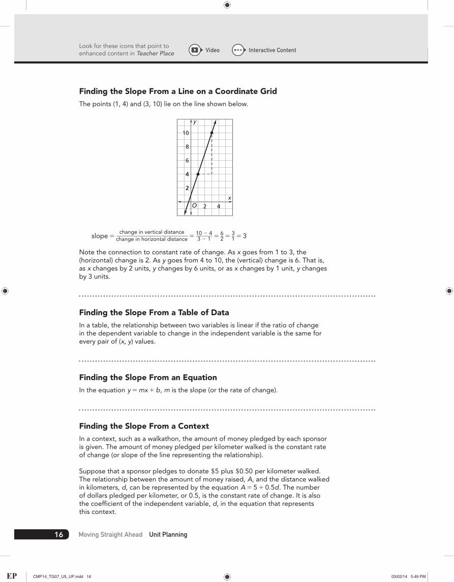
Finding the Slope From a Line on a Coordinate GridThe points (1, 4) and (3, 10) lie on the line shown below.

O 2 4

2

x

2

4

6

4

8

10

y

slope = change in vertical distancechange in horizontal distance = 10 - 4

3 - 1 = 62 = 3

1 = 3

Note the connection to constant rate of change. As x goes from 1 to 3, the (horizontal) change is 2. As y goes from 4 to 10, the (vertical) change is 6. That is, as x changes by 2 units, y changes by 6 units, or as x changes by 1 unit, y changes by 3 units.

Finding the Slope From a Table of DataIn a table, the relationship between two variables is linear if the ratio of change in the dependent variable to change in the independent variable is the same for every pair of (x, y) values.

Finding the Slope From an EquationIn the equation y = mx + b, m is the slope (or the rate of change).

Finding the Slope From a ContextIn a context, such as a walkathon, the amount of money pledged by each sponsor is given. The amount of money pledged per kilometer walked is the constant rate of change (or slope of the line representing the relationship).

Suppose that a sponsor pledges to donate +5 plus +0.50 per kilometer walked. The relationship between the amount of money raised, A, and the distance walked in kilometers, d, can be represented by the equation A = 5 + 0.5d. The number of dollars pledged per kilometer, or 0.5, is the constant rate of change. It is also the coefficient of the independent variable, d, in the equation that represents this context.



CMP14_TG07_U5_UP.indd 16 03/02/14 5:49 PM

UNIT OVERVIEW

GOALS AND STANDARDS


UNIT INTRODUCTION

UNIT PROJECT

Finding the y-Intercept and Equation for a Linear Relationship

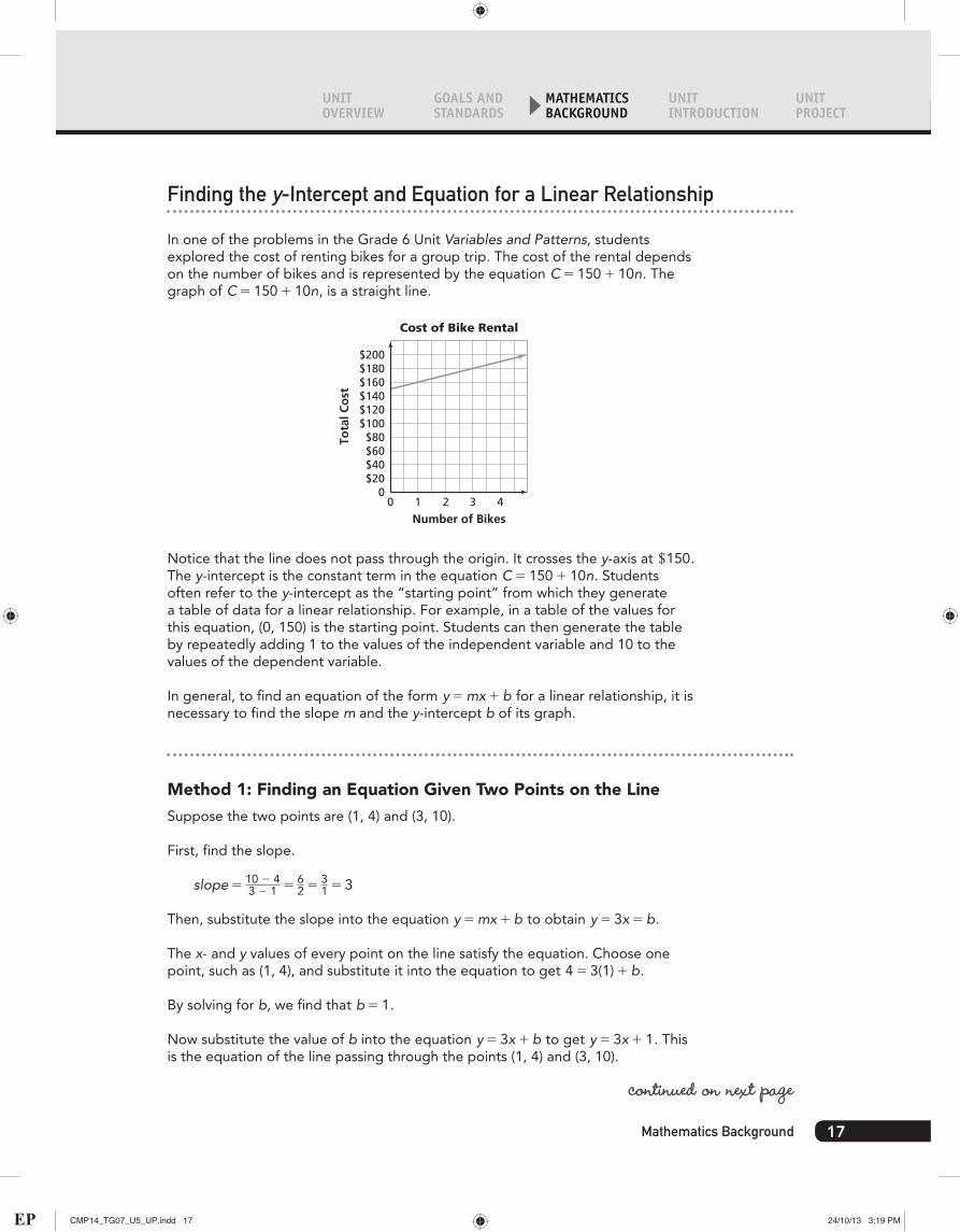
In one of the problems in the Grade 6 Unit Variables and Patterns, students explored the cost of renting bikes for a group trip. The cost of the rental depends on the number of bikes and is represented by the equation C = 150 + 10n. The graph of C = 150 + 10n, is a straight line.

Cost of Bike Rental

$20$40$60$80

$100$120$140$160$180$200

00 1 2 3 4

Tota

l Co

st

Number of Bikes

Notice that the line does not pass through the origin. It crosses the y-axis at +150. The y-intercept is the constant term in the equation C = 150 + 10n. Students often refer to the y-intercept as the “starting point” from which they generate a table of data for a linear relationship. For example, in a table of the values for this equation, (0, 150) is the starting point. Students can then generate the table by repeatedly adding 1 to the values of the independent variable and 10 to the values of the dependent variable.

In general, to find an equation of the form y = mx + b for a linear relationship, it is necessary to find the slope m and the y-intercept b of its graph.

Method 1: Finding an Equation Given Two Points on the LineSuppose the two points are (1, 4) and (3, 10).

First, find the slope.

slope = 10 - 43 - 1 = 6

2 = 31 = 3

Then, substitute the slope into the equation y = mx + b to obtain y = 3x = b.

The x- and y values of every point on the line satisfy the equation. Choose one point, such as (1, 4), and substitute it into the equation to get 4 = 3(1) + b.

By solving for b, we find that b = 1.

Now substitute the value of b into the equation y = 3x + b to get y = 3x + 1. This is the equation of the line passing through the points (1, 4) and (3, 10).



CMP14_TG07_U5_UP.indd 17 24/10/13 3:19 PM


Method 2: Finding an Equation From a Table of DataConsider the following table.

yx

3

4

5

6

7

7

10

13

16

19

First, note that the data in the table represent a linear relationship because as x increases by 1 unit, y increases by 3 units. The constant rate of change, or slope, is 3.

Then, to find the y-intercept, you can follow the steps used in Method 1. Or, you can simply use the rate of change to work backwards in the table until x = 0. That is, as x decreases by 1 unit, y decreases by 3 units. This is repeated until x = 0.

yx

0

1

2

3

4

5

−2

1

4

7

10

13

The y-intercept is -2. So the equation that represents the data in the table is y = 3x - 2.

Method 3: Finding an Equation From a GraphFirst, find the y-intercept directly or by extending the line to intersect the y-axis. In the example pictured below, the y-intercept is 1, because the line crosses the y-axis at (0, 1).

O 2 4

2

x

2

4

6

4

8

10

y



CMP14_TG07_U5_UP.indd 18 24/10/13 3:19 PM

UNIT OVERVIEW

GOALS AND STANDARDS


UNIT INTRODUCTION

UNIT PROJECT

Then, find the slope by picking any two points on the line and applying the definition of slope. For example, in the graph above, the points (3, 10) and (1, 4) indicate a slope of 3.

Thus, the equation for the line is y = 3x + 1.

Linear Equations

Throughout this Unit, students use various representations (graphs, tables, equations, and verbal descriptions) to explore situations that involve linear relationships. They are asked to find information about one of the variables given information about the other. They can find this information from tables, from graphs, or by reasoning numerically. They can also apply properties of equality to solve a linear equation in one unknown symbolically.

Consider the equation y = 5x - 10. Suppose that the value of x is known to be 3. Then, to find the value of y, you can solve the equation y = 5(3) - 10. In this case, it is just a matter of applying arithmetic calculations to the expression 5(3) - 10. This is more commonly called evaluating the expression 5x - 10 when x = 3. Suppose that the value of y is known to be 15. You can find the value of x by solving the equation 15 = 5x - 10, but it is not as straightforward.

Solving linear equations in one unknown involves finding information about one of the variables in a linear relationship. When students are asked to solve the equation 26 = 9 - 2x, they can associate this equation in one unknown with the equation y = 9 - 2x and look for values of x that correspond to y = 26.

Solving a Linear Equation

The key to solving equations symbolically is understanding equality. Many students think of the equal sign as a signal to “do something.” For example, in elementary grades students encounter questions like these:

6 + 15 = ■ 6 # 13 + 15 = ■

As a consequence, they often come to think of an equation as a sequence of calculations on a set of numbers to get an answer. This can be a source of misconceptions. Instead, an equation is a statement that two quantities are equal. In this Unit, students develop an understanding of equality that can be thought of as a “balance.” They learn how to write given equations in progressively simpler equivalent forms, which maintain the equality, or the balance, between two quantities.



CMP14_TG07_U5_UP.indd 19 24/10/13 3:19 PM


In Investigations 1 and 2, students are frequently asked to find the value of one variable in a linear relationship when given information about the other variable. For instance, in the equation A = 5 + 0.50d, where A is the amount of money raised and d is the distance walked in kilometers, we might want to know how far a student would have to walk in order to raise +10. Answering that question requires solving a linear equation with one variable or “one unknown.” Students can find the value of the variable by using various methods.

• Solve the equation using symbolic methods.

• Interpret the information from a table or a graph.

• Reason about the situation in verbal form—“There is a fixed pledge of +5 and then a donation of +0.50 per kilometer. By subtracting 5 from 10, we get +5 for the total amount donated based on the distance walked. If we divide this by 0.50, we get 10 kilometers.”

Investigation 3 develops symbolic methods for solving equations. To solve an equation symbolically, we write a series of equivalent equations until we have one from which it is easy to read the value of the variable.

Equivalent equations have the same solutions. Equality or equivalence can be maintained by adding, subtracting, multiplying, or dividing the same quantity on both sides of the equation. For multiplication and division, the quantity must be nonzero. These properties are called the properties of equality.

Students explore the properties of equality informally by examining metaphorical equations that involve +1 gold coins and mystery pouches of coins. We assume that all pouches in an equation have the same number of coins and that both sides of the equality sign have the same number of coins. Visit Teacher Place at mathdashboard.com/cmp3 to see the complete video.

This provides a transition to the more abstract method of solving linear equations in one unknown. Students first find the number of coins using the pictures. Then, they translate each picture into a symbolic statement. For example, if x represents the number of coins in a pouch, then the preceding pictorial statement can be represented as 5 = 2x + 1. Next, students apply the properties of equality to isolate the variable—that is, they solve the equation for x.



CMP14_TG07_U5_UP.indd 20 24/10/13 3:19 PM

UNIT OVERVIEW

GOALS AND STANDARDS


UNIT INTRODUCTION

UNIT PROJECT

In this Unit, we solve equations with complexity like these examples:

6 - 3x = 10

5 + 17x = 12x - 9

2(x + 3) = 10

An understanding of integers was developed in Accentuate the Negative. An understanding of the Distributive Property was developed in Prime Time, Accentuate the Negative, and Variables and Patterns. Review of integers and the Distributive Property is also provided in the Connections section of the ACE Exercises.

Solving a System of Two Linear Equations

Students informally solve systems of linear equations throughout the Unit. They use graphs and tables to find the point of intersection of two lines. For example, in Problems 2.1 and 2.2, students compare walking rates of two brothers who are racing. In order to find the length of a race that will allow the younger brother to win in a close race, students are asked to determine when the brothers’ distances from the starting point are equal.

The equations below represent the relationships between time and each brother’s distance from the starting point. In eqch equation, d represents the distance, in meters, that each brother is from the starting point at time t.

dEmile = 2.5t

dHenri = 45 + t

To find the time at which Emile will catch up with Henri and their distances will be equal, students can use a table to find when the values of (t, d) are the same. Or, they can graph the equations and find the point of intersection of the two lines.

Later, students will learn how to solve the preceding system of equations symbolically. To find when Emile’s distance equals Henri’s distance, they would write 2.5t = 45 + t and solve for t. In Investigation 3, students learn that situations like this one can be represented by a system of linear equations. Thus, without calling attention to it, students have solved a linear system.

It is important that students understand what a solution to an equation means, whether they are dealing with a symbolic solution or a graphical solution. It is also important that they connect these two representations of a solution. In the preceding example, t = 30 is a solution of 2.5t = 45 + t. It means that if Emile and Henri walk in their race for 30 seconds, they will be the same distance from the starting point. Graphically, the lines y = 2.5x and y = 45 + x intersect at (30, 75). This solution means that when the brothers each walk for 30 seconds, they are both 75 meters from the starting point. If the race were to end at this point, they would tie.


CMP14_TG07_U5_UP.indd 21 24/10/13 3:19 PM


Inequalities

Investigations 1 and 2, ideas about inequality are informally explored by asking questions like this: “If x = 4, does Gilberto raise more or less money than Alana?” Students can answer this question by substituting 4 for x in y = 2x and y = 5 + 0.5x and then comparing the y-values.

In Investigation 3, solving linear inequalities using graphs evolves naturally from contexts such as Fabian’s Bakery in Problem 3.5. In this Problem, the bakery’s expenses for making and selling n cakes can be represented by the equation E = 825 + 3.25n. The bakery’s income for selling n cakes is represented by the equation I = 8.20n.

In Question C, students apply their knowledge of how to solve a linear equation to find the break-even point, or the value of n, for which E = I or 825 + 3.25n = 8.20n.

In Question E, students are asked to find the number of cakes for which the bakery’s expenses are less than +2,400 and the number of cakes for which the bakery’s income is greater than +2,400. This requires students to use their knowledge of inequalities from Accentuate the Negative to find the solution set to the inequality statements 825 + 3.25n 6 2,400 and 8.20n 7 2,400. They can graph the associated equations and then find the values of n that satisfy the inequalities. Visit Teacher Place at mathdashboard.com/cmp3 to see the complete video.

Equivalent Expressions

Two arithmetic expressions are equivalent if they have the same numerical value. For example, 7 - 8 is equivalent to 7 + (-8). Two algebraic expressions are equivalent if they have the same numerical value regardless of the values of the variables involved. For example, a - b is equivalent to a + (-b).



CMP14_TG07_U5_UP.indd 22 03/02/14 5:51 PM

UNIT OVERVIEW

GOALS AND STANDARDS


UNIT INTRODUCTION

UNIT PROJECT

Equivalent expressions were first introduced in Grade 6 using the Distributive Property—first as equivalent numerical expressions in Prime Time and then as equivalent algebraic expressions in Variables and Patterns. For example, the product of the two factors 3 and (5 + 8) can be written as the sum of the two terms 3(5) and 3(8). That is, 3(5 + 8) = 3(5) + 3(8). Similarly, 3(x + 2) = 3(x) + 3(2). Area models were used to develop understanding of the Distributive Property.

5

3

8 x

3

2

The Distributive Property also provides a way to add “like terms.” For example, 3x and 5x are like terms. They have the same variable(s); 3x + 5x is equivalent to (3 + 5)x or 8x.

x

3

5

In this Unit, equivalent expressions arise in Problems 3.2 and 3.3 as students solve equations involving pouches filled with gold coins. (See the examples on the Mathematics Background page Solving a Linear Equation.) Visit Teacher Place at mathdashboard.com/cmp3 to see the complete video.



CMP14_TG07_U5_UP.indd 23 03/02/14 5:52 PM


Equivalent expressions also surface in Problem 3.5. In Question A, students are given equations for the income I and the expenses E of a bakery. They are asked to find an equation for profit. Some students may write 8.2n - (825 + 3.25n) to represent the profit. Others may write 4.95n - 825. The properties of numbers can be used to show that the two expressions are equivalent. See the discussion on the Mathematics Background page Linear Inequalities for further information about this Problem.

In Problem 4.4, students find an equation for perimeter P of Figure n made from square tiles.

Figure 1 Figure 2 Figure 3

Students might find several equivalent expressions for the perimeter, such as 4n + 2, 3n + (n - 1) + 3, or even 2(n + 1) + 2n. Properties of numbers can show that these expressions are equivalent.

One of the more important aspects of equivalent expressions is that they reveal different pieces of information about the context. Students who come up with the expression 4n + 2 could be thinking of each figure as consisting of two squares, one that is n * n and another that is 1 * 1. Those who arrive at the expression 2(n + 1) + 2n could be thinking about the perimeter of a rectangle with dimensions n + 1 and n. The missing squares do not affect the perimeter. The expression 3n + (n - 1) + 3 suggests looking at three sides of the figure of length n and then the remaining lengths are (n - 1) and 3 (this represents the perimeter of the unit square at the right of each figure.)

n

4n + 2

n

1

1

n n

n

3n + (n – 1) + 3

n

1

1n

n – 1

n + 12(n + 1) + 2n

n

n 1 n



CMP14_TG07_U5_UP.indd 24 24/10/13 3:19 PM

linear functions and relationships - connected … functions and relationships ... independent...

Documents