linear estimation and causal wiener-kolmogorov filtering - spinlab

ECE531 Lecture 12: Linear Estimation and Causal W-K Filtering

ECE531 Lecture 12: Linear Estimation and Causal

Wiener-Kolmogorov Filtering

D. Richard Brown III

Worcester Polytechnic Institute

16-Apr-2009

Worcester Polytechnic Institute D. Richard Brown III 16-Apr-2009 1 / 51


Introduction

◮ General (static or dynamic) Bayesian MMSE estimation problem:Determine unknown state/parameter X[ℓ] from observationsY [a], Y [a + 1] . . . , Y [b] for some b ≥ a.

◮ Prediction: ℓ > b.◮ Estimation: ℓ = b.◮ Smoothing: ℓ < b.

◮ General solution is just the conditional mean:

Xmmse[ℓ] = E {X[ℓ] |Y [a], . . . , Y [b]}

◮ This problem is difficult to compute in general. Two approaches togetting useful results:

◮ Restrict the model, e.g. linear and white Gaussian. This led to aclosed-form batch solution and the discrete-time Kalman-Bucy filter.

◮ Restrict the class of estimators, e.g. unbiased or linear estimators.

◮ Linear estimators are particularly interesting since they arecomputationally convenient and require only partial statistics.



Jointly Gaussian MMSE Estimation

Suppose that X[ℓ], Y [a], . . . , Y [b] are jointly Gaussian random vectors. Weknow that

Xmmse[ℓ] = E {X [ℓ] |Y [a], . . . , Y [b]}

= E{X [ℓ] |Y b

a

}

= E{X [ℓ]}+ cov{X [ℓ], Y b

a }[cov{Y b

a , Y b

a }]−1 (

Y b

a − E{Y b

a })

= H⊤[a, b, ℓ]Y b

a + c[a, b, ℓ]

where H[a, b, ℓ] is a matrix with dimensions (b − a + 1)k × m and c[a, b, ℓ]is a vector of dimension m × 1.

Note that the MMSE estimate in this case is simply a linear (affine)combination of the “super-vector” of observations Y b

a plus some constant.

When X[ℓ], Y [a], . . . , Y [b] are jointly Gaussian random vectors, the MMSEestimator is a linear estimator. In this particular case, the restriction tolinear estimators results in no loss of optimality.



Basics of Linear Estimators

A linear estimator for the state/parameter X[ℓ] given the observationsY [a], Y [a + 1] . . . , Y [b] for some b ≥ a is simply a collection of linearweights applied to the observations with possibly a constant offset notdepending on the observations. When b − a is finite, we can write

X[ℓ] = H⊤[a, b, ℓ]Y ba + c[a, b, ℓ] ∈ R

m

Remarks:

◮ This expression is for general vector-valued parameters/states.

◮ Note that the kth element of the estimate is affected only by the kthrow of H⊤[a, b, ℓ] and the kth element of c[a, b, ℓ]:

Xk[ℓ] = h⊤k [a, b, l]Y b

a + ck[a, b, ℓ] ∈ R

◮ Since we can pick the coefficients in each row of H⊤[a, b, ℓ] andc[a, b, ℓ] without affecting the other estimates, we can focus herewithout any loss of generality on the case when X [ℓ] is a scalar.



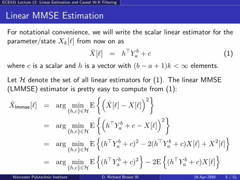
Linear MMSE Estimation

For notational convenience, we will write the scalar linear estimator for theparameter/state Xk[ℓ] from now on as

X [ℓ] = h⊤Y ba + c (1)

where c is a scalar and h is a vector with (b − a + 1)k < ∞ elements.

Let H denote the set of all linear estimators for (1). The linear MMSE(LMMSE) estimator is pretty easy to compute from (1):

Xlmmse[ℓ] = arg min{h,c}∈H

E

{(

X[ℓ] − X[ℓ])2}

= arg min{h,c}∈H

E

{(

h⊤Y ba + c − X[ℓ]

)2}

= arg min{h,c}∈H

E{

(h⊤Y ba + c)2 − 2(h⊤Y b

a + c)X[ℓ] + X2[ℓ]}

= arg min{h,c}∈H

E{

(h⊤Y ba + c)2

}

− 2E{

(h⊤Y ba + c)X[ℓ]

}



Linear MMSE Estimation (continued)

Picking up where we left off...

Xlmmse[ℓ] = arg min{h,c}∈H

E{

(h⊤Y ba + c)2

}

− 2E{

(h⊤Y ba + c)X[ℓ]

}

= arg min{h,c}∈H

h⊤E{

Y ba (Y b

a )⊤}

h + 2ch⊤E{

Y ba

}

+ c2

−2[

h⊤E{

Y ba X[ℓ]

}

+ cE {X[ℓ]}]

What should we do now? Let’s take the gradient with respect to [h, c]⊤

and set it equal to zero...

[2E{Y b

a (Y ba )⊤

}h + 2cE

{Y b

a

}− 2E

{Y b

a X[ℓ]}

2E{(Y b

a )⊤}

h + 2c − 2E {X[ℓ]}

]

=

[00

]

The second equation implies that c = E{X[ℓ]} − E{(Y b

a )⊤}

h. Plug thisinto first equation and solve for h...




First equation:

2E{

Y ba (Y b

a )⊤}

h + 2cE{

Y ba

}

− 2E{

Y ba X[ℓ]

}

= 0

Plug in c = E{X[ℓ]} − E{(Y b

a )⊤}

h...

E{Y b

a(Y b

a)⊤}

h + E{Y b

a

}E {X [ℓ]} − E

{Y b

a

}E{(Y b

a)⊤}

h − E{Y b

aX [ℓ]

}= 0

Collecting terms and recognizing that

cov(Y, Y ) = E{Y Y ⊤} − E{Y }E{Y ⊤}

cov(Y,X) = E{Y X} − E{Y }E{X} (when X is a scalar)

we can write

hlmmse =[

cov(Y ba , Y b

a )]−1

cov(Y ba ,X[ℓ])

Sanity check: What are the dimensions of hlmmse?Worcester Polytechnic Institute D. Richard Brown III 16-Apr-2009 7 / 51



Putting it all together, we have

Xlmmse[ℓ] = h⊤

lmmseYb

a+ c

= h⊤

lmmseYb

a + E{X [ℓ]} − h⊤

lmmseE{Y b

a

}

= E{X [ℓ]}+ h⊤

lmmse

(Y b

a − E{Y b

a

})

= E{X [ℓ]}+ cov(X [ℓ], Y b

a )[cov(Y b

a , Y b

a )]−1 (

Y b

a − E{Y b

a

})

This should look familiar.

◮ It should be clear that Xlmmse[ℓ] = Xmmse[ℓ] when X [ℓ], Y [a], . . . , Y [b] arejointly Gaussian.

◮ Computation of Xlmmse[ℓ] only requies knowledge of the observation/statemeans and covariances (second order statistics). This is much moreappealing than requiring full knowledge of the joint distributions.

◮ Since the role of c is only to compensate for any non-zero mean of Xlmmse[ℓ]and any non-zero mean of Y b

a , we can assume without loss of generality thatE{X [ℓ]} ≡ 0 and E{Y b

a } ≡ 0 (and hence c = 0) from now on.



Extension to Vector LMMSE State Estimator

Our result for the scalar LMMSE state estimator (X[ℓ] ∈ R) :

hlmmse =[

cov(Y ba , Y b

a )]−1

cov(Y ba ,X[ℓ])

︸︷︷︸

vector

The vector LMMSE state estimator (X[ℓ] ∈ Rm) can be written as

Hlmmse :=[h0

lmmse, . . . hm−1lmmse

]

and we can write

Hlmmse =[

cov(Y ba , Y b

a )]−1 [

cov(Y ba ,X0[ℓ]), . . . , cov(Y b

a ,Xm−1[ℓ])]

=[

cov(Y ba , Y b

a )]−1

cov(Y ba ,X[ℓ])

︸︷︷︸

matrix

where X[ℓ] = [X0[ℓ], . . . ,Xm−1[ℓ]]⊤.



Remarks

◮ Note that the only assumptions/restrictions that we have made so farin the development of the LMMSE estimator are

1. We only consider linear (affine) estimators.2. We only consider the MSE cost assignment.3. The number of observations b − a + 1 is finite.4. The matrix cov(Y b

a, Y b

a) is invertible.

◮ Other than some mild regularity conditions (finite expectations for theobservations and the state), we have made no assumptions about thestatistical nature of the observations or the unknown state/parameter.

◮ Hence, this result is quite general.

◮ Practicality of direct implementation is limited somewhat by therequirement to compute a matrix inverse. The Kalman filter (and itsextensions) alleviates this problem in some cases.

◮ What can we say about the case when cov(Y ba , Y b

a ) is not invertible?



Covariance Matrix and MSE of Linear Estimation

In the general vector parameter case, let

CXX := cov(X[ℓ],X[ℓ])

CXY := cov(X[ℓ], Y ba ) = C⊤

Y X

CY Y := cov(Y ba , Y b

a )

We can write the covariance matrix of the LMMSE estimator as

Clmmse := E{

(X[ℓ] − X [ℓ])(X[ℓ] − X[ℓ])⊤}

= E{[

X[ℓ] − E{X[ℓ]} − CXY C−1Y Y

(

Y ba − E

{

Y ba

})] [same

]⊤}

= CXX − 2CXY C−1Y Y CY X + CXY C−1

Y Y CY Y C−1Y Y CY X

= CXX − CXY C−1Y Y CY X

The variance of each individual parameter estimate is on the diagonal ofthis covariance matrix. What can we say about the overall MSE?



Two-Coefficient Scalar LMMSE Estimation

Consider a two-coefficient time-invariant linear estimator h = [h0, h1]⊤ for

the scalar state X[ℓ] based on the scalar observations Y [ℓ − 1] and Y [ℓ].Also assume that X[ℓ] and Y [ℓ] are wide-sense stationary (andcross-stationary) and that E{X[ℓ]} = E{Y [ℓ]} = 0 such that c = 0.

The MSE of the linear estimator h can be written as

MSE := E{

(X [ℓ] − X[ℓ])2}

= h⊤E{

Y ba (Y b

a )⊤}

h − 2h⊤E{

Y ba X[ℓ]

}

+ E{X2[ℓ]

}

= h⊤CY Y h − 2h⊤CY X + σ2X

An LMMSE estimator must satisfy CY Y hlmmse = CY X . When CY Y isinvertible, the unique LMMSE estimator is simply

hlmmse = C−1Y Y CY X .

Since we only have two coefficients in our linear estimator, we can plot theMSE as a function of these coefficients to get some intuition...



Unique LMMSE Solution (CY Y is invertible)

h0

h1

−1 −0.8 −0.6 −0.4 −0.2 0 0.2 0.4 0.6 0.8 1−1

−0.8

−0.6

−0.4

−0.2

0

0.2

0.4

0.6

0.8

1



Non-Unique LMMSE Solution (CY Y is not invertible)

h0

h1

−1 −0.8 −0.6 −0.4 −0.2 0 0.2 0.4 0.6 0.8 1−1

−0.8

−0.6

−0.4

−0.2

0

0.2

0.4

0.6

0.8

1

Hint: Use Matlab’s pinv function to find the minimum norm solution.Worcester Polytechnic Institute D. Richard Brown III 16-Apr-2009 14 / 51


Infinite Number of Observations

The case we have yet to consider is when b− a is not finite. For notationalsimplicity, we will focus here on scalar states X[ℓ] ∈ R and scalarobservations Y [ℓ] ∈ R. The main ideas developed here can be extended tothe vector cases without too much difficulty.

In the cases when a = −∞, or b = ∞, or both a = −∞ and b = ∞, wecan no longer use our matrix-vector notation. Instead, a linear estimatorfor X[ℓ] must be written as the sum

X[ℓ] =

b∑

k=a

h[ℓ, k]Y [k] + c[ℓ] ∈ R

In particular, we are going to have be careful about the exchange ofexpectations and summations since the summations are no longer finite.



Exchange of Summation and Expectation

Theorem (Poor V.C.1)

Given E{Y 2[k]} < ∞ for all k, h[ℓ, k] ∈ R for all ℓ, k, and

X[ℓ] =

b∑

k=a

h[ℓ, k]Y [k] + c[ℓ]

for b ≥ a, then E{(X[ℓ])2} < ∞. Moreover, if Z is any random variable

satisfying E{Z2} < ∞ then

E{ZX[ℓ]} =b∑

k=a

h[ℓ, k]E{ZY [k]} + c[ℓ]E{Z}.

This theorem is obviously true when a and b are finite. The second result is a

little bit tricky (but important) to show for the cases when a = −∞, or b = ∞,

or both a = −∞ and b = ∞.



Convergence In Mean Square for Infinite Sums

Although not explicit in the theorem, the proof for case when we have aninfinite number of observations is going to require that the infinite sums ofrandom variables in the estimates converge in mean square to their limit.Specifically, when a = −∞, and b is finite, the estimate is given as

X [ℓ] =b∑

k=−∞

h[ℓ, k]Y [k] + c[ℓ] ∈ R.

We require the infinite sum to converge in mean square to its limit, i.e.

limm→−∞

E

(b∑

k=m

h[ℓ, k]Y [k] + c[ℓ] − X [ℓ]

)2

= 0.

We also require the same sort of mean square convergence for the casewhen a is finite and b = ∞ as well as the case when a = −∞ and b = ∞.



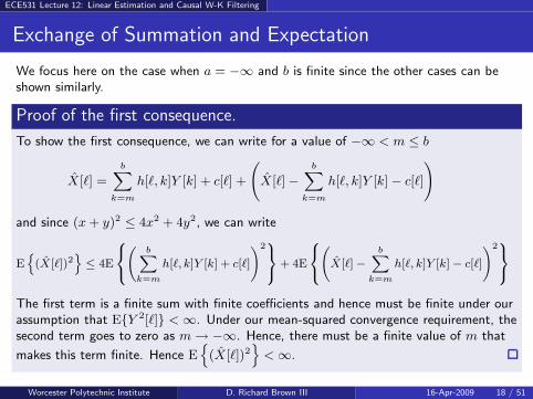
Exchange of Summation and Expectation

We focus here on the case when a = −∞ and b is finite since the other cases can beshown similarly.

Proof of the first consequence.

To show the first consequence, we can write for a value of −∞ < m ≤ b

X[ℓ] =bX

k=m

h[ℓ, k]Y [k] + c[ℓ] +

X[ℓ] −bX

k=m

h[ℓ, k]Y [k] − c[ℓ]

!

and since (x + y)2 ≤ 4x2 + 4y2, we can write

En

(X[ℓ])2o

≤ 4E

8

<

:

bX

k=m

h[ℓ, k]Y [k] + c[ℓ]

!29

=

;

+ 4E

8

<

:

X[ℓ] −bX

k=m

h[ℓ, k]Y [k] − c[ℓ]

!29

=

;

The first term is a finite sum with finite coefficients and hence must be finite under ourassumption that E{Y 2[ℓ]} < ∞. Under our mean-squared convergence requirement, thesecond term goes to zero as m → −∞. Hence, there must be a finite value of m that

makes this term finite. Hence En

(X[ℓ])2o

< ∞.



Proof of the second consequence.

To show the second consequence, we can write for a value of −∞ < m ≤ b

E{ZX [ℓ]}−

bX

k=m

h[ℓ, k]E{ZY [k]} + c[ℓ]E{Z} = E

(

Z

X[ℓ]−

bX

k=m

h[ℓ, k]Y [k] − c[ℓ]

!)

where the exchange of expectation and summation is valid since the summation is finite.The Schwarz inequality implies that the squared value of the RHS is upper bounded by

˛

˛

˛

˛

˛

E

(

Z

X[ℓ]−

bX

k=m

h[ℓ, k]Y [k]−c[ℓ]

!)˛

˛

˛

˛

˛

2

≤ E˘

Z2¯

E

8

<

:

X [ℓ]−

bX

k=m

h[ℓ, k]Y [k]−c[ℓ]

!29

=

;

A condition of the theorem is that E{Z2} < ∞. Under our mean-squared convergencerequirement, the second term on the RHS goes to zero as m → −∞. Hence the wholeRHS goes to zero and we can conclude that limm→−∞ LHS = 0, or that

E{ZX [ℓ]} =

bX

k=−∞

h[ℓ, k]E{ZY [k]} + c[ℓ]E{Z}.



Remarks

◮ The critical consequence of the theorem is that it allows us toexchange the order of expectation and summation, even when thesummations are infinite:

E{ZX[ℓ]} =

b∑

k=−∞

h[ℓ, k]E{ZY [k]} + c[ℓ]E{Z}

E{ZX[ℓ]} =

∞∑

k=a


E{ZX[ℓ]} =

∞∑

k=−∞


◮ The regularity conditions for this to hold are pretty mild:◮ E{Z2} < ∞ and E{Y [k]2} < ∞ for all k.◮ The estimator X[ℓ] must converge in a mean square sense to its limit.



The Principle of Orthogonality

Theorem

A linear estimator of the scalar state X[ℓ] is an LMMSE estimator if and

only if

E{(

X[ℓ] − X[ℓ])

Z}

= 0

for all Z that are affine functions of the observations Y [a], . . . , Y [b].

Remarks:

◮ This is a special case of the “projection theorem” in analysis.

◮ The theorem says that X [ℓ] is an LMMSE estimator (a special affinefunction of the observations Y [a], . . . , Y [b]) if and only if theestimation error X[ℓ] − X[ℓ] is orthogonal (in a statistical sense) toevery affine function of those observations.

◮ Note that the condition is both necessary and sufficient.



The Principle of Orthogonality: Geometric Intuition

space of a�ne combinations of observations

X[ℓ] − X[ℓ]

X[ℓ]

X[ℓ]



The Principle of Orthogonality

Proof part 1.

We will show that if X[ℓ] satisfies the orthogonality condition, it must be an LMMSEestimator. Suppose we have another linear estimator X[ℓ]. We can write its MSE as

E

“

X [ℓ] − X[ℓ]”2ff

= E

“

X[ℓ] − X [ℓ] + X[ℓ] − X[ℓ]”2ff

= E

“

X[ℓ] − X [ℓ]”2ff

+ 2En“

X[ℓ] − X[ℓ]”“

X [ℓ] − X[ℓ]”o

+E

“

X[ℓ] − X[ℓ]”2ff

Let Z = X[ℓ] − X[ℓ] and note that Z is an affine function of the observations. Since

X[ℓ] satisfies the orthogonality condition, the 2nd term on the RHS is equal to zero and

E

“


= E

“


+ E

“


≥ E

“


Since X [ℓ] was arbitrary, this shows that X[ℓ] is an LMMSE estimator.



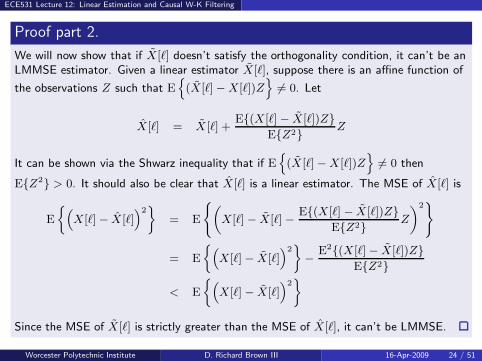
Proof part 2.

We will now show that if X[ℓ] doesn’t satisfy the orthogonality condition, it can’t be anLMMSE estimator. Given a linear estimator X[ℓ], suppose there is an affine function of

the observations Z such that En

(X[ℓ] − X[ℓ])Zo

6= 0. Let

X[ℓ] = X [ℓ] +E{(X[ℓ] − X[ℓ])Z}

E{Z2}Z

It can be shown via the Shwarz inequality that if En

(X [ℓ] − X[ℓ])Zo

6= 0 then

E{Z2} > 0. It should also be clear that X[ℓ] is a linear estimator. The MSE of X[ℓ] is

E

“

X[ℓ] − X [ℓ]”2ff

= E

(

„

X[ℓ] − X[ℓ] −E{(X[ℓ] − X [ℓ])Z}

E{Z2}Z

«2)

= E

“


−E2{(X[ℓ] − X[ℓ])Z}

E{Z2}

< E

“


Since the MSE of X[ℓ] is strictly greater than the MSE of X[ℓ], it can’t be LMMSE.



The Principle of Orthogonality Part II

Theorem

A linear estimator of the scalar state X[ℓ] is an LMMSE estimator if and

only if

E{X[ℓ]} = E{X[ℓ]}

and

E{(

X [ℓ] − X[ℓ])

Y [ℓ]}

= 0

for all a ≤ ℓ ≤ b.




Proof part 1.

We will show that if X[ℓ] is an LMMSE estimator, then it must satisfy both conditionsof PoO part II. From PoO part I, we know

E{(X [ℓ] − X[ℓ])Z} = 0 for any Z that is affine in the observations

⇒ E{(X [ℓ] − X[ℓ])1} = 0 since Z=1 is affine

⇒ E{X [ℓ]} = E{X[ℓ]}

En“

X[ℓ] − X[ℓ]”

Y [ℓ]o

= 0 for all a ≤ ℓ ≤ b is also a direct consequence of the results

from PoO part I since Y [ℓ] is an affine function of the observations Y [a], . . . , Y [b].




Proof part 2.

Now we will show that if E{X [ℓ]} = E{X[ℓ]} and En“

X [ℓ] − X[ℓ]”

Y [ℓ]o

= 0 for all

a ≤ ℓ ≤ b, then X[ℓ] must be an LMMSE estimator. Let Z =P

b

k=ag[ℓ, k]Y [k] + d[ℓ]

be an affine function of the observations. Then we have

En“

X[ℓ] − X[ℓ]”

Zo

= E

(

“

X[ℓ] − X[ℓ]”

bX

k=a

g[ℓ, k]Y [k] + d[ℓ]

!)

=bX

k=a

g[ℓ, k]En“

X[ℓ] − X[ℓ]”

Y [k]o

+ En

X[ℓ] − X[ℓ]o

d[ℓ]

= 0 + 0

Since Z is arbitrary, the results of PoO part I imply that X[ℓ] must be an LMMSEestimator.

Remark:

◮ Note that this result required an exchange of the sum and the expectation.



The Wiener-Hopf Equations

The PoO part II allows us to obtain a series of equations to specifyLMMSE estimator coefficients when we have either a finite or an infinitenumber of observations. We can immediately find the LMMSE affineoffset coefficient c[ℓ] by using the fact that E{X [ℓ]} = E{X[ℓ]}:

E

{b∑

k=a

h[ℓ, k]Y [k] + c[ℓ]

}

= E{X[ℓ]}

⇒ c[ℓ] = E{X[ℓ]} −

b∑

k=a

h[ℓ, k]E{Y [k]}

where this result requires the exchange of the order of expectation andsummation to be valid.



The Wiener-Hopf Equations

Using the fact that an LMMSE estimator must satisfy

E{(

X[ℓ] − X [ℓ])

Y [ℓ]}

= 0 for all ℓ = a, . . . , b, we can write

E

{(

X [ℓ] −

b∑

k=a

h[ℓ, k]Y [k] − c[ℓ]

)

Y [ℓ]

}

= 0 for all ℓ = a, . . . , b

Substitute for c[ℓ] and do a bit of simplification...

E

{[

X [ℓ] − E{X [ℓ]} −b∑

k=a

h[ℓ, k] (Y [k] − E{Y [k]})

]

Y [ℓ]

}

= 0

which can be further simplified to

cov(X [ℓ], Y [ℓ]) =

b∑

k=a

h[ℓ, k]cov(Y [k], Y [ℓ])

for all ℓ = a, . . . , b. Note that we exchanged the sum and the expectation order

to get the final result.Worcester Polytechnic Institute D. Richard Brown III 16-Apr-2009 29 / 51


The Wiener-Hopf Equations: Remarks

In the case of finite a and b, it isn’t difficult to show that the Wiener-Hopfequations can be written in the same form that we derived earlier:

hlmmse =[cov(Y b

a , Y b

a )]−1

cov(Y b

a , X [ℓ])

The cases when a = −∞, or b = ∞, or both a = −∞ and b = ∞ are a bitmessier, however, since we have an infinite number of Wiener-Hopf equations andcan’t form finite dimensional matrices and vectors. We can only hope to solvethese sort of problems with some further simplifying assumptions...

Simplifying assumption number 1: the (scalar) observation sequence iswide-sense stationary, i.e.,

cov(Y [ℓ], Y [k]) = CY Y [ℓ − k] = CY Y [k − ℓ]

Simplifying assumption number 2: the (scalar) observation sequence and(scalar) state sequence are jointly wide-sense stationary, i.e.,

cov(X [ℓ], Y [k]) = CXY [ℓ − k] = CY X [k − ℓ]



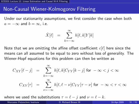
Non-Causal Wiener-Kolmogorov Filtering

Under our stationarity assumptions, we first consider the case when botha = −∞ and b = ∞, i.e.

X [ℓ] =∞∑

k=−∞

h[ℓ, k]Y [k]

Note that we are omitting the affine offset coefficient c[ℓ] here since themeans can all assumed to be equal to zero without loss of generality. TheWiener-Hopf equations for this problem can then be written as

CXY [ℓ − j] =∞∑

k=−∞

h[ℓ, k]CY Y [k − j] for −∞ < j < ∞

CXY [τ ] =

∞∑

ν=−∞

h[ℓ, ℓ − ν]CY Y [τ − ν] for −∞ < τ < ∞

where we used the substitutions τ = ℓ − j and ν = ℓ − k.Worcester Polytechnic Institute D. Richard Brown III 16-Apr-2009 31 / 51



Inspection of the Wiener-Hopf equations for the estimator X[ℓ]

CXY [τ ] =∞∑

ν=−∞

h[ℓ, ℓ − ν]CY Y [τ − ν] for −∞ < τ < ∞

reveals that the time index ℓ only appears in the coefficient sequence. Thisis a direct consequence of our stationarity assumption and implies that thefilter h[ℓ, k] doesn’t depend on ℓ (h is shift-invariant). Since ℓ is irrelevant,we can let h[ν] := h[ℓ, ℓ − ν] and rewrite the Wiener-Hopf equations as

CXY [τ ] =

∞∑

ν=−∞

h[ν]CY Y [τ − ν] for −∞ < τ < ∞

What is this? It is the discrete-time convolution of two infinite lengthsequences. We can get more insight by moving to the frequency domain...




Assuming that the discrete-time Fourier transforms exist, we can define

H(ω) =

∞∑

k=−∞

h[k]e−iωk (transfer function of h)

φXY (ω) =

∞∑

k=−∞

CXY [k]e−iωk (cross spectral density)

φY Y (ω) =∞∑

k=−∞

CY Y [k]e−iωk (power spectral density)

and the Wiener-Hopf equations become

φXY (ω) = H(ω)φY Y (ω) for all − π ≤ ω ≤ π




As long as φY Y (ω) > 0 for all −π ≤ ω ≤ π, we can solve for the requiredfrequency response of the non-causal Wiener-Kolmogorov filter as

H(ω) =φXY (ω)

φY Y (ω)

and the shift-invariant filter coefficients can be computed via the inversediscrete Fourier transform as

h[ν] =1

2π

∫ π

−π

φXY (ω)

φY Y (ω)eiων dω

for all integer ν.



Non-Causal Wiener-Kolmogorov Filtering Performance

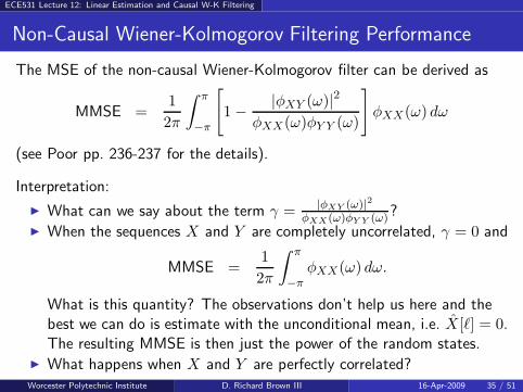
The MSE of the non-causal Wiener-Kolmogorov filter can be derived as

MMSE =1

2π

∫ π

−π

[

1 −|φXY (ω)|2

φXX(ω)φY Y (ω)

]

φXX(ω) dω

(see Poor pp. 236-237 for the details).

Interpretation:

◮ What can we say about the term γ = |φXY (ω)|2

φXX(ω)φY Y (ω)?◮ When the sequences X and Y are completely uncorrelated, γ = 0 and

MMSE =1

2π

∫ π

−π

φXX(ω) dω.

What is this quantity? The observations don’t help us here and thebest we can do is estimate with the unconditional mean, i.e. X[ℓ] = 0.The resulting MMSE is then just the power of the random states.

◮ What happens when X and Y are perfectly correlated?Worcester Polytechnic Institute D. Richard Brown III 16-Apr-2009 35 / 51


Non-Causal Wiener-Kolmogorov Filtering: Main Results

Given observations {Y [k]}∞−∞ (stationary and cross-stationary with thestates), and assuming all the discrete-time Fourier transforms exist, thenon-causal Wiener-Kolmogorov LMMSE estimator for the state X[ℓ] canbe expressed as

H(ω) =φXY (ω)

φY Y (ω)

for all −π ≤ ω ≤ π, or, equivalently,

h[ν] =1

2π

∫ π

−π

φXY (ω)

φY Y (ω)eiων dω

for all integer ν. The MSE of the non-causal Wiener-Kolmogorov filter is

MMSE =1

2π

∫ π

−π

[

1 −|φXY (ω)|2

φXX(ω)φY Y (ω)

]

φXX(ω) dω



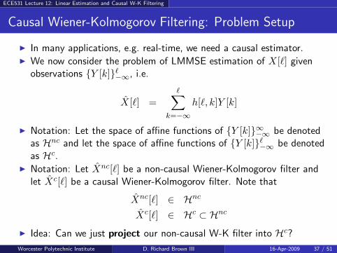
Causal Wiener-Kolmogorov Filtering: Problem Setup

◮ In many applications, e.g. real-time, we need a causal estimator.◮ We now consider the problem of LMMSE estimation of X[ℓ] given

observations {Y [k]}ℓ−∞, i.e.

X [ℓ] =ℓ∑

k=−∞

h[ℓ, k]Y [k]

◮ Notation: Let the space of affine functions of {Y [k]}∞−∞ be denotedas Hnc and let the space of affine functions of {Y [k]}ℓ

−∞ be denotedas Hc.

◮ Notation: Let Xnc[ℓ] be a non-causal Wiener-Kolmogorov filter andlet Xc[ℓ] be a causal Wiener-Kolmogorov filter. Note that

Xnc[ℓ] ∈ Hnc

Xc[ℓ] ∈ Hc ⊂ Hnc

◮ Idea: Can we just project our non-causal W-K filter into Hc?



Causal Wiener-Kolmogorov Filtering

Let Z ∈ Hc. The principle of orthogonality implies that, if Xc[ℓ] is acausal W-K LMMSE filter, then

E{

(X[ℓ] − Xc[ℓ])Z}

= 0

E{

(X[ℓ] − Xnc[ℓ] + Xnc[ℓ] − Xc[ℓ])Z}

= 0

E{

(X[ℓ] − Xnc[ℓ])Z}

+ E{

(Xnc[ℓ] − Xc[ℓ])Z}

= 0

What can we say about the first term here?

Hence E{

(Xnc[ℓ] − Xc[ℓ])Z}

= 0. What does the principle of

orthogonality imply about this result? Among all of the causal estimatorsin Hc, Xc[ℓ] is the LMMSE estimator of the non-causal Xnc[ℓ].

Implication: The causal estimator Xc[ℓ] can be obtained by first projectingX[ℓ] onto Hnc to obtain Xnc[ℓ] and then projecting Xnc[ℓ] onto Hc.



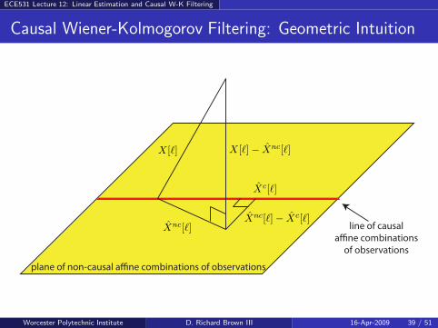
Causal Wiener-Kolmogorov Filtering: Geometric Intuition

plane of non-causal a�ne combinations of observations

line of causal

a�ne combinations

of observations

X[ℓ] − Xnc[ℓ]

Xnc[ℓ]

X[ℓ]

Xc[ℓ]

Xnc[ℓ] − Xc[ℓ]




Suppose we have our non-causal LMMSE Wiener-Kolmogorov filtercoefficients already computed as

Xnc[ℓ] =∞∑

k=−∞

hnc[ℓ, k]Y [k].

How should we perform the projection to obtain a causal LMMSEWiener-Kolmogorov filter? Let’s try this:

Xc[ℓ] =ℓ∑

k=−∞

hnc[ℓ, k]Y [k].

We are just truncating the non-causal filter to get a causal filter. How canwe check to see if this is indeed the causal LMMSE Wiener-Kolmogorovfilter? Principle of orthogonality...




By the principle of orthogonality (part II), we know that Xc[ℓ] is LMMSE if

E{

(Xnc[ℓ] − Xc[ℓ])Y [m]}

= 0 for all m = . . . , ℓ − 1, ℓ (2)

Our causal filter is just a truncation of the non-causal W-K filter, hence

Xnc[ℓ] − Xc[ℓ] =∞∑

k=ℓ+1

hnc[ℓ, k]Y [k]

One condition under which (2) holds is when the {Y [k]}∞−∞ is anuncorrelated sequence. In this case, for any m ≤ ℓ, we can write

E{

(Xnc[ℓ] − Xc[ℓ])Y [m]}

= E

{(∞∑

k=ℓ+1

hnc[ℓ, k]Y [k]

)

Y [m]

}

=∞∑

k=ℓ+1

hnc[ℓ, k]E {Y [k]Y [m]} = 0




Requiring {Y [k]}∞−∞ to be uncorrelated is a pretty big restriction on thetypes of problems we can solve. What can we do if {Y [k]}∞−∞ iscorrelated?

If we can convert {Y [k]}∞−∞ into an equivalent uncorrelated stationarysequence {Z[k]}∞−∞ by a causal linear operation, then we can determinethe causal W-K LMMSE filter by

◮ First computing the non-causal W-K LMMSE filter coefficients basedon the uncorrelated sequence {Z[k]}∞−∞ and

◮ then truncating the coefficients so that the resulting filter is causal.

Hence we need to see if we can causally and linearly whiten {Y [k]}∞−∞.



Theorem (Spectral Factorization Theorem)

Suppose {Y [k]}∞−∞

is wide-sense stationary and has a power spectrum φY Y (ω)satisfying the “Paley-Wiener condition”, given by

Z

π

−π

ln φY Y (ω) dω > −∞.

Then φY Y (ω) can be factored as φY Y (ω) = φ+

Y Y(ω)φ−

Y Y(ω) for −π ≤ ω ≤ π where

φ+

Y Y(ω) and φ−

Y Y(ω) are two functions satisfying |φ+

Y Y(ω)|2 = |φ−

Y Y(ω)|2 = φY Y (ω),

Z

π

−π

φ+

Y Y(ω)einω dω = 0 for all n < 0, (3)

andZ

π

−π

φ−

Y Y(ω)einω dω = 0 for all n > 0. (4)

Moreover (3) also holds when φ+

Y Y(ω) is replaced with 1/φ+

Y Y(ω) and (4) also holds

when φ−

Y Y(ω) is replaced with 1/φ−

Y Y(ω).



Remarks on the Spectral Factorization Theorem

◮ The Paley-Wiener condition implies that φY Y (ω) > 0 for allπ ≤ ω ≤ π, hence φ+

Y Y (ω) > 0 and φ−Y Y (ω) > 0 for all π ≤ ω ≤ π

and 1/φ+Y Y (ω) and 1/φ−

Y Y (ω) are finite for all π ≤ ω ≤ π.

◮ The inverse discrete-time Fourier transforms show that φ+Y Y (ω) has a

causal discrete-time impulse response and φ−Y Y (ω) has an

anti-causal discrete-time impulse response.

◮ The final part of the theorem implies also that 1/φ+Y Y (ω) has a

causal discrete-time impulse response and 1/φ−Y Y (ω) has an

anti-causal discrete-time impulse response.

◮ Since φY Y (ω) is a power spectral density, φY Y (ω) = φY Y (−ω) and itfollows that the spectral factors also have the property that

φ−Y Y (ω) =

[φ+

Y Y (ω)]∗

.



One Way to Whiten {Y [k]}∞−∞

◮ Recall from our discussion of the discrete-time Kalman-Bucy filterthat the innovation sequence

Y [ℓ | ℓ − 1] := Y [ℓ] − H[ℓ]X [ℓ | ℓ − 1] = Y [ℓ] − Y [ℓ | ℓ − 1]

was an uncorrelated sequence, even if the sequence {Y [ℓ]}∞−∞ iscorrelated.

◮ Note that the Y [ℓ | ℓ − 1] is not wide-sense stationary (variance istime-varying).

◮ In any case, this suggests that one practical way to build a whiteningfilter is to do one-step prediction of the observations.

◮ The only minor detail is that we need to compute a scaled innovationso that resulting sequence is stationary.



One Way to Whiten {Y [k]}∞−∞

◮ Denote the one-step causal LMMSE predictor of Y [ℓ] given the previousobservations {Y [k]}ℓ−1

−∞as

Y [ℓ | ℓ − 1] =

ℓ−1X

k=−∞

g[ℓ − k]Y [k]

and denote the MSE of this predictor as

σ2[ℓ] = E

“

Y [ℓ] − Y [ℓ | ℓ − 1]”2ff

−∞ < ℓ < ∞

◮ If we define a new sequence

Z[ℓ] =Y [ℓ] − Y [ℓ | ℓ − 1]

σ[ℓ]−∞ < ℓ < ∞

then it isn’t difficult to show that the elements of this sequence have zero mean,unit variance, and are temporally uncorrelated (using the principle of orthogonality,since the predictor is LMMSE).

◮ You can use the spectral factorization theorem to derive the causal filtercoefficients g[ν] required to implement the one-step predictor (the details are inyour textbook pp. 242-246).



Whitening

We use the fact that the spectrum at the output of an LTI filter withfrequency response G(ω) is equal to the product of the spectrum at theinput of the filter and |G(ω)|2.

At the input of the filter, we have the correlated observations Y [ℓ] withspectrum φY Y (ω). At the output of the filter, we want the equivalentsequence Z[ℓ] with constant spectrum. What should we use as our filter?

Since our whitening filter must be causal, we should use a filter withfrequency response 1

φ+

Y Y(ω)

. The spectral factorization theorem ensures

that impulse response of the filter with this frequency response is causal ifthe Paley-Wiener condition is satisfied.

What is the spectrum of Z[ℓ] in this case?




truncated

non-causal

Wiener-

Kolmogorov

whitener

1φ+(ω)

Y [ℓ]Z[ℓ]

Xc[ℓ]

Note that the non-causal Wiener-Kolmogorov filter here is based on thewhitened observations Z[ℓ]. That is,

Hnc(ω) =φXZ(ω)

φZZ(ω)for all − π ≤ ω ≤ π

We know that φZZ(ω) ≡ 1 and it can also be shown without too muchdifficulty that φXZ(ω) = G∗(ω)φXY (ω) where G(ω) = 1/φ+(ω). Hence,the non-causal Wiener-Kolmogorov filter can be expressed as

Hnc(ω) =φXY (ω)

[φ+(ω)]∗=

φXY (ω)

φ−(ω)for all − π ≤ ω ≤ π

with impulse response hnc[ν] for −∞ < ν < ∞.Worcester Polytechnic Institute D. Richard Brown III 16-Apr-2009 48 / 51



Denoting the frequency response of the causally-truncatedWiener-Kolmogorov filter (based on white observations Z[ℓ]) as

Htrunc(ω) :=

∞∑

ν=0

hnc[ν]e−iων

we now have

whitener

1φ+(ω)

Htrunc(ω)Y [ℓ]Z[ℓ]

Xc[ℓ]

Note that both filters are causal here, hence their series connection is alsocausal. The frequency response of the causal Wiener-Kolmogorov filter(based on temporally correlated observations Y [ℓ]) can then be written as

Hc(ω) =Htrunc(ω)

φ+(ω)for all − π ≤ ω ≤ π.



Final Remarks

◮ Linear estimation is motivated by◮ Computational convenience.◮ Analytical tractability.◮ No loss of optimality under MSE criterion and observations jointly

Gaussian with unknown state/parameter.

◮ We looked at (not in this order)◮ Linear MMSE with a finite number of observations (matrix-vector

formulation)◮ Kalman Filter (both static and dynamic states)◮ Linear MMSE with an infinite number of observations

⋆ Principle of orthogonality⋆ Wiener-Hopf equations⋆ Stationarity assumptions⋆ Non-causal Wiener-Kolmogorov filtering⋆ Causal Wiener-Kolmogorov filtering⋆ Spectral factorization

◮ Whitening (aka pre-whitening) is a useful tool in many applications.



Comprehensive Final Exam: What You Need to Know

◮ Everything from the first half of the course (see end of Lec. 6).

◮ Different types of parameter estimation problems (Bayesian andnon-random, static and dynamic)

◮ Mathematical model of parameter estimation problems.

◮ Bayesian parameter estimation (MMSE, MMAE, MAP, ...)

◮ Non-random parameter estimation◮ Unbiased estimators and MVU estimators.◮ RBLS theorem.◮ Information inequality and the Cramer-Rao lower bound.◮ Maximum likelihood estimators.

◮ Dynamic parameter/state estimation and Kalman filtering.

◮ Linear MMSE estimation with a finite number of observations.

Linear MMSE estimation with an infinite number of observations will notbe on the final exam.


linear estimation and causal wiener-kolmogorov filtering - spinlab

Documents