linear algebra - ndsucoykenda/linearalgebranotes.pdfchapter 1 preliminaries 1.1 basics and...

Linear Algebra

Jim Coykendall

September 13, 2004

Chapter 1

Preliminaries

1.1 Basics and Definitions

This course will cover basic graduate linear algebra. In this course we will havea view towards some algebraic K−theory (which in very loose terms can bethought of as linear algebra over a ring). The beginning of the course will bea quick overview of some of the basics of linear algebra (over a field). Includedwill be inner product spaces and some applications. We will then delve a bitinto general module theory and then specialize again to modules over a PID toget the canoncial forms of a matrix. We will end up with some basic categorytheory (on a “need to know” basis) and introduce algebraic K−theory.

In this section we will (for completeness) record some definitions and rehashsome things that we will need to know in this course.

Definition 1.1.1. A nonempty set G is said to be a group if G is equipped witha binary operation G×G −→ G (◦) such that the following hold.

a) x ◦ (y ◦ z) = (x ◦ y) ◦ z for all x, y, z ∈ G.

b) There exists e ∈ G such that e ◦ x = x ◦ e = x for all x ∈ G.

c) For all x ∈ G there exists y ∈ G such that x ◦ y = y ◦ x = e.

We note that in many instances, our groups will be abellian. That is, x◦y =y ◦ x for all x, y ∈ G (and in this case we will often write “x+ y” for “x ◦ y”).

Definition 1.1.2. A nonempty set R is said to be a ring if R is equipped withtwo binary operations (+ and ◦) such that the following hold.

a) (R,+) is an abelian group.

b) x ◦ (y ◦ z) = (x ◦ y) ◦ z for all x, y, z ∈ R.

c) x ◦ (y+ z) = x ◦ y+ x ◦ z and (x+ y) ◦ z = x ◦ z+ y ◦ z for all x, y, z ∈ R.

3

4 CHAPTER 1. PRELIMINARIES

Notationally, we will omit the ◦ notation for a ring and just write “xy”instead of x ◦ y. Additionally, we will (almost always) assume that our ring iscommutative, that is xy = yx for all x, y ∈ R. Even more frequently, we willassume that our ring has an identity (that is, an element 1R ∈ R such that1Rx = x1R = x for all x ∈ R).

Definition 1.1.3. We say that a ring, D, with identity is a division ring if thenonzero elements of D form a group under multiplication. If D is a commutativedivision ring, we say that D is a field.

Here is an important result (hand in hand with the axiom of choice) thatwill be used from time to time.

Lemma 1.1.4 (Zorn’s Lemma). Let Γ be a partially ordered set with theproperty that every chain in Γ has an upper bound (in Γ). Then Γ has a maximalelement.

Just for giggles, here is an application of Zorn’s Lemma

Theorem 1.1.5. Let R be a ring with identity. Then R has a maximal (left)ideal. What is more, any ideal I is contained in a maximal ideal M.

Proof. Let I ( R be our (left) ideal (if you merely want existence of a maximalideal you can take I = (0)). Let Γ = {J |J is a proper (left) ideal of R containing I}with the partial ordering being set-theoretic containment. Note that Gammais nonempty as I ∈ Γ.

To apply Zorn’s Lemma, we need to verify that every chain in Γ has anupper bound in Γ. Let C = {Ij} be a chain (that is, a linearly ordered subsetof Γ). We claim that U :=

⋃Ij is an upper bound for C (more precisely, the

fact that it is an upper bound is clear...we merely have to show that U ∈ Γ).To this end, we first claim that U is an (left) ideal of R. Indeed, if x, y ∈ U

then x ∈ Iα and y ∈ Iβ . Since Iα and Iβ are elements of C, then we will assumethat Iα ⊆ Iβ without loss of generality. Hence x − y ∈ Iβ ⊆ U . Showing thatrx ∈ U is similar.

To see that U is proper, note that if it is not, then 1 ∈ U and hence 1 ∈ Iαfor some α. Hence Iα is not proper which is a contradiction.

Since U is an upper bound in Γ, Zorn’s Lemma applies and hence Γ has amaximal element M. This element M is a maximal ideal of R containing I andwe are done.

We will shortly use this technique to show that every vector space has abasis. But before we put the cart before the horse, here is what a vector spaceis.

Definition 1.1.6. Let F be a field. A vector space over F is an abelian group(V,+) equipped with a scalar multiplication (a map from F × V −→ V ) suchthat for all v, w ∈ V and α, β ∈ F

a) α(v + w) = αv + αw

1.1. BASICS AND DEFINITIONS 5

b) α(βv) = (αβ)v

c) (α+ β)v = αv + βv

d) 1Fv = v.

Example 1.1.7. Standard examples of vector spaces are Rn (over R) and Cn(over R or C). Other examples of real vector spaces are Mn(R) and the real-valued functions on (a, b) (or continuous functions on (a, b)).

Example 1.1.8. The set of functions f : R −→ R is a real vector space. Canyou find a basis for this vector space?

6 CHAPTER 1. PRELIMINARIES

Chapter 2

Vector Spaces and InnerProduct Spaces

2.1 The Basics of Vector Spaces

For completeness of this chapter, we recall the definition of a vector space.

Definition 2.1.1. Let F be a field. A vector space over F is an abelian group(V,+) equipped with a scalar multiplication (a map from F × V −→ V ) suchthat for all v, w ∈ V and α, β ∈ F

a) α(v + w) = αv + αw

b) α(βv) = (αβ)v

c) (α+ β)v = αv + βv

d) 1Fv = v.

Definition 2.1.2. A subset U ⊆ V of a vector space over F is said to be asubspace, if U is an F−vector space.

Definition 2.1.3. Let V be a vector space over F and X a subset of V . Wesay the set X is linearly independent if the relation

n∑i=1

αixi = 0

(with αi ∈ F and xi ∈ X) implies that αi = 0 for all 1 ≤ i ≤ n. If the set X isnot linearly independent, we say that it is linearly dependent.

Definition 2.1.4. Let V be a vector space over the field F and X a subset ofV . We say that X spans V if every element of V can be written in the form

7

8 CHAPTER 2. VECTOR SPACES AND INNER PRODUCT SPACES

n∑i=1

αixi

with αi ∈ F and xi ∈ X.

We remark here that if X ⊆ V is a subset of the vector space V , then thesubspace spanned by X is precisely

U =⋂

W⊆V,W subspace containing X

W.

In particular, X spans V precisely when U = V .

Definition 2.1.5. Let V be a vector space and X ⊆ V a subset. We say thatX is a basis of V if X is linearly independent and X spans V .

Here is a big theorem that will help us to classify all vector spaces over anarbitrary field F.

Theorem 2.1.6. Any vector space, V , (over a division ring, D) has a basis.Additionally, any linarly independent subset of V can be expanded to a basis ofV .

Before we prove this theorem, we introduce the following lemma.

Lemma 2.1.7. Let V be a vector space over a division ring D. Then V con-tains a maximal linearly independent subset (and more generally, any linearlyindependent subset is contained in a maximal linearly independent subset).

Proof. This one has Zorn’s Lemma written all over it. We first suppose that Vis a nonzero vector space. Let v be a nonzero vector in V . As a set unto itself,{v} is a linearly independent subset of V (αv = 0 =⇒ α = 0). We let Γ be theset of all linearly independent subsets of V (partially ordered by inclusion). Bythe above remark, Γ is nonempty. We wish to apply Zorn’s Lemma, so let C bea chain in Γ. Consider the set

X =⋃B⊂C

B.

Certainly X is an upper bound for C if X is actually in Γ (that is, if X islinearly independent). To this end, suppose that

n∑i=1

αixi = 0

with αi ∈ D and xi ∈ X. But each xi ∈ C and hence (since the list of xi’sis finite and C is a chain) there is a B in the chain C such that xi ∈ B for all1 ≤ i ≤ n. But as a member of the chain, B is a linearly independent set andhence αi = 0 for all a ≤ i ≤ n. Hence Zorn’s Lemma applies and the proof

2.2. DIRECT SUMS, QUOTIENTS, AND LINEAR TRANSFORMATIONS9

is complete. (To get the parenthetical part of the Lemma, consider Γ be thecollection of linearly independent subsets of V that contain our given linearlyindependent set).

We will now use this lemma to prove the previous theorem.

Proof. To prove the theorem, we will show that a maximal linearly independentsubset of V is a basis. Let X be our maximal limearly independent subset of V(guaranteed by the previous lemma). To show that X is a basis of V , it sufficesto show that X spans V .

Suppose that X does not span V , and choose v ∈ V \ 〈X〉. Since X ismaximal with respect to being linearly independent, the set X

⋃{v} must be

linearly dependent. Hence there exists a, a1, · · · , an ∈ D and v1, · · · , vn ∈ Xsuch that

av = a1v1 + · · ·+ anvn.

Multiplying the left side by a−1 (note that a 6= 0) we obtain

v = a−1a1v1 + · · ·+ a−1anvn ∈ 〈X〉

which is a contradiction.

Corollary 2.1.8. If V is a vector space and L is a linearly independent subsetof V , then L can be expanded to a basis of V .

We end this section by defining the dimension of a vector space to be thecardinality of its basis set. Of course the basis set is not unique, but its cardi-nality is (we have not proved this, but I’ll bet that you were betting on this).We will formally record the definition.

Definition 2.1.9. Let V be a vector space over the field F. We define dimF(V ) =|X| where X is a basis for V over F.

We will formally record the following theorem and leave it as an exercise forthe reader (it is in fact an interesting exercise in set theory).

Theorem 2.1.10. Let V be a vector space and let X and Y be bases for V .Then |X| = |Y |.

2.2 Direct sums, quotients, and linear transfor-mations

In this section we will look at an important construction called the direct sumwhich will allow us to build new vector spaces from old (externally) and addi-tionally any vector space over a field can be decomposed uniquely (internally)in this fashion. We will also produce some standard results on quotient spaces


and linear transformations that are usually contained in an elementary linearalgebra course to lay the groundwork for our later generalizations.

Proposition 2.2.1. If U, V are subspaces of W then U+V = {u+v|u ∈ U, v ∈V } is a subspace of W .

This is called the sum of the subspaces U and V . We next present a way toconstruct a special kind of a sum called a direct sum.

Proposition 2.2.2. Let V and W be vector spaces over F. The abelian groupV ⊕W is a vector space with scalar multiplication given by

α(v, w) = (αv, αw)

for all v ∈ V , w ∈W and α ∈ F.

Proof. Exercise.

The difference between the sum and the direct sum is that there may besome “overlap” in a sum.

Example 2.2.3. Consider the space R3 (as an R−vector space). Let U1 =〈(1, 0, 0), (0, 1, 0)〉, U2 = 〈(0, 0, 1)〉, U3 = 〈(1, 0, 0), (0, 1, 0)〉, and U4 = 〈(0, 1, 0), (0, 0, 1)〉.R3 = U1 ⊕ U2 and R3 = U3 + U4 but R3 6= U3 ⊕ U4.

We now define the direct sum more generally.

Proposition 2.2.4. Let {Vi}i∈I be a collection of vector spaces over a fieldF. Then the abelian group ⊕i∈IVi is a a vector space with scalar multiplicationgiven by α{vi}i∈I = {αvi}i∈I .

Proof. Exercise.

A natural question is when is a vector space a direct sum of two of itssubspaces? But before we answer this we need some more technical details.

Proposition 2.2.5. Let W ⊆ V be vector spaces over F. Then the abelian groupV/W is a vector space with scalar multiplication given by α(v+W ) = αv+W .

Definition 2.2.6. Let V and W be vector spaces over F. A function φ : V −→W is called a linear transformation if

a) φ(v1 + v2) = φ(v1) + φ(v2) for all v1, v2 ∈ V and

b) φ(αv) = αφ(v) for all v ∈ V and α ∈ F.

A linear transformation is the vector space analog of an abelian group ho-momorphism. We say that a linear tranformation is surjective (onto) if it issurjective as a map of sets. We say that a linear transformation is injective(1-1) if it is injective as a map of sets. A linear transformation that is both oneto one and onto is called an isomorphism.

2.2. DIRECT SUMS, QUOTIENTS, AND LINEAR TRANSFORMATIONS11

Definition 2.2.7. Let φ : V −→ W be a linear tranformation. Then ker(φ) ={v ∈ V |φ(v) = 0} and im(φ) = {φ(v)|v ∈ V }.

Recall that φ is one to one if and only if ker(φ) = 0 and φ is onto if and onlyif im(φ) = W .

Theorem 2.2.8. Let {Ui}i∈I be subspaces of W . Then W ∼= ⊕i∈IUi if andonly if W =

∑i∈I Ui and Ui

⋂(∑i 6=j Uj) = 0 for all i 6= j.

Before we prove this, we remark that the general sum∑i∈I Ui consists of

all finite sums u1 + u2 + · · ·+ un where uk ∈ Uik .

Proof. We will prove the direction (⇐=) and leave the other direction for theenergetic reader. Suppose that W is the sum of the subspaces Ui and thatUi

⋂Uj = 0 for all i 6= j. Consider the map

φ : ⊕i∈IUi −→W

given by φ({ui}) =∑ui (note that only finitely many of the terms in this

sequence are nonzero). Since W is the sum of all of the Ui’s, this map is onto.Now suppose that {ui}i∈I ∈ ker(φ). Since only finitely many of the ui’s arenonzero (say xi1 , xi2 , · · · , xik are the nonzero entries), this means that

xi1 + xi2 + · · ·+ xik = 0.

Note that we can assume that k ≥ 2 (otherwise we are done). This equationimplies that

xi1 = −xi2 − · · · − xik ∈ Ui1⋂

(∑j 6=i1

Uj)

and hence, by assumption, xi1 = 0 which is a contradiction. This concludes theproof.

Here is a (truly wonderful) related result. This result classifies all vectorspaces over a field F.

Theorem 2.2.9. Let V be a vector space over F. Then V ∼= ⊕i∈IF. What ismore the cardinality of I coincides with the cardinality of (any) basis of V overF.

Proof. Let X = {xi}i∈I be a basis for V over F. We define a map φ : V −→⊕i∈IF by φ(

∑αixi) = {αi}i∈I . Verify that this is a linear transformation, and

is both one to one and onto.

We conclude this section with a hodge-podge of “familiar” linear algebraresults.

Proposition 2.2.10. Let V,W be vector spaces over F and φ : V −→ W alinear transformation. Then φ induces an isomorphism φ : V/ker(φ) ∼= im(φ).


Proof. Consider the map φ : V/ker(φ) −→ im(φ) given by φ(v+ker(φ)) = φ(v).To see that φ is well defined, assume that v+ ker(φ) = w+ ker(φ). This meansthat v − w ∈ ker(φ) and hence φ(v) = φ(w) and so the map is well defined. Itshould also be noted that it is straightforward that φ is onto.

To see that φ is one to one, note that φ(v+ kerφ) = 0 implies that φ(v) = 0and hence that v ∈ ker(φ). So φ is one to one.

Corollary 2.2.11. Let φ : V −→W be a linear transformation. Then dim(V ) =dim(ker(φ)) + dim(im(φ)).

Proof. Exercise.

Proposition 2.2.12. Let V and W be finite deimensional vector spaces over Fwith bases {v1, v2, · · · , vn} and {w1, w2, · · · , wm} respectively. If φ : V −→ Wis a linear transformation then φ can be represented as an element of Mm,n(F).

Proof. The important thing here is that φ is determined completely by its actionon the basis elements of V . We have the following system of equations:

φ(v1) = α1,1w1 + α2,1w2 + · · ·+ αm,1wm

φ(v2) = α1,2w1 + α2,2w2 + · · ·+ αm,2wm

...φ(vn) = α1,nw1 + α2,nw2 + · · ·+ αm,nwm

With this data in hand, it is a straightforward computations to see that them× n matrix {αi,j} 1 ≤ i ≤ n, 1 ≤ j ≤ m is the matrix that we seek.

We note here that the set of linear transformations from V to W forms avector space (over the same field, F). We will call this vector space HomF(V,W ).

Chapter 3

Inner Product Spaces

In this (brief) chapter we will look at the notion of an inner product space.In this chapter we will assume that the fields in question are either the realnumbers, R or the complex numbers C.

3.1 The basics

Definition 3.1.1. Let V be a vector space over F (= R or C). We say that Vis an inner product space if there exists a map 〈·〉 : V × V −→ F such that forall u, v, w ∈ V and α, β ∈ F we have

a) 〈u, v〉 = 〈v, u〉

b) 〈u, u〉 ≥ 0 and 〈u, u〉 = 0 if and only if u = 0

c) 〈αu+ βv,w〉 = α〈u,w〉+ β〈v, w〉.

Note that as a consequence, we have that for all λ ∈ F, 〈u, λv〉 = λ〈u, v〉.

Example 3.1.2. Consider the standard “dot product” for Rn.

Example 3.1.3. Let V = {f : [0, 1] −→ C|f is continuous.}. This is an innerproduct space with 〈f, g〉 =

∫ 1

0f(t)g(t)dt.

Note the the second property gives us a natural way to define length.

Definition 3.1.4. Let V be an inner product space and v ∈ V . We define thelength of v to be

‖v‖ =√〈v, v〉.

Note that ‖v‖ = 0 if and only if v = 0.

Lemma 3.1.5. Let V be an inner product space (over F) and let v ∈ V . Then‖αv‖ = |α| ‖v‖ for all α ∈ F.

13

14 CHAPTER 3. INNER PRODUCT SPACES

Proof. We will prove this result in the generality of the complex numbers C.Note that ‖αv‖ =

√〈αv, αv〉. But note that 〈αv, αv〉 = α〈v, αv〉 = α〈αv, v〉 =

αα〈v, v〉 = αα〈v, v〉.So we have that ‖αv‖ =

√〈αv, αv〉 =

√αα

√〈v, v〉 = |α| ‖v‖.

We are now going to produce and prove the famous Schwartz Inequality.But first we will need a lemma.

Lemma 3.1.6. Let a, b, c ∈ R with a > 0 and aλ2 + 2bλ+ c ≥ 0 for all λ ∈ Rthen b2 ≤ ac.

Proof. Set λ := − ba . By assumption we have that

b2

a− 2b2

a+ c ≥ 0.

This gives that c ≥ b2

a and hence ac ≥ b2.

Here is the Schwartz Inequality.

Theorem 3.1.7. Let V be an inner product space and u, v ∈ V , then |〈u, v〉| ≤‖u‖ ‖v‖.

Proof. We will assume without loss of generality that u 6= 0 (the theorem iseasily seen to be true in this case). We will also begin by assuming that 〈u, v〉 ∈R.

Note that for all λ ∈ R wehave that 〈λu+ v, λu+ v〉 ≥ 0. This implies thatλ2〈u, u〉 + 2λu, v〉 + 〈v, v〉 ≥ 0. Let a = 〈u, u〉, b = 〈u, v〉, c = 〈v, v〉 and applythe lemma: Since b2 ≤ ac we have that

|〈u, v〉|2 ≤ ‖u‖2 ‖v‖2

and we are done.Generally, if α = 〈u, v〉 /∈ R then α 6= 0 and so

〈 1αu, v〉 =

1α〈u, v〉 = 1 ∈ R.

Therefore we have that 1 = |〈 1αu, v〉| ≤ ‖1αu‖ ‖v‖ = ‖u‖ ‖v‖

α . Hence

α = |〈u, v〉| ≤ ‖u‖ ‖v‖

and we are done.

In the next couple of examples we will produce some applications of theSchwartz Inequality.

3.1. THE BASICS 15

Example 3.1.8. Let V = Fn (with F either R or C). Let u = (α1, · · · , αn) andv = (β1, · · · , βn). Using the standard inner product we have that

|α1β1+α2β2+· · ·+αnβn|2 ≤ (|α1|2+|α2|2+· · ·+|αn|2)(|β1|2+|β2|2+· · ·+|βn|2).

Example 3.1.9. For this example, we will let V = {f : [0, 1] −→ F|f is continuous}.We have seen that 〈f, g〉 =

∫ 1

0f(t)g(t)dt is an inner product. By the Scwartz

Inequality we have that

|∫ 1

0

f(t)g(t)dt|2 ≤∫ 1

0

|f(t)|2dt∫ 1

0

|g(t)|2dt.

Here is another geometric consequence of living in an inner product space.

Definition 3.1.10. Let V be an inner product space and u, v ∈ V . We saythat u and v are orthogonal if 〈u, v〉 = 0. We say that the set {xi} of nonzerovectors is orthogonal if 〈xi, xj〉 = 0 for all i 6= j. Additionally we say that anorthogonal set is orthonormal if 〈xi, xi〉 = 1 for all i.

This should be familiar from the “old days” of dot products.

Definition 3.1.11. Let V be an inner product space and S a subset of V . Wedefine S⊥ = {x ∈ V |〈x, s〉 = 0 for all s ∈ S}.

We record the following result.

Theorem 3.1.12. Let V be an inner product space and S a subset of V . ThenS⊥ is a subspace of V .

Proof. Exercise.

Proposition 3.1.13. Let W ⊂ V be inner product spaces. Then the followinghold.

a) V ⊆ V ⊥⊥.

b) V = V ⊥⊥⊥.

Proof. Exercise.

We will now show that a finite dimensional inner product space has anorthonormal basis. The techniques used will introduce the “Gram-Schmidt”process.

Lemma 3.1.14. If {xi} is an orthonormal set, then {xi} is a linearly inde-pendent set. Additionally, if w =

∑αixi and the set {xi} is orthonormal then

αi = 〈w, xi〉.


Proof. Suppose that r1x1 + r2x2 + · · · + rnxn = 0. This implies that 〈r1x1 +r2x2 + · · · + rnxn, xi〉 = 0. Hence ri〈xi, xi〉 = 0 and so ri = 0. This gives the“linear independence” statement.

Finally note that

〈w, xi〉 = 〈α1x1 + α2x2 + · · ·+ αnxn〉 = αi〈xi, xi〉 = αi

and we are done.

Lemma 3.1.15. If {v1, v2, · · · , vn} is an orthonormal set in V and w ∈ V then

u = w − 〈w, v1〉v1 − 〈w, v2〉v2 − · · · − 〈w, vn〉vn

is orthogonal to {v1, v2, · · · , vn}.

Proof. Exercise.

Theorem 3.1.16. Any finite dimensional inner product space has an orthonor-mal set as a basis.

Proof. Let {v1, v2, · · · , vn} be a basis for V over F. From this basis, we will usethe Gram-Schmidt process to construct an orthomormal set of n elements andthis will establish the theorem.

We begin by normalizing v1 by declaring

w1 =v1‖v1‖

.

We now let u2 = v2 − 〈v2, w1〉w1 and note that u2 ⊥ w1. Normalize againby setting

w2 =u2

‖u2‖.

Assume that we have constructed the orthonormal set {w1, w2, · · · , wm}.We let

um+1 = vm+1 − 〈vm+1, w1〉w1 − 〈vm+1, w2〉 − · · · − 〈vm+1, wm〉wm

and normalize by letting

wm+1 =um+1

‖um+1‖.

This completes the proof.

Theorem 3.1.17. Let V be a finite dimensional inner product space and W ⊆V a subspace. Then V = W ⊕W⊥.

3.1. THE BASICS 17

Proof. Note first that if z ∈W⋂W⊥ then (since z ∈W and z ∈W⊥) we have

that 〈z, z〉 = 0 and hence z = 0. So we have W⋂W⊥ = 0.

It only remains to show that W+W⊥ = V . To this end, let {w1, w2, · · · , wr}be an orthonormal basis for W , and let v ∈ V and consider

v0 = v − 〈v, w1〉 − 〈v, w2〉w2 − · · · − 〈v, wr〉wrand note that v0 ⊥ wi for all i. Hence v0 ⊥ W and hence v0 ∈ W⊥. Thisconcludes the proof.

Corollary 3.1.18. Let V be a finite dimensional inner product space and W ⊆V a subspace. Then W⊥⊥ = W .

Proof. Let w ∈ W and note that for all x ∈ W⊥ we have that 〈w, x〉 =) andhence w ∈W⊥⊥.

Also note that V = W ⊕ W⊥ = W⊥ ⊕ W⊥⊥ and hence textdim(V ) =dim(V ⊥⊥). Since V ⊆ V ⊥⊥ and dim(V ⊥⊥) is finite, we have that V = V ⊥⊥.

With inner product spaces come some nice geometry and this is one reasonthat they are so useful in analysis. We leave this chapter with a couple ofdefinitions for culture.

Definition 3.1.19. A Banach space is a vector space that is complete normedvector space.

Definition 3.1.20. A Hilbert space is a complete inner product space.

Chapter 4

Modules

4.1 Introduction and preliminaries

The theory of modules is central in the algebra and damn near everywherewhere algebra and its techniques are useful. Modules can be thought of as ageneralization of two familiar notions: the notion of a vector space and thenotion of an abelian group.

Even in the days of calculus, we saw that the study of vector and vectorspaces were essential in being able to implement the techniques of multivariablecalculus and differential equations effectively. The notion of a vector space isthe notion of a mathematical structure that is closed under addition (the sumof two vectors is a vector). More correctly the set of vectors form an abeliangroup under addition. What sets a vector space apart from an ordinary abeliangroup is the fact that the set of vectors is equipped with “scalar multiplication”where the scalars come from a field (in elementary courses, usually R or C).

The notion of an R−module is the generalization of “vector space” wherethe scalars are taken from some ring R (instead of the more specific “field”.Since a vector space and its generalization, the R−module is first and foremostan abelian group, we also think of R−modules as the generalization of abeliangroup (e.g. an abelian group equipped with ”scalar” multiplication from R).

Since the ring R need not be commutative, we will make the definition ofleft R−module first. Throughout this course there will be many theorems forleft R−modules. The reader should realize that any such theorem has an analogtheorem for right R−modules.

Definition 4.1.1. A left R− module is an abelian group (M,+) equipped witha function R ×M → M (we write (r,m) 7→ rm) such that for all r, s ∈ R anda, b ∈M we have

a) r(a+b)=ra+rb

b) (r+s)a=ra+sa

19

20 CHAPTER 4. MODULES

c) r(sa)=(rs)a

We remark here that if 1 ∈ R and 1Ra = a for all a ∈M then M is called aunitary R−module (this will be the default assumption). If R is a division ringwe call M a left vector space. As an exercise verify that 0R(a) = 0M = (r)0Mfor all r ∈ R and a ∈M .

Example 4.1.2. Note that any abelian group is a Z module. The set of con-tinuous functions from [0, 1] to R is an R−vector space. If R is any ring and Iis a left ideal of R, then I is a left R−module. (It is worth noting that Z2 is aZ− module, but not an ideal of Z.) For another example, if R ⊆ S are rings,then S is an R−module. For a more exotic example (which we will see againlater) let F be a field and V a vector space over F and T : V −→ V a lineartransformation. Then V is an F [x] module via

f(x)v = f(T )v.

Finally, we note that the analog of R is a module. More precisely, if R is aring then

⊕α∈ΛR

is an R−module with “scalar” multiplication given by

r{sα}α∈Λ = {rsα}α∈Λ.

Next we generalize the familiar notion of linear transformation (abeliangroup homomorphism).

Definition 4.1.3. Let A,B be R−modules and f : A −→ B be a function. Wesay that f is an (left) R−module homomorphism if

a) f(x+ y) = f(x) + f(y) for all x, y ∈ A.

b) f(rx) = rf(x) for all r ∈ R, x ∈ A.

If R is a division ring, then this is called a linear transformation.

Lemma 4.1.4. φ : M −→ N is an R−module homomorphism if and only ifφ(x+ ry) = φ(x) + rφ(y) for all x, y ∈M and for all r ∈ R.

Proof. Exercise.

Example 4.1.5. If A,B are any abelian groups then “Z− module homomor-phism” is synonomous with “abelian group homomorphism”.

Example 4.1.6. The function fn : Z −→ Z given by fn(x) = nx is a Z−modulehomomorphism, but not a ring homomorphism. The same is true of the func-tion g : R[x] −→ R[x] given by g(r(x)) = xr(x) (i.e., this is an R−modulehomomorphism which is not a ring homomorphism.

4.1. INTRODUCTION AND PRELIMINARIES 21

As is the case with our other morphisms, we can talk about “mono” (injec-tive), “epi” (surjective), and bijective R−module homomorphisms. The termi-nology will be analogous to earlier terminology in groups and rings.

It is important at this juncture to introduce an important class of abeliangroups that are, in certain important cases, also R−modules.

Proposition 4.1.7. Let M and N be R−modules. The set HomR(M,N) ={φ : M −→ N |φ is an R−module homomorphism.} is an abelian group (un-der pointwise addition of functions). Additionally, if R is commutative, thenHomR(M,N) is an R−module.

Proof. We will leave the fact that HomR(M,N) is an abelian group as an ex-ercise and verify the second statement. If R is commutative then we define thescalar multiplication by

(rφ)(x) = r(φ(x))

for all r ∈ R. Then it is easy to see that HomR(M,N) is an R−module.

Definition 4.1.8. Let M be a left R−module and N a subgroup of M . We saythat N is a (left) submodule of M if rN ⊆ N for all r ∈ R.

Proposition 4.1.9. Let R be a ring and M a (unitary) left R module. ThenN ⊆M is a left R−submodule of M if and only if N is nonempty and x+ry ∈ Nfor all x, y ∈ N and r ∈ R.

Proof. The necessity of the condition is straightforward. Assume that for allx, y ∈ N and r ∈ R, x + ry ∈ N . Choose r = −1 to see that for all x, y ∈ N ,x−y ∈ N . So N is an abelian group. Now choose x = 0 to see that rN ⊆ N .

Example 4.1.10. If M is a Z−module then any subgroup of M is a Z−submoduleof M .

Example 4.1.11. If f : A −→ B is an R−homomorphism, then ker(f) ={x|f(x) = 0} is an R−submodule of A. Additionally, Im(f) = {f(x)|x ∈ A} isan R−submodule of B. If C ⊆ B is an R−submodule of B then f−1(C) = {x ∈A|f(x) ∈ C} is an R−submodule of A.

Example 4.1.12. If X is a subset of some R−module, A, then 〈X〉 (theR−submodule spanned by X) is the intersection of all R−submodules of A con-taining X. That is:

〈X〉 =⋂

X⊆M⊆A

M.

If X =⋃i∈I Bi where each Bi is an R−submodule of A, then 〈X〉 is called the

sum of the Bi’s and if I = {1, 2, · · · , n} then 〈X〉 = B1 +B2 + · · ·+Bn.

We conclude this section with a special and important class of R−modules.


Definition 4.1.13. Let R be commutative with 1. An R−algebra is a ring Awith identity equipped with a ring homomorphism f : R −→ A (f(1R) = 1A)such that f(R) is contained in the center of A.

Proposition 4.1.14. If A is an R−algebra, then A is an R−module.

Proof. We define a(r) = r(a) = f(r)a. Note that 1(a) = f(1)a = 1Aa = a. Forthe second property (r + s)a = (f(r + s))a = (f(r) + f(s))a = f(r)a+ f(s)a =ra+ sa. Also (rs)a = (f(rs))a = (f(r)f(s))a = f(r)(f(s)a) = f(r)(sa) = r(sa)and finally r(a+ b) = f(r)(a+ b) = f(r)a+ f(r)b = ra+ rb.

Example 4.1.15. A good canonical example of an R−algebra is the matrix ringMn(R). The relevant homomorphism is the map that takes the element r ∈ Rto the n× n diagonal matrix with all r’s on the diagonal.

Definition 4.1.16. If A and B are R−algebras then an R−algebra homomor-phism φ : A −→ B is a ring homomorphism such that

a) φ(1A) = 1B and

b) φ(ra) = rφ(a) for all r ∈ R and a ∈ A.

4.2 Quotient Structures and the HomomorphismTheorems

The idea of quotient structure is the analog of what we have seen in the theoryof groups and rings. We begin with the following theorem.

Theorem 4.2.1. Let B,C ⊆ A be modules.

a) The quotient group A/B is an R−module with R−action given by r(a +B) = ra+B.

b) The map πB : A −→ A/B given by πB(a) = a + B is an R−modulehomomorphism with kernal B.

c) There is an R−module homomorphism B/(B⋂C) ∼= (B + C)/C.

d) If C ⊆ B then B/C ⊆ A/C and (A/C)/(B/C) ∼= A/B.

Proof. For part a) it suffices to show that the action is well-defined. Supposethat x+ B = y + B. Hence x− y ∈ B and so r(x− y) ∈ B. We conclude thatrx+B = ry+B and the action is well-defined. Showing that the multiplicationsatisfies the axioms is easy since A is an R−module. Part b) is routine. Parts c)and d) are consequences of the next theorem and we leave them for exercises.

An application of the next result is the “best way” to prove parts c) andd) of the above theorem. There are myriad others. This is called the firstisomorphism theorem.

4.3. THE DIRECT PRODUCT AND DIRECT SUM 23

Theorem 4.2.2. Let f : A −→ B be an R−module homomorphism, then finduces and R−module isomorphism

f : A/ker(f)∼= //Im(f).

Proof. Define the map

f : A/ker(f) −→ Im(f)

via f(a+ ker(f)) = f(a). Since f is an R−module homomorphism, it is easy tosee that f is as well. It is also clear that f is onto the image of f . It remains toshow that f is one to one, and so assume that f(a+ ker(f)) = 0 = f(a). Thismeans that a ∈ ker(f) and we are done.

For our last result we will produce a corollary that shows submodule corre-sponce in quotient structures.

Corollary 4.2.3. If R is a ring and B ⊆ A are R−modules then there is a 1-1correspondence between submodules of A/B and submodules of A containing B.

Proof. Let C be a submodule of A containing B. We know that from a previousresult that C/B ⊆ A/B. On the other hand, assume that M is a submodule ofA/B. Consider the canonical projection

πB : A −→ A/B.

Now consider the submodule of A: π−1B (M). Verify that M ←→ π−1

B (M)gives pur 1-1 cprrespondence.

4.3 The Direct Product and Direct Sum

As one may expect the universal constructions of direct product and direct sumhave an important analog in the theory of modules. We will see that the centraltheorems from abelian group theory carry over in this realm, and in particularwe will see later that any R−module is the homomorphic image of a particulardirect sum of special R−modules.

Theorem 4.3.1. Let {Ai}i∈I be a family of R−modules and∏i∈I Ai and

⊕i∈IAi be respectively the direct product and direct sum of the family as abeliangroups.

a) The direct product∏i∈I Ai is an R−module with R−action given by r{ai}i∈I =

{rai}i∈I .

b) The direct sum ⊕i∈IAi is an R−submodule of∏i∈I Ai with the inherited

R−action.

c) For all k ∈ I the canonical projection πk :∏i∈I Ai −→ Ak (πk({ai}) = ak)

is an R−module epimorphism.


d) For each k ∈ I the canonical injection ιk : Ak −→ ⊕i∈IAi (ιk(a) = {xi}i∈Iwhere xi = 0 if i 6= k and xk = a) is an R−module monomorphism.

Proof. The proof of this is extremely similar to the proof of the analog theoremfrom group theory.

As was the case earlier, the direct product and direct sum are (unique)solutions to certain universal mapping problems.

Theorem 4.3.2. If R is a ring, {Ai|i ∈ I} is a family of R−modules, C is anR−module and {φi : C −→ Ai|i ∈ I} is a family of R−module homomorphismsthen there is a unique R−module homomorphism φ : C −→

∏i∈I Ai such that

πiφ = φi for all i ∈ I. Additionally∏i∈I Ai is uniquely determined (up to

isomorphism) by this property.

Cφi //

φ ##FF

FF

F Ai

∏i∈I Ai

πi

OO

Proof. φ(c) = {φi(c)}i∈I is the map (verify that this is indeed an R−modulehomomorphism). Assume that ξ is another such R−module homomorphismsatisfying the universal mapping problem.

We write ξ(c) = {ci} and note that πi(ξ(c)) = ci = φi(c). Hence eachci = φi(c) and xi ≡ φ.

We will next demonstrate that the direct product is the unique (up to iso-morphism) solution to this universal mapping problem.

Assume that D is another solution to this universal mapping problem (i.e.D is an R−module that has the same properties as the direct product). Wehave the diagram:

C //

@@

@@ Ai

D

OO

in particular, replacing C with D we obtain

D //

φ AA

AA Ai

D

OO

and we note that φ = 1D is an obvious solution to this mapping problem andso φ must be precisely 1D by uniqueness.

We now consider the augmented diagram

4.3. THE DIRECT PRODUCT AND DIRECT SUM 25

Df //___

!!CCC

CCCC

C∏Ai

g //___

πi

��

D

}}{{{{

{{{{

Ai

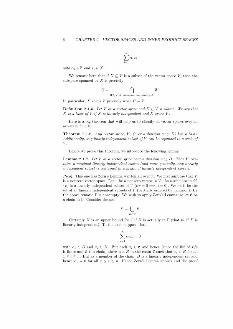
Considering the “big triangle” we see that gf = 1D must be the solutionby uniqueness. Augmenting the diagram from a different perspective (swappingthe roles of D and

∏Ai since they are both solutions to the universal mapping

problem) we get the diagram

∏Ai

g //___

!!DDD

DDDD

D Df //___

��

∏Ai

}}zzzz

zzzz

Ai

and in a similar fashion to the above, we obtain that fg = 1∏Ai

.In conclusion, we obtain that gf = 1D and fg = 1∏

Aiand hence D ∼=∏

Ai.

There is a dual result with respect the direct sum (more precisely, the directsum rears its head as the solution to the dual mapping problem).

Theorem 4.3.3. If R is a ring, {Ai|i ∈ I} is a family of R−modules, D is anR−module and {ψi : Ai −→ D|i ∈ I} is a family of R−module homomorphisms,then there is a unique R−module homomorphism ψ : ⊕i∈IAi −→ D such thatψιi = ψi for all i ∈ I. What is more, the direct sum is uniquely determined upto isomorphism by this property.

D Aiψioo

ιi

��⊕i∈IAi

ψ

ccFF

FF

F

Proof. The proof here is “dual” (e.g. essentially the same with the arrowsreversed) to the previous proof. The unique map in question is ψ({ai}) =∑i∈I ψi(ai). Note that since {ai} ∈ ⊕i∈IAi all but finitely many of the ai’s are

0 and hence the sum∑i∈I ψi(ai) is finite and “makes sense”.

We conclude this brief look at these constructions with the following result,which is a nice characterization of when an R− module is a direct sum of someof its submodules.

Proposition 4.3.4. Let R be a ring and {Ai}i∈I a family of R− submodulesof A such that

a) A is the sum of the family {Ai}.


b) For all k ∈ I, Ak⋂Ak = 0 where Ak is the sum of {Ai}i 6=k.

Then A ∼= ⊕i∈IAi.

Proof. Define φ : ⊕i∈IAi −→ A by φ({ai}) =∑i∈I ai. Since {ai} is an element

of ⊕Ai, this sum is finite. The verification that φ is an R−module homomor-phism is routine. We will show that φ is one to one and onto.

To see that φ is one to one, suppose that {ai} ∈ ker(φ) and that at least oneof the ai’s (say ak) is nonzero. We therefore have that

−ak =∑i 6=k

ai

and hence ak is an element of both Ak and the submodule of A generatedby the family {Ai}i 6=k. By assumtion, this means that ak = 0 which is ourcontradiction, and hence ker(φ) = 0.

For the onto-ness (what a word) let a ∈ A. Since the sum of the Ai’s isprecisely A, we know that there is a (finite) sum ai1 + · · ·+ aik that is equal toa. Let {xj} be the sequence defined by xi1 = ai1 , · · · , xik = aik and xj = 0 forall other indices. Note that φ({xj}) = a.

4.4 Exact Sequences

Exact sequences are the genesis of some very very important tools in commu-tative algebra, homological algebra, algebraic K-theory, and algebraic topology.Exact sequences of R−modules can contain such (seemingly) diverse informa-tion as factorization information of a commutative ring and the basic genusstructure of a topological space.

Definition 4.4.1. A sequence of R−module homomorphisms

· · · //An−1fn //An

fn+1 //An+1// · · ·

is called exact at An if Im(fn) = ker(fn+1). We say that the sequence is exactif it is exact at An for all n.

Definition 4.4.2. An exact sequence of the form

0 //Af //B

g //C //0

is called a short exact sequence (SES) if f is one to one, g is onto and ker(g) =Im(f).

As it turns out, short exact sequences are the building blocks of generalexact sequences in the following sense. If

· · · //An−1f //An

g //An+1// · · ·

4.4. EXACT SEQUENCES 27

then this sequence can be obtained by “splicing together” certain short exactsequences (as an exercise you should try to figure out how this is done).

Example 4.4.3. a) The sequence 0 //Af //B is exact if and only if f

is 1-1, the sequence Bg //C //0 is exact if and only if g is onto, the

sequence 0 //Ah //B //0 is exact if and only if h is onto.

b) If n 6= 0, the sequence 0 // Zf // Z

πn // Zn // 0 with f(k) =nk and πn(a) = a (the reduction of a modulo n) is a short exact sequence.

c) Any sequence of the form 0 //Af //A⊕ C

g //C //0 with f(a) =(a, 0) and g(a, c) = c is short exact. (It should be noted that there are usu-ally many ways to have the maps make the sequence be exact, for exampleif A = C, we could also have f(a) = (a, a) and g(x, y) = x− y). This ex-ample is a special kind of short exact sequence called a split exact sequence.Since the middle term is the sum of the second and fourth, there are mapsh : C −→ A ⊕ C such that gh = 1C and there is a k : A ⊕ C −→ A suchthat kf = 1A. In other words we could “run” the sequence in reverse. Anexample of a short exact sequence that does not split is given above in b)if n 6= 1.

We now introduce a couple of results that are fundamental if you wish toapply the concept of exactness. The proofs of most of these will be omitted asexercises, but all of them require an interesting (and fun) technique known as a“diagram chase.” This technique will be demonstrated in the proof of the shortfive lemma (but all of the diagram chase proofs are similar.

This first result is called the five lemma.

Proposition 4.4.4. Consider the following commutative diagram of R−modulehomomorphisms with exact rows

A1f1 //

g1

��

A2f2 //

g2

��

A3f3 //

g3

��

A4f4 //

g4

��

A5

g5

��B1

h1 // B2h2 // B3

h3 // B4h4 // B5

a) If g2 and g4 are onto and g5 is one to one then g3 is onto.

b) If g2 and g4 are one to one and g1 is onto then g3 is one to one.

Now we produce a corollary which is often referred to as the short five lemma.

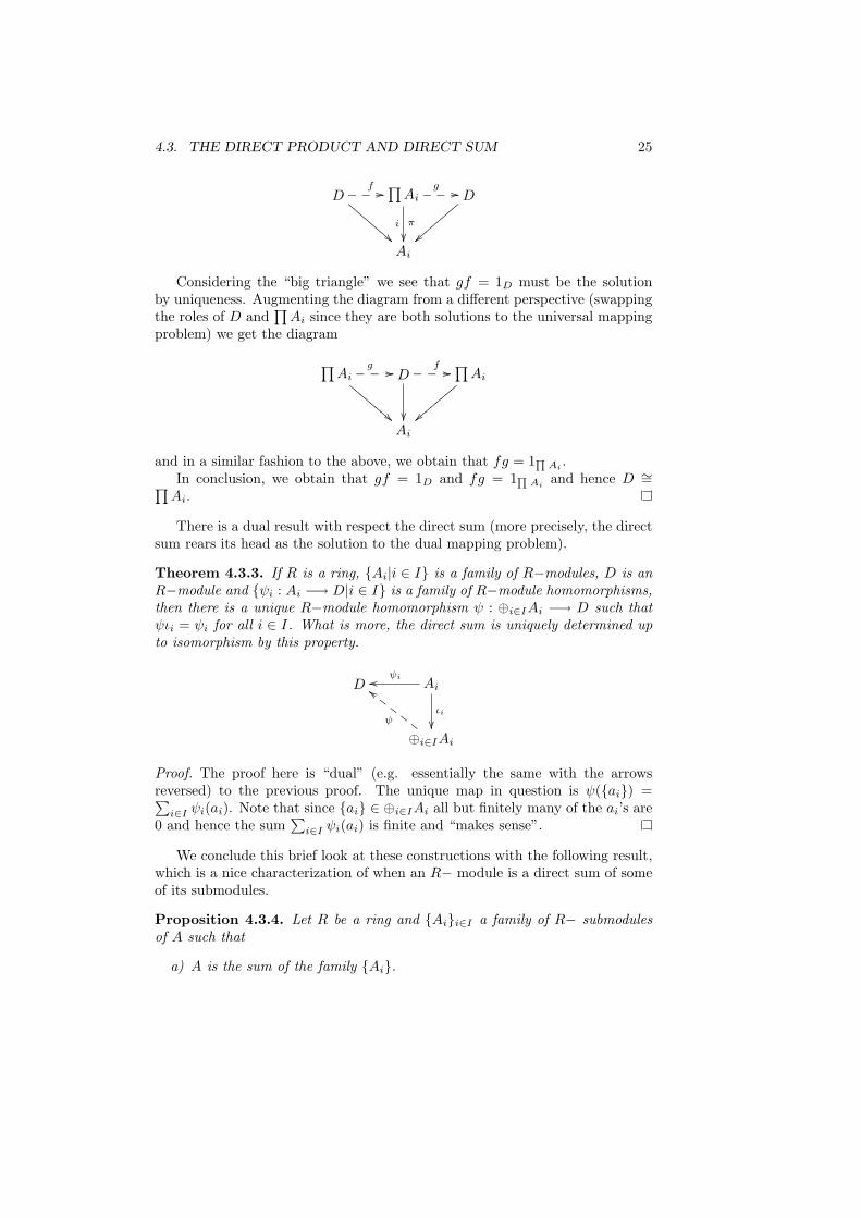
Corollary 4.4.5. Consider the following commutative diagram of R−modulehomomorphisms with exact rows


0 // A1f1 //

g1

��

A2f2 //

g2

��

A3//

g3

��

0

0 // B1h1 // B2

h2 // B3// 0

a) If g1 and g3 are onto then g2 is onto.

b) If g1 and g3 are one to one then g2 is one to one.

c) If g1 and g3 are isomorphisms that g2 is an isomorphism.

Before beginning the proof, we note that this follows directly from the fivelemma, but we will prove this result from scratch to demonstrate the techniqueof diagram chasing.

Proof. Of course c) follows directly from a) and b) so we will only show a) andb).

For a) let b2 ∈ B2. The only direction that we can go is to the left so letb3 = h2(b2) ∈ B3. Since g3 is onto, there is a a3 ∈ A3 such that g3(a3) = b3.Additionally, f2 is onto, so we can find a2 ∈ A2 such that f2(a2) = a3. Nowwe consider x = g2(a2) ∈ B2 (if x = b2 we are done, but there is no guaranteeof this). Note that by commutativity of the diagram, we have that h2(x) =b3 = h2(b2) and hence h2(b2 − x) = 0, that is, b2 − x ∈ ker(h2) = im(h1).Consequently, there is a b1 ∈ B1 such that h1(b1) = b2 − x. Now since g1 isonto there is an a1 ∈ A1 such that g1(a1) = b1, and by the commutativity ofthe diagram g2(f1(a1)) = b2 − x. Notice that y = f1(a1) ∈ A2 and g2(y+ a2) =g2(y) + g2(a2) = b2 − x+ x = b2 and hence g2 is onto.

For b) assume that a2 ∈ ker(g2), and hence g2(a2) = 0 and so h2(g2(a2)) =g3(f2(a2)) = 0 by commutativity of the diagram. Since g3 is one to one, wehave that f2(a2) = 0, so a2 ∈ ker(f2) = im(f1). So we can find (a unique,since f1 is one to one) element a1 such that f(a1) = a2. Note that g2(f1(a1)) =0 = h1(g1(a1)) Since both h1 and g1 are one to one, a1 must be 0, and hencea2 = f1(a1) = f1(0) = 0 and g2 is one to one. This completes the proof.

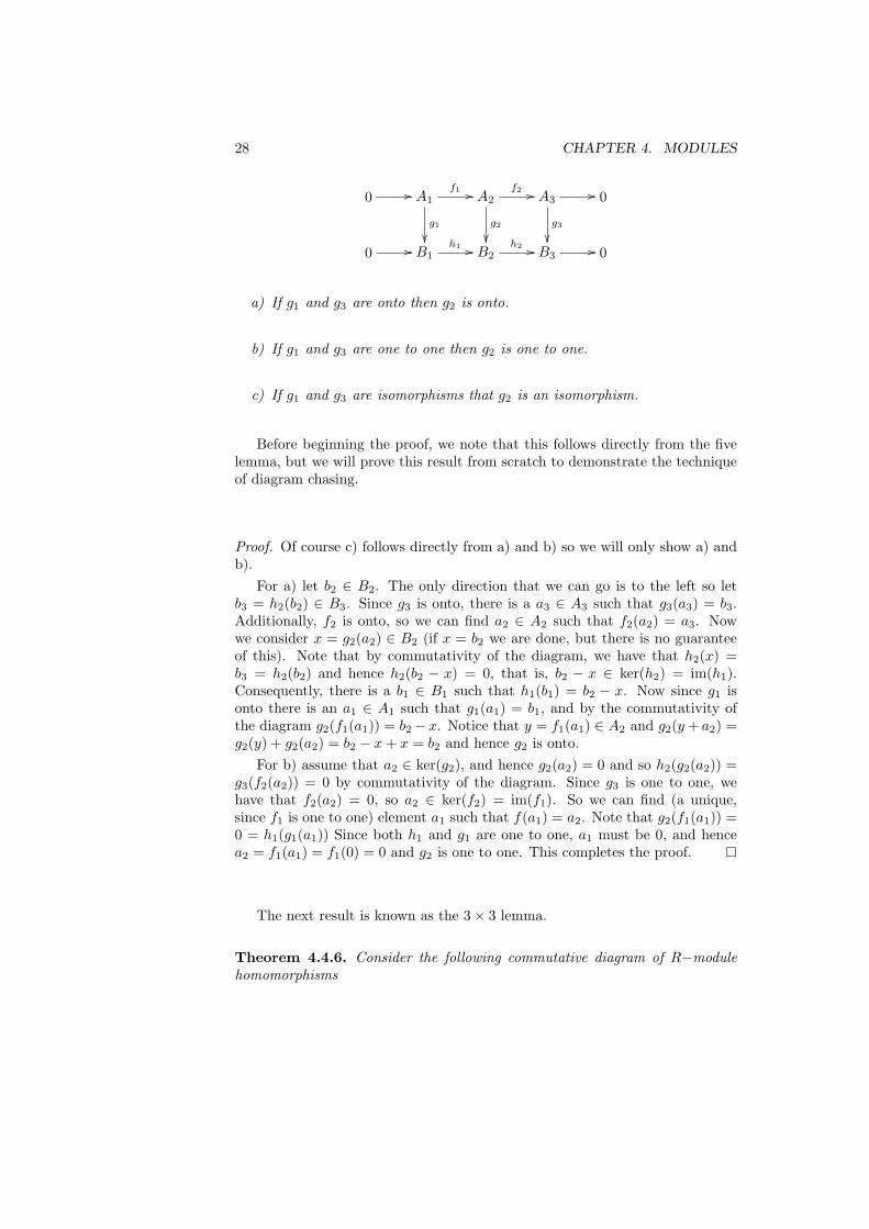
The next result is known as the 3× 3 lemma.

Theorem 4.4.6. Consider the following commutative diagram of R−modulehomomorphisms

4.4. EXACT SEQUENCES 29

0

��

0

��

0

��0 // A1

//

��

A2//

��

A3//

��

0

0 // B1//

��

B2//

��

B3//

��

0

0 // C1//

��

C2//

��

C3//

��

0

0 0 0

a) If the columns and the bottom two rows are exact, then the top row isexact.

b) If the columns and the top two rows are exact, then the bottom row isexact.

Our final “homological theorem” is the very famous snake lemma and it is oneof the major tools of homological algebra and its applications. The importantpart of the result is the existence of the well-defined homomorphism ∂ called theboundary map which allows passage from nth homology to (n− 1)th homology.

Theorem 4.4.7. Consider the following commutative diagram with exact rows

A1f1 //

g1

��

A2f2 //

g2

��

A3//

g3

��

0

0 // B1h1 // B2

h2 // B3

then there is an exact sequence

ker(g1)α1 //ker(g2)

α2 //ker(g3)∂ //coker(g1)

β1 //coker(g2)β2 //coker(g3) .

Additionally, if f1 is one to one, then so is α1 and if h2 is onto, then so is β2.

We will close out this section with a result that characterizes when a shortexact sequence is a split exact sequence.

Theorem 4.4.8. Let R be a ring and

0 //Af //B

g //C //0

a short exact sequence of R−module homomorphisms. Then the following con-ditions are equivalent.


a) There is an R−module homomorphism h : C −→ B such that gh = 1C .

b) There is an R−module homomorphism k : B −→ A such that kf = 1A.

c) B ∼= A⊕ C.

We remark that this will be our formal definition of a split exact sequence;namely a split exact sequence is a short exact sequence satisfying one, and henceall, of the above conditions.

Proof. For a)=⇒ b) we need to find an intelligent way to associate an elementof A with a given element b ∈ B. We do this by “cleaning” b. Given a b ∈ B,we are not guaranteed an element a ∈ A such that f(a) = b, so we considerhg(b) ∈ B. Note that g(b − hg(b)) = g(b) − ghg(b) = g(b) − g(b) = 0. Weconclude that b − hg(b) ∈ ker(g) = im(f). With this insight, we define k(b) =f−1(b− hg(b)). Since f is one to one, this assignment is well-defined. Supposethat f−1(b1 − hg(b1)) = a1 and that f−1(b2 − hg(b2)) = a2 and note thatf(a1 + a2) = b1 + b2 − hg(b1 + b2). Hence we have that k(b1 + b2) = f−1(b1 +b2 − hg(b1 + b2)) = a1 + a2 = k(b1) + k(b2). The proof that k(rb) = rk(b) issimilar. Note that kf(a1) = f−1(f(a1)−hgf(a1)) = f−1(f(a1)) = a1 and so a)implies b).

For b)=⇒ c) consider the map φ : B −→ A⊕ C given by φ(b) = (k(b), g(b))(verify that this is an R−module homomorphism). First let b ∈ ker(φ). So wehave k(b) = 0 and g(b) = 0. This means that b ∈ ker(g) = im(f) and so thereis an a ∈ A such that b = f(a). Therefore 0 = k(b) = k(f(a)) = a. Since a = 0,we have that b = 0 and φ is one to one.

Now let (a, c) ∈ A ⊕ C be arbitrary. Since g is onto we can select b ∈ Bsuch that g(b) = c. Unifortunately, it may not be the case that k(b) = a. Wecan, however, vary b by any element of ker(g) = im(f). Some computationsshow that the appropriate element to choose is b − fk(b) + f(a). Indeed notethat φ(b − fk(b) + f(a)) = (k(b − fk(b) + f(a)), g(b − fk(b) + f(a)) = (k(b) −kfk(b) + kf(a), g(b)) = (a, c) and φ is an isomorphism.

For now we leave c)=⇒ a) as an exercise.

4.5 Free Modules

Free modules are, in a certain sense, the easiest modules to picture (they aremost like the more familiar vector spaces). Free modules are also the “mothersof all modules” in the sense that every R−module is the homomorphic image ofa free R−module. Free modules are precisely that modules that have a notionof a basis (a very nice generating set) and we begin with the definition of abasis.

Definition 4.5.1. A subset X of an R−module M is said to be linearly inde-pendent if given any x1, x2, · · · , xn ∈ X, the relation

4.5. FREE MODULES 31

n∑i=1

rixi = 0

implies that ri = 0 for all 1 ≤ i ≤ n.

We remark (surprise, surprise) that a set that is not linearly independent iscalled linearly dependent. Also if M is generated by X, we say that X spansM . Finally we tie these together by saying that a linearly independent subset ofM that spans M (if such a subset of M exists) is called a basis of M . Moduleswhich actually have a basis are free modules that we have been alluding to.

Theorem 4.5.2. Let R be a ring with identity and F a unitary R−module.The following conditions are equivalent.

a) F has a nonempty basis.

b) F is the (internal) direct sum of a family of cyclic R−modules each ofwhich is isomorphic to R as an R−module.

c) F is R−module isomorphic to a direct sum of some number of copies ofthe R−module R.

d) There exists a nonempty set X and a function ι : X ↪→ F such thatgiven any unitary R−module M and function f : X −→ M , there existsa unique R−module homomorphism f : F −→M such that fι = f .

Ff //___ M

X

ι

OO

f

>>}}}}}}}}

Proof. We first consider a) implies b). Let X be a basis of F . Note that ifx ∈ X then R ∼= Rx as a left R−module (since the singleton set {x} is linearlyindependent). Also note that F =

∑x∈X Rx (but the sum may not be direct

and that is what we need to show). Suppose that m ∈ Rx⋂

(∑y∈X\xRy) then

we can write

rx =∑

riyi

and hence the set X is linearly dependent.The implication b) implies c) is easy and is left to the reader.

For c) implies d) let F ⊕ Ri with each Ri isomorphic is R via Riφi //R .

So (for all i we have the commutative diagram

Riφi //

ιi

��

R

F ∼= ⊕Ri

::vvvvvvvvvv


Define X = {xi}i∈I where xi is such that φi(xi) = 1R. So our function iota :X −→ F assigns to each cyclic generator its image in F . That is ι(xi) = ιi(xi)and say that f : X −→M makes the assignment f(xi) = mi ∈M . The desiredhomomorphism is the homomorphism that obeys the rule:

f(∑

riιi(xi)) =∑

rimi

and uniqueness is an easy exercise.We leave the last implication to the reader.

Here is an important corollary that reflects the universal nature and impor-tance of free modules.

Corollary 4.5.3. Every unitary module M over a ring with identity is thehomomorphic image of a free R−module. In fact, if M is finitely generated,then the free module may be chosen to be finitely generated.

Proof. Let X be a generating set of M and consider the diagram

Ff //____ M

X

ι

OO

f=inclusion

<<xxxxxxxxxfι = f

In the diagram above the module F is free on the set X (note that if Xis finite then F is finitely generated). We have an induced homomorphismf : F −→ M and X ⊂ im(f) therefore since X is a generating set, im(f) = Mand this gets the first statement. Also as was pointed out earlier, if M is finfitelygenerated (that is, X my be chosed to be finite) then F is finitely generated.

Here we do a little specialization to the case of vector spaces.

Lemma 4.5.4. A maximal linearly independent subset of a vector spcae V overa division ring D is a basis of V .

Proof. Let X be a maximal linearly independent subset (how do we know suchan animal exists...we don’t yet, but will later see that in important cases thesedo exist). Let W be a subspace of V spanned by X. If W = V then we aredone so we selesct a ∈ V \W . Of course {a}

⋃X must be linearly dependent,

so we have an equation of the form

ra+∑

rixi = 0

with xi ∈ X, r, ri ∈ R and r 6= 0 (if the last condition does not hold then thelinear independence of the set X would force all of the ri’s to be 0 as well).

Manipulating this equation gives us that

a =∑−r−1rixi ∈ V

4.5. FREE MODULES 33

which is a contradiction. Hence there is no a ∈ V \W and so V = W and weare done.

Here is a big module structure theorem for modules over a division ring(vector spaces). This is why “linear algebra” is much easier that modules ingeneral...over a field modules are always free.

Theorem 4.5.5. Every vector space V over a division ring D has a basis andis therefore free. More generally, every linearly independent subset of V is con-tained in a basis of V .

Before we prove this theorem, we also remark that if every unitary moduleover a ring with identity, D, is free, then D is a division ring.

We also point out that this business about “every linearly independent subsetof V is contained in a basis for V ” does not extend to free modules over a generalring. Indeed if you consider the simple example of Z as a Z module, consider themaximal linearly independent subset {2}. This set is not contained in a basisfor Z, because any two element subset of the integers is linearly independent.The problem here is that {2} does not span Z and we immediately see thecontrasting situation of a ring not being a division ring (i.e., we can see that wesomehow need 1

2 to be an integer for the set {2} to have a chance of spanningZ).

Proof. We will prove the more general statement and capture it all at once.Suppose that X is a linearly independent subset of V (note that such a

set has to exist in a nonzero vector space). Consider the collection of linearlyindependent subsets of V that contain X (and we will call it Γ). This is apartially ordered set under inclusion. Let {Ci} be a chain in Γ. Note thatC =

⋃i Ci is linearly independent (verify!) and hence is an upper bound for

the chain in Γ. Thus Zorn’s Lemma gives the existence existence of a maximalelement and this establishes the theorem.

Remark 4.5.6. If R is a ring that has a division ring as a homomorphic image(e.g. any commutative ring with identity), then R has the invariant dimensionproperty. That is for any free module F over R, any two bases have the samecardinality. If R has the invariant dimension property, then two free modules Eand F are isomorphic if and only if they have the same rank. For an exampleof a ring which does not have the invariant dimension property consider K, afield, and F = ⊕∞n=1K. If R = HomK(F, F ). For any n, R ∼= ⊕nm=1R (checkthis).

In closing we look at a couple of familiar properties of vector spaces. Theproofs are left as exercises.

Theorem 4.5.7. Let W be a subspace of V .

a) dimD(W ) ≤ dimD(V ).

b) If dimD(W ) = dimD(V ) and dimD(V ) is finite, then W = V .


c) dimD(V ) = dimD(W ) + dimD(V/W ).

d) If f : V −→W is a linear transformation then dimD(V ) = dimD(ker(f))+dimD(im(f)).

e) If V and W are finite dimensional then dimD(V )+dimD(W ) = dimD(V⋂W )+

dimD(V +W ).

Example 4.5.8. Build a 2× 2 matrix and examine the above theorem.

4.6 Projective and Injective Modules

We will define and prove some of the analogous results for projectives and injec-tives. Please note the “dual” (arrow reversing) nature of some of the definitionsand results. For many projective (respectively injective) results there is a verysimilar injective (resp. projective) result.

Definition 4.6.1. Consider the following diagram of R−modules with the bot-tom row exact.

Ph

��~~

~~

f

��A g

// B // 0

We say that P is projective if there is an R−module homomorphism h : P −→ Asuch that gh = f .

Definition 4.6.2. Consider the following diagram of R−modules with the toprow exact.

0 // Ag //

f

��

B

h��~~

~~

I

We say that I is injective if there is an R−module homomorphism h : B −→ Isuch that hg = f .

We will now investigate some of the consequences of these definitions intandem.

Theorem 4.6.3. Every (unitary) free module over R is projective.

Proof. Consider the following diagram

F

f

��A g

// B // 0

4.6. PROJECTIVE AND INJECTIVE MODULES 35

Let F be free on the set X (and we will denote the canonical injection fromX into F by ι : X ↪→ F ). Since g is onto, there is ai ∈ A such that g(ai) = fι(xi)for all i. Therefore we have a function f∗ : X −→ A such that f∗(xi) = ai.Since F is free, this induces an R−module homomorphism h : F −→ A suchthat hι(xi) = ai. Therefore ghι(xi) = g(ai) = fι(xi) and hence gh = f . HenceF is projective.

Definition 4.6.4. Let D be an abelian group. We say that D is divisible ifgiven d ∈ D and 0 6= n ∈ Z, there exists a d′ ∈ D such that nd′ = d.

Basically, in a divisible group we can divide by any nonzero integer.

Lemma 4.6.5. D is divisible if and only if D is an injective Z−module.

Proof. (⇐=) Let D be injective and d ∈ D and n be a nonzero integer. Considerthe diagram

0 // 〈n〉 ⊆ //

f

��

Z

h~~~~

~~

D

Let d′ = h(1) and therefore nd′ = nh(1) = h(n) = f(n) = d and hence D isdivisible.

The other direction is an exercise.

Note that in the parallel results coming up many of the proofs are dual (insome places the proofs are more different).

Theorem 4.6.6. The following conditions on the R−module P are equivalent.

a) P is projective.

b) Every short exact sequence of the form 0 //A //B //P //0 issplit exact.

c) There is an R−module K and a free module F such that F ∼= P ⊕K.

Theorem 4.6.7. The following conditions on the R−module I are equivalent.

a) I is injective.

b) Every short exact sequence of the form 0 //I //B //C //0 issplit exact.

c) I is a direct summand of any module of which it is a submodule.

Proof. We will provide a proof of the projective result. Try to do the injectiveone yourself.

For a) implies b) consider the short exact sequence 0 //Af //B

g //P //0.We now consider the diagram


Ph

��~~

~~

1P

��B g

// P // 0

Since P is projective, there exists h : P −→ B such that gh = 1P , and hencethe short exact sequence splits.

For b) implies c), we assume b) and assume that P is our given projectivemodule. We know that any R module is the homomorphic image of a free

module F (i.e. we have the onto map Fφ //P //0. Hence we have the

short exact sequence

0 //ker(φ) //Fφ //P //0.

Since the sequence must split, we have that F ∼= P ⊕ ker(φ) and we haveestablished b) implies c).

For the implication c) implies a) consider the following diagram.

P

g

��B

f// P // 0

Keeping in mind that there is a free module F with F ∼= K ⊕P , we expand thediagram

F ∼= K ⊕ P

π

��h∗

��

��

��

��

P

ι

OO

g

��A

f// B // 0

where π(k, p) = p and ι(p) = (0, p) (note πι = 1P ). Since any free module isprojective there is an h∗ : F −→ A such that fh∗ = gπ. Now consider the mapP −→ A given by h∗ι. Note that f(h∗ι) = gπι = g and hence P is projective.

We note here the the proof of the dual injective theorem requires the resultthat will be recorded later that says that every R−module can be embedded inan injective R−module.

Corollary 4.6.8. Let {Pi}i∈I be a family of R−modules. ⊕i∈IPi is projectiveif and only if Pi is projective for all i ∈ I.

4.7. HOM 37

Proof. If each Pi is projective, then for all i there is a Qi such that Qi ⊕ Pi isfree. Hence we have the free module

⊕i∈I(Pi ⊕Qi) ∼= (⊕i∈IPi)⊕ (⊕i∈IQi)

and hence the module ⊕i∈IPi (being the summand of a free module) is projec-tive.

On the other hand, assume that ⊕i∈IPi ∼= Pi⊕ (⊕j 6=iPj is projective. So wecan find an R−module K so that K⊕i∈IPi is free and hence Pi⊕(K⊕(⊕j 6=iPj))is free and hence Pi is projective.

Corollary 4.6.9. Let {Ij}j∈Γ be a family of R−modules.∏j∈Γ Ij is injective

if and only if Ij is injective for all i ∈ Γ.

Proof. Very similar to the previous. Exercise.

Corollary 4.6.10. Every R−module is the homomorphic image of a projectiveR−module.

Proof. Any free is projective.

Theorem 4.6.11. Every R−module M can be embedded in an injective R−module.

Proof. Exercise. As a hint, first show that M (considered as an abelian group)can be embedded in a divisible abelian groupD. Now embedM (as anR−module)in the R−module HomZ(R,D).

4.7 Hom

The notation HomR(A,B) will denote the set of R−module homomorphismsf : A −→ B. The is an abelian group under the standard addition (and notethat the addition respects the standard function composition of R−module ho-momorphisms.

We consider R−module homomorphisms γ : C −→ A and ξ : B −→ D. Themap η : HomR(A,B) −→ HomR(C,D) given by

f 7→ ξfγ

is an R−module homomorphism. We call this the homomorphism induced byξ and γ. Note that if B = D and ξ = 1D, then the map is f 7→ fγ (denotedγ). If A = C and γ = 1A then the map is f 7→ ξf (and is denoted ξ). We willmotly be considering these special cases.

Theorem 4.7.1. Let R be a ring. The sequence 0 //Af //B

g //C isexact if and only if for all R−modules D the sequence

0 //HomR(D,A)f //HomR(D,B)

g //HomR(D,C)


is exact.

Additionally Af //B

g //C //0 is exact if and only if for every R−moduleD the sequence

0 //HomR(C,D)g //HomR(B,D)

f //HomR(A,D)

is exact.

We say that the “Hom functor” is left exact.We will prove the first statement and leave the proof of the second as an

exercise.

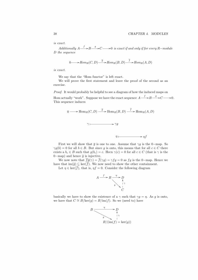
Proof. It would probably be helpful to see a diagram of how the induced maps on

Hom actually “work”. Suppose we have the exact sequence Af //B

g //C //0.This sequence induces

0 // HomR(C,D)g // HomR(B,D)

f // HomR(A,D)

γ � // γg

η � // ηf

First we will show that g is one to one. Assume that γg is the 0−map. Soγg(b) = 0 for all b ∈ B. But since g is onto, this means that for all c ∈ C thereexists a bc ∈ B such that g(bc) = c. Hecn γ(c) = 0 for all c ∈ C (that is γ is the0−map) and hence g is injective.

We now note that fg(γ) = f(γg) = γfg = 0 as fg is the 0−map. Hence wehave that im(g) ⊆ ker(f). We now need to show the other containment.

Let η ∈ ker(f), that is, ηf = 0. Consider the following diagram

Af // B

g @

@@@@

@@η // D

C

γ

OO��

basically we have to show the existence of a γ such that γg = η. As g is onto,we have that C ∼= B/ker(g) = B/im(f). So we (need to) have

B

g ''OOOOOOOOOOOOOη // D

B/(im(f) = ker(g))

γ

OO��

4.7. HOM 39

We define γ by γ(b + ker(g)) = η(b). Note if b ∈ ker(g) = im(f) thenη(b) = ηf(a) = 0 so this map is well-defined. It is also easy to verify that this isa homomorphism. Finally note that the diagram commutes since if b ∈ B thenγg(b) = γ(g(b) + ker(g)) = η(b).

This shows that the exactness of the original sequence gives the exactnessof the “Hom” sequence. The other direction is an exercise.

Example 4.7.2. Hom the sequences of Z−modules 0 //Z 2 //Z //Z2//0

and 0 //Z incl //Q //Q/Z //0 .

We will see in the next thereom that split exact sequences are decidedlymore well-behaved.

Theorem 4.7.3. The following conditions on R−modules are equivalent.

a) 0 //Af //B

g //C //0 is split exact.

b) 0 //HomR(D,A)f //HomR(D,B)

g //HomR(D,C) //0 is split ex-act for every D.

c) 0 //HomR(C,D)g //HomR(B,D)

f //HomR(A,D) //0 is split ex-act for every D.

Proof. We will show the equivalence of a) and c), the other equivalence beingleft as an exercise.

For the implication a) implies b) if suffices to show that there is an h suchthat gh is the identity on HomR(D,C). Since the original sequence is split exactthere exists h : C −→ B such that gh = 1C . It is easy to see that the inducedhomomorphism gh = gh = 1HomR(D,C) hence g is onto and the Hom sequenceis split exact.

On the other hand, assume that the Hom sequence is split exact for all D.Let D = C and φ : C −→ B be such that g(φ) = 1C = gφ. Note that this

implies that 0 //A //Bg //C //0 is split exact. The equivalence of

a) and c) is similar.

Theorem 4.7.4. The following conditions on the R−module P are equivalent.

a) P is projective.

b) If φ : B −→ C is onto then φ : HomR(P,B) −→ HomR(P,C) is onto.

c) If 0 //Aψ //B

φ //C //0 is a short exact sequence then

0 //HomR(P,A)ψ //HomR(P,B)

φ //HomR(P,C) //0 is a shortexact sequence.


Theorem 4.7.5. The following conditions on the R−module I are equivalent.

a) I is injective.

b) If ξ : A −→ B is one to one then ξ : HomR(B, I) −→ HomR(A, I) is onto.

c) If 0 //Aξ //B

η //C //0 is a short exact sequence then

0 //HomR(C, I)η //HomR(B, I)

ξ //HomR(A, I) //0 is a shortexact sequence.

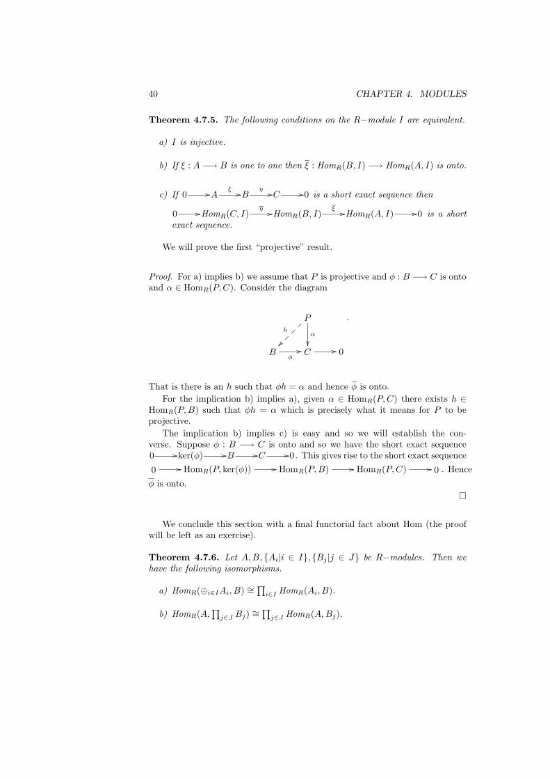
We will prove the first “projective” result.

Proof. For a) implies b) we assume that P is projective and φ : B −→ C is ontoand α ∈ HomR(P,C). Consider the diagram

Ph

��~~

~~

α

��B

φ// C // 0

.

That is there is an h such that φh = α and hence φ is onto.For the implication b) implies a), given α ∈ HomR(P,C) there exists h ∈

HomR(P,B) such that φh = α which is precisely what it means for P to beprojective.

The implication b) implies c) is easy and so we will establish the con-verse. Suppose φ : B −→ C is onto and so we have the short exact sequence0 //ker(φ) //B //C //0. This gives rise to the short exact sequence

0 // HomR(P, ker(φ)) // HomR(P,B) // HomR(P,C) // 0 . Hence

φ is onto.

We conclude this section with a final functorial fact about Hom (the proofwill be left as an exercise).

Theorem 4.7.6. Let A,B, {Ai|i ∈ I}, {Bj |j ∈ J} be R−modules. Then wehave the following isomorphisms.

a) HomR(⊕i∈IAi, B) ∼=∏i∈I HomR(Ai, B).

b) HomR(A,∏j∈J Bj) ∼=

∏j∈J HomR(A,Bj).

4.8. THE TENSOR PRODUCT 41

4.8 The Tensor Product

Although it can be done in much more generality, here we will (at least beginwith) the tensor product of modules over a commutative ring with identity.The tensor product can be done in the more general case (but care must betaken using left, right, and bi-modules when necessary). The tensor productis a universal construction (it is the solution to a certain univeral mappingproblem involving bilinear maps) and it crops up all over commutative algebraand mathematics in general (Einstein used them for example).

Definition 4.8.1. Let A,B,C be R− modules. A bilinear map F : A×B −→ Cis a function such that for all a, ai ∈ A, b, bi ∈ B and r ∈ R we have

a) f(a1 + a2, b) = f(a1, b) + f(a2, b).

b) f(a, b1 + b2) = f(a, b1) + f(a, b2).

c) f(ra, b) = f(a, rb) = rf(a, b).

We now define the tensor product of two modules.

Definition 4.8.2. Let A and B be modules over R and let F be the free abeliangroup on the set A × B. Let K be the subgroup of F generated by all elementsof the form

a) (a1 + a2, b)− (a1, b)− (a2, b)

b) (a, b1 + b2)− (a, b1)− (a, b2)

c) (ra, b)− (a, rb)

where a, a1, a2 ∈ A, b, b1, b2 ∈ B and r ∈ R.The quotient F/K is called the tensor product (over R) of A and B and is

denoted A⊗R B.

We denote the coset (a, b) +K by a⊗ b (and this is called a tensor). Prac-tically, think of A ⊗R B as generated by tensors of the form a ⊗ b subject thethe relations a), b), and c) above.

We also point out that the map ι : A×B −→ A⊗RB given by (a, b) 7→ a⊗bis a bilinear map (verify this).

Here is a theorem which shows where tensor product “came from.” Thistheorem shows that the tensor product is the unique solution to a mappingproblem concerning bilinear maps.

Theorem 4.8.3. If A,B,C are R−modules and g : A× B −→ C is a bilinearmap then there exists a unique R−module homomorphism g : A ⊗R B −→ Csuch that gι = g (where ι(a, b) = a⊗ b is the canonical bilinear map). A⊗R Bis uniquely determined up to isomorphism by this property.


A⊗R Bg //___ C

A×B

ι

OO

g

;;wwwwwwwww

Proof. Let F be free abelian on A × B and K the subgroup described above.The map g : A×B −→ C is bilinear and induces a homomorphism g∗ : F −→ C.The fact that g is bilinear shows that g∗ takes every element of K to 0 (that is,K ⊆ ker(g∗)). So g∗ induces g : F/K −→ C, that is g : A ⊗R B −→ C. Notethat gι(a, b) = g(a⊗ b) = g(a, b) and hence gι = g.

Now if h : A⊗R B −→ C is another such homomorphism then

h(a⊗ b) = g(a, b) = g(a⊗ b)

and hence h and g agree on tensors. Therefore h = g.

Here is a useful corollary which we will be building upon.

Corollary 4.8.4. Let A,A′, B,B′ be R−modules and f : A −→ A′ and g :B −→ B′ be R−module homomorphisms, then there exists a unique homomor-phism

A⊗R B −→ A′ ⊗B′

such that a⊗ b 7→ f(a)⊗ g(b) for all a ∈ A and b ∈ B.

Proof. One merely needs to verify that (a, b) 7→ (f(a)⊗ g(b)) is a bilinear map.

This next result is the “right exactness” of tensor product.

Theorem 4.8.5. If D is an R−module then −⊗RD is right exact. That is, if

Af //B

g //C //0

is exact, then so is

A⊗R Df⊗1D //B ⊗R D

g⊗1D //C ⊗R D //0

Proof. Since g is onto, every generator c⊗d of C⊗RD is of the form g(b)⊗d =(g⊗ 1D)(b⊗ d) and hence every generator of C ⊗RD is in the image of g⊗ 1D.So g ⊗ 1D is onto.

Now note that (g⊗ 1D)((f ⊗ 1D)(∑ni=1(ai ⊗ di))) = (g⊗ 1D)(

∑ni=1(f(ai)⊗

di) =∑ni=1(gf(ai)⊗ di). Since gf = 0, we have that this is a sum of zeros and

hence im(f ⊗ 1D) ⊆ ker(g ⊗ 1D).For the last bit, we have to show that ker(g ⊗ 1D) ⊆ im(f ⊗ 1D). To this

end we consider

π : B ⊗R D −→ (B ⊗R D)/(im(f ⊗ 1D)

4.8. THE TENSOR PRODUCT 43

and we note that there exists a homomorphism ξ : (B ⊗R D)/(im(f ⊗ 1D) −→C ⊗R D such that ξ(π(b⊗ d)) = (g ⊗ 1D)(b⊗ d) = g(b)⊗ d. It suffices to showthat ξ is an isomorphism.

Consider η : C ×D −→ (B ⊗R D)/(im(f ⊗ 1D) given by (c, d) 7→ π(b ⊗ d)where g(b) = c. (Note if g(b1) = c then g(b − b1) = 0 and there is an a ∈ Asuch that f(a) = b− b1; since f(a)⊗ d ∈ im(f ⊗ 1D, π(f(a)⊗ d) = 0 and henceπ(b ⊗ d) = π((f(a) + b1) ⊗ d) = π(b1 ⊗ d) and so the map is well-defined). Itis easy to see that η is bilinear and so there exists a unique eta : C ⊗R D −→(B⊗RD)/im(f ⊗ 1D) such that η(c⊗ d) = π(b⊗ d). Hence given any generatorc× d, we have

ξη(c⊗ d) = ξ(π(b⊗ d)) = g(b)⊗ d = c⊗ d

and hence ξη is the identity. In a similar fashion ηξ is the identity and the proofis complete.

Theorem 4.8.6. There is an R−module isomorphism

A⊗R R ∼= A.

Proof. The assignment (a, r) = ra is a bilinear map and so we obtain theR−module homomorphism f : A ⊗R R −→ A with f(a ⊗ r) = ra. We nowconsider the R−module homomorphism g : A −→ A⊗RR given by g(a) = a⊗1.Note that gf = 1A⊗RR and fg = 1A, and hence f is an isomorphism.

Other properties such as (adjoint) associativity will be discussed in exercises.We end with a couple of theorems concerning the behavior of tensor productwith free modules.

Theorem 4.8.7. Let A,Ai, B,Bj be R−modules. Then there are isomorphisms

a) (⊕i∈IAi)⊗R B ∼= ⊕i∈I(Ai ⊗R B).

b) A⊗R (⊕j∈JBj) ∼= ⊕j∈J(A⊗R Bj).

Proof. For a) consider the bilinear map ({ai}, b) 7→ {ai ⊗ b} (note that almostevery ai = 0). Show this induces the relevant isomorphism. The proof for b) issimliar.

Corollary 4.8.8. Let F be a free R−module then

F ⊗R B ∼= ⊕i ∈ IB

where |I| = rank(F ).

Proof. Note that F ⊗R B ∼= (⊕i∈IR)⊗R B ∼= ⊕i∈I(R⊗R B) ∼= ⊕i∈IB.


4.9 Flatness

Flatness is a certain generalization of freeness (and projectivity). A flat moduleis a module that makes tensoring exact. More precisely, we have the followingdefinition.

Definition 4.9.1. We say that the R−module M is flat if given any short exactsequence

0 //Af //B

g //C //0

the corresponding sequence

0 //A⊗RMf⊗1M //B ⊗RM

g⊗1M //C ⊗RM //0

is exact.

We note that since tensoring gets you “most” of the exact sequence for freeanyway, an equivalent characterization of a flat module M is one for which givenany one to one map f : A −→ B, the corresponding map f ⊗ 1M : A⊗RM −→B ⊗RM is one to one.

Here is a theorem that we record to show the pecking order.

Theorem 4.9.2. Let M be an R−module. For the following list of properties,we have the implications a) =⇒ b) =⇒ c).

a) M is free.

b) M is projective.

c) M is flat.

We leave the proof of the previous result and the next corollary as exercises.

Corollary 4.9.3. Let Mi be a family of R−modules. ⊕i∈IMi is flat if and onlyif Mi is flat for each i.

Bibliography

45

linear algebra - ndsucoykenda/linearalgebranotes.pdfchapter 1 preliminaries 1.1 basics and...

Documents