linear algebra and the basic mathematical tools for finite ...echitamb/teaching/phys476q/dirac...
TRANSCRIPT
PHYS 476Q: An Introduction to Entanglement Theory (Spring 2018)Eric Chitambar
Linear Algebra and the Basic Mathematical Tools forFinite-Dimensional Entanglement Theory
Quantum mechanics describes nature in the language of linear algebra. In this lecture, we willreview concepts from linear algebra that will be essential for our study of quantum entanglement.Our focus here is on finite-dimensional vector spaces since all physical systems that we considerin this course are finite-dimensional.
Contents
1 Hilbert Space 11.1 Vector Spaces, Kets and Bras . . . . . . . . . . . . . . . . . . . . . . . . . . . . . . . . . 11.2 Computational Basis and Matrix Representations . . . . . . . . . . . . . . . . . . . . 41.3 Direct Sum Decompositions of Hilbert Space . . . . . . . . . . . . . . . . . . . . . . . 5
2 Linear Operators 62.1 Outer Products, Adjoints, and Eigenvalues . . . . . . . . . . . . . . . . . . . . . . . . 62.2 Important Types of Operators . . . . . . . . . . . . . . . . . . . . . . . . . . . . . . . . 9
2.2.1 Projections . . . . . . . . . . . . . . . . . . . . . . . . . . . . . . . . . . . . . . . 92.2.2 Normal Operators . . . . . . . . . . . . . . . . . . . . . . . . . . . . . . . . . . 102.2.3 Unitary Operators and Isometric Mappings . . . . . . . . . . . . . . . . . . . . 122.2.4 Hermitian Operators . . . . . . . . . . . . . . . . . . . . . . . . . . . . . . . . . 132.2.5 Positive Operators . . . . . . . . . . . . . . . . . . . . . . . . . . . . . . . . . . 13
2.3 Functions of Normal Operators . . . . . . . . . . . . . . . . . . . . . . . . . . . . . . . 132.4 The Singular Value Decomposition . . . . . . . . . . . . . . . . . . . . . . . . . . . . . 14
3 Tensor Products 163.1 Tensor Product Spaces and Vectors . . . . . . . . . . . . . . . . . . . . . . . . . . . . . 163.2 The Isomorphism HA bHB � L(HB,HA) and the Schmidt Decomposition . . . . . . 193.3 The Trace and Partial Trace . . . . . . . . . . . . . . . . . . . . . . . . . . . . . . . . . 22
4 Exercises 23
1 Hilbert Space
1.1 Vector Spaces, Kets and Bras
In 1939, P.M. Dirac published a short paper whose opening lines express the adage that “goodnotation can be of great value in helping the development of a theory” [Dir39]. In that paper,

Dirac introduced notation for linear algebra that is commonly referred today as “Dirac” or “bra-ket” notation.
To set the stage for explaining Dirac notation, let us assume that we are dealing with a d-dimensional complex vector space V. Now V could be a set of anything - numbers, matrices,chairs, polarizations of a photon, etc. - so long as it satisfies the properties of a vector space 1. Butregardless of what these objects are, we can represent them by kets, which are symbols of the form|ψy. Thus on an abstract level, we can treat V as just being a collection of kets t|ψy, |ϕy, |αy, |βy, � � � u.Since it is a vector space, that means that if |ψy and |ϕy are two element of V, then so is any complexlinear combination
a|ψy+ b|ϕy P V,
where a, b P C.For a vector space V, a collection of vectors t|α1y, |α2y, � � � |αryu is called linearly independent
if 0 =°r
i=1 ci|αiy implies that ci = 0 for all i. In other words, the zero vector cannot be written as anontrivial linear combination of elements in the set; otherwise the set is called linearly dependent.The vector space is finite-dimensional with dimension d if every element in V can be writtenas linear combination of vectors belonging to a linear independent set of d vectors. Such a set iscalled a basis for V. In this course, we will be dealing exclusively with finite-dimensional vectorspaces.
We will further assume that an inner product is defined on V. Recall that an inner product isa complex valued function ω : V �V Ñ C that satisfies the three properties for all |αy, |βy, |γy P Vand a, b P C:
1. Conjugate symmetry: ω(|αy, |βy) = ω(|βy, |αy)�;
2. Linearity in the second argument: ω(|γy, a|αy+ b|βy) = aω(|γy, |αy) + bω(|γy, |βy);3. Positive-definiteness: ω(|αy, |αy) ¥ 0 with equality holding if and only if |αy = 0.
It is a simple exercise to show that properties one and two can be combined to show complexlinearity in the first argument. That is,
ω(a|αy+ b|βy, |γy) = a�ω(|αy, |γy) + b�ω(|βy, |γy). (1)
Two vectors |αy and |βy are called orthogonal with respect to the inner product if ω(|αy, |βy) =0. As we will see in this course, the concept of orthogonality corresponds to certain physicalproperties in quantum information processing.
The second property above says that any inner product ω : V �V Ñ C can be converted intoa linear function by fixing a vector in the first argument of ω. That is, for any fixed |γy P V andinner product ω, define the linear function ω(|γy, �) : V Ñ C that maps any ket |αy to its innerproduct with |γy. Functions like ω(|γy, �) are used so frequently in quantum mechanics that wedenote them simply as xγ|, and their action on an arbitrary |αy P V is written as
xγ|αy := xγ|(|αy) = ω(|γy, |αy). (2)
The function xγ| is called the bra or dual vector of the ket |γy. Thus, we think of bras as linearfunctions that act on kets and map them to set of complex numbers. The action of a bra on a ket
1A complex vector space is a set V that is closed under two operations, vector addition + : V �V Ñ V and scalarmultiplication C � V Ñ V, and such that (i) vector addition is associative and commutative, (ii) there exists a zerovector 0 P V such that |αy+ 0 = |αy for any |αy P V, (iii) there exists an additive inverse vector �|αy P V for any|αy P V such that |αy+ (�|αy) = 0, (iv) for any |αy, |βy P V and a, b P C it holds that a(b|αy) = (ab)|αy, 1|αy = |αy,a(|αy+ |βy) = a|αy+ b|βy, and (a + b)|αy = a|αy+ b|αy
2

is sometimes called a contraction because it maps some d-dimensional vector space (V) down toa 0-dimensional vector space (C).
The collection of all bras acting on V itself forms a vector space called the dual space of V. Ifxα| and xβ| are two bras, then any linear combination axα|+ bxβ| forms a new bra whose action onkets is defined by
(axα|+ bxβ|) |γy := axα|γy+ bxβ|γy. (3)
This is the bra generated by a linear combination of other bras, but what about the bra correspond-ing to a linear combination of kets? Equation (1) shows how to obtain determine the latter. Forexample, if |ψy = a|αy+ b|βy and |γy is any other vector, then the bra of |ψy satisfies
xψ|γy = ω(|ψy, |γy) = ω(a|αy+ b|βy, |γy)= a�ω(|αy, |γy) + b�ω(|βy, |γy)= a�ωxα|γy+ b�ωxβ|γy = (a�xα|+ b�xβ|) |γy. (4)
This shows that the bra of |ψy = a|αy+ b|βy is xψ| = a�xα|+ b�xβ|. In general, if t|µiyuni=1 is any
collection of vectors in V and taiuni=1 are arbitrary complex coefficients, then the mapping between
bras and kets is given by
ket:n
i=1
ai|µiy ðñ bra:n
i=1
a�i xµi|. (5)
In particular, this implies that if t|νiyun1i=1 is another set of vectors and tbiun1
i=1 another set of complexcoefficients, then the inner product between vectors |ψy = °n
i=1 ci|µiy and |ϕy = °n1i=1 di|νiy is given
by
xψ|ϕy =(
n
i=1
a�i xµi|) n1¸
j=1
bj|νjy =
n
i=1
n1¸j=1
a�i bjxµi|νjy. (6)
A complex vector space with a defined inner product is called an inner product space. Infinite-dimensions, inner product spaces are also known as Hilbert spaces. When working withinfinite-dimensional vector spaces, Hilbert spaces require more structure than just being an innerproduct space. But we will not worry about such details in this course since we only considerfinite dimensions, where the two types of spaces are equivalent. As is common practice, we willoften denote the Hilbert space we are working in as H (in place of V).
In a Hilbert space, the norm of a vector |ψy is defined as
‖|ψy‖ :=bxψ|ψy. (7)
A vector |ψy can always be multiplied by a complex scalar so that its norm is one; such a vectoris called “normalized.” Notice that this scalar multiplier is not unique. Specifically, if |ψy is an
arbitrary vector, then eiθ |ψy?xψ|ψy
is a normalized vector for any θ P R. The factor eiθ is called an overall
phase, but as we will see shortly, overall phase factors have no physical meaning in quantumtheory. Therefore, when dividing |ψy by its norm to obtain a normalized vector, without loss ofgenerality we can always choose the overall phase to be +1 (i.e. take θ = 0).
3
1.2 Computational Basis and Matrix Representations
Every d-dimensional Hilbert space possesses an orthonormal basis t|ε1y, |ε2y, � � � , |εdyu which is aset of vectors that satisfy xεi|εjy = δij. The existence of an orthonormal basis for any vector spaceV follows from the so-called Gram-Schmidt orthogonalization process, which we will not reviewhere. Any normalized vector |ϕy P H can be expressed as a linear combination of the basis vectors|ϕy = °d
k=1 bk|εky. By contracting both sides of the first equality by xεj|, we see that
xεj|ϕy = xεj|(
d
k=1
bk|εky)
=d
k=1
bkxεj|εky =d
k=1
bkδjk = bj.
Therefore, for an orthonormal basis t|εkyudk=1, an arbitrary vector |ϕy in H is a linear combination
of the form
|ϕy =d
k=1
xεk|ϕy|εky. (8)
There are an infinite number of orthonormal bases for a vector space. However, when per-forming calculations, it is customary to choose one particular basis and relabel the kets simply ast|1y, |2y, � � � , |dyu. This basis is then often referred to as the computational basis. It should be em-phasized that the computational basis is not something intrinsic to the vector space, but rather itis chosen by the individual for mathematical convenience or because the elements of a particularbasis correspond to physically important objects.
Once a computational basis is chosen, the entire vector space can be represented using columnmatrices. Namely, one first makes the column vector identifications and then extends by linearity:
|1y .=
10...0
, |2y .=
01...0
, � � � |dy .=
00...1
ñd
k=1
bk|ky .=
b1b2...
bd
. (9)
Throughout this book we will also use the notation .= to identify abstract elements in an arbitrary
vector space H with their coordinate representations in Cd, as in Eqns. (9) and (10).Customarily, the notation changes slightly when the Hilbert space has dimension d = 2. Two-
dimensional Hilbert spaces play an important role in quantum information theory as they repre-sent quantum systems known as qubits. We will learn quite a bit more about qubits in the upcom-ing chapters. But for now, we just remark that when dealing with two-dimensional spaces, thecomputational basis vectors are denoted by |0y and |1y (instead of |1y and |2y) with correspondingcolumn vector representations
|0y .=
(10
), |1y .
=
(01
). (10)
The computational basis is an orthonormal basis meaning that the inner product between anytwo basis vectors satisfies xl|ky = δlk For two vectors |ψy = °d
k=1 ak|ky and |ϕy = °dk=1 bk|ky, their
inner product is computed as in Eq. (6):
xψ|ϕy =(
d
l=1
a�l xl|)(
d
k=1
bk|ky)
=d
l,k=1
a�l bkxl|ky =d
l,k=1
a�l bkδlk =d
k=1
a�k bk. (11)
4
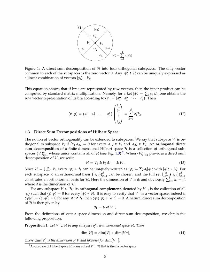
Figure 1: A direct sum decomposition of H into four orthogonal subspaces. The only vectorcommon to each of the subspaces is the zero vector 0. Any |ψy P H can be uniquely expressed asa linear combination of vectors |φiy P Vi.
This equation shows that if bras are represented by row vectors, then the inner product can becomputed by standard matrix multiplication. Namely, for a ket |ψy =
°k ak|ky, one obtains the
row vector representation of its bra according to xψ| .=(a�1 a�2 � � � a�d
). Then
xψ|ϕy = (a�1 a�2 � � � a�d)
b1b2...
bd
=d
k=1
a�k bk. (12)
1.3 Direct Sum Decompositions of Hilbert Space
The notion of vector orthogonality can be extended to subspaces. We say that subspace V1 is or-thogonal to subspace V2 if xα1|α2y = 0 for every |α1y P V1 and |α2y P V2. An orthogonal directsum decomposition of a finite-dimensional Hilbert space H is a collection of orthogonal sub-spaces tViun
i=1 whose union contains all of H (see Fig. 1.3) 2. When tViuni=1 provides a direct sum
decomposition of H, we writeH = V1 `V2 ` � � � `Vn. (13)
Since H =�n
i=1 Vi, every |ψy P H can be uniquely written as |ψy = °i ai|ϕiy with |ϕiy P Vi. Foreach subspace Vi an orthonormal basis t|ei,kyudi
k=1 can be chosen, and the full set�n
i=1t|ei,kyudik=1
constitutes an orthonormal basis for H. Here the dimension of Vi is di and obviously°t
i=1 di = d,where d is the dimension of H.
For any subspace V � H, its orthogonal complement, denoted by VK, is the collection of all|ϕy such that xψ|ϕy = 0 for every |ψy P H. It is easy to verify that VK is a vector space; indeed ifxψ|ϕy = xψ|ϕ1y = 0 for any |ψy P H, then xψ|(|ϕy+ |ϕ1y) = 0. A natural direct sum decompositionof H is then given by
H = V `VK.
From the definitions of vector space dimension and direct sum decomposition, we obtain thefollowing proposition.
Proposition 1. Let V � H be any subspace of a d-dimensional space H. Then
dim[H] = dim[V] + dim[VK], (14)
where dim[V] is the dimension of V and likewise for dim[VK].2A subspace of Hilbert space H is any subset V � H that is itself a vector space
5
2 Linear Operators
2.1 Outer Products, Adjoints, and Eigenvalues
For two Hilbert spaces H1 and H2, a linear operator R is simply a linear function that maps vectorsin H1 to H2. That is, for any |αy, |βy P H1 and any a, b P C, the operator R has action
R (a|αy+ b|βy) = aR|αy+ bR|βy P H2. (15)
We denote the set of all linear operators mapping H1 to H2 by L(H1,H2). For example, the vectorspace of bras acting H is precisely the set L(H, C). When H1 = H2 = H, we denote L(H1,H2)simply by L(H).
Equation (15) implies that every linear operator is defined by its action on a basis. Specificallyif H1 is a d1-dimensional space with computational basis t|iyud1
i=1, then an operator R P L(H1,H2)acts on this basis according to
R|iy =d2
j=1
Rji|jy for k = 1, � � � , d1,
where t|jyud2j=1 is the computational basis in H2. By contracting both the RHS and LHS with xj|, we
see thatRji = xj|R|iy. (16)
Bra-ket notation provides a convenient way to write any linear operator. With respect to basest|iyud1
i=1 for H1 and t|jyud2j=1 for H2, any linear operator R can be written as
R =d1
i=1
d2
j=1
Rji|jyxi|. (17)
When R acts on a state |ψy, the transformed state is
R|ψy = d1
i=1
d2
j=1
Rji|jyxi| |ψy = d1
i=1
d2
j=1
Rjixi|ψy|jy. (18)
In general, the “ket-bra” |βyxα| is called the outer product of kets |αy P H1 and |βy P H2. It is thelinear operator in L(H1,H2) that acts on an arbitrary ket |ψy by outputting the ket |βy multipliedby the bra-ket (i.e. the inner product) xα|ψy:
|ψy Ñ (|βyxα|) |ψy = xα|ψy|βy. (19)
Eqns. (16) and (17) show how a linear operator can be represented as a matrix. Using basest|iyud1
i=1 and t|jyud2j=1 for H1 and H2 respectively, an operator R can has the matrix representation
R .=
x1|R|1y x1|R|2y � � � x1|R|d1yx2|R|1y x2|R|2y � � � x2|R|d1y
... � � � ...xd2|R|1y xd2|R|2y � � � xd2|R|d1y
. (20)
6
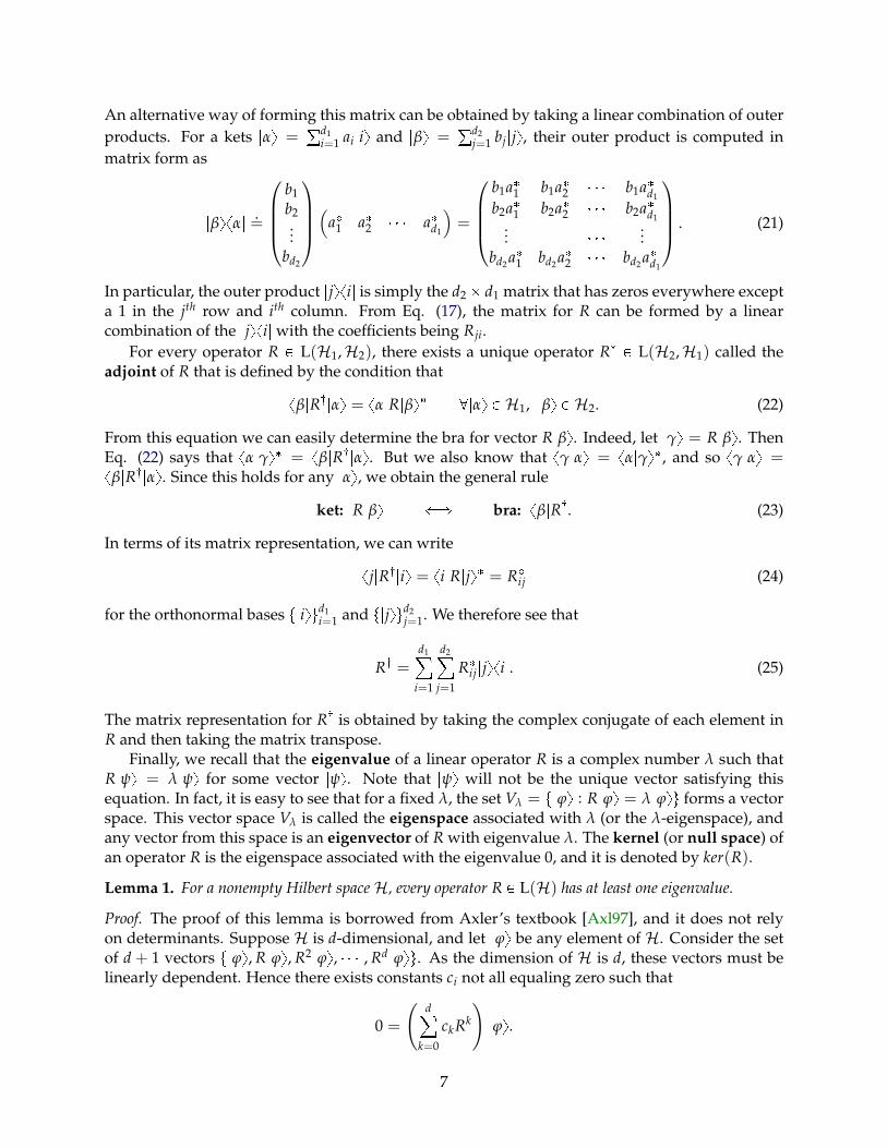
An alternative way of forming this matrix can be obtained by taking a linear combination of outerproducts. For a kets |αy =
°d1i=1 ai|iy and |βy =
°d2j=1 bj|jy, their outer product is computed in
matrix form as
|βyxα| .=
b1b2...
bd2
(a�1 a�2 � � � a�d1
)=
b1a�1 b1a�2 � � � b1a�d1
b2a�1 b2a�2 � � � b2a�d1... � � � ...
bd2 a�1 bd2 a�2 � � � bd2 a�d1
. (21)
In particular, the outer product |jyxi| is simply the d2 � d1 matrix that has zeros everywhere excepta 1 in the jth row and ith column. From Eq. (17), the matrix for R can be formed by a linearcombination of the |jyxi| with the coefficients being Rji.
For every operator R P L(H1,H2), there exists a unique operator R: P L(H2,H1) called theadjoint of R that is defined by the condition that
xβ|R:|αy = xα|R|βy� @|αy P H1, |βy P H2. (22)
From this equation we can easily determine the bra for vector R|βy. Indeed, let |γy = R|βy. ThenEq. (22) says that xα|γy� = xβ|R:|αy. But we also know that xγ|αy = xα|γy�, and so xγ|αy =xβ|R:|αy. Since this holds for any |αy, we obtain the general rule
ket: R|βy ðñ bra: xβ|R:. (23)
In terms of its matrix representation, we can write
xj|R:|iy = xi|R|jy� = R�ij (24)
for the orthonormal bases t|iyud1i=1 and t|jyud2
j=1. We therefore see that
R: =d1
i=1
d2
j=1
R�ij|jyxi|. (25)
The matrix representation for R: is obtained by taking the complex conjugate of each element inR and then taking the matrix transpose.
Finally, we recall that the eigenvalue of a linear operator R is a complex number λ such thatR|ψy = λ|ψy for some vector |ψy. Note that |ψy will not be the unique vector satisfying thisequation. In fact, it is easy to see that for a fixed λ, the set Vλ = t|ϕy : R|ϕy = λ|ϕyu forms a vectorspace. This vector space Vλ is called the eigenspace associated with λ (or the λ-eigenspace), andany vector from this space is an eigenvector of R with eigenvalue λ. The kernel (or null space) ofan operator R is the eigenspace associated with the eigenvalue 0, and it is denoted by ker(R).
Lemma 1. For a nonempty Hilbert space H, every operator R P L(H) has at least one eigenvalue.
Proof. The proof of this lemma is borrowed from Axler’s textbook [Axl97], and it does not relyon determinants. Suppose H is d-dimensional, and let |ϕy be any element of H. Consider the setof d + 1 vectors t|ϕy, R|ϕy, R2|ϕy, � � � , Rd|ϕyu. As the dimension of H is d, these vectors must belinearly dependent. Hence there exists constants ci not all equaling zero such that
0 =
(d
k=0
ckRk
)|ϕy.
7

Now consider the polynomial p(z) =°d
k=0 ckzk for z P C. If instead of a complex number zwe substitute the operator R and multiply additive constants by the identity, then we obtainp(R) :=
°dk=0 ckRk, which is precisely the term in parentheses in the above equation. The fun-
damental theorem of algebra says that every degree d polynomial has d roots r1, r2, � � � , rd (in-cluding multiplicities), and so r(z) can be factored as p(z) = c
±dk=1(z� rk). Applying the same
factorization to p(R), we obtain
0 = p(R)|ϕy = cd¹
k=1
(R� rkI)|ϕy. (26)
This implies that there must exist some rk such that 0 = (R� rkI)|ϕky.We finally describe an important relationship between the kernel of R and its range. The range
(or image) of a linear operator R P L(H1,H2) is the vector space defined by
Rng(R) ="|ϕy P H2
���� |ϕy = R|ψy for some |ψy P H1
*.
The image of an operator is itself a vector space, a fact that can be easily verified. The dimension ofRng(R) is called the rank of R (denoted by rk(R)), and the following fundamental theorem relatesrk(R) and dim[ker(R)].
Theorem 1 (Rank-Nullity Theorem). For any operator R P L(H1,H2),
dim[H1] = rk(R) + dim[ker(R)]. (27)
Proof. By Prop. 1 we must show that rk(R) = dim[ker(R)K]. Expand R in the computational basisas
R =d1
i=1
d2
j=1
Rji|jyxi| =d2
j=1
|jyxφj| where xφj| =d1
i=1
Rjixi|.
From this we see that |ψy P ker(R) iff xφj|ψy = 0 for all j. In other words, t|φjyud1j=1 belong to
ker(R)K. Let us take t|εiyuri=1 as an orthonormal basis for ker(R)K so that we can write |φjy =°r
k=1 cjk|εky for every |φjy. Then
R =d2
j=1
|jyxφj| =d2
j=1
r
k=1
c�jk|jyxεk| =r
k=1
|νkyxεk|, (28)
where |νky =°d2
j=1 c�jk|jy. The t|νkyurk=1 must be linearly independent. Indeed, suppose that°
k=1 ak|νky = 0 for ak not all zero. Then |ψy =°r
i=1 a�i |εiy satisfies R|ψy = 0, which is impos-sible since all the |εiy belong to ker(R)K. Hence, the t|νkyur
k=1 are linearly independent, and theyclearly span Rng(R). This proves that r = dim[ker(R)K] = dim[Rng(R)].
Typically, the rank of an operator R is defined as the dimension of the column space (or rowspace) when R is represented as a matrix. Eq. (28) shows that this is equivalent to the definitiongiven here of rk(R) = dim[Rng(R)]. Indeed, the t|νkyur
k=1 are precisely the column vectors whenexpressing R in an t|εkyuk basis of H1.
8
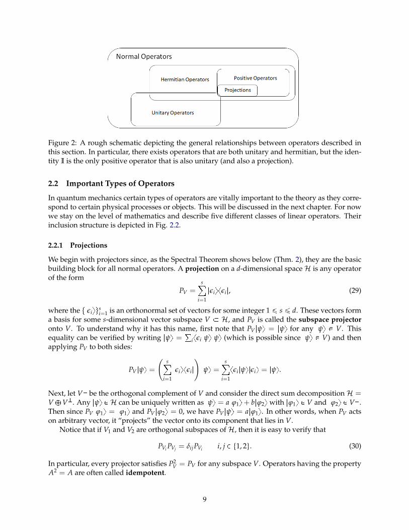
Figure 2: A rough schematic depicting the general relationships between operators described inthis section. In particular, there exists operators that are both unitary and hermitian, but the iden-tity I is the only positive operator that is also unitary (and also a projection).
2.2 Important Types of Operators
In quantum mechanics certain types of operators are vitally important to the theory as they corre-spond to certain physical processes or objects. This will be discussed in the next chapter. For nowwe stay on the level of mathematics and describe five different classes of linear operators. Theirinclusion structure is depicted in Fig. 2.2.
2.2.1 Projections
We begin with projectors since, as the Spectral Theorem shows below (Thm. 2), they are the basicbuilding block for all normal operators. A projection on a d-dimensional space H is any operatorof the form
PV =s
i=1
|εiyxεi|, (29)
where the t|εiyusi=1 is an orthonormal set of vectors for some integer 1 ¤ s ¤ d. These vectors form
a basis for some s-dimensional vector subspace V � H, and PV is called the subspace projectoronto V. To understand why it has this name, first note that PV |ψy = |ψy for any |ψy P V. Thisequality can be verified by writing |ψy = °ixεi|ψy|ψy (which is possible since |ψy P V) and thenapplying PV to both sides:
PV |ψy =(
s
i=1
|εiyxεi|)|ψy =
s
i=1
xεi|ψy|εiy = |ψy.
Next, let VK be the orthogonal complement of V and consider the direct sum decomposition H =V `VK. Any |ψy P H can be uniquely written as |ψy = a|ϕ1y+ b|ϕ2y with |ϕ1y P V and |ϕ2y P VK.Then since PV |ϕ1y = |ϕ1y and PV |ϕ2y = 0, we have PV |ψy = a|ϕ1y. In other words, when PV actson arbitrary vector, it “projects” the vector onto its component that lies in V.
Notice that if V1 and V2 are orthogonal subspaces of H, then it is easy to verify that
PVi PVj = δijPVi i, j P t1, 2u. (30)
In particular, every projector satisfies P2V = PV for any subspace V. Operators having the property
A2 = A are often called idempotent.
9
For s ¡ 1, there are an infinite number of orthonormal bases for a given s-dimensional sub-space V, and each of these provides a different way to represent the subspace projector. In otherwords, if t|εiyus
i=1 and t|δiyusi=1 are both orthonormal bases for V, then
s
i=1
|εiyxεi| =s
i=1
|δiyxδi|.
An extreme case is when V is the entire vector space H. In this case, the subspace projector issimply the identity operator I, i.e. the unique operator in L(H) satisfying I|ψy = |ψy for all|ψy P H. Then if t|εiyud
i=1 is any orthonormal basis for H, we can express the identity as
I =d
i=1
|εiyxεi|
Throughout this course we will work heavily with the eigenspaces of various operators. Foran operator R with eigenvalue λ, we define its λ-eigenprojector to be the projector Pλ that projectsonto the λ-eigenspace Vλ.
2.2.2 Normal Operators
An operator N P L(H) is called normal if NN: = N:N. Note, each normal operator is representedby a square matrix since it maps a given vector space H onto itself. In general, every normaloperator has very nice mathematical properties, two of which are the following.
Proposition 2. If N P L(H) is normal with eigenvalue λ and eigenspace Vλ, then λ� is an eigenvalue N:
with eigenspace Vλ.
Proof. First, let |ψy be any element in Vλ. By assumption we have that (N � λI)|ψy = 0. It is easyto see that if N is normal, then so is N � λI. Therefore,
0 = xψ|(N � λI):(N � λI)|ψy= xψ|(N � λI)(N � λI):|ψy. (31)
The last line implies that (N: � λ�I)|ψy = 0, which is what we set out to prove.
Proposition 3. If N P L(H) is normal with distinct eigenvalues λ1 and λ2, then the associated eigenspacesVλ1 and Vλ2 are orthogonal. Furthermore, H =
�λi
Vλi , where the union is taken over all distinct eigen-values of N.
Proof. Let |ψ1y P Vλ1 and |ψ2y P Vλ2 be arbitrary. Then (i) N|ψ1y = λ1|ψ1y, and (ii) N:|ψ2y = λ�2 |ψ2y.
Hence
xψ2|N|ψ1y = xψ2| (N|ψ1y) = λ1xψ2|ψ1y= (xψ2|N) |ψ1y = λ2xψ2|ψ1y, (32)
where the second line follows from (ii). Subtracting these gives xψ2|ψ1y = 0.To prove the second claim of the proposition let V =
�λi
Vλi . We want to show that VK = H.To this end, let pN be the operator N with domain restricted to VK; that is, pN : VK Ñ H with actiondefined by pN|βy = N|βy for all |βy P VK. Notice that for any |αy P V and |βy P VK we have
xα| pN|βy = xα|N|βy = xβ|N:|αy� = 0,
10
where we have used Prop. 2 to conclude that N:|αy P V. This shows that pN maps VK onto itself;i.e. pN P L(VK). Therefore, we can use Lem. 1 which says that if VK is nonempty, then pN has atleast one eigenvalue and eigenvector. But this would be a contradiction since any eigenvector ofpN is also an eigenvector N, and all eigenspaces of N are contained in V. Hence VK must by theempty set.
Proposition 3 shows that every normal operator N P L(H) is uniquely associated with a directsum decomposition
H = Vλ1 `Vλ2 ` � � � `Vλn (33)
where the Vλi are the eigenspaces of N. This directly leads to the spectral decomposition of N,which is one of the most important mathematical theorems in quantum mechanics.
Theorem 2 (Spectral Decomposition). Every normal operator N P L(H) can be uniquely written as
N =n
i=1
λiPλi , (34)
where the tλiuni=1 are the distinct eigenvalues of N and the tPλiun
i=1 are the corresponding eigenspaceprojectors.
Proof. By the direct sum decomposition of Eq. (33), any vector |ψy P H can be written as |ψy =°ni=1 |αiy with |αiy P Vλi . Thus,
(N �n
i=1
λiPλi)|ψy = Nn
i=1
|αiy �n
i=1
λiPλi
n
j=1
|αjy =n
i=1
λi|αiy �n
i=1
λi|αiy = 0.
Since this holds for all |ψy P H, we must have (N �°ni=1 λiPλi) = 0, or N =
°ni=1 λiPλi .
If a normal operator has a zero eigenvalue, then the associated eigenspace is ker(N). The vectorspace
supp(N) := ker(N)K =¤
λk �=0
Vλk (35)
is called the support of N, and it is denoted by supp(N). From the spectral decomposition, wecan immediately see that the support of N is equivalent to its range; i.e. supp(N) = rng(N).
Since every projector is a normal operator, it also has a spectral decomposition. In fact, this isprecisely what is given in Eq. (29). Then if t|λi,jyudi
j=1 is an orthonormal basis for the eigenspaceVλi of a normal operator N, we can write the spectral decomposition of N as
N =n
i=1
λiPλi =n
i=1
λi
di
j=1
|λi,jyxλi,j| =n
i=1
di
j=1
λi|λi,jyxλi,j|. (36)
Customarily, we combine the two sums over (i, j) into a single sum where the same eigenvalueis counted multiple times. More precisely, the eigenvalue λi is counted dim[Vλi ] times. Since°n
i=1 di = d = dim[H] we can write
N =d
k=1
λk|λkyxλk|. (37)
As a matter of convention, whenever the λk are enumerated from k = 1, � � � , d we will assume thatthe set tλkud
k=1 may contain repeated eigenvalues. The full collection t|λkyudk=1 spans all of H, and
it is sometimes called a complete eigenbasis.
11
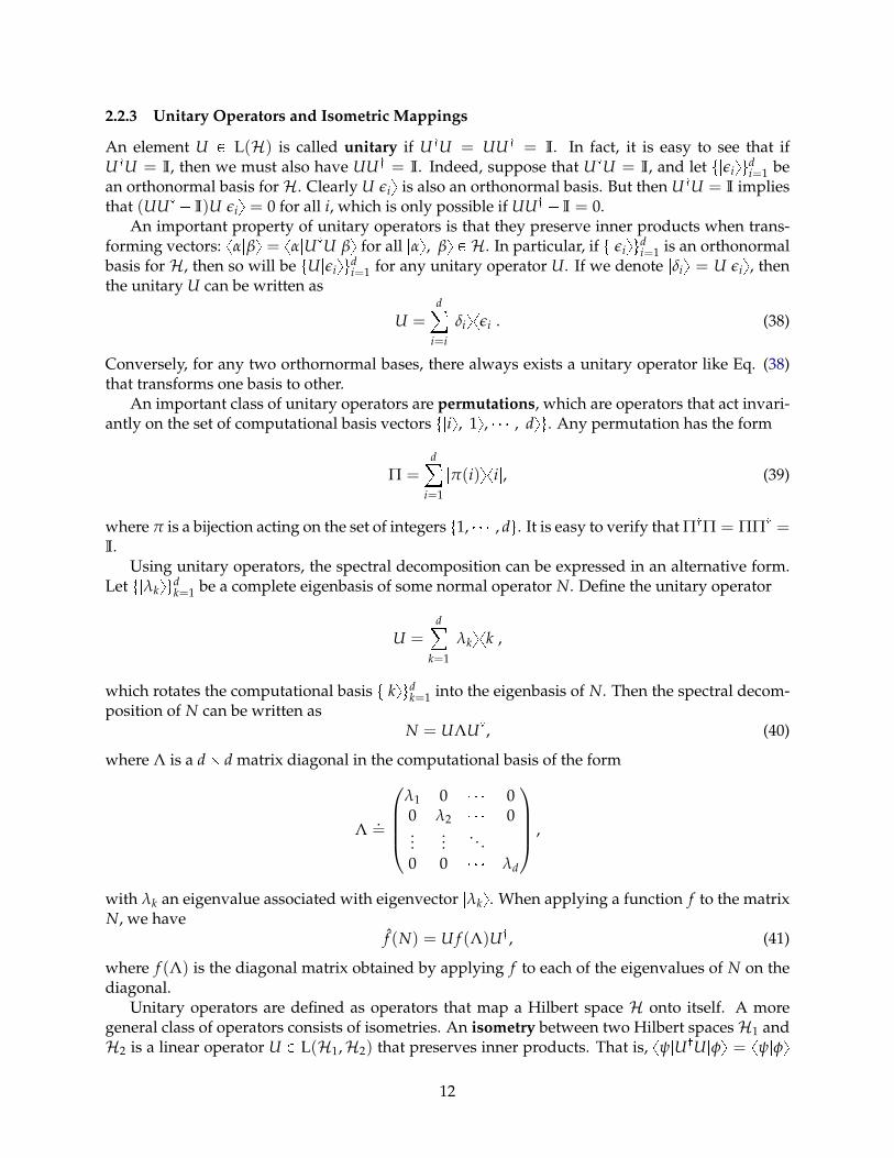
2.2.3 Unitary Operators and Isometric Mappings
An element U P L(H) is called unitary if U:U = UU: = I. In fact, it is easy to see that ifU:U = I, then we must also have UU: = I. Indeed, suppose that U:U = I, and let t|εiyud
i=1 bean orthonormal basis for H. Clearly U|εiy is also an orthonormal basis. But then U:U = I impliesthat (UU: � I)U|εiy = 0 for all i, which is only possible if UU: � I = 0.
An important property of unitary operators is that they preserve inner products when trans-forming vectors: xα|βy = xα|U:U|βy for all |αy, |βy P H. In particular, if t|εiyud
i=1 is an orthonormalbasis for H, then so will be tU|εiyud
i=1 for any unitary operator U. If we denote |δiy = U|εiy, thenthe unitary U can be written as
U =d
i=i
|δiyxεi|. (38)
Conversely, for any two orthornormal bases, there always exists a unitary operator like Eq. (38)that transforms one basis to other.
An important class of unitary operators are permutations, which are operators that act invari-antly on the set of computational basis vectors t|iy, |1y, � � � , |dyu. Any permutation has the form
Π =d
i=1
|π(i)yxi|, (39)
where π is a bijection acting on the set of integers t1, � � � , du. It is easy to verify that Π:Π = ΠΠ: =I.
Using unitary operators, the spectral decomposition can be expressed in an alternative form.Let t|λkyud
k=1 be a complete eigenbasis of some normal operator N. Define the unitary operator
U =d
k=1
|λkyxk|,
which rotates the computational basis t|kyudk=1 into the eigenbasis of N. Then the spectral decom-
position of N can be written asN = UΛU:, (40)
where Λ is a d� d matrix diagonal in the computational basis of the form
Λ .=
λ1 0 � � � 00 λ2 � � � 0...
.... . .
0 0 � � � λd
,
with λk an eigenvalue associated with eigenvector |λky. When applying a function f to the matrixN, we have
f (N) = U f (Λ)U:, (41)
where f (Λ) is the diagonal matrix obtained by applying f to each of the eigenvalues of N on thediagonal.
Unitary operators are defined as operators that map a Hilbert space H onto itself. A moregeneral class of operators consists of isometries. An isometry between two Hilbert spaces H1 andH2 is a linear operator U P L(H1,H2) that preserves inner products. That is, xψ|U:U|φy = xψ|φy
12
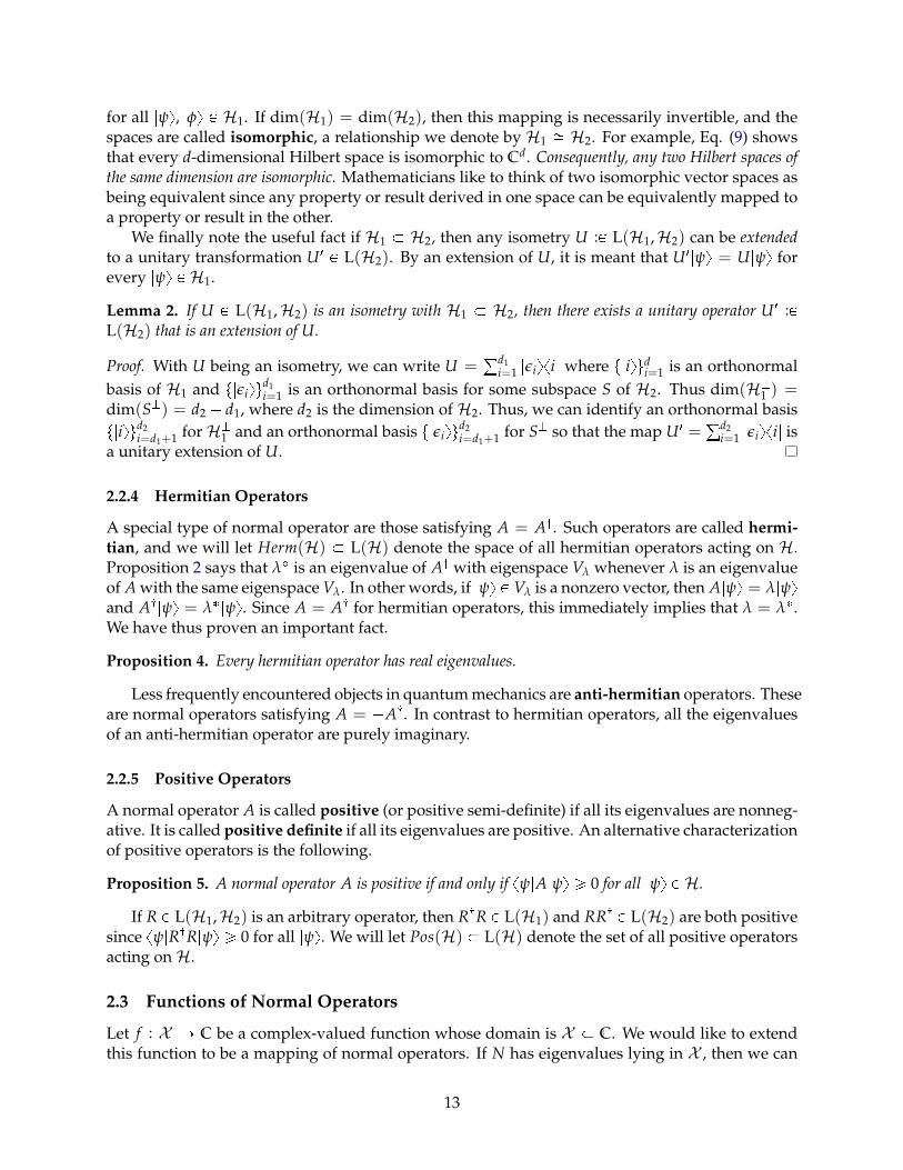
for all |ψy, |φy P H1. If dim(H1) = dim(H2), then this mapping is necessarily invertible, and thespaces are called isomorphic, a relationship we denote by H1 � H2. For example, Eq. (9) showsthat every d-dimensional Hilbert space is isomorphic to Cd. Consequently, any two Hilbert spaces ofthe same dimension are isomorphic. Mathematicians like to think of two isomorphic vector spaces asbeing equivalent since any property or result derived in one space can be equivalently mapped toa property or result in the other.
We finally note the useful fact if H1 � H2, then any isometry U :P L(H1,H2) can be extendedto a unitary transformation U1 P L(H2). By an extension of U, it is meant that U1|ψy = U|ψy forevery |ψy P H1.
Lemma 2. If U P L(H1,H2) is an isometry with H1 � H2, then there exists a unitary operator U1 :PL(H2) that is an extension of U.
Proof. With U being an isometry, we can write U =°d1
i=1 |εiyxi| where t|iyudi=1 is an orthonormal
basis of H1 and t|εiyud1i=1 is an orthonormal basis for some subspace S of H2. Thus dim(HK
1 ) =dim(SK) = d2 � d1, where d2 is the dimension of H2. Thus, we can identify an orthonormal basist|iyud2
i=d1+1 for HK1 and an orthonormal basis t|εiyud2
i=d1+1 for SK so that the map U1 =°d2
i=1 |εiyxi| isa unitary extension of U.
2.2.4 Hermitian Operators
A special type of normal operator are those satisfying A = A:. Such operators are called hermi-tian, and we will let Herm(H) � L(H) denote the space of all hermitian operators acting on H.Proposition 2 says that λ� is an eigenvalue of A: with eigenspace Vλ whenever λ is an eigenvalueof A with the same eigenspace Vλ. In other words, if |ψy P Vλ is a nonzero vector, then A|ψy = λ|ψyand A:|ψy = λ�|ψy. Since A = A: for hermitian operators, this immediately implies that λ = λ�.We have thus proven an important fact.
Proposition 4. Every hermitian operator has real eigenvalues.
Less frequently encountered objects in quantum mechanics are anti-hermitian operators. Theseare normal operators satisfying A = �A:. In contrast to hermitian operators, all the eigenvaluesof an anti-hermitian operator are purely imaginary.
2.2.5 Positive Operators
A normal operator A is called positive (or positive semi-definite) if all its eigenvalues are nonneg-ative. It is called positive definite if all its eigenvalues are positive. An alternative characterizationof positive operators is the following.
Proposition 5. A normal operator A is positive if and only if xψ|A|ψy ¥ 0 for all |ψy P H.
If R P L(H1,H2) is an arbitrary operator, then R:R P L(H1) and RR: P L(H2) are both positivesince xψ|R:R|ψy ¥ 0 for all |ψy. We will let Pos(H) � L(H) denote the set of all positive operatorsacting on H.
2.3 Functions of Normal Operators
Let f : X Ñ C be a complex-valued function whose domain is X � C. We would like to extendthis function to be a mapping of normal operators. If N has eigenvalues lying in X , then we can
13
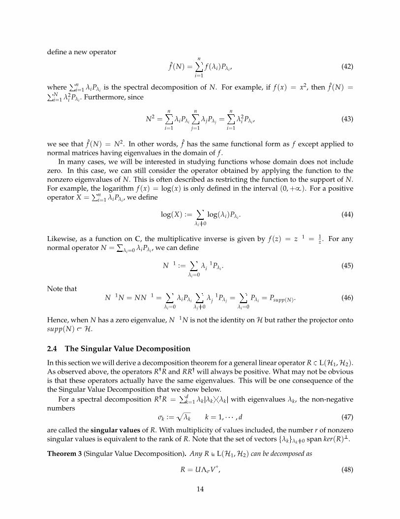
define a new operator
f (N) =n
i=1
f (λi)Pλi , (42)
where°n
i=1 λiPλi is the spectral decomposition of N. For example, if f (x) = x2, then f (N) =°Ni=1 λ2
i Pλi . Furthermore, since
N2 =n
i=1
λiPλi
n
j=1
λjPλj =n
i=1
λ2i Pλi , (43)
we see that f (N) = N2. In other words, f has the same functional form as f except applied tonormal matrices having eigenvalues in the domain of f .
In many cases, we will be interested in studying functions whose domain does not includezero. In this case, we can still consider the operator obtained by applying the function to thenonzero eigenvalues of N. This is often described as restricting the function to the support of N.For example, the logarithm f (x) = log(x) is only defined in the interval (0,+8). For a positiveoperator X =
°ni=1 λiPλi , we define
log(X) :=¸
λi �=0
log(λi)Pλi . (44)
Likewise, as a function on C, the multiplicative inverse is given by f (z) = z�1 = 1z . For any
normal operator N =°
λi �=0 λiPλi , we can define
N�1 :=¸
λi �=0
λ�1i Pλi . (45)
Note thatN�1N = NN�1 =
¸λi �=0
λiPλi
¸λj �=0
λ�1j Pλj =
¸λi �=0
Pλi = Psupp(N). (46)
Hence, when N has a zero eigenvalue, N�1N is not the identity on H but rather the projector ontosupp(N) � H.
2.4 The Singular Value Decomposition
In this section we will derive a decomposition theorem for a general linear operator R P L(H1,H2).As observed above, the operators R:R and RR: will always be positive. What may not be obviousis that these operators actually have the same eigenvalues. This will be one consequence of thethe Singular Value Decomposition that we show below.
For a spectral decomposition R:R =°d
k=1 λk|λkyxλk| with eigenvalues λk, the non-negativenumbers
σk :=a
λk k = 1, � � � , d (47)
are called the singular values of R. With multiplicity of values included, the number r of nonzerosingular values is equivalent to the rank of R. Note that the set of vectors tλkuλk �=0 span ker(R)K.
Theorem 3 (Singular Value Decomposition). Any R P L(H1,H2) can be decomposed as
R = UΛσV:, (48)
14
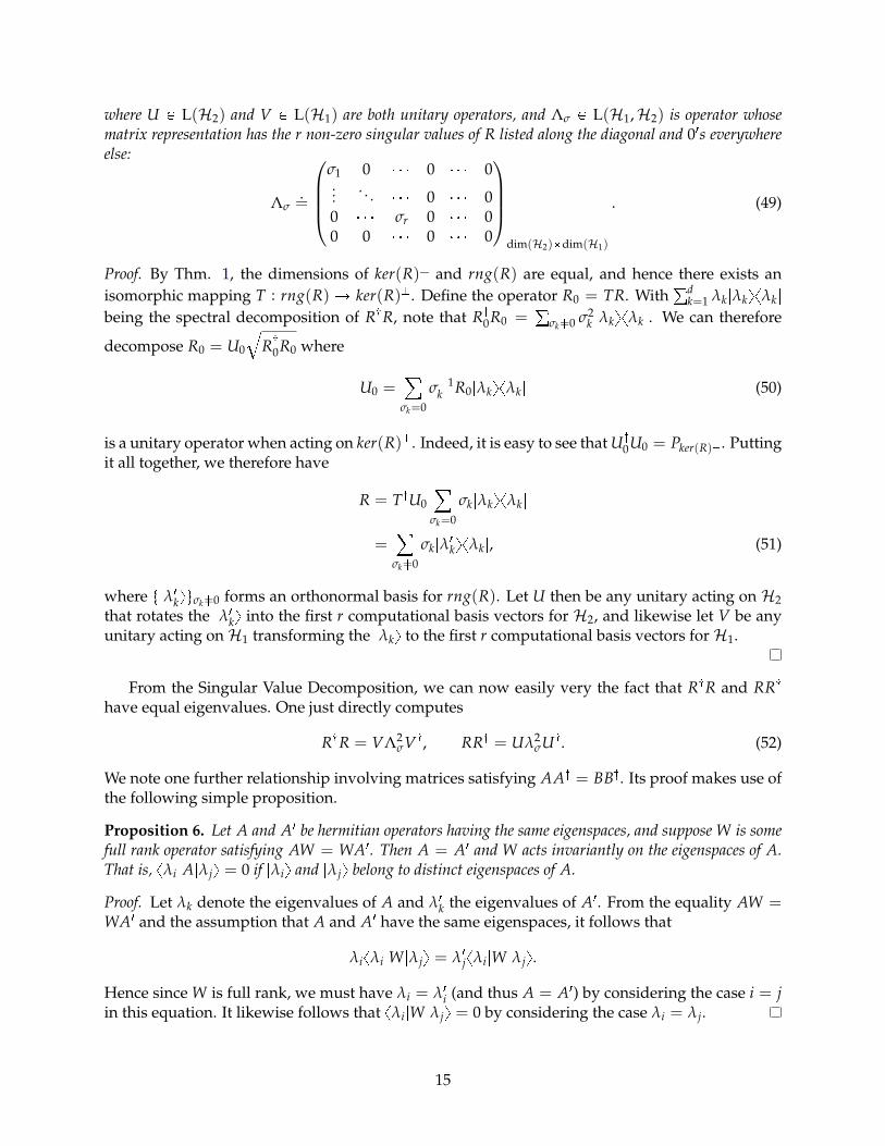
where U P L(H2) and V P L(H1) are both unitary operators, and Λσ P L(H1,H2) is operator whosematrix representation has the r non-zero singular values of R listed along the diagonal and 01s everywhereelse:
Λσ.=
σ1 0 � � � 0 � � � 0...
. . . � � � 0 � � � 00 � � � σr 0 � � � 00 0 � � � 0 � � � 0
dim(H2)�dim(H1)
. (49)
Proof. By Thm. 1, the dimensions of ker(R)K and rng(R) are equal, and hence there exists anisomorphic mapping T : rng(R) Ñ ker(R)K. Define the operator R0 = TR. With
°dk=1 λk|λkyxλk|
being the spectral decomposition of R:R, note that R:0R0 =
°σk �=0 σ2
k |λkyxλk|. We can therefore
decompose R0 = U0
bR:
0R0 where
U0 =¸
σk �=0
σ�1k R0|λkyxλk| (50)
is a unitary operator when acting on ker(R)K. Indeed, it is easy to see that U:0U0 = Pker(R)K . Putting
it all together, we therefore have
R = T:U0¸
σk �=0
σk|λkyxλk|
=¸
σk �=0
σk|λ1kyxλk|, (51)
where t|λ1kyuσk �=0 forms an orthonormal basis for rng(R). Let U then be any unitary acting on H2
that rotates the |λ1ky into the first r computational basis vectors for H2, and likewise let V be any
unitary acting on H1 transforming the |λky to the first r computational basis vectors for H1.
From the Singular Value Decomposition, we can now easily very the fact that R:R and RR:
have equal eigenvalues. One just directly computes
R:R = VΛ2σV:, RR: = Uλ2
σU:. (52)
We note one further relationship involving matrices satisfying AA: = BB:. Its proof makes use ofthe following simple proposition.
Proposition 6. Let A and A1 be hermitian operators having the same eigenspaces, and suppose W is somefull rank operator satisfying AW = WA1. Then A = A1 and W acts invariantly on the eigenspaces of A.That is, xλi|A|λjy = 0 if |λiy and |λjy belong to distinct eigenspaces of A.
Proof. Let λk denote the eigenvalues of A and λ1k the eigenvalues of A1. From the equality AW =
WA1 and the assumption that A and A1 have the same eigenspaces, it follows that
λixλi|W|λjy = λ1jxλi|W|λjy.
Hence since W is full rank, we must have λi = λ1i (and thus A = A1) by considering the case i = j
in this equation. It likewise follows that xλi|W|λjy = 0 by considering the case λi �= λj.
15
Lemma 3. For A P L(H1,H2) and B P L(H1,H3), if AA: = BB: then there exists a unitary U P L(H1)
such that A = UΛV:1 and B = UΛV:
2 are Singular Value Decompositions. A similar statement holdswhenever A:A = B:B for A P L(H2,H1) and B P L(H3,H1).
Proof. Let A = UAΛAV:A and B = UBΛBV:
B be Singular Value Decompositions of A. Decomposi-tion of A. Then the assumption AA: = BB: implies that Λ2
AW = WΛ2B, where W = U:
AUB. Fromthe previous proposition, we have that ΛA = ΛB =: Λ, and W applies block unitary transforma-tions on the blocks of Λ having the same singular value. Hence we have the commutation relationWΛ = WΛ(W:W) = ΛW, and consequently
B = UBΛV:B = UAWΛVB = UAΛ(WVB), (53)
which is what we want to prove.
3 Tensor Products
3.1 Tensor Product Spaces and Vectors
The tensor product is a construction that combines different Hilbert spaces to form one largeHilbert space. As we will see, tensor products are used to describe quantum systems composed ofmultiple subsystems. In anticipation of this application, we will henceforth label different Hilbertspaces by superscript capital letters (i.e. HA, HB, etc.) instead of by subscript numbers (i.e. H1,H2, etc.) The reason is that later we will associate Hilbert space HA with Alice, HB with Bob, etc.
If HA is a Hilbert space with computational basis t|iyAudAi=1 and HB is a Hilbert space with
computational basis t|iyBudBi=1, then their tensor product space is a Hilbert space HA bHB with
orthonormal basis given by t|iyAb |jyBudA,dBi=1,j=1, called a tensor product basis. Every vector |ψyAB P
HA bHB can be written as a linear combination of the basis vectors:
|ψyAB =dA
i=1
dB
j=1
cij|iyA b |jyB. (54)
In order to equip the tensor product space with more structure, we need a precise way to relateelements in HA and HB to elements in HA bHB. The tensor product is a map b : HA �HB ÑHA bHB that generates the tensor product vector |ψyA b |φyB P HA bHB for |ψyA P HA and|φyB P HB, such that
1. (c|ψyA)b |φyB = |ψyA b (c|φyB) = c(|ψyA b |φyB) @|ψyA P HA, |φyB P HB, c P C,
2. (|ψyA + |ωyA)b |φyB = |ψyA b |φyB + |ωyA b |φyB @|ψyA, |ωyA P HA, |φyB P HB,
3. |ψyA b (|φyB + |ωyB) = |ψyA b |φyB + |ψyA b |ωyB @|ψyA P HA, |φyB, |ωyB P HB.
These three properties are known as “bilinearity.” Hence, the tensor product is a bilinear mapfrom HA �HB to HA bHB.
One important consequence of bilinearity is that it allows us to form a tensor product basis forHA bHB using any pair of bases for HA and HB. Indeed suppose that t|i1yAudA
i=1 and t|j1yBudBj=1 are
16

arbitrary orthonormal bases for HA and HB respectively. Then we can write the computationalbasis vectors in these new bases by
|iyA =dA
j=1
aij|j1yA for i = 1, � � � , dA
|iyB =dB
j=1
bij|j1yB for i = 1, � � � , dB.
Substituting these into Eq. (54) and using bilinearity gives
|ψy =dA
i=1
dB
j=1
c1ij|i1yA b |j1yB, (55)
where c1ij =°dA
k=1°dB
l=1 aikbjlckl . Hence, t|i1yA b |j1yBudA,dBi=1,j=1 also provides a basis for HA bHB.
For notation simplicity, we will drop the superscript labels A and B on the kets when theassociated Hilbert spaces are clear. Also, the tensor product of two vectors |ψyb |φy is often writtenas |ψy|φy, or even just |ψφy.
It should be stressed that the the tensor product space HA bHB is much larger than the set oftensor product vectors. The latter is given by S = t|αyb |βy : |αy P HA, |βy P HBuwhile the formerconsists of all linear combinations of vectors in S . We have S � HA bHB, but S �= HA bHB sincenot every |ψy P HA bHB is a tensor product of two vectors. That is, |ψy �= |αy b |βy for most|ψy P HA bHB. We will later see that such vectors |ψy correspond to entangled states in quantumstates.
We next discuss the structure of linear operators acting on HA bHB. If A P L(HA,HA1
) andB P L(HB,HB1), then their tensor product Ab B is a linear operator HA bHB Ñ HA1 bHB1 withaction defined by
Ab B
¸i,j
cij|iy b |jy =
¸i,j
cij A|iy b B|jy. (56)
This action is linear such that if A, C P L(HA,HA1
) and B, D P L(HB,HB1), then Ab B + Cb D PL(HA bHB,HA1 bHB1) with action
(Ab B + CbD)|ψy = Ab B|ψy+ CbD|ψy (57)
for all |ψy P HA bHB. Furthermore, from Eq. (56) we see that the product of tensor productoperators satisfies
(Ab B)(CbD) = ACb BD. (58)
One important example of Eq. (56) is known as a partial contraction. If HA1
= C, then A PL(HA, C) is a bra acting on HA; i.e. A = xφ| for some |φy P HA. Letting HB = HB1 , then thepartial contraction of |φy on system A is the operator xφ|A b IB P L(HA bHB,HB) such that forany |ψyAB =
°i,j cij|iyA|jyB,
xφ|A b IB(|ψyAB) = xφ|A b IB
¸i,j
cij|iyA|jyB
=¸ij
cijxφ|iy|jyB. (59)
17
This is called a partial contraction since it is essentially contracting the two spaces HA and HB
down to the single space HB. Also note that if |γyAB =°
i,j ai,j|iy b |jy and |ωyAB =°
i,j bi,j|iy b |jyare two vectors in HA bHB, then their inner product represents a full contraction:
xγ|ωy =¸
i,j
a�i,jxi|A b xj|B(¸
k,l
bk,l|kyA b |lyB
)=¸
i,j,k,l
a�i,jbk,lxi|kyAxj|lyB =¸i,j
a�i,jbi,j. (60)
Next, recall that any operator A P L(HA,HA1
) and any operator B P L(HB,HB1) can be ex-pressed as
A =
dA1¸i=1
dA
k=1
aik|iyxk|, B =
dB1¸j=1
dB
l=1
bjl|jyxl|.
Likewise, any operator K P L(HA bHB,HA1 bHB1) can be expressed as
K =
dA1¸i=1
dA
k=1
dB1¸j=1
dB
l=1
cij,kl|iyxk| b |jyxl|. (61)
Analogous to the case of vectors in HA bHB, not every K P L(HA bHB,HA1 bHB1) is a tensorproduct of operators from L(HA,HA1
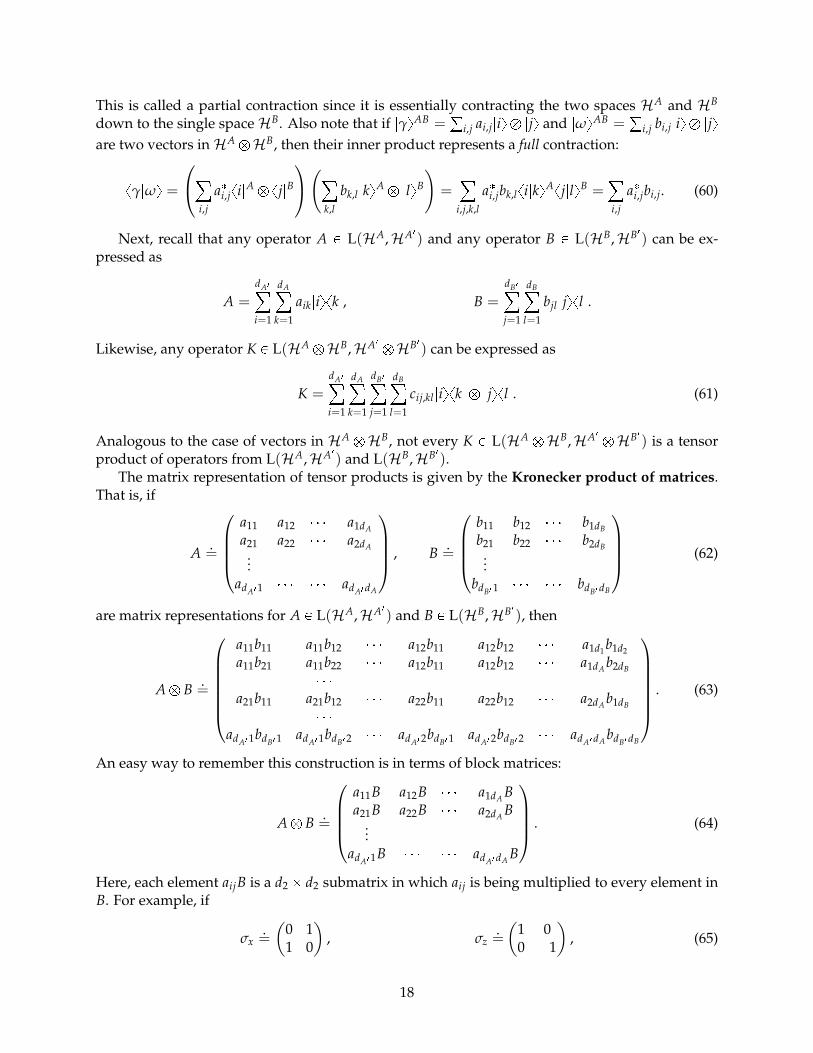
) and L(HB,HB1).The matrix representation of tensor products is given by the Kronecker product of matrices.
That is, if
A .=
a11 a12 � � � a1dA
a21 a22 � � � a2dA...
adA11 � � � � � � adA1dA
, B .=
b11 b12 � � � b1dB
b21 b22 � � � b2dB...
bdB11 � � � � � � bdB1dB
(62)
are matrix representations for A P L(HA,HA1
) and B P L(HB,HB1), then
Ab B .=
a11b11 a11b12 � � � a12b11 a12b12 � � � a1d1 b1d2
a11b21 a11b22 � � � a12b11 a12b12 � � � a1dA b2dB
� � �a21b11 a21b12 � � � a22b11 a22b12 � � � a2dA b1dB
� � �adA11bdB11 adA11bdB12 � � � adA12bdB11 adA12bdB12 � � � adA1dA bdB1dB
. (63)
An easy way to remember this construction is in terms of block matrices:
Ab B .=
a11B a12B � � � a1dA Ba21B a22B � � � a2dA B
...adA11B � � � � � � adA1dA B
. (64)
Here, each element aijB is a d2 � d2 submatrix in which aij is being multiplied to every element inB. For example, if
σx.=
(0 11 0
), σz
.=
(1 00 �1
), (65)
18
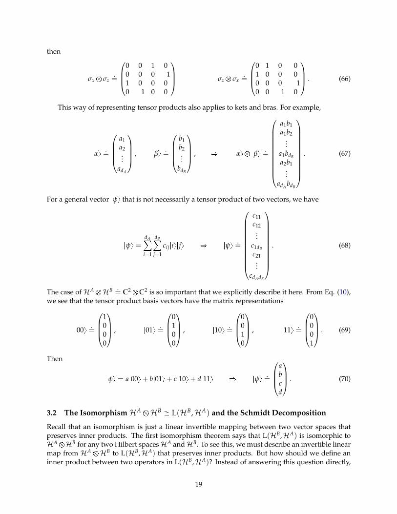
then
σx b σz.=
0 0 1 00 0 0 �11 0 0 00 �1 0 0
σz b σx.=
0 1 0 01 0 0 00 0 0 �10 0 �1 0
. (66)
This way of representing tensor products also applies to kets and bras. For example,
|αy .=
a1a2...
adA
, |βy .=
b1b2...
bdB
, ñ |αy b |βy .=
a1b1a1b2
...a1bdB
a2b1...
adA bdB
. (67)
For a general vector |ψy that is not necessarily a tensor product of two vectors, we have
|ψy =dA
i=1
dB
j=1
cij|iy|jy ñ |ψy .=
c11c12...
c1dB
c21...
cdAdB
. (68)
The case of HA bHB .= C2 bC2 is so important that we explicitly describe it here. From Eq. (10),
we see that the tensor product basis vectors have the matrix representations
|00y .=
1000
, |01y .=
0100
, |10y .=
0010
, |11y .=
0001
. (69)
Then
|ψy = a|00y+ b|01y+ c|10y+ d|11y ñ |ψy .=
abcd
. (70)
3.2 The Isomorphism HA bHB � L(HB,HA) and the Schmidt Decomposition
Recall that an isomorphism is just a linear invertible mapping between two vector spaces thatpreserves inner products. The first isomorphism theorem says that L(HB,HA) is isomorphic toHAbHB for any two Hilbert spaces HA and HB. To see this, we must describe an invertible linearmap from HA bHB to L(HB,HA) that preserves inner products. But how should we define aninner product between two operators in L(HB,HA)? Instead of answering this question directly,
19

let us first describe an invertible mapping from HA bHB to L(HB,HA), and then in the nextsection we will use this map to define an inner product on L(HB,HA) so that the two spacesbecome isomorphic.
Let t|iyudAi=1 be the computational basis specified for HA and t|jyudB
j=1 the computational basisfor HB. Then we introduce the following one-to-one association between elements in HA bHB
with elements in L(HB,HA):
|ψy =dA
i=1
dB
j=1
mij|iy|jy ØdA
i=1
dB
j=1
mij|iyxj| =: M|ψy. (71)
Using our established notation, we denote the equivalence between |ψy and M|ψy as |ψy .= M|ψy.
Thus, any vector |ψy in the tensor product space HA bHB can uniquely identified with a linear operatorM|ψy in L(HB,HA) and vice-versa.
In practice this equivalence is very easy to use since one just needs to remember the rule
|iy|jy Ø |iyxj|. (72)
However, there are a few words of caution here. First, this mapping is basis-dependent since itis defined in terms of the computational basis for HA and HB. For example, suppose we hadchosen some other bases t|i1yudA
i=1 and t|j1yudBj=1 and defined the mapping between HA bHB and
L(HA,HB) according to the rule |i1y|j1y Ø |i1yxj1|. Then we would end up associating a differentoperator with |ψy then we would under the original mapping |iy|jy Ø |iyxj|. The reason is that inthe |i1y|j1y basis, |ψywill have different components mij, and therefore it will be identified with theoperator
°dAi=1°dB
j=1 m1ij|iyxj| which is different than
°dAi=1°dB
j=1 mij|iyxj|. Typically the subscript |ψyon M|ψy will be dropped when the associated vector in HA bHB is clear.
Another potential source of confusion arises when comparing Eq. (71) to the conversion be-tween kets and bras. Let |αy = °dA
i=1 ai|iy and |βy = °dBj=1 bj|jy be any two vectors expanded in the
computational bases. Then according to the mapping of Eq. (71), the operator associated with thevector |αy|βy is
M|αy|βy =dA
i=1
dB
j=1
aibj|iyxj| �= |αyxβ|. (73)
The reason for this inequality is because the bra of |βy is given by xβ| = °dBj=1 b�j xj|. Hence if we
define the state |β�y :=°dB
j=1 b�j |jy, then we have
M|αy|βy = |αyxβ�|. (74)
The mapping of Eq. (71) can also be interpreted in operational terms. For a general d-dimensionalHilbert space H with computational basis t|jyudB
j=1, introduce the vector
|φ+d y =
d
j=1
|jjy (75)
which is an element of HbH. Here, HbH is representing two copies of the same Hilbert spaceH. Then for any |ψy P HA bHB with associated operator M = M|ψy P L(HB,HA), we can write
|ψy = Mb I|φ+dBy. (76)
20
This equality can be verified by noting the action of M|ψy on a basic vector |jy is given by
M|jyB =dA
i=1
mij|iyA. (77)
Then
|ψy =dA
i=1
dB
j=1
mij|iyA|jyB =dB
j=1
(dA
i=1
mij|iyA
)|jyB = Mb I|φ+
dBy. (78)
Thus, we can think of M|ψy as the operator that, when acting on the left side of |φ+dby generates the
state |ψy.It is also possible to switch the order of summations in Eq. (78). That is, we have
|ψy =dA
i=1
dB
j=1
mij|iyA|jyB =dA
i=1
|iyA
dB
j=1
mij|jyB
, (79)
The term in parentheses can be written as°dB
j=1 mij|jyB = MT|iyA, where MT :P L(HA,HB) is theoperator obtained by taking a transpose of M in the computational basis. Thus, we can write
|ψy = Ib MT|φ+dAy. (80)
Equations (76) and (80) are so useful in general that we state them in the following lemma, knownas the ricochet property.
Lemma 4 (Ricochet Property). An arbitrary A P L(HA,HB) satisfies
Ib A|φ+dAy = AT b I|φ+
dby, (81)
where AT P L(HB,HA) is the transpose of A taken in the computational bases, which are the same basesused to define |φ+
dAy and |φ+
dBy.
Our next task is to translate the Singular Value Decomposition of an operator in L(HA,H)) todecomposition of vectors in HA bHB. This is known as the Schmidt Decomposition, and it is oneof the most important tools in the study quantum entanglement.
Theorem 4 (Schmidt Decomposition). Every vector |ψy P HA bHB can be written as
|ψy =r
i=1
σi|αiy b |βiy, (82)
where t|αiyudAi=1 and t|βiyudB
i=1 are orthonormal bases called Schmidt bases for HA and HB respectively,the σi are positive numbers known as the Schmidt coefficients of |ψy, and r is known as the Schmidt rankof |ψy. Equivalently, the σi are the nonzero singular values of the operator M|ψy.
Proof. This proof of this is almost trivial given the ricochet property. Let M|ψy = UΛσV: be thesingular value decomposition of M|ψy. Then
|ψy = M|ψy b I|φ+dBy = UΛσV: b I|φ+
dBy =
dB
i=1
UΛσ|iy bV�|iy =r
i=1
σiU|iyA bV�|iyB
=r
i=1
σi|αiy b |βiy, (83)
where |αiy = U|iy and βi = V�|iy.
21
3.3 The Trace and Partial Trace
Let us now return to the question of establishing a true isomorphism between HA bHB andL(HB,HA). Given our one-to-one linear mapping in Eq. (71), what remains is to identify an in-ner product on L(HB,HA) that is preserved under this mapping. To be clear, we need a functionω : L(HB,HA)� L(HB,HA)Ñ C satisfying the axioms of the inner product and such that
ω
dA
i=1
dB
j=1
nij|iyxj|,dA
i=1
dB
j=1
mij|iyxj| = xφ|ψy =
dA
i=1
dB
j=1
n�ijmij, (84)
for any |ψy = °dAi=1°dB
j=1 mij|iy|jy and |φy = °dAi=1°dB
j=1 nij|iy|jy. This equality can be achieved usinga function known as the operator trace. For any X P L(H), its trace is defined as
Tr[X] =d
i=1
xεi|X|εiy, (85)
where t|εiyudi=1 is any orthonormal basis for H. Note that Tr : L(H)Ñ C is a linear mapping. Then
we can introduce an inner product on L(HB,HA), known as the Hilbert-Schmidt inner product,given by
ωHS(N, M) := Tr[N:M]. (86)
One can easily verify that the Hilbert-Schmidt inner product satisfies Eq. (84) thereby establishingthe isomorphism HA bHB � L(HB,HA).
The trace of an operator is used frequently in quantum mechanics. One important property ofthe trace is known as cyclicity. This says that
Tr[XYZ] = Tr[ZXY] = Tr[YZX]. (87)
This can be easily verified from the definition. Since°d
i=1 |εiyxεi| = I, we have, for instance,
Tr[XYZ] =d
i=1
xεi|XYZ|εiy =d
i,j,k=1
xεi|X|εjyxεj|Y|εkyxεk|Z|εiy
=d
i,j,k=1
xεk|Z|εiyxεi|X|εjyxεj|Y|εky = Tr[ZXY]. (88)
For a rank-one operator K = |ψyxφ|, its trace is easily found to be
Tr[|ψyxφ|] =d
i=1
xεi|ψyxφ|εiy =d
i=1
xφ|εiyxεi|φy = xψ|φy. (89)
On tensor product spaces, one can also define a partial trace. For any K P L(HA bHB) writtenas a sum of tensor products,
K =s
i=1
ci Ai b Bi (90)
with Ai P L(HA) and Bi P L(HB), the partial trace of K over HA is the operator in L(HB) given by
TrA[K] :=s
i=1
ci Tr[Ai]Bi. (91)
22
Likewise, the partial trace of HB over HB is
TrB[K] :=s
i=1
ci Tr[Bi]Ai. (92)
Linearity of the partial trace assures that TrA[K] and TrB[K] are well-defined.For rank-one positive operator K = |ψyxψ| P L(HA bHB), its partial traces are closely con-
nected to the Schmidt decomposition of |ψy P HA bHB and is operator representation M|ψy PL(HB,HA). Specifically, let |ψy = °r
i=1 σi|αiy b |βiy be a Schmidt decomposition of |ψy. Then
|ψyxψ| =r
i,j=1
σiσj|αiyxαj| b |βiyxβ j|. (93)
Since the Schmidt bases are orthonormal, we have
TrA[|ψyxψ|] =r
i,j=1
σiσj Tr[|αiyxαj|]|βiyxβ j| =r
i=1
σ2i |βiyxβi| = MT
|ψyM�|ψy. (94)
Likewise,
TrB[|ψyxψ|] =r
i=1
σ2i |αiyxαi| = M|ψyM:
|ψy. (95)
These relationships imply that if two vectors have the same Schmidt coefficients and Schmidtbases for either HA or HB, then the corresponding partial traces will be the same. Using Lem. 3we can show that the converse of this is also true.
Corollary 1. Suppose that |ψyAB and |φyAB are two vectors such that TrB |ψyxψ| = TrB |φyxφ|. Then|ψyAB and |φyAB have the same Schmidt coefficients, and there exists a common Schmidt basis t|αiyur
i=1 ofHA for both states. That is, there exists Schmidt decompositions
|ψy =r
i=1
σi|αiy b |βiy
|φy =r
i=1
σi|αiy b |β1iy. (96)
A similar statement holds when TrA |ψyxψ| = TrA |φyxφ|.Proof. This follows immediately from Lem. 3 and the ricochet property.
4 Exercises
Exercise 1
Suppose that H = C3 and let V be the one-dimensional subspace spanned by |ψy = ?1/3(|0y+
ei/3|1y � |2y). Provide an orthonormal basis for VK.
23

Exercise 2
Compute the eigenvalues and eigenvectors of the three matrices:
σx =
(0 11 0
), σy =
(0 �ii 0
)σz =
(1 00 �1
). (97)
Exercise 3
For a d-dimensional Hilbert space, compute the eigenvalues and dimensions of the associatedeigenspaces for the operators R1 = |βyxα| and R2 = I� |βyxα| when
(a) |αy = |βy;(b) |αy and |βy are orthogonal.
In both cases assume that |αy and |βy are normalized.
Exercise 4
Suppose that t|εiyusi=1 and t|δiyus
i=1 are both orthonormal bases for a subspace V P H. Showthat
s
i=1
|εiyxεi| =s
i=1
|δiyxδi| = PS.
Exercise 5
(a) Give an example of a normal operator that is not hermitian.
(b) Give an example of a unitary operator that is not hermitian.
(c) Give an example of a hermitian operator that is not positive.
Exercise 6
Prove Prop. 5. That is, show that a normal operator A is positive iff xψ|A|ψy ¥ 0 for all |ψy P H.
Exercise 7
Consider the operator R : R2 Ñ R2 given by
R = |0yx0|+ |1yx+|,
where |+y = ?1/2(|0y+ |1y). Find the singular value decomposition of R.
Exercise 8
For HA bHB .= C2 bC2, consider the operator Y P L(HA bHB) given by
Y = Ib σy � σy b I,
where σy is defined in Exercise 2.
24
(a) What is the matrix representation of Y in the computational basis?
(b) Compute Y|ψy with |ψy having the general form |ψy = a|00y+ b|01y+ c|10y+ d|11y.(c) Find a tensor product vector that is an eigenvector of Y (Hint: Use your answer from Exercise
2).
Exercise 9
For operators X and Y, compute their two partial traces TrA and TrB.
(a) X = |Φ+2 yxΦ+
2 |+ |0yx0| b |1yx1|, where |Φ+2 y =
?1/2(|00y+ |11y);
(b) Y = Fd, where F =°d
i,j=1 |ijyxji| is the d-dimensional SWAP operator.
Exercise 10
If X P L(HA bHB) is a positive operator, prove that both TrA[X] and TrB[X] are also positive.
References
[Axl97] S. Axler. Linear Algebra Done Right. Undergraduate Texts in Mathematics. Springer NewYork, 1997.
[Dir39] P. A. M. Dirac. A new notation for quantum mechanics. Mathematical Pro-ceedings of the Cambridge Philosophical Society, 35(3):416418, 1939. doi:10.1017/S0305004100021162.
25