linear algebra and its...
TRANSCRIPT

(FW I LEY
LINEAR ALGEBRAAND ITS APPLICATIONS Second Edition
aim
Pure and Applied Morhemotics:A Wiley-laterscienca Series of Texts, Monographs, and Tracts
Linear Algebra and ItsApplications

i;. 1 8 0 7:,1 9WILEY!zw 2 0 0 7'ererrfiti.h
THE WILEY BICENTENNIAL-KNOWLEDGE FOR GENERATIONS
(S ach generation has its unique needs and aspirations. When Charles Wiley firstopened his small printing shop in lower Manhattan in 1807. it was a generationof boundless potential searching for an identity. And we were there, helping todefine a new American literary tradition. Over half a century later, in the midstof the Second Industrial Revolution, it was a generation focused on building thefuture. Once again, we were there, supplying the critical scientific, technical, andengineering knowledge that helped frame the world. Throughout the 20thCentury, and into the new millennium, nations began to reach out beyond theirown borders and a new international community was born. Wiley was there,expanding its operations around the world to enable a global exchange of ideas,opinions, and know-how.
For 200 years, Wiley has been an integral part of each generation's journey,enabling the flow of information and understanding necessary to meet their needsand fulfill their aspirations. Today, bold new technologies are changing the waywe live and learn. Wiley will be there, providing you the must-have knowledgeyou need to imagine new worlds, new possibilities, and new opportunities.
Generations come and go, but you can always count on Wiley to provide you theknowledge you need, when and where you need it!
WILLIAM J. PESCE PETER BOOTH WILEYPRESIDENT AND CHIEF EXECLmvE OFFICER CHAIRMAN OF THE BOARD

Linear Algebra and ItsApplications
Second Edition
PETER D. LAX
New York UniversityCourant Institute of Mathematical SciencesNew York, NY
Ie[Nr[N N SAL
1 8 0 7
"*WILEY2007 !ale [Nv [NN111 LC
WILEY-LNTER.SCIENCEA JOHN WILEY & SONS, INC., PUBLICATION
Copyright Cl 2007 by John Wiley & Sons, Inc., Hoboken, New Jersey. All rights reserved.
Published simultaneously in Canada.
No pan of this publication may be reproduced, stored in a retrieval system or transmitted in any form orby any means, electronic, mechanical, photocopying, recording, scanning or otherwise, except aspermitted under Sections 107 or 108 of the 1976 United States Copyright Act, without either theprior written permission of the Publisher, or authorization through payment of the appropriatepercopy fee to the Copyright Clearance Center, 222 Rosewood Drive, Danvers, MA 01923,(978) 750-8400, fax (978) 750.4744. Requests to the Publisher for permission should be addressedto the Permissions Department, John Wiley & Sons, Inc., 605 Third Avenue, New York, NY 10158-0012,(212) 850-6011, fax (212) 850-6008, E-Mail: PERMREQ CO WILEY.COM.
For ordering and customer service, call 1-800-CALL-WILEY.
Wiley Bicentennial Logo: Richard J. Pacifico
Library of Congress Cataloging-in-Publication Data:
Lax, Peter D.Linear algebra and its applications / Peter D. Lax. - 2nd ed.
p. cm. - (Pure and applied mathematics. A Wiley-Interscience of texts, monographs and tracts)Previous ed.: Linear algebra. New York : Wiley, c1997.Includes bibliographical references and index.
ISBN 978-0-471-75156-4 (cloth)
1. Algebras, Linear. 1. Lax, Peter D. Linear algebra. 11. Title.
QAI84.2.L38 2008512'.5-dc22
2007023226
Printed in the United States of America1098765432I
Contents
PrefacePreface to the First Fditinn
1. FundamentalsLinear Space, IsomorphismSubspaceLinear DependenceBasis, DimensionQuotient Space
2. DualityLinear FunctionsDual of a Linear SpaceAnnihilatorCodimensionQuadrature Formula
3. Linear MappingsDomain and Target SpaceNullspace and RangeFundamental TheoremUnderdetermined Linear SystemsInterpolationDifference EquationsAlgebra of Linear MappingsDimension of Nullspace and RangeTranspositionSimilarityProjections
4. Matrices
Rows and ColumnsMatrix Multiplication
13
13
14
L
17
v

vi CONTENTS
TranspositionRankGaussian Elimination
5. Determinant and TraceOrdered SimplicesSigned Volume. DeterminantPermutation GroupFormula for DeterminantMultiplicative PropertyLaplace ExpansionC'ramer'c RuleTrace
6. Spectral TheoryIteration of Linear MapsEigenvalues. EigenvectorsFihonacci SequenceCharacteristic PolynomialTrace and Determinant RevisitedSpectral Mapping TheoremCayley-Hamilton TheoremGeneralized EigenvcctorsSpectral TheoremMinimal PolynomialWhen Are Two Matrices SimilarCommuting Maps
7- Euclidean StructureScalar Product. DistanceSchwarg InequalityOnhonormal BasisGram-SchmidtOrthogonal ComplementOrthogonal ProjectionAdjoinsOverdetermined SystemsIsometryThe Orthogonal GroupNorm of a Linear MapCompleteness Local CompactnessComplex Euclidean StructureSpectral RadiusHilhert-Schmidt NormCross Product
CONTENTS vii
8. Spectral Theory of Self-Adioint Mappings 101
Quadratic Forms 102
Law of Inertia AnSpectral Resolution 105
Commuting Maps 111
Anti-Self-Adjoint Maps 112
Normal Maps 112
Rayleigh Quotient 114
Minmax Principle 116
Norm and Eigenvalues 119
9. Calculus of Vector- and Matrix-Valued Functions mConvergence in Norm 121
Rules of Differentiation 1 11
Derivative of det A(r) 126
Matrix Exponential 128
Simple Eigenvalues 129
Multiple Eigenvalues 135
Rellich's Theorem 144
Avoidance of Crossing 140
10. Matrix Inequalities 143
Positive Self-Adjoint Matrices 143
Monotone Matrix Functions 1.5.1
Gram Matrices 1.52
Schur's Theorem 1.5.3
The Determinant of Positive Matrices 154
Integral Formula for Determinants 157
Eigenvalues 16()
Separation of Eigenvalues 161
Wielandt-Hoffman Theorem 1ASmallest and Largest Eigenvalue 166
Matrices with Positive Se]f-Adjoint Part 167
Polar Decomposition 169
Singular Values 170
Singular Value Decomposition 170
11. Kinematics and Dynamics 172
Axis and Angle of Rotation 172
Rigid Motion 173
Angular Velocity Vector 176
Fluid Flow 12Curl and Divergence 179
Small Vibrations ian
Conservation of Energy 182
Frequencies and Normal Modes 184
viii CONTENTS
12. Convexity 187
Convex Sets 187
Gauge Function 188
Hahn-Banach Theorem 191
Support Function 193
Caratheodorv's Theorem 195
Konig-Birkhoff Theorem 198
Helly's Theorem 199
13. The Duality Theorem 202
Farkas_Minkowski Theorem 203Duality Theorem 206
Economics Interpretation 208
Minmax Theorem 2151
14. Normed Linear Spaces 214
Norm 214
h Nouns 215Equivalence of Norms 217
Completeness 219
Local Compactness 219
Theorem of F. Ricsz 219
Dual Norm 222
Distance from Subspace 223
Normed Quotient Space 224
Complex Normed Spaces 226
Complex Hahn-Banach Theorem 226
Characterization of Euclidean Spaces 227
15. Linear Mappings Between Normed Linear Spaces 229
Norm of a Mapping 230
Norm of Transpose 231
Normed Algebra of Maps 232
invertible Maps 233
Spectral Radius 236
16. Positive Matrices 237
Perron's Theorem 237
Stochastic Matrices 240Frohenius' Theorem 243
17. How to Solve Systems of Linear Equations 246
History 246Condition Number 241E
Iterative Methods 24.8.
Steepest Descent 249
Chebychev Iteration 252

CONTENTS ix
Three-term Chebychev Iteration 255
Optimal Three-Teen Recursion Relation 256
Rate of Convergence 261
18. How to Calculate the Eigenvalues of Seif-Adjoint Matrices 262
QR Factorization 262
Using the QR Factorization to Solve Systems of Equations 263
The QR Algorithm for Finding Eigenvalues 263
Householder Reflection for OR Factorization 266
Tridiagonal Forni 267
Analogy of QR Algorithm and Toda Flow 269Mneer'x Theorem 223
More General Flows 276
19. Solutions 218
Bibliography 300
Appendix 1. Special Determinants 302
Appendix 2. The Pfaffian 305
Appendix 3. Symplectic Matrices 308
Appendix 4. Tensor Product 313
Appendix 5. Lattices 317
Appendix 6. Fast Matrix Multiplication 320
Appendix 7. Gershgorin's Theorem 323
Appendix 8. The Multiplicity of Eigenvalues 325
Appendix 9. The Fast Fourier Transform 328
Appendix 10. The Spectral Radius 334
Appendix 11. The Lorentz Group 342
Appendix 12. Compactness of the Unit Ball 352
Appendix 13. A Characterization of Commutators 355
Appendix 14. Liapunov's Theorem 357
Appendix 15. The Jordan Canonical Form 363
Appendix 16. Numerical Range 367
Index ,373

Preface
The outlook of this second edition is the same as that of the original: to present linearalgebra as the theory and practice of linear spaces and linear mappings. Where it aidsunderstanding and calculations, I don't hesitate to describe vectors as arrays ofnumbers and to describe mappings as matrices. Render onto Caesar the things whichare Caesar's.
If you can reduce a mathematical problem to a problem in linear algebra, you canmost likely solve it, provided that you know enough linear algebra. Therefore, athorough grounding in linear algebra is highly desirable. A sound undergraduateeducation should offer a second course on the subject, at the senior level. I wrote thisbook as a suitable text for such a course. The changes made in this second edition arepartly to make it more suitable as a text. Terse descriptions, especially in the earlychapters, were expanded, more problems were added, and a list of solutions toselected problems has been provided.
In addition, quite a bit of new material has been added, such as the compactnessof the unit ball as a criterion of finite dimensionality of a normed linear space. A newchapter discusses the QR algorithm for finding the eigenvalues of a self-adjointmatrix. The Householder algorithm for turning such matrices into tridiagonal form ispresented. I describe in some detail the beautiful observation of Deift, Nanda, andTomei of the analogy between the convergence of the QR algorithm and Moser'stheorem on the asymptotic behavior of the Toda flow as time tends to infinity.
Eight new appendices have been added to the first edition's original eight,including the Fast Fourier Transform, the spectral radius theorem, proved with thehelp of the Schur factorization of matrices, and an excursion into the theory ofmatrix-valued analytic functions. Appendix 11 describes the Lorentz group, 12 is aninteresting application of the compactness criterion for finite dimensionality, 13 is acharacterization of commutators, 14 presents a proof of Liapunov's stabilitycriterion, 15 presents the construction of the Jordan Canonical form of matrices, and16 describes Carl Pearcy's elegant proof of Halmos' conjecture about the numericalrange of matrices.
I conclude with a plea to include the simplest aspects of linear algebra in high-school teaching: vectors with two and three components, the scalar product, the
xi
Xii PREFACE
cross product, the description of rotations by matrices, and applications to geometry.Such modernization of the high-school curriculum is long overdue.
I acknowledge with pleasure much help I have received from Ray Michalek, aswell as useful conversations with Albert Novikoff and Charlie Peskin. I also wouldlike to thank Roger Horn, Beresford Parlett, and Jerry Kazdan for very usefulcomments, and Jeffrey Ryan for help in proofreading.
PETER D. LAX
New York. New York

Preface to the First Edition
This book is based on a lecture course designed for entering graduate students andgiven over a number of years at the Courant Institute of New York University. Thecourse is open also to qualified undergraduates and on occasion was attended bytalented high school students, among them Alan Edelman; I am proud to have beenthe first to teach him linear algebra. But, apart from special cases, the book, like thecourse, is for an audience that has some-not much-familiarity with linear algebra.
Fifty years ago, linear algebra was on its way out as a subject for research. Yetduring the past five decades there has been an unprecedented outburst of new ideasabout how to solve linear equations, carry out least square procedures, tacklesystems of linear inequalities, and find eigenvalues of matrices. This outburst camein response to the opportunity created by the availability of ever faster computerswith ever larger memories. Thus, linear algebra was thrust center stage in numericalmathematics. This had a profound effect, partly good, partly bad, on how the subjectis taught today.
The presentation of new numerical methods brought fresh and exciting material,as well as realistic new applications, to the classroom. Many students, after all, are ina linear algebra class only for the applications. On the other hand, bringingapplications and algorithms to the foreground has obscured the structure of linearalgebra-a trend I deplore; it does students a great disservice to exclude them fromthe paradise created by Emmy Noether and Emil Artin. One of the aims of this bookis to redress this imbalance.
My second aim in writing this book is to present a rich selection of analyticalresults and some of their applications: matrix inequalities, estimates for eigenvaluesand determinants, and so on. This beautiful aspect of linera algebra, so useful forworking analysts and physicists, is often neglected in texts.
I strove to choose proofs that are revealing, elegant, and short. When there aretwo different ways of viewing a problem, I like to present both.
The Contents describes what is in the book. Here I would like to explain mychoice of materials and their treatment. The first four chapters describe the abstracttheory of linear spaces and linear transformations. In the proofs I avoid eliminationof the unknowns one by one, but use the linear structure; I particularly exploit
xiii

AV PREFACE TO THE FIRST EDITION
quotient spaces as a counting device. This dry material is enlivened by somenontrivial applications to quadrature, to interpolation by polynomials, and to solvingthe Dirichlet problem for the discretized Laplace equation.
In Chapter 5, determinants are motivated geometrically as signed volumes ofordered simplices. The basic algebraic properties of determinants follow immediately.
Chapter 6 is devoted to the spectral theory of arbitrary square matrices withcomplex entries. The completeness of eigenvectors and generalized eigenvectors isproved without the characteristic equation, relying only on the divisibility theory ofthe algebra of polynomials. In the same spirit we show that two matrices A and B aresimilar if and only if (A - kI)t and (B - kl)"' have nullspaces of the samedimension for all complex k and all positive integer in. The proof of this propositionleads to the Jordan canonical form.
Euclidean structure appears for the first time in Chapter 7. It is used in Chapter 8to derive the spectral theory of selfadjoint matrices. We present two proofs, onebased on the spectral theory of general matrices, the other using the variationalcharacterization of eigenvectors and eigenvalues. Fischer's minmax theorem isexplained.
Chapter 9 deals with the calculus of vector- and matrix-valued functions of asingle variable, an important topic not usually discussed in the undergraduatecurriculum. The most important result is the continuous and differentiable characterof eigenvalues and normalized eigenvectors of differentiable matrix functions,provided that appropriate nondegeneracy conditions are satisfied. The fascinatingphenomenon of "avoided crossings" is briefly described and explained.
The first nine chapters, or certainly the first eight, constitute the core of linear algebra.The next eight chapters deal with special topics, to be taken up depending on the interestof the instructor and of the students. We shall comment on them very briefly.
Chapter 10 is a symphony of inequalities about matrices, their eigenvalues, andtheir determinants. Many of the proofs make use of calculus.
I included Chapter 11 to make up for the unfortunate disappearance of mechanicsfrom the curriculum and to show how matrices give an elegant description of motionin space. Angular velocity of a rigid body and divergence and curl of a vector field allappear naturally. The monotonic dependence of eigenvalues of symmetric matricesis used to show that the natural frequencies of a vibrating system increase if thesystem is stiffened and the masses are decreased.
Chapters 12, 13, and 14 are linked together by the notion of convexity. In Chapter12 we present the descriptions of convex sets in terms of gauge functions and supportfunctions. The workhorse of the subject, the hyperplane separation theorem, isproved by means of the Hahn-Banach procedure. Carathdodory's theorem onextreme points is proved and used to derive the Konig-Birkhoff theorem on doublystochastic matrices; Helly's theorem on the intersection of convex sets is stated andproved.
Chapter 13 is on linear inequalities; the Farkas-Minkowski theorem is derivedand used to prove the duality theorem, which then is applied in the usual fashion to amaximum-minimum problem in economics, and to the minmax theorem of vonNeumann about two-person zero-sum games.
PREFACE TO THE FIRST EDITION XV
Chapter 14 is on normed linear spaces; it is mostly standard fare except for a dualcharacterization of the distance of a point from a linear subspace. Linear mappingsof normed linear spaces are discussed in Chapter 15.
Chapter 16 presents Perron's beautiful theorem on matrices all of whose entriesare positive. The standard application to the asymptotics of Markov chains isdescribed. In conclusion, the theorem of Frobenius about the eigenvalues of matriceswith nonnegative entries is stated and proved.
The last chapter discusses various strategies for solving iteratively systems oflinear equations of the form Ax = b, A a self-adjoint, positive matrix. A variationalformula is derived and a steepest descent method is analyzed. We go on to presentseveral versions of iterations employing Chebyshev polynomials. Finally wedescribe the conjugate gradient method in terms of orthogonal polynomials.
It is with genuine regret that I omit a chapter on the numerical calculation ofeigenvalues of self-adjoint matrices. Astonishing connections have been discoveredrecently between this important subject and other seemingly unrelated topics.
Eight appendices describe material that does not quite fit into the flow of the text,but that is so striking or so important that it is worth bringing to the attention ofstudents. The topics I have chosen are special determinants that can be evaluatedexplicity, Pfaff's theorem, symplectic matrices, tensor product, lattices, Strassen'salgorithm for fast matrix multiplication, Gershgorin's theorem, and the multiplicityof eigenvalues. There are other equally attractive topics that could have been chosen:the Baker-Campbell-Hausdorff formula, the Kreiss matrix theorem, numericalrange, and the inversion of tridiagonal matrices.
Exercises are sprinkled throughout the text; a few of them are routine; mostrequire some thinking and a few of them require some computing.
My notation is neoclassical. I prefer to use four-letter Anglo-Saxon words like"into," "onto" and "1-to-1," rather than polysyllabic ones of Norman origin. Theend of a proof is marked by an open square.
The bibliography consists of the usual suspects and some recent texts; in addition,I have included Courant-Hilbert, Volume I, unchanged from the original Germanversion in 1924. Several generations of mathematicians and physicists, including theauthor, first learned linear algebra from Chapter 1 of this source.
I am grateful to my colleagues at the Courant Institute and to Myron Allen at theUniversity of Wyoming for reading and commenting on the manuscript and fortrying out parts of it on their classes. I am grateful to Connie Engle and Janice Wantfor their expert typing.
I have learned a great deal from Richard Bellman's outstanding book,Introduction to Matrix Analysis; its influence on the present volume is considerable.For this reason and to mark a friendship that began in 1945 and lasted until his deathin 1984, I dedicate this book to his memory.
PETER D. LAX
New York, New York


CHAPTER I
Fundamentals
This first chapter aims to introduce the notion of an abstract linear space to thosewho think of vectors as arrays of components. I want to point out that the class ofabstract linear spaces is no larger than the class of spaces whose elements are arrays.So what is gained by this abstraction?
First of all, the freedom to use a single symbol for an array; this way we can thinkof vectors as basic building blocks, unencumbered by components. The abstractview leads to simple, transparent proofs of results.
More to the point, the elements of many interesting vector spaces are notpresented in terms of components. For instance, take a linear ordinary differentialequation of degree n; the set of its solutions form a vector space of dimension n, yetthey are not presented as arrays.
Even if the elements of a vector space are presented as arrays of numbers, theelements of a subspace of it may not have a natural description as arrays. Take, forinstance, the subspace of all vectors whose components add up to zero.
Last but not least, the abstract view of vector spaces is indispensable for infinite-dimensional spaces; even though this text is strictly about finite-dimensional spaces,it is a good preparation for functional analysis.
Linear algebra abstracts the two basic operations with vectors: the addition ofvectors, and their multiplication by numbers (scalars). It is astonishing that on suchslender foundations an elaborate structure can be built, with romanesque, gothic, andbaroque aspects. It is even more astounding that linear algebra has not only the righttheorems but also the right language for many mathematical topics, includingapplications of mathematics.
A linear space X over afield K is a mathematical object in which two operationsare defined:
Addition, denoted by +, as in
(1)
Linear Algebra and Its Applications. Second Edition, by Peter D. LaxCopyright `'! 2007 John Wiley & Sons, Inc.
1
2 LINEAR ALGEBRA AND ITS APPLICATIONS
and assumed to be commutative:
x+y=y+x, (2)
and associative:
x+(y+z) = (x+y) +z,
and to form a group, with the neutral element denoted as 0:
x+0=x.
The inverse of addition is denoted by -:
x + (-x) =- x - x = 0.
EXERCISE I. Show that the zero of vector addition is unique.
(3)
(4)
(5)
The second operation is multiplication of elements of X by elements k of thefield K:
kx.
The result of this multiplication is a vector, that is, an element of X.Multiplication by elements of K is assumed to be associative:
k(ax) = (ka)x (6)
and distributive:
k(x + y) = kx + ky, (7)
as well as
(a + b)x = ax + bx. (8)
We assume that multiplication by the unit of K, denoted as 1, acts as the identity:
These are the axioms of linear algebra. We proceed to draw some deductions:Set b = 0 in (8); it follows from Exercise 1 that for all x
(9)
Ox=0. (10)
FUNDAMENTALS 3
Set a = 1, b = -1 in (8); using (9) and (10) we deduce that for all x
(-1)x = -x.
EXERCISE 2. Show that the vector with all components zero serves as the zeroelement of classical vector addition.
In this analytically oriented text the field K will be either the field Fl of realnumbers or the field C of complex numbers.
An interesting example of a linear space is the set of all functions x(t) that satisfythe differential equation
d2dt2x+x=0.
The sum of two solutions is again a solution, and so is the constant multiple of one.This shows that the set of solutions of this differential equation form a linear space.
Solutions of this equation describe the motion of a mass connected to a fixedpoint by a spring. Once the initial position x(0) = p and initial velocity drx(0) = vare given, the motion is completely determined for all t. So solutions can bedescribed by a pair of numbers (p, v).
The relation between the two descriptions is linear; that is, if (p, v) are the initialdata of a solution x(t), and (q, w) the initial data of another solution y(t), then theinitial data of the solution x(t) + y(t) are (p + q, v + w) = (p, v) + (q, w). Similarly,the initial data of the solution kx(t) are (kp, kv) = k(p, v).
This kind of relation has been abstracted into the notion of isomorphism.
Definition. A one-to-one correspondence between two linear spaces over thesame field that maps sums into sums and scalar multiples into scalar multiples iscalled an isomorphism.
Isomorphism is a basic notion in linear algebra. Isomorphic linear spaces areindistinguishable by means of operations available in linear spaces. Two linearspaces that are presented in very different ways can be, as we have seen, isomorphic.
E x a m p l e s o f Linear S p a c e s . (i) Set of all row vectors: (a, , ... , an), aj in K;addition, multiplication defined componentwise. This space is denoted as K".
(ii) Set of all real-valued functions f(x) defined on the real line, K = R.(iii) Set of all functions with values in K, defined on an arbitrary set S.(iv) Set of all polynomials of degree less than n with coefficients in K.
EXERCISE 3. Show that (i) and (iv) are isomorphic.
EXERCISE 4. Show that if S has n elements, (i) and (iii) are isomorphic.
4 LINEAR ALGEBRA AND ITS APPLICATIONS
EXERCISE 5. Show that when K = 08, (iv) is isomorphic with (iii) when Sconsists of n distinct points of R.
Definition. A subset Yof a linear space X is called a subspace if sums and scalarmultiples of elements of Y belong to Y.
Examples of Subspaces. (a) X as in Example (i), Y the set of vectors(0,a2-..,a,,-I,0) whose first and last component is zero.
(b) X as in Example (ii), Y the set of all periodic functions with period 7r.(c) X as in Example (iii), Y the set of constant functions on S.(d) X as in Example (iv), Y the set of all even polynomials.
Definition. The sum of two subsets Y and Z of a linear space X, denoted asY + Z, is the set of all vectors of form y + z, y in Y, z in Z.
EXERCISE 6. Prove that Y + Z is a linear subspace of X if Y and Z are.
Definition. The intersection of two subsets Yand Z of a linear space X, denotedas Y fl z, consists of all vectors x that belong to both Yand Z
EXERCISE 7. Prove that if Yand Z are linear subspaces of X, so is Y fl Z.
EXERCISE 8. Show that the set {0} consisting of the zero element of a linearspace X is a subspace of X. It is called the trivial subspace.
Definition. A linear combination of j vectors x, , .... x1 of a linear space is avector of the form
kixl k,,...,kJ E K.
EXERCISE 9. Show that the set of all linear combinations of x , , ... , xj is asubspace of X, and that it is the smallest subspace of X containing x, , ... , x1. This iscalled the subspace spanned by x, .... , xJ.
Definition. A set of vectors x, , ... , x, in X span the whole space X if everyx inX can be expressed as a linear combination of x,, ... ,x,,,.
Definition. The vectors x,,...,xj are called linearly dependent if there is anontrivial linear relation between them, that is, a relation of the form
=0,
where not all k, , ... , kJ are zero.
FUNDAMENTALS S
Definition. A set of vectors x1,. .. , xj that are not linearly dependent is calledlinearly independent.
EXERCISE 10. Show that if the vectors xi , ... , xj are linearly independent, thennone of the x; is the zero vector.
Lemma 1. Suppose that the vectors xi, ... , x,, span a linear space X and that thevectors y1, . . . , y, in X are linearly independent. Then
j < n.
Proof. Since x1,...,x span X, every vector in X can be written as a linearcombination of xi,...,x,,. In particular, yi:
y,
Since yi # 0 (see Exercise 10), not all k are equal to 0, say k, # 0. Then xi can beexpressed as a linear combination of yi and the remaining x,. So the set consisting ofthe x's, with xi replaced by yj span X. If j > n, repeat this step n - 1 more times andconclude that yi, ... , y span X: if j > n, this contradicts the linear independence ofthe y's f o r then y , . . .
Definition. A finite set of vectors which span X and are linearly independent iscalled a basis for X.
Lemma 2. A linear space X which is spanned by a finite set of vectors x, ... , xhas a basis.
Proof If x1, ... ,x are linearly dependent, there is a nontrivial relation betweenthem; from this one of the xi can be expressed as a linear combination of the rest. Sowe can drop that xi. Repeat this step until the remaining xj are linear independent:they still span X, and so they form a basis.
Definition. A linear space X is called finite dimensional if it has a basis.
A finite-dimensional space has many, many bases. When the elements of thespace are represented as arrays with n components, we give preference to the specialbasis consisting of the vectors that have one component equal to 1, while all theothers equal 0.
Theorem 3. All bases for a finite-dimensional linear space X contain the samenumber of vectors. This number is called the dimension of X and is denoted as
dim X.
6 LINEAR ALGEBRA AND ITS APPLICATIONS
Proof. Let x,, ... , x be one basis, and let yl, ... , ybe another. By Lemma I andthe definition of basis we conclude that m < n, and also n < m. So we conclude thatn and m are equal.
We define the dimension of the trivial space consisting of the single element 0 tobe zero.
Theorem 4. Every linearly independent set of vectors y, , ... , yj in a finite-dimensional linear space X can be completed to a basis of X.
Proof. If y, , ... , }7 do not span X, there is some x, that cannot be expressed as alinear combination of y,.... , y,. Adjoin this x, to the y's. Repeat this step until they's span X. This will happen in less than n steps, n = dim X, because otherwise Xwould contain more than n linearly independent vectors, impossible for a space ofdimension n.
Theorem 4 illustrates the many different ways of forming a basis for a linearspace.
Theorem 5. (a) Every subspace Y of a finite-dimensional linear space X isfinite dimensional.
(b) Every subspace Y has a complement in X, that is, another subspace Z suchthat every vector x in X can be decomposed uniquely as
x=y+z, yinY,zinZ. (11)
Furthermore
dimX = dim Y + dim Z. (11)'
Proof. We can construct a basis in Y by starting with any nonzero vector yl, andthen adding another vector Y2 and another, as long as they are linearly independent.According to Lemma 1, there can be no more of these yi than the dimension of X. Amaximal set of linearly independent vectors y,, ... , yj in Y spans Y, and so forms abasis of Y According to Theorem 4, this set can be completed to form a basis of X byadjoining Zj+, , ... , Z,,. Define Z as the space spanned by Zj+, , ... , Z,,; clearly YandZ are complements, and
dimX =n=j+(n-j) =dimY+dimZ.
Definition. X is said to be the direct sum of two subspaces Y and Z that arecomplements of each other. More generally X is said to be the direct sum of itssubspaces Y,, ... , Y. if every x in X can be expressed uniquely as
x=yI YiinYj, (12)
FUNDAMENTALS 7
This relation is denoted as
X=Y,®...(Dy,,
EXERCISE 11. Prove that if X is finite dimensional and the direct sum ofY,, ... , Y,,,, then
dim X = E dim Yp (12)'
Definition. An (n - 1)-dimensional subspace of an n-dimensional space iscalled a hyperplane.
EXERCISE 12. Show that every finite-dimensional space X over K is isomorphicto K", n = dim X. Show that this isomorphism is not unique when n is > 1.
Since every n-dimensional linear space over K is isomorphic to K", it follows thattwo linear spaces over the same field and of the same dimension are isomorphic.
Note: There are many ways of forming such an isomorphism; it is not unique.The concept of congruence modulo a subspace, defined below, is a very useful
tool.
Definition. For X a linear space, Ya subspace, we say that two vectors x, , x2 in Xare congruent modulo Y, denoted
x, x2 mod Y,
if X, - X2 E Y. Congruence mod Y is an equivalence relation, that is, it is
(i) symmetric: if x, = x2, then x2 - x1.(ii) reflexive: x = x for all x in X.
(iii) transitive: if x, - X2, X2 = X3, then x, - x3.
EXERCISE 13. Prove (i)-(iii) above. Show furthermore that if x, = x2, thenkx, - kx2 for every scalar k.
We can divide elements of X into congruence classes mod Y The congruenceclass containing the vector x is the set of all vectors congruent with X; we denote itby {x}.
EXERCISE 14. Show that two congruence classes are either identical or disjoint.
The set of congruence classes can be made into a linear space by defining additionand multiplication by scalars, as follows:
{x} + {z} = {x + z}
8 LINEAR ALGEBRA AND ITS APPLICATIONS
and
k{x} = {kx}.
That is, the sum of the congruence class containing x and the congruenceclass containing z is the class containing x + z. Similarly for multiplication byscalars.
EXERCISE 15. Show that the above definition of addition and multiplicationby scalars is independent of the choice of representatives in the congruenceclass.
The linear space of congruence classes defined above is called the quotient spaceof X mod Y and is denoted as
X(mod Y) or X/Y.
The following example is illuminating: Take X to be the linear space of all rowvectors (a1,...,an) with n components, and take Y to be all vectorsy = (0, 0, a3, ... , whose first two components are zero. Then two vectors arecongruent mod Yiff their first two components are equal. Each equivalence class canbe represented by a vector with two components, the common components of allvectors in the equivalence class.
This shows that forming a quotient space amounts to throwing away informationcontained in those components that pertain to Y. This is a very useful simplificationwhen we do not need the information contained in the neglected components.
The next result shows the usefulness of quotient spaces for counting the
dimension of a subspace.
Theorem 6. Y is a subspace of a finite-dimensional linear space X; then
dim Y + dim(X/Y) = dim X. (13)
Proof. Let yi , ... , yj be a basis for Y, j = dim Y. According to Theorem 4, this setcan be completed to form a basis for X by adjoining xj;.1, ... , x,,, n = dim X. Weclaim that
(13)'
form a basis for X/Y. To show this we have to verify two properties of the cosets(13)':
(i) They span X/Y.(ii) They are linearly independent.
FUNDAMENTALS
(i) Since yl,... ,x form a basis for X, every x in X can be expressed as
x = aiyi + E bkXk.
It follows that
{x} = E bk{xk}.
(ii) Suppose that
ECk{Xk} = 0.
This means that
E CkXk = Y, yin Y.
Express y as E diyi; we get
Eckxk-diyi=0.
9
Since yl, ... , x,, form a basis, they are linearly independent, and so all the ck and diare zero.
It follows that
dimX/Y=# ofxk=n -j.
So
dim Y + dim X/Y = j + n - j = n = dim X. O
EXERCISE 16. Denote by X the linear space of all polynomials p(t) of degree< n, and denote by Y the set of polynomials that are zero at t I, ... , tj, j < n.
(i) Show that Y is a subspace of X.(ii) Determine dim Y.
(iii) Determine dim X/Y.
The following corollary is a consequence of Theorem 6.
Corollary 6'. A subspace Y of a finite-dimensional linear space X whosedimension is the same as the dimension of X is all of X.
10 LINEAR ALGEBRA AND ITS APPLICATIONS
EXERCISE 17. Prove Corollary 6.
Theorem 7. Suppose X is a finite-dimensional linear space, U and V twosubspaces of X such that X is the sum of U and V:
X=U+V.
Denote by W the intersection of U and V:
W=UnV.
Then
dim X = dim U + dim V - dim W. (14)
Proof. When the intersection W of U and V is the trivial space {0}, dim W = 0,and (14) is relation (11)' of Theorem 5. We show now how to use the notion ofquotient space to reduce the general case to the simple case dim W = 0.
Define Uo = U/W, Vo = V/W; then Uo f1 Vo = {0}, and so Xo = X/W satisfies
Xo = Uo + Vo.
So according to (11)',
dim Xo = dim Uo + dim Vo. (14)'
Applying (13) of Theorem 6 three times, we get
dim Xo = dim X - dim W, dim U0 = dim U - dim W,
dim Vo = dim V - dim W.
Setting this into relation (14)' gives (14). O
Definition. The Cartesian sum of two linear spaces over the same field is the setof pairs
(xI,x2); x, in X,,x2 in X2,
where addition and multiplication by scalars is defined componentwise. The directsum is denoted as
X1 ®X2.
It is easy to verify that X, ® X2 is indeed a linear space.
FUNDAMENTALS 11
EXERCISE 18. Show that
dim X, G) X2 = dim X, + dim X2.
EXERCISE 19. X a linear space, Ya subspace. Show that Y ® X/Y is isomorphicto X.
Note: The most frequently occurring linear spaces in this text are our old friendsI8" and C", the spaces of vectors (a, , ... , a,,) with n real, respectively complex,components.
So far the only means we have for showing that a linear space X is finitedimensional is to find a finite set of vectors that span it. In Chapter 7 we presentanother, powerful criterion for a Euclidean space to be finite dimensional. In Chapter14 we extend this criterion to all normed linear spaces.
We have been talking about sets of vectors being linearly dependent orindependent, but have given no indication how to decide which is the case. Here is anexample:
Decide if the four vectors
l 1 2 2
1 -1 1 -10 ' 1 ' 1 ' 2
1 3 3
are linearly dependent or not. That is, are there four numbers k,, k2, k3, k4, not allzero, such that
1 1 2 2 0
k,1
+k2-1
+k3 +k4-1
=0
0 1 0 01 1 3 3 0
This vector equation is equivalent to four scalar equations:
k, + k2 + 2k3 + 2k4 = 0,
k,-k2+k3-k4=0,k2 + k3 = 0,
k,+k2+3k3+3k4=0.
(15)
The study of such systems of linear equations is the subject of Chapters 3 and 4.There we describe an algorithm for finding all solutions of such systems ofequations.
12 LINEAR ALGEBRA AND ITS APPLICATIONS
EXERCISE 20. Which of the following sets of vectors x = (x1, . . . , x") in 08" are asubspace of U8"? Explain your answer.
(a) All x such that x, > 0.(b) All x such that x, + x2 = 0-(c) All x such that x, + x2 + 1 = 0.(d) All x such that x, = 0.(e) All x such that x, is an integer.
EXERCISE 2I. Let U. V, and W be subspaces of some finite-dimensional vectorspace X. Is the statement
dim(U + V + W) = dim U + dim V + dim W - dim(U n V) - dim(U n W)
- dim(V n W) + dim(U n V n W),
true or false? If true, prove it. If false, provide a counterexample.
CHAPTER 2
Duality
Readers who are meeting the concept of an abstract linear space for the first timemay balk at the notion of the dual space as piling an abstraction on top of anabstraction. I hope that the results presented at the end of this chapter will convincesuch skeptics that the notion is not only natural but useful for expeditiously derivinginteresting concrete results. The dual of a nonmed linear space, presented in Chapter14, is a particularly fruitful idea.
The dual of an infinite-dimensional normed linear space is indispensable for theirstudy.
Let X be a linear space over a field K. A scalar valued function 1,
I:X - K,
defined on X, is called linear if
l (X + y) = I(x) + 1(y)
for all x, y in X, and
l(kx) = kl(x)
(1)
for all x in X and all k in K. Note that these two properties, applied repeatedly, showthat
l(ktxt + + ktl(xi) + +
We define the sum of two functions by pointwise addition; that is,
(1 + in) (x) = l(x) + m(x).
Linear Algebra and Its Applications. Second Edition, by Peter D. LaxCopyright 2007 John Wiley & Sons, Inc.
13
14 LINEAR ALGEBRA AND ITS APPLICATIONS
Multiplication of a function by a scalar is defined similarly. It is easy to verify thatthe sum of two linear functions is linear, as is the scalar multiple of one. Thus the setof linear functions on a linear space X itself forms a linear space, called the dual of Xand denoted by V.
EXAMPLE I. X = {continuous functions f(s),0 < s < 1}. Then for any points, in [0, 1],
l(f) =f(sl)is a linear function. So is
I(f) _ kif(si),
where sj is an arbitrary collection of points in [0, 1], kj arbitrary scalars. So is
1I(f) = 1 f(s)ds.0
EXAMPLE 2. X = {Differentiable functions f on 10, 1]}. For s in [0, 1],
It
1(f) _ a;aJf(s)
is a linear function, where a- denotes the jth derivative.
Theorem 1. Let X be a linear space of dimension n. The elements x of X can berepresented as arrays of n scalars:
X = (c,,...,cn), (3)
Addition and multiplication by a scalar is defined componentwise. Let a, , . . . , an beany array of n scalars; the function l be defined by
(4)
is a linear function of x. Conversely, every linear function I of x can be sorepresented.
Proof. That l(x) defined by (4) is a linear function of x is obvious. The converse isnot much harder. Let I be any linear function defined on X. Define xj to be the vectorwhose jth component is 1, with all other components zero. Then x defined by (3) canbe expressed as
x = c,x, + + cnxn.
Denote 1(x1) by aj; it follows from formula (1)" that l is of form (4).
DUALITY 15
Theorem 1 shows that if the vectors in X are regarded as arrays of it scalars, thenthe elements I of X' can also be regarded as arrays of n scalars. It follows from (4)that the sum of two linear functions is represented by the sum of the two arraysrepresenting the summands.
Similarly, multiplication of 1 by a scalar is accomplished by multiplying eachcomponent. We deduce from all this the following theorem.
Theorem 2. The dual X' of a finite-dimensional linear space X is a finite-dimensional linear space, and
dim X= dim X.
The right-hand side of (4) depends symmetrically on the two arrays representingx and 1. Therefore we ought to write the left-hand side also symmetrically, weaccomplish that by the scalar product notation
(l X)def = 1(X).(5)
We call it a product because it is a bilinear function of l and x: for fixed lit is a linearfunction of x, and for fixed x it is a linear function of 1.
Since X' is a linear space, it has its own dual X" consisting of all linear functionson X. For fixed x, (1, x) is such a linear function. By Theorem 1, all linear functionsare of this form. This proves the following theorem.
Theorem 3. The bilinear function (1, x) defined in (5) gives a naturalidentification of X with X".
EXERCISE I. Given a nonzero vectorxi in X, show that there is a linear function Isuch that
l(xi) 0 0.
Definition. Let Ybe a subspace of X. The set of linear functions /that vanish onY, that is, satisfy
1(y) = 0 for all yin Y, (6)
is called the annihilator of the subspace Y; it is denoted by Yl.
EXERCISE 2. Verify that Yl is a subspace of X'.
Theorem 4. Let Y be a subspace of a finite-dimensional space X, Yl itsannihilator. Then
dim Yl + dim Y = dim X. (7)

16 LINEAR ALGEBRA AND ITS APPLICATIONS
Proof. We shall establish a natural isomorphism between Y1 and the dual (X/Y)'of X/Y. Given 1 in Y1 we define L in (X/Y)' as follows: for any congruence class {x}in X/Y, we define
L{x} = 1(x). (8)
It follows from (6) that this definition of L is unequivocal, that is, does not depend onthe element x picked to represent the class.
Conversely, given any L in (X/Y)', (8) defines a linear function I on X thatsatisfies (6). Clearly, the correspondence between I and L is one-to-one and anisomorphism. Thus since isomorphic linear spaces have the same dimension,
dim Y1 = dim(X/Y)'.
By Theorem 2, dim(X/Y)' = dimX/Y, and by Theorem 6 of Chapter 1,
dim X/Y = dim X - dim Y, so Theorem 4 follows. 0
The dimension of Y1 is called the codimension of Y as a subspace of X. ByTheorem 4,
codim Y + dim Y = dim X.
Since Y' is a subspace of X', its annihilator, denoted by Y11, is a subspaceof X".
Theorem 5. Under the identification (5) of X" and X, for every subspace Yof afinite-dimensional space X,
Y11 = Y
Proof. It follows from definition (6) of the annihilator of Ythat ally in Y belong toY11, the annihilator of Y'. To show that Yis all of Y11, we make use of (7) appliedto X' and its subspace Y1:
dim Y11 + dim Y1 = dim X. (7)'
Since dim X'= dim X, it follows by comparing (7) and (7)' that
dim Y11 = dim Y.
So Y is a subspace of Y11 that has the same dimension as Y11; but then according toCorollary 6' in Chapter 1, Y = Y11. El

DUALITY
The following notion is useful:
Definition. Let X be a finite-dimensional linear space, and let S be a subset ofX. The annihilator Sl of S is the set of linear functions I that are zero at all vectorss of S:
Theorem 6. Denote by Y the smallest subspace containing S:
S1=Yl.EXERCISE 3. Prove Theorem 6.
According to formalist philosophy, all of mathematics is tautology. Chapter 2might strike the reader-as it does the author-as quintessential tautology. Yet eventhis trivial-looking material has some interesting consequences:
I(s) = 0 for s in S.
17
Theorem 7. Let I be an interval on the real axis, ti,... , t n distinct points.Then there exist n numbers in 1, ... , in,, such that the quadrature formula,
I p(t)dt = mip(ti) + . + (9)
holds for all polynomials p of degree less than n.
Proof. Denote by X the space of all polynomials p(t) = ao + alt + + a"_ i t"-of degree less than n. Since X is isomorphic to the space (ao,al,...,a"_i) _R'1, dim X = n. We define lj as the linear function
lj(p) = p(tj) (10)
The Ij are elements of the dual space of X; we claim that they are linearlyindependent. For suppose there is a linear relation between them:
cl11 (11)
According to the definition of the lj, (11) means that
cip(ti) + ... + cnp(4,) = 0 (12)
for all polynomials p of degree less than n. Define the polynomial qk as the product
qk(t)=fl(t-ti).j#k
Clearly, qk is of degree n - 1, and is zero at all points tj, j # k. Since the points tj aredistinct, qk is nonzero at tk. Set p = qk in (12); since gk(tj) = 0 for j # k, we obtainthat ckgk(tk) = 0; since qk(tk) is not zero, Ck must be. This shows that all coefficientsck are zero, that is, that the linear relation (11) is trivial. Thus the 11.j = 1, ... , n are nlinearly independent elements of V. According to Theorem 2, dim X' = dim X = n;
18 LINEAR ALGEBRA AND ITS APPLICATIONS
therefore the Ij form a basis of V. This means that any other linear function 1 on Xcan be represented as a linear combination of the Ij:
I =mill
The integral of p over I is a linear function of p; therefore it can be represented asabove. This proves that given any n distinct points ti, ... , tn, there is a formula ofform (9) that is valid for all polynomials of degree less than n.
EXERCISE 4. In Theorem 6 take the interval I to be [-1, 1], and take n to be 3.Choose the three points to be t1 = -a, t2 = 0, and t3 = a.
(i) Determine the weights in,,m2im3 so that (9) holds for all polynomials ofdegree <3.
(ii) Show that for a> 1 /3, all three weights are positive.
(iii) Show that for a = 3/5, (9) holds for all polynomials of degree <6.
EXERCISE 5. In Theorem 6 take the interval I to be [-1, 1 ], and take n = 4.Choose the four points to be -a, -b, b, a.
(i) Determine the weights mi , m2, m3, and m4 so that (9) holds for allpolynomials of degree <4.
(ii) For what values of a and b are the weights positive?
EXERCISE 6. Let P2 be the linear space of all polynomials
p(x) = ao + aix + a2x2
with real coefficients and degree < 2. Let i'i , 42, 43 be three distinct real numbers, andthen define
ej = P(j) for j= 1,2,3.
(a) Show that fl, Q2, e3 are linearly independent linear functions on P2.(b) Show that el,12, e3 is a basis for the dual space P.(c) (1) Suppose lei, . . . , en} is a basis for the vector space V. Show there exist
linear functions (ei.... en} in the dual space V defined by
1 ifi=j,+(ei) 0 if i 54 j,
Show that {L1, ... , en} is a basis of V', called the dual basis.(2) Find the polynomials P1 (x),p2(x),P3(x) in P2 for which Qi,Q2, e3 is the
dual basis in P.
EXERCISE 7. Let W be the subspace of 684 spanned by (1, 0, -1, 2) and (2, 3,1, 1).Which linear functions e(x) = cixi + c2x2 + c3x3 + C4X4 are in the annihilator of W?

CHAPTER 3
Linear Mappings
Chapter 3 abstracts the concept of a matrix as a linear mapping of one linear spaceinto another. Again I point out that no greater generality is achieved, so what hasbeen gained?
First of all, simplicity of notation; we can refer to mappings by single symbols,instead of rectangular arrays of numbers. The abstract view leads to simple,transparent proofs. This is strikingly illustrated by the proof of the associative law ofmatrix multiplication and by the proof of the basic result that the column rank of amatrix equals its row rank.
Many important mappings are not presented in matrix form; see, for example, thefirst two applications presented in this chapter.
Last but not least, the abstract view is indispensable for infinite-dimensionalspaces. There the view of mappings as infinite matrices has held up progress until itwas replaced by an abstract concept.
A mapping from one set X into another set U is a function whose arguments arepoints of X and whose values are points of U:
f (X) = U.
In this chapter we discuss a class of very special mappings:
(i) Both X, called the domain space, and U, called the target space, are linearspaces over the same field.
(ii) A mapping T: X U is called linear if it is additive, that is, satisfies
T(x+))=T(x)+T(y)
for all x, y in X, and if it is homogeneous, that is, satisfies
T(kx) = kT(x)
Linear Algebra and Its Applications. Second Edition, by Peter D. LaxCopyright 2007 John Wiley & Sons, Inc.
19

20 LINEAR ALGEBRA AND ITS APPLICATIONS
for all x in X and all k in K. The value of Tat x is written multiplicatively asTx; the additive property becomes the distributive law: T(x + y) = Tx + Ty.
Other names for linear mapping are linear transformation and linear operator.
Example 1. Any isomorphism.
Example 2. X = U polynomials of degree less than n in s; T = d/ds.
Example 3. X = U = 082, T rotation around the origin by angle 0.
Example 4. X any linear space, U the one dimensional space K, T any linearfunction on X.
Example S. X = U = Differentiable functions, T linear differential operator.
Example 6. X = U = Co(08), (Tf)(x) = f f(y)(x- y)2dy.
Example 7. X = 08", U = 08', u = Tx defined by
u+ tljxj, M.
Here u = (UI,...,u",),x=
Theorem 1. (a) The image of a subspace of X under a linear map T is asubspace of U.
(b) The inverse image of a subspace of U, that is the set of all vectors in Xmapped by T into the subspace, is a subspace of X.
EXERCISE I. Prove Theorem 1.
Definition. The range of T is the image of X under T; it is denoted as RT. Bypart (a) of Theorem 1, it is a subspace of U.
Definition. The nullspace of T is the set X mapped into 0 by T: Tx = 0; it isdenoted as NT. By part (b) of Theorem 1, it is a subspace of X.
The following result is a workhorse of the subject, a fundamental result aboutlinear maps.
Theorem 2. Let T: X --, U be a linear map; then
dim NT + dim RT = dim X.

LINEAR MAPPINGS 21
Proof Since T maps NT into 0, Tx, = Tx2 when x, and x2 are equivalent mod NT.So we can define T acting on the quotient space XINT by setting
T{x}. = Tx.
T is an isomorphism between X/NT and RT; since isomorphic spaces have the samedimension,
dim X/NT = dim RT.
According to Theorem 6 of Chapter 1, dim X/N = dim X - dim N; combined withthe relation above we get Theorem 2. O
Corollaries. A Suppose dim U < dim X; then
Tx=O for some x 0.
B Suppose dim U = dimX and the only vector satisfying Tx = 0 is x = 0. Then
RT = U.
Proof. A dim RT < dim U < dim X; it follows therefore from Theorem 2 thatdim NT > 0, that is, that NT contains some vector not equal to 0.
B By hypothesis, NT = {0}, so dim NT = 0. It follows then from Theorem 2 andfrom the assumption in B that
dim RT = dim X = dim U.
By Corollary 6' of Chapter 1, a subspace whose dimension is the dimension of thewhole space is the whole space; therefore RT = U. O
Theorem 2 and its corollaries have many applications, possibly morethan any other theorem of mathematics. It is useful to have concrete versions ofthem.
Corollary A'. X = R", U = 08', rn < n. Let T be any mapping of 08" -f 08' asin Example 7; since m = dim U < dim X = n, by Corollary A, the system of linearequations
=0, i= 1,...,m (1)
has a nontrivial solution, that is one where at least one xi 54 0.

22 LINEAR ALGEBRA AND ITS APPLICATIONS
Corollary B'. X = 18", U = U8", T given by
tuxi =ui, i= I,...,n. (2)
If the homogeneous system of equations
tjx1 = 0, i = 1,...,n (3)
has only the trivial solution x, = = x = 0, then the inhomogeneous system (2)has a solution f o r all u, , . . . , u,,. Since the homogeneous system (3) has only thetrivial solution, the solution of (2) is uniquely determined.
Application I. Take X equal to the space of all polynomials p(s) with complexcoefficients of degree less than n, and take U = U. We choose s,.... ,s,, as ndistinct complex numbers, and define the linear mapping T: X -# U by
Tp = (p(SI ), ....P(s"))
We claim that NT is trivial; for Tp = 0 means that p(s,) = 0,... , p(.s,,) = 0, that is,that p has zeros at s, , ... , s,,. But a polynomial p of degree less than n cannot have ndistinct zeros, unless p - 0. Then by Corollary B, the range of T is all of U; that is,the values of p at s,, ... , s,, can be prescribed arbitrarily.
Application 2. X is the space of polynomials with real coefficients of degree< n, U = 118". We choose n pairwise disjoint intervals S1,. .. , S,, on the real axis. Wedefine Ti to be the average value of p over Sj:
_ 1 lPi = I I p(s)ds, JSjI = length of S;. (4)
SJ
We define the linear mapping T: X U by
Tp = (p,,...,p").
We claim that the nullspace of T is trivial; for, if pj = 0, p changes sign in Sj and sovanishes somewhere in S. Since the Sj are pairwise disjoint, p would have n distinctzeros, too many for a polynomial of degree less than n. Then by Corollary B therange of T is all of U; that means that the average values of p over the intervalsS,, ... , S,, can be prescribed arbitrarily.
LINEAR MAPPINGS 23
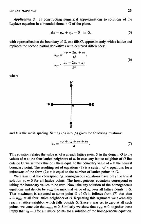
Application 3. In constructing numerical approximations to solutions of theLaplace equation in a bounded domain G of the plane,
Au=u,,+u,.,,=0 in G, (5)
with u prescribed on the boundary of G, one fills G, approximately, with a lattice andreplaces the second partial derivatives with centered differences:
uuw
h'-
uyy -h2
where
W
N
I£
S
and h is the mesh spacing. Setting (6) into (5) gives the following relations:
uW+UN+uE+USun =
4
(6)
(7)
This equation relates the value u of u at each lattice point 0 in the domain G to thevalues of a at the four lattice neighbors of u. In case any lattice neighbor of 0 liesoutside G, we set the value of u there equal to the boundary value of u at the nearestboundary point. The resulting set of equations (7) is a system of n equations for nunknowns of the form (2); n is equal to the number of lattice points in G.
We claim that the corresponding homogeneous equations have only the trivialsolution u = 0 for all lattice points. The homogeneous equations correspond totaking the boundary values to be zero. Now take any solution of the homogeneousequations and denote by umax the maximal value of u over all lattice points in G.That maximum is assumed at some point 0 of G; it follows from (7) that thenu = umax at all four lattice neighbors of 0. Repeating this argument we eventuallyreach a lattice neighbor which falls outside G. Since u was set to zero at all suchpoints, we conclude that u,nax = 0. Similarly we show that um;,, = 0; together theseimply that uO = 0 for all lattice points for a solution of the homogeneous equation.

24 LINEAR ALGEBRA AND ITS APPLICATIONS
By Corollary B', the system of equations (7), with arbitrary boundary data, has aunique solution.
EXERCISE 2. Let
tijxj = Ui, i = 1,...,m
be an overdetermined system of linear equations-that is, the number m of equationsis greater than the number n of unknowns xj, . . . , x,,. Take the case that in spite of theoverdeterminacy, this system of equations has a solution, and assume that thissolution is unique. Show that it is possible to select a subset of n of these equationswhich uniquely determine the solution.
We turn now to the rudiments of the algebra of linear mappings, that is, theiraddition and multiplication. Suppose that T and S are both linear maps of X -> U;then we define their sum T + S by setting for each vector x in X,
(T + S) (x) = Tx + Sx.
Clearly, under this definition T + S is again a linear map of X - U. We define kTsimilarly, and we get another linear map.
It is not hard to show that under the above definition the set of linear mappings ofX -> U themselves forms a linear space. This space is denoted by L(X, U).
Let T, S be maps, not necessarily linear, of X into U, and U into V, respectively, X,U, V arbitrary sets. Then we can define the composition of T with S, a mapping of Xinto Vobtained by letting T act first, followed by S, schematically
V'-U- X.
The composite is denoted by S o T:
S o T(x) = S(T(x)).
Note that composition is associative: if R maps V into Z, then
Ro(SoT)=(RoS)oT.
Theorem 3. (i) The composite of linear mappings is also a linear mapping.(ii) Composition is distributive with respect to the addition of linear maps, that is,
(R+S)oT=RoT+SoT
LINEAR MAPPINGS
and
So(T+P)=SoT+SoP,
25
where R and S map U- V and P and T map X U.
EXERCISE 3. Prove Theorem 3.
On account of this distributive property, coupled with the associative law thatholds generally, composition of linear maps is denoted as multiplication:
SoT ST.
We warn the reader that this kind of multiplication is generally not commutative; forexample, TS may not even be defined when ST is, much less equal to it.
Example 8. X = U = V = polynomials in s, T = d/dc, S = multiplicationby s.
Example 9. X = U = V = R3.
S: rotation around x, axis T: rotation around x2 axisby 90 degrees by 90 degrees
EXERCISE 4. Show that S and T in Examples 8 and 9 are linear and thatST : IS.
Definition. A linear map is called invertible if it is 1-to-1 and onto, that is, if it isan isomorphism. The inverse is denoted as T-I.
EXERCISE 5. Show that if T is invertible, T T- 1 is the identity.
Theorem 4. (i) The inverse of an invertible linear map is linear.(ii) If S and T are both invertible, and if ST is defined, then ST also is invertible,
and
(ST)-' = T-'S-
EXERCISE 6. Prove Theorem 4.
Let T be a linear map X - U, and l a linear function, that is, I is an element of V.Then the product (i.e., composite) IT is a linear mapping of X into K, that is, anelement of X'; denote this element by in:
m(x) = l(Tx). (8)

26 LINEAR ALGEBRA AND ITS APPLICATIONS
This defines an assignment of an element m of X' to every element I of V. It is easyto deduce from (8) that this assignment is a linear mapping U' -+ X'; it is called thetranspose of T and is denoted by V.
Using the notation (6) in Chapter 2 to denote the value of a linear function, we canrewrite (8) as
(m,x) _ (1, Tx). (8')
Using the notation m = T'1, this can be written as
(T'1, x) = (1,Tx). (9)
EXERCISE 7. Show that whenever meaningful,
(ST)'=TS', (T+ R)'=T'+R' and (T-')'=(T')-I.
Example 10. X = I8", U = Rm, T as in Example 7.
U,=Etjxj. (10)
U' is then also 118',X' = 118", with (1, u) = Ei l;u;, (m, x) = E' mixi. Then withu = Tx, using (10) we have
(1, U) _ 1,u; _ litiixlr i
l/t'i/xi=>mixi=(m,x),
where m = T'l, with
nti = l;ty.
EXERCISE 8. Show that if X" is identified with X and U" with U via (5) inChapter 2, then
T" = T.
We shall show in Chapter 4 that if a mapping T is interpreted as a matrix, itstranspose T' is obtained by making the columns of T the rows of T'.
We recall from Chapter 2 the notion of the annihilator of a subspace.

LINEAR MAPPINGS 27
Theorem 5. The annihilator of the range of T is the nullspace of its transpose:
RT = NT,. (12)
Proof. By the definition in Chapter 2 of annihilator, the annihilator of the rangeRT consists of those linear functions I defined on the target space U for which
(!, u) = 0 for all u in RT.
Since u in RT consists of u = Tx, x in X, we can rewrite the above as
(l, Tx) = 0 for all x.
Using (9), we can rewrite this as
(T'!, x) = 0 for all x.
It follows that l is in RT iff T'l = 0; this proves Theorem 5.
Now take the annihilator of both sides of (12). According to Theorem 5 ofChapter 2, the annihilator of Rl is R itself. In this way we obtain the followingtheorem.
Theorem 5'. The range of T is the annihilator of the nullspace of V.
RT = NT,.(12)'
(12)' is a very useful characterization of the range of a mapping. Next we giveanother consequence of Theorem 5.
Theorem 6.
dim RT = dim RT'. (13)
Proof We apply Theorem 4 of Chapter 2 to U and its subspace RT:
dim RT + dim RT = dim U.
Next we use Theorem 2 of this chapter applied to T': U' X':
dim NT, + dim Rr = dim U'.
According to Theorem 2, Chapter 2, dim U = dim U'; according to Theorem 5 ofthis chapter, RT = and so dim RT = dim N. So we deduce (13) from the lasttwo equations.

28 LINEAR ALGEBRA AND ITS APPLICATIONS
The following is an easy consequence of Theorem 6.
Theorem 6'. Let T be a linear mapping of X into U, and assume that X and Uhave the same dimension. Then
dim NT =dimNr. (13)'
Proof. According to Theorem 2, applied to both T and T',
dim NT = dim X - dim RT,
dim Nr = dim U' - dim Rr.
Since dim U = dim U' is assumed to be the same as dim X, (13)' follows from theabove relations and (13). Fl
Theorem 6 is an abstract version of the classical result that the column rank androw rank of a matrix are equal. The usual proofs of this result are abstruse andunclear.
We turn now to linear mappings of a linear space X into itself. The aggregate ofsuch mappings is denoted as 2'(X, X); they are a particularly important andinteresting class of maps. Any two such maps can be added and multiplied, that is,composed, and can be multiplied by a scalar. Thus .f(X, X) is an algebra. Weinvestigate now briefly some of the algebraic aspects of £(X, X).
First we remark that .Y'(X, X) is an associative, but not commutative algebra, witha unit; the role of the unit is played by the identity map I, defined by Ix = x. The zeromap 0 is defined by Ox = 0. £ (X, X) contains divisors of zero, that is, pairs ofmappings S and T whose product ST is 0, but neither of which is 0. To see this,choose T to be any nonzero mapping with a nontrivial nullspace NT, and S to be anynonzero mapping whose range Rs is contained in NT. Clearly, TS = 0.
There are mappings D # 0 whose square D2 is zero. As an example, take X to bethe linear space of polynomials of degree less than 2. Differentiation D maps thisspace into itself. Since the second derivative of every polynomial of degree less than2 is zero, D2 = 0, but clearly D # 0.
EXERCISE 9. Show that if A in ,Y'(X, X) is a left inverse of B in Y(X, X), that isAB = 1, then it is also a right universe: BA = 1.
We have seen in Theorem 4 that the product of invertible elements is invertible.Therefore the set of invertible elements of Y(X,X) forms a group undermultiplication. This group depends only on the dimension of X, and the field K ofscalars. It is denoted as GL(n, K), n = dim X.
Given an invertible element S of 2(X, X), we assign to each M in Y (X, X) theelement Ms constructed as follows:
Ms = SMS-1. (14)

LINEAR MAPPINGS 29
This assignment M -> Ms is called a similarity transformation; M is said to besimilar to Ms.
Theorem 7. (a) Every similarity transformation is an automorphism of L(X,X),maps sums into sums, products into products, scalar multiples into scalarmultiples:
(kM)s = kMs. (15)
(M + K)s = Ms + Ks. (15)'
(MK)s = MSKs. (15)
(b) The similarity transformations form a group.
(MS)T = MTS. (16)
Proof (15) and (15)' are obvious; to verify (15)" we use the definition (14):
MSK5 = SMS-' SKS-' = SMKS-' = (MK)s,
where we made use of the associative law.The verification of (16) is analogous; by (14),
(Ms)T = T(SMS-')T-1 = TSM(TS)-' = MTS;
here we made use of the associative law, and that (TS)-1 = S-'T-1. O
Theorem 8. Similarity is an equivalence relation; that is, it is:
(i) Reflexive. M is similar to itself.(ii) Symmetric. If M is similar to K, then K is similar to M.
(iii) Transitive. If M is similar to K, and K is similar to L, then M is similarto L.
Proof. (i) is true because we can in the definition (14) choose S = I.(ii) M similar to K means that
K = SMS-'. (14)'
Multiply both sides by S on the right and S on the left, and we see that K is similarto M.
(iii) If K is similar to L, then
L=TKT-', (14)"
30 LINEAR ALGEBRA AND ITS APPLICATIONS
where T is some invertible mapping. Multiply both sides of (14)' by T-1 on the rightand by on the left; we get
TKT-' = TSMS-T-'.
According to (14)", the left-hand side is L. The right-hand side can be written as
(TS) M(TS)_',
which is similar to M.
EXERCISE 10. Show that if M is invertible, and similar to K, then K also isinvertible, and K-I is similar to M.
Multiplication in £(X, X) is not commutative, that is, AB is in general not equalto BA. Yet they are not totally unrelated.
Theorem 9. If either A or B in .'(X, X) is invertible, then AB and BA aresimilar.
EXERCISE 11. Prove Theorem 9.
Given any element A of .2'(X, X) we can, by addition and multiplication, form allpolynomials in A:
aNAN +av_1 AN-i +... +aol;
we can write (17) as p(A), where
Vp(s) = aNS + ... + ao.
(17)
(17)'
The set of all polynomials in A forms a subalgebra of 2'(X, X); this subalgebra iscommutative. Such commutative subalgebras play a big role in spectral theory,discussed in Chapters 6 and 8.
An important class of mappings of a linear space X into itself are projections.
Definition. A linear mapping P: X -> X is called a projection if it satisfies
PZ = P.
Example 11. X is the space of vectors x = (a1, aZ, ... , a"), P defined as
Px = (0, 0,
That is, the action of P is to set the first two components of x equal to zero.
LINEAR MAPPINGS 31
EXERCISE 12. Show that P defined above is a linear map, and that it is aprojection.
Example 12. Let X be the space of continuous functions f in the interval [-1, 1];define Pf to be the even part off, that is,
(Pf)(x)=.f(x) +f(-x)
2
EXERCISE 13. Prove that P defined above is linear, and that it is a projection.
Definition. The commutator of two mappings A and B of X into X is AB-BA.Two mappings of X into X commute if their commutator is zero.
Remark. We can prove Corollary A' directly by induction on the number ofequations in, using one of the equations to express one of the unknowns xj in terms ofthe others. By substituting this expression for xx into the remaining equations, wehave reduced the number of equations and the number of unknowns by one.
The practical execution of such a scheme has pitfalls when the number ofequations and unknowns is large. One has to pick intelligently the unknown to beeliminated and the equation that is used to eliminate it. We shall take up thesematters in the next chapter.
Definition. The rank of a linear mapping is the dimension of its range.
EXERCISE 14. Suppose T is a linear map of rank I of a finite dimensional vectorspace into itself.
(a) Show there exists a unique number c such that T2 = cT.(b) Show that if c # 1 then I-T has an inverse. (As usual I denotes the identity
map Ix = x.)
EXERCISE 15. Suppose T and S are linear maps of a finite dimensional vectorspace into itself. Show that the rank of ST is less than or equal the rank of S. Showthat the dimension of the nullspace of ST is less than or equal the sum of thedimensions of the nullspaces of S and of T.
CHAPTER 4
Matrices
In Example 7 of Chapter 3 we defined a class of mappings T: R" -> U8m where theith component of u = Tx is expressed in terms of the components xl of x by theformula
u( tjlxl, t = l , ... , to (1)
and the tjl are arbitrary scalars. These mappings are linear; conversely, we have thefollowing theorem.
Theorem 1. Every linear map Tx = u from R" to R' can be written in form (1).
Proof. The vector x can be expressed as a linear combination of the unit vectorse1, ... , e where ej has jth component 1, all others 0:
x = E xlel. (2)
Since T is linear
u=Tx=>xjTel. (3)
Denote the ith component of Tel by tjl:
tij = (Tel);. (4)
Linear Algebra and Its Applications, Second Edition, by Peter D. LaxCopyright R) 2007 John Wiley & Sons, Inc.
32

MATRICES
It follows from (3) and (4) that the ith component u, of It is
Ui = xjtij,
exactly as in formula (1).
33
It is convenient and traditional to arrange the coefficients tij appearing in (1) in arectangular array,
t1I t12 ... tin
121
t,n! ... taw
(5)
Such an array is called an m by n (m x n) matrix, m being the number of rows,n the number of columns. A matrix that has the same number of rows andcolumns is called a square matrix. The numbers tij are called the entries of thematrix T.
According to Theorem 1, there is a 1-to-I correspondence between m x nmatrices and linear mappings T: Ifs" -> R"'. We shall denote the (ij)th entry tij of thematrix identified with T by
Tij = (T)ij. (5)'
A matrix T can be thought of as a row of column vectors, or a column of rowvectors:
ri
T = (ci,...,cn) _r,,,
cj = ri = (tii,...,tin) (6)
According to (4), the ith component of Tej is tij; according to (6), the ith componentof cj is tij. Thus
Tej = cj. (7)
This formula shows that, as consequence of the decision to put tij in the ith row andjth column, the image of ej under T appears as a column vector. To be consistent, weshall write all vectors in U = 68as column vectors:
ui
um

34 LINEAR ALGEBRA AND ITS APPLICATIONS
We shall also write elements of X = I8" as column vectors:
x=
The matrix representation (6) of a linear map l from 118" to I is a single row vectorof n components:
(8)
We define by (8) the product of a row vector r with a column vector x, in this order. Itcan be used to give a compact description of formula (1) giving the action of a matrixon a column vector:
rixTx=
r,,,X
(9)
where r 1 , . . . , r,,, are the rows of the matrix T.In Chapter 3 we have described the algebra of linear mappings. Since matrices
represent linear mappings of 118"` into I8", there is a corresponding algebra of matrices.Let S and T be m x n matrices, representing mappings of 118"' to I8'. Their sum
T + S represents the sum of these mappings. It follows from formula (4) that theentries of T + S are the sums of the corresponding entries of T and S:
(T + S)ij = Tij + Sij.
Next we show how to use (8) and (9) to calculate the elements of the product oftwo matrices. Let T, S be matrices
T: I8" -> 118', S: I8m -> Ri.
Since the target space of T is the domain space of S, the product ST is well-defined.According to formula (7) applied to ST, the jth column of ST is
STej.
According to (7), Tej = cj; applying (9) to x = Tej, and S in place of T gives
sIcj
STej = Scj =
sjcj
where sk denotes the kth row of S. Thus we deduce this rule:

MATRICES 35
Rule of matrix multiplication. Let T be an m x n matrix and S an 1 x in matrix.Then the product of ST is an 1 x n matrix whose (kj)th entry is the product of the kthrow of S and the jth column of T:
(ST)kj = SkCj,
where sk is the kth row of S and cj is the jth column of T.In terms of entries,
Example 1.
Example 2.
Example 3.
Example 4.
Example 5.
Example 6.
Example 7.
(ST ),j = SkiTij.
2 5 6 19 22(3
1
4) (7 8) - (43 50)
()(3 4) = (6 8).
(3
(I
5(3
4)(2)=(11).
2)(5 6)=(13 16).
6)(2) _
(1 (1 2)
(1 2) (56)(21)
= (13 16) (2) = (45);
5C77 6
8) (3 4) -(23
46)
(10)
(10)'
Examples 1 and 7 show that matrix multiplication of square matrices need not becommutative. Example 6 is an illustration of the associative property of matrixmultiplication.
EXERCISE I. Let A be an arbitrary m x n matrix, and let D be an m x ndiagonal matrix,
_ d, ifi=j,D' 0 if i#j.

36 LINEAR ALGEBRA AND ITS APPLICATIONS
Show that the ith row of DA equals d, times the ith row of A, and show that the jthcolumn of AD equals dj times the jth column of A.
An n x n matrix A represents a mapping of [l8" into R". If this mapping isinvertible, the matrix A is called invertible.
Remark. Since the composition of linear mappings is associative, matrixmultiplication, which is the composition of mappings from 68" to liwith mappingsfrom 1 m to R', also is associative.
We shall identify the dual of the space R' of all column vectors with ncomponents as the space (R")' of all row vectors with n components.
The action of a vector I in the dual space (R")' on a vector x of fl8", denotedby brackets in formula (6) of Chapter 2, shall be taken to be the matrixproduct (8):
(11)
Let x, T and I be linear mappings as follows:
1: R' -+ 1, T: 08" -, R', x: R->R".
According to the associative law,
(lT)x = I(Tx). (12)
We identify I with an element of (Rand IT with an element of (11")'. Using thenotation (11) we can rewrite (12) as
(IT,x) = (1,Tx). (13)
We recall now the definition of the transpose T' of T, defined by formula (9) ofChapter 3,
(T'l,x) = (1,Tx). (13)'
Comparing (13) and (13)' we see that the matrix T acting from the right on rowvectors is the transpose of the matrix T acting from the left on column vectors.
To represent the transpose Vas a matrix acting on column vectors, we change itsrows into columns, its columns into rows, and denote the resulting matrix as TT:
(TT)ij = Tj;. (13)"
Given a row vector r = (rj, . . . , we denote by rT the column vector with thesame components. Similarly, given a column vector c, cT denotes the row vector withthe same components.
MATRICES 37
Next we turn to expressing the range of T in matrix language. Setting (7),cj = Ti, finto (3), Tx = E xjTel, gives
u=Tx=x1ci+
This gives the following theorem.
Theorem 2. The range of T consists of all linear combinations of the columnsof the matrix T.
The dimension of this space is called in old-fashioned texts the column rank of T.The row rank is defined similarly; (13)" shows that the row rank of T is thedimension of the range of TT. Since according to Theorem 6 of Chapter 3.
dim RT = dim RTT,
we conclude that the column rank and row rank of a matrix are equal.
EXERCISE 2. Look up in any text the proof that the row rank of a matrix equalsits column rank, and compare it to the proof given in the present text.
We show now how to represent a linear mapping T: X -> U by a matrix. We haveseen in Chapter 1 that X is isomorphic to li", n = dim X, and U isomorphic to t',m = dim U. The isomorphisms are accomplished by choosing a basis in X,y, , ... , y,,, and then mapping yf f-, ej, j = l .... , n:
B: X-+R"; (14)
similarly,
C: U R"'. (14)'
Clearly, there are as many isomorphisms as there are bases. We can use any of theseisomorphisms to represent T as ifs" -> aB, obtaining a matrix representation M:
CTB-' = M. (15)
When T is a mapping of a space X into itself, we use the same isomorphism in(14) and (14)', that is, we take B = C. So in this case the matrix representing T hasthe form
BTB-' = M. (15)'

38 LINEAR ALGEBRA AND ITS APPLICATIONS
Suppose we change the isomorphism B. How does the matrix representing Tchange? If C is another isomorphism X H", the new matrix N representing T isN = CTC-1. We can write, using the associative rule and (15)',
N = CTC-1 = CB-'BTB-IBC-1 = SMS-1, (16)
where S = CB-1. Since B and C both map X into H", CB-' = S maps H" onto H",that is, S is an invertible n x it matrix.
Two square matrices N and M related to each other as in (16) are calledsimilar. Our analysis shows that similar matrices describe the same mapping of aspace into itself, in different bases. Therefore we expect similar matrices to havethe same intrinsic properties; we shall make the meaning of this more precise inChapter 6.
We can write any n x n matrix A in 2 x 2 block form:
A = All A12\'A21 A22
where A11 is the submatrix of A contained in the first k rows and columns, A12 thesubmatrix contained in the first k rows and the last n - k columns, and so on.
EXERCISE 3. Show that the product of two matrices in 2 x 2 block form can beevaluated as
All A12 B11 B12 _ AIIBII+A12B21 A11B12+A12B22A21 A22 B21 B22) AN B 11 + A22B21 AN B 12 + A22B22 )
The inversion of matrices will be discussed from a theoretical point of view inChapter 5, and from a numerical point of view in Chapter 17.
A matrix that is not invertible is called singular.
Definition. The square matrix 1 whose elements are lij = 0 when i islu = I is called the unit matrix.
54 j,
Definition. A square matrix (t,,) for which tip = 0 for i > j is called uppertriangular. Lower triangular is defined similarly.
Definition. A square matrix (tip) for which tq = 0 when I i - ji > I is calledtridiagonal.
EXERCISE 4. Construct two 2 x 2 matrices A and B such that AB = 0 butBA#0.

MATRICES 39
We turn now to the most important, certainly the oldest, way to solve sets of linearequations, Gaussian elimination. We illustrate it on a simple example of four linearequations for four unknowns x1, x2, x3, and x4:
xj + 2x2 + 3x3 - x4 = -2,2xi + 5x2 + 4X3 - 3x4 = 1,
2x, + 3x2 + 4x3 + x4 = 1,
x1 +4x2+2x3-2x4 =3.
(17)
We solve this system of equations by eliminating the unknowns one by one; here ishow it is done. We use the first equation in (17) to eliminate xi from the rest of theequations. To accomplish this, subtract two times the first equation from the secondand the third equations, obtaining
x2-2x3-x4=5, (18),
and
-x2-2x3+3x4=5. (18)2
Subtract the first equation from the fourth one, obtaining
2x2 - X3 - x4 = 5. (18)3
We use the same technique to eliminate x2 from the set of three equations (18).We obtain
-4x3 + 2x4 = 10,
3X3 + X4 = -5.
(19),
(19)2
Finally we eliminate x3 from equations (19) by adding 3/4 times (19), to (19),; weget
2x4 = 5/2,
which yields
x4 = 1. (20)4
We proceed in the reverse order, by backward substitution, to determine the otherunknowns. Setting the value of x4 from (20)4 into equation (19), gives
-4x3+2= 10..

40 LINEAR ALGEBRA AND ITS APPLICATIONS
which yields
X3=-2. (20)3
We could have used equation (19)2 and would have gotten the same answer.We determine x2 from any of the equations (18), say (l8) i, by using (20)3 and
(20)4 for X3 and x4. We get
x2+4- 1 =5,
so
x2 = 2. (20)2
Finally we determine xi from, say, the first equation (17), using the previouslydetermined values of X4, X3, and x2:
xi+4-6-1=-2,xi = 1. (20),
EXERCISE 5. Show that xi, X2, X3, and x4 given by (20), satisfy all four equations(20).
Notice that the order in which we eliminate the unknowns, along with theequations which we use to eliminate them, is arbitrary. We shall return to thesepoints.
A system of n equations
n (21)
for n unknowns xi , .... x,, may have a unique solution, may have no solution, or mayhave many solutions. We show now how to use Gaussian elimination to determine allsolutions, or conclude that no solution exists. Here is an example that illustrates thelast two possibilities.
xI + X2 + 2x3 + 3x4 = ui,
xj + 2x2 + 3x3 + X4 = U2,
2xi + X2 + 2X3 + 3x4 = u3i
3xi + 4x2 + 6X3 + 2x4 = u4.
(22)

MATRICES 41
We eliminate x, from the last three equations by subtracting from them anappropriate multiple of the first equation:
X2 +X3-2X4=U2-U,-X2 - 2X3 - 3X4 = U3 - 2u,
X2-7x4=U4- 3u,
We use the first equation above to eliminate x2 from the last two:
-X3 - 5x4 = U3 + U2 - 3u,
-X3 - 5X4 = U4 - U2 - 2u,
We eliminate x3 by subtracting the last two equations from each other. We find thatthereby we have eliminated x4 as well, and we get
0 = U4 - U3 - 2U2 + U,. (23)
This is the necessary and sufficient condition for the system of equations (22) to havea solution.
EXERCISE 6. Choose values of u,, u2, U3, u4 so that condition (23) is satisfied,and determine all solutions of equations (22).
Equation (22) can be written in matrix notation as
Mx = U, (22)'
where x and u are column vectors with components x,, x2, X3, x4 and u,, u2, u3, U4,and
1 2 3 1
2 1 2 3
3 4 6 2
EXERCISE 7. Verify that l = (1, -2, -1, 1) is a left nullvector of M:
/M=0.
Multiply equation (22)' on the left by l; using the result of Exercise 7, we get that
IMx=1u=0,
a rederivation of (23) as a necessary condition for (22)' to have a solution.
42 LINEAR ALGEBRA AND ITS APPLICATIONS
EXERCISE 8. Show by Gaussian elimination that the only left nuilvectors of Mare multiples of I in Exercise 7, and then use Theorem 5 of Chapter 3 to show thatcondition (23) is sufficient for the solvability of the system (22).
Next we show how to use Gaussian elimination to prove Corollary A' inChapter 3:
A system of homogeneous linear equations
tjxj=0, i= 1...... m,j=1
(24)
with fewer equations than unknowns, in < n, has a nontrivial solution-that is, onewhere at least one of the xj is nonzero.
Proof. We use one of the equations (24) to express x, as a linear function of therest of the x's:
XI = 11(x2,...,X.). (25),
We replace x, by 11 in the remaining equations, and we use one of them to express x2as a linear function of the remaining x's:
X2 = !2(X3,...xn).
We proceed in this fashion until we reach x:
xu, = lm(Xm+1 . . . . . x ) .
(25)2
(25)m
Since there were only in equations and in < n, there are no more equations left to besatisfied. So we choose the values of x,,,+1 , . . . , x, arbitrarily, and we use equations(25),,,, (25).-1.... , (25)1, in this order, to determine the values of x,,,, xm_,, ... ,X1.
This procedure may break down at the ith step if none of the remaining equationscontain xi. In this case we set x;.,1, ... ,x equal to zero, assign an arbitrary value toxi, and determine x;_1,.... x, from equations (25)i_1,...,(25)1, in thisorder. M
We conclude this chapter with some observations on how Gaussian eliminationworks for determined systems of n inhomogeneous equations
tijxj = u;, i = 1,...,nj=1
(26)
for n unknowns . . . . . x .,. In its basic form the first equation is used to eliminate x, ,that is, express it as
x, = (27)1

MATRICES 43
Then x, is replaced in the remaining equations by v, + 11. The first of these equationsis used to express x2 as
X2 = V2 + 12(X3,...,x,)- (27),
We proceed in this fashion until after (n - 1) steps we find the value of x,,. Then wedetermine the values of 1 i ... , xl , in this order, from the relations
This procedure may break down right at the start if the coefficient t11 of x, in thefirst equation is zero. Even if t,1 is not zero but very small, using the first equation toexpress x, in terms of the rest of the x's involves division by t,1 and produces verylarge coefficients in formula (27). This wouldn't matter if all arithmetic operationswere carried out exactly, but they never are; they are carried out in finite digitfloating point arithmetic, and when (27)1 is substituted in the remaining equations,the coefficients ty, i > 1, are swamped.
A natural remedy is to choose another unknown, x1, for elimination and anotherequation to accomplish it, so chosen that t;j is not small compared with the othercoefficients. This strategy is called complete pivoting and is computationallyexpensive. A compromise is to keep the original order of the unknowns forelimination, but use another equation for elimination, for which t;, is not smallcompared to the other coefficients. This strategy, called partial pivoting, works verywell in practice (see, e.g., the text entitled Numerical Linear Algebra, by Trefethenand Bau.)

CHAPTER 5
Determinant and Trace
In this chapter we shall use the intuitive properties of volume to define thedeterminant of a square matrix. According to the precepts of elementary geometry,the concept of volume depends on the notions of length and angle and, in particular,perpendicularity, concepts that will be defined only in Chapter 8. Nevertheless, itturns out that volume is independent of all these things, except for an arbitrarymultiplicative constant that can be fixed by specifying that the unit cube havevolume one.
We start with the geometric motivation and meaning of determinants. A simplexin ll8" is a polyhedron with n + 1 vertices. We shall take one of the vertices to be theorigin and denote the rest as a 1 , . . . , a,,. The order in which the vertices are takenmatters, so we call 0, a i , .... a,, the vertices of an ordered simplex.
We shall be dealing with two geometrical attributes of ordered simplices, theirorientation and volume. An ordered simplex S is called degenerate if it lies on an(n - 1)-dimensional subspace.
An ordered simplex (0, at, ... , S that is nondegenerate can have one of twoorientations: positive or negative. We call S positively oriented if it can be deformedcontinuously and nondegenerately into the standard ordered simplex (0, et,... , en),where ej is the jth unit vector in the standard basis of R". By such deformation wemean n vector-valued continuous functions al(t) of t,0 < t < 1, such that (i)S(t) = (0, at (t), ... , an(t)) is nondegenerate for all t and (ii) aa(0) = aa, aj(1) = ej.Otherwise S is called negatively oriented.
For a nondegenerate oriented simplex S we define O(S) as + 1 or -1, dependingon the orientation of S, and zero when S is degenerate.
The volume of a simplex is given by the elementary formula
Vo1(S) =1
Vol,,_ 1(Base)Altitude.n
Linear Algebra and Its Applications, Second Edition, by Peter D. LaxCopyright ((; 2007 John Wiley & Sons, Inc.
(1)
44
DETERMINANT AND TRACE 45
By base we mean any of the (n - 1)-dimensional faces of S, and by altitude we meanthe distance of the opposite vertex from the hyperplane that contains the base.
A more useful concept is signed volume, denoted as E(S), and defined by
E(S) = O(S)Vol(S). (2)
Since S is described by its vertices, 2(S) is a function of a1,. .. , a,,. Clearly, whentwo vertices are equal, S is degenerate, and therefore we have the following:
(i) E(S) = 0 if aj =ak, j¢k.A second property of E(S) is its dependence on aj when the other vertices are
kept fixed:(ii) E(S) is a linear function of ai when the other ak, k # j , are kept fixed.
Let us see why we combine formulas (1) and (2) as
>(S) = 1n
where
k = O(S)Altitude.
The altitude is the distance of the vertex a1; we call k the signed distance of thevertex from the hyperplane containing the base, because O(S) has one sign when ajlies on one side of the base and the opposite sign when aj lies on the opposite side.
We claim that when the base is fixed, k is a linear function of aa. To see why this isso we introduce Cartesian coordinate axes so that first axis is perpendicular to thebase and the rest lie in the base plane. By definition of Cartesian coordinates, the firstcoordinate k, (a) of a vector a is its signed distance from the hyperplane spanned bythe other axes. According to Theorem I (i) in Chapter 2, k, (a) is a linear function ofa. Assertion (ii) now follows from formula (1)'.
Determinants are related to the signed volume of ordered simplices by theclassical formula,
E (S) = I D(a,, ... , a ), (3)
where D is the abbreviation of the determinant whose columns are a, , . . . , a,,. Ratherthan start with a formula for the determinant, we shall deduce it from the propertiesforced on it by the geometric properties of signed volume. This approach todeterminants is due to E. Artin.
Property(i). D(a, , ... , 0 if a; = aj, i 0 j.

46 LINEAR ALGEBRA AND ITS APPLICATIONS
Property (ii). D(a1, ... , a multilinear function of its arguments, in thesense that if all a;, i # j are fixed, D is a linear function of the remainingargument al.
Property (iii). Normalization:
D(e, , ... , en) = 1. (4)
We show now that all remaining properties of D can be deduced from those so farpostulated.
Property (iv). D is an alternating function of its arguments, in the sense that ifai and aj are interchanged, i # j, the value of D changes by the factor (- 1).
Proof. Since only the ith andjth argument change, we shall indicate only these.Setting a; = a, aj = h we can write, using Properties (i) and (ii):
D(a, b) = D(a, b) + D(a, a) = D(a, a + b)
= D(a,a+b) - D(a+b, a+b)= -D(b, a + b) = -D(b, a) - D(b, b) = -D(b, a).
Property (v). If a, , ... , an are linearly dependent, then D(a,.... , 0.
Proof. If as,. .. , a are linearly dependent, then one of them, say a,, can beexpressed as a linear combination of the others:
a, = k2a2 + .. +
Then, using Property (ii),
D(a,.... ,an) = D(k2a2+... +knana a2,....k2D(a2, a2, -,an) + ... + knD(an, a2, .... an).
By property (i), all terms in the last line are zero.
Next we introduce the concept of permutation. A permutation is a mapping p of nobjects, say the numbers 1, 2. ... , n, onto themselves. Like all functions,permutations can be composed. Being onto, they are one-to-one and so can beinverted. Thus they form a group; these groups, except for n = 2, arenoncommutative.
We denote p(k) as pk; it is convenient to display the action of p by a table:
1 2 n

DETERMINANT AND TRACE 47
Example 1. p = 2433. Then
2 _ 1234 i = 1234P
4321'P
3142'
3 _ 1234 a _ 1234
p 3142p
1234.
Next we introduce the concept of signature of a permutation, denoted as a(p). Letxi, ... , x,, be n variables; their discriminant is defined to be
P(xi,...,x,) = fJ(xi - xj).
i<j
Let p be any permutation. Clearly,
rl(xpi - xnj)1<j
is either P(xi,...x,,) or
Definition. The signature 6(p) of a permutation p is defined by
P(p(xi,...,xn)) = Or(p)P(xi,...,xn).
Properties of signature:
(a) a(p) = +I or - 1.(b) o'(Pi oP2) = a(p1)o'(p2)
EXERCISE I. Prove properties (7).
(5)
(6)
(7)
We look now at a special kind of permutation, an interchange. These are definedfor any pair of indices, j, k, j # k as follows:
p(i) = i fori # fork,
p(j) = k, p(k) =j.
Such a permutation is called a transposition. We claim that transposition has thefollowing properties:
(c) The signature of a transposition t is minus one:
a(t) = -1. (8)
(d) Every permutation p can be written as a composition of transpositions:
,) = tk 0 ... 0 ti. (9)

48 LINEAR ALGEBRA AND ITS APPLICATIONS
EXERCISE 2. Prove (c) and (d) above.
Combining (7) with (8) and (9) we get that
a(P) = (-1)k, (10)
where k is the number of factors in the decomposition (9) of p.
EXERCISE 3. Show that the decomposition (9) is not unique, but that the parityof the member k of factors is unique.
Example 2. The permutation p = ?4545 is the product of three transpositions11 = 12345 t2 = 12345 t3 = 12345:
12543 21345 42315
p=t3012 0 I
We return now to the function D. Its arguments aj are column vectors
a IJ
aJ= 1,...,n.
This is the same as
aj = aljel + ... +
Using Property (ii), multilinearity, we can write
D(al,...,an) = D(allel + ... + anIe,,,a2,...,an)
= all D(e1, a2, ... , an) + ... + a,I D(en, a2, ... , an). (12)
Next we express a2 as a linear combination of el.... , e and obtain a formula like(12) but containing n22 terms. Repeating this process n times we get
D(al.... ,an) _ at,l aj2...afn D(ef..... ef), (13)f
where the summation is over all functions f mapping 11, . . . , n} into { I.... , n}.If the mapping f is not a permutation, then f; = f for some pair i # j and byProperty (i).
D(ef,..... ef) = 0. (14)
This shows that in (13) we need sum only over those f that are permutations.We saw earlier that each permutation can be decomposed into k transpositions
(9). According to Property (iv), a single transposition of its arguments changes the

DETERMINANT AND TRACE 49
value of D by a factor of (-1). Therefore k transpositions change it by the factor(-1)k. Thus, using (10),
D(ee,,...,en,)=a(P)D(e,,...,e,,) (15)
for any permutation. Setting (14) and (15) into (13) we get, after using thenormalization (4), that
D(ai,...,a,.) = Ea(P)an i ...ap.,,. (16)
This is the formula for D in terms of the components of its arguments.Formula (16) was derived using solely properties (i), (ii), and (iii) of
determinants. Therefore we conclude with the following theorem.
Theorem 1. Properties (i), (ii), and (iii) uniquely determine the determinant asa function of a, , . . . ,
EXERCISE 4. Show that D defined by (16) has Properties (ii), (iii) and (iv).
EXERCISE 5. Show that Property (iv) implies Property (i), unless the field K hascharacteristic two, that is, 1 + I = 0.
Definition. Let A be an n x n matrix; denote its column vectors bya,,. -., a,,: A = (at,... , a,,). Its determinant, denoted as det A, is
det A = D(a,,...,a,,), (17)
where D is defined by formula (16).
The determinant has properties (i)-(v) that have been derived and verified for thefunction D. We state now an additional important property.
Theorem 2. For all pairs of n x n matrices A and B,
det(BA) = det A det B. (18)
Proof. According to equation (7) of Chapter 4, the jth column of BA is (BA)ee.The jth column aj of A is Aej; therefore the jth column of BA is
(BA)ej = BAe1 = Bad.
By definition (17),
det(BA) = D(Ba,,... , (19)
50 LINEAR ALGEBRA AND ITS APPLICATIONS
We assume now that det B # 0 and define the function C as follows:
det(BA)
Using (19) we can express C as follows:
detB
(20)
(20)'
We claim that the function C has Properties (i)-(iii) postulated for D.(i) If a; = aj, i # j, then Ba; = Baj; since D has Property (i), it follows that the
right-hand side of (20)' is zero. This shows that C also has Property (i).(ii) Since Ba; is a linear function of a;, and since D is a multilinear function,
it follows that the right-hand side of (20)' is also a multilinear function. This showsthat C is a multilinear function of a I, . . . , a,,, that is, has Property (ii).
(iii) Setting a; = e;, i = 1, 2 , ... , n into formula (20)', we get
D(Be1..... Be,,)detB
Now Be; is the ith column b, of B, so that the right-hand side of (21) is
D(bi,...,b")
det B
(21)
(22)
By definition (17) applied to B, (22) equals I; setting this into (21) we see thatC(ei .... , e") = 1. This proves that C satisfies Property (iii).
We have shown in Theorem I that a function C that satisfies Properties (i)-(iii) isequal to the function D. So
D(ai,....a,,) = detA.
Setting this into (20) proves (18), when det B 54 0.When det B = 0 we argue as follows: define the matrix B(t) as
B(t)=B+tI.
Clearly, B(0) = B. Formula (16) shows that D(B(t)) is a polynomial of degree n, andthat the coefficient of t" equals one. Therefore, D(B(t)) is zero for no more than nvalues of t; in particular D(B(t)) 0 for all t near zero but not equal to zero.According to what we have already shown, det(B(t)A) = det A det B(t) for all suchvalues of t; letting i tend to zero yields (18). El
DETERMINANT AND TRACE
Corollary 3. Ann x n matrix A is invertible if det A # 0.
51
Proof. Suppose A is not invertible; then its range is a proper subspace of R". Therange of A consists of all linear combinations of the columns of A; therefore thecolumns are linearly dependent. According to property (v), this implies thatdet A = 0.
Suppose, on the other hand, that A is invertible; denote its inverse by B:
BA=1.
According to Theorem 2
det B det A = det 1.
By property (iii), det I = 1; so, since D(1) = 1,
det B det A= 1,
which shows that det A # 0.
The geometric meaning of the multiplicative property of determinants is this: thelinear mapping B maps every simplex onto another simplex whose volume is Idet BItimes the volume of the original simplex. Since every open set is the union ofsimplices, it follows that the volume of the image under B of any open set is Idet BItimes the original volume.
We turn now to yet another property of determinants. We need the followinglemma.
Lemma 4. Let A be an n x n matrix whose first column is el:
I X X X0
A= A0
(23)
here All denotes the (n - 1) x (n - 1) submatrix formed by entries ay, i > I, j > 1.We claim that
det A = det A,,. (24)
Proof As first step we show that
1 0...0det A = det 0 All (25)
0

52 LINEAR ALGEBRA AND ITS APPLICATIONS
For it follows from Properties (i) and (ii) that if we alter a matrix by adding amultiple of one of its columns to another, the altered matrix has the samedeterminant as the original. Clearly, by adding suitable multiplies of the first columnof A to the others we can turn it into the matrix on the right in (25).
We regard now
C(AII) = detC1 0 1
0 All
as a function of the matrix All. Clearly it has Properties (i)-(iii). Therefore it mustbe equal to det A,,. Combining this with (25) gives (24).
EXERCISE 6. Verify that C(AII) has properties (i)-(iii).
Corollary 5. Let A be a matrix whose jth column is e;. Then
detA = (25)'
where A,, is the (n - 1) x (n - 1) matrix obtained by striking out the ith row and jthcolumn of A; A; is called the (ij)th minor of A.
EXERCISE 7. Deduce Corollary 5 from Lemma 4.
We deduce now the so-called Laplace expansion of a determinant according to itscolumns.
Theorem 6. Let A be any n x n matrix and j any index between I and n.Then
det A = (-1)'+'a1 det (26)
Proof. To simplify notation, we take j = I. We write aI as a linear combinationof standard unit vectors:
al =allel
Using multilinearity, we get
detA = D(al,...,an) =D(allelalID(el,a2,...,an) + ..
Using Corollary 5, we obtain (26).

DETERMINANT AND TRACE 53
We show now how determinants can be used to express solutions of systems ofequations of the form
Ax = u, (27)
A an invertible n x n matrix. Write
x=Exjej;
according to (7) of Chapter 4, Ae; = aj, the jth column of A. So (27) is equivalent to
E xjaj = u. (27)'j
We consider now the matrix Ak obtained by replacing the kth column of A by u:
Ak = (al.... ,ak-I, u,ak+I,...,a,,)
= (a1,...,ak-I, Exjaj,ak+I,.... a,).
We form the determinant and use its multilinearity,
detAk = xjdet(al,...,ak-I, aj, ak+I.... ,an).
Because of Property (i) of determinants, the only nonzero term on the right is the kth,so we get
det Ak = xk det A.
Since A is invertible, det A 0; so
det AkXk =
det A(28)
We use now the Laplace expansion of det Ak according to its kth column; we get
det Ak = (-1),+k det A;ku;
and so, using (28),
Xk = 1)i+kdetA,ku, (29)det A
54 LINEAR ALGEBRA AND ITS APPLICATIONS
This is called Cramer's rule for finding the solution of the system of equations (27).We now translate (29) into matrix language.
Theorem 7. The inverse matrix A-' of an invertible matrix A has the form
+,F det A;k('4 )k; _ (-1) det A
(30)
Proof. Since A is invertible, det A 0. A-1 acts on the vector u; see formula (1)of Chapter 4,
(A-'u)k = (A-')k;u, (31)
Using (30) in (31) and comparing it to (29) we get that
that is,
(A- Iu)k = Xk, k = 1,...,n, (32)
A-lu = x.
This shows that A-' as defined by (30) is indeed the inverse of A whose action isgiven in (27). p
We caution that reader that for n > 3, formula (30) is not a practical numericalmethod for inverting matrices.
EXERCISE 8. Show that for any square matrix
det AT = det A, AT = transpose of A. (33)
[Hint: Use formula (16) and show that for any permutation Q(p) = v(p-I ).]
EXERCISE 9. Given a permutation p of n objects, we define an associated so-called permutation matrix P as follows:
1, if j = p(i),P; _0, otherwise.
(34)
Show that the action of P on any vector x performs the permutation p on thecomponents of x. Show that if p, q are two permutations and P, Q are the associatedpermutation matrices, then the permutation matrix associated with poq is the productPQ.
DETERMINANT AND TRACE 55
The determinant is an important scalar-valued function of n x n matrices.Another equally important scalar-valued function is the trace.
Definition. The trace of a square matrix A, denoted as tr A, is the sum of theentries on its diagonal:
tr A = aii. (35)
Theorem 8. (a) Trace is a linear function:
trkA =ktrA, tr(A+B) =trA+trB.
(b) Trace is "commutative"; that is,
tr(AB) = tr(BA) (36)
for any pair of matrices.
Proof Linearity is obvious from definition (35). To prove part (b), we use therule, [see (10)' of Chapter 4] for matrix multiplication:
(AB)ii = aikbkik
and
(BA)ii = E bikakik
So
tr(AB) = > aikbki = E bikaki = tr(BA)it i,k
follows if one interchanges the names of the indices i, k.
We recall from the end of Chapter 3 the notion of similarity. The matrix A iscalled similar to the matrix B if there is an invertible matrix S such that
A = SBS-'. (37)
We recall from Theorem 8 of Chapter 3 that similarity is an equivalence relation;that is, it is the following:
(i) Reflexive: A is similar to itself.(ii) Symmetric: if A is similar to B, B is similar to A,
(iii) Transitive: if A is similar to B, and B is similar to C, then A is similar to C.

56 LINEAR ALGEBRA AND ITS APPLICATIONS
Theorem 9. Similar matrices have the same determinat and the same trace.
Proof. Using Theorem 2, we get from (37)
detA = (det S)(det B)(det S-1) = (det B)(det S) det(S-1)
= detB det(SS-1) = (detB)(detI) = detB.
To show the second part we use Theorem 7(b):
trA = tr(SBS-) = tr((SB)S-') = tr(S-'(SB)) = trB. O
At the end of Chapter 4 we remarked that any linear map T of an n-dimensionallinear space X into itself can, by choosing a basis in X, be represented as an n x nmatrix. Two different representations, coming from two different choicesof bases, are similar. In view of Theorem 9, we can define the determinantand trace of such a linear map T as the determinant and trace of a matrixrepresenting T.
EXERCISE to. Let A be an m x n matrix, B an n x m matrix. Show that
trAB = trBA.
EXERCISE I I. Let A be an n x n matrix, AT its transpose. Show that
trAAT = E a .
The square root of the double sum on the right is called the Euclidean, or Hilbert-Schmidt, norm of the matrix A.
In Chapter 9, Theorem 4, we shall derive an interesting connection betweendeterminant and trace.
EXERCISE 12. Show that the determinant of the 2 x 2 matrix
is D = ad - bc.
EXERCISE 13. Show that the determinant of an upper triangular matrix, onewhose elements are zero below the main diagonal, equals the product of its elementsalong the diagonal.
DETERMINANT AND TRACE 57
EXERCISE 14. How many multiplications does it take to evaluate det A by usingGaussian elimination to bring it into upper triangular from?
EXERCISE 15. How many multiplications does it take to evaluate det A byformula (16)?
EXERCISE 16. Show that the determinant of a (3 x 3) matrix
fa b cA= d e f
g h i
can be calculated as follows. Copy the first two columns of A as a fourth and fifthcolumn:
a b c a b
d e f d eg h i g h
det A=aei+bfg+cdh-gec-hfa-idb.
Show that the sum of the products of the three entries along the dexter diagonals,minus the sum of the products of the three entries along the sinister diagonals isequal to the determinant of A.
CHAPTER 6
Spectral Theory
Spectral theory analyzes linear mappings of a space into itself by decomposing theminto their basic constituents. We start by posing a problem originating in the stabilityof periodic motions and show how to solve it using spectral theory.
We assume that the state of the system under study can be described by a finitenumber n of parameters; these we lump into a single vector x in 1°. Second, weassume that the laws governing the evolution in time of the system under studydetermine uniquely the state of the system at any future time if the initial state of thesystem is given.
Denote by x the state of the system at time t = 0; its state at t = 1 is thencompletely determined by x; we denote it as F(x). We assume F to be a differentiablefunction. We assume that the laws governing the evolution of the system are thesame at all times; it follows then that if the state of the system at time t = 1 is z, itsstate at time t = 2 is F(z). More generally, F relates the state of the system at time t toits state at t + 1.
Assume that the motion starting at x = 0 is periodic with period one, that is that itreturns to 0 at time t = 1. That means that
F(0) = 0, (1)
This periodic motion is called stable if, starting at any point It sufficiently close tozero, the motion tends to zero as t tends to infinity.
The function F describing the motion is differentiable; therefore for small h, F(h)is accurately described by a linear approximation:
F(h) Ah.
For purposes of this discussion we assume that F is a linear function
F(h) = Ah,
Linear Algebra and Its Applications. Second Edition, by Peter D. LaxCopyright «" 2007 John Wiley & Sons, Inc.
(2)
(3)
58

SPECTRAL THEORY 59
A an it x n matrix. The system starting at h will, after the elapse of N units of time,be in the position
ANh.
In the next few pages we investigate such sequences, that is, of the form
h, Ah, ... , ANh.....
(4)
(5)
First a few examples of how powers AN of matrices behave; we choose N = 1024,because then AN can be evaluated performing ten squaring operations:
Case (a)
3
(b)
5 6A (1 4) ( 4)3A'°24 >10700 <l0-1s
These numerical experiments strongly suggest that
(a) AN - oc as N -p oo,(b) AN -> 0 as N oo, that is, each entry of AN tends to zero.
We turn now to a theoretical analysis of the behavior of sequences of the form (5).Suppose that a vector It 0 0 has the special property with respect to the matrix A thatAh is merely a multiple of h:
Ah = ah, where a is a scalar and It 0 0. (6)
Then clearly
AN h = aNh. (6)N
In this case the behavior of the sequence (5) is as follows:
(i) If dal > I. A N h oc.
(ii) If Jal < 1, ANh -0.(iii) If a = 1, ANh = h for all N.
This simple analysis is applicable only if (6) is satisfied. A vector h satisfying (6)is called an eigenvector of A; a is called an eigenvalue of A.
How farfetched is it to assume that A has an eigenvector? We shall show thatevery n x n matrix over the field of complex numbers has an eigenvector. Chooseany nonzero vector w and build the following set of n + I vectors:
w,Aw,A2w,...,A°w.

60 LINEAR ALGEBRA AND ITS APPLICATIONS
Since n + I vectors in the n-dimentional space C" are linearly dependent, there is anontrivial linear relation between them:
c1Aiw = 0,0
not all ci zero. We rewrite this relation as
where p(t) is the polynomial
p(A)w = 0,
p(t) citi.0
(7)
Every polynomial over the complex numbers can be written as a product of linearfactors:
p(t) = c [J(x - ai), c # 0.
p(A) can be similarly factored and (7) rewritten as
cfl(A - a3I)w = 0.
This shows that the product II(A - aiI) maps the nonzero vector w into 0 and istherefore not invertible. According to Theorem 4 of Chapter 3, a product ofinvertible mappings is invertible. It follows that at least one of the matrices A - aiI isnot invertible; such a matrix has a nontrivial nullspace. Denote by h any nonzerovector in the nullspace:
(A - aI)h = 0, a = ai. (6)'
This is our eigenvalue equation (6).The argument above shows that every matrix A has at least one eigenvalue, but it
does not show how many or how to calculate them. Here is another approach.Equation (6)' says that h belongs to the nullspace of (A - al); therefore the
matrix A - al is not invertible. We saw in Corollary 3 of Chapter 5 that this canhappen if and only if the determinant of the matrix A - aI is zero:
det(aI - A) = 0. (8)
So equation (8) is necessary for a to be an eigenvalue of A. It is also sufficient; for if(8) is satisfied, the matrix A - aI is not invertible. By Theorem 1 of Chapter 3 thisnoninvertible matrix has a nonzero nullvector h; (6)' shows that h is an eigenvector

SPECTRAL THEORY 61
of A. When the determinant is expressed by formula (16) of Chapter 5, (8) appears asan algebraic equation of degree n for a, where A is an n x n matrix. The left-handside of (8) is called the characteristic polynomial of the matrix A and is denoted as
PA
Example I
3 2A=
1 4det(A-aI)=det
3 a 2 (3-a)(4-a)-21 4-a
=a2-7a+10=0.
This equation has two roots,
ai = 2, a2 = 5.
These are eigenvalues; there is an eigenvector corresponding to each:
(A-a,I)h, = (1 2)hl =0
is satisfied by
and of course by any scalar multiple of hi. Similarly,
(A - a2I)h2 =(12
2 h2 = 0
is satisfied by
and of course by any multiple of h2.The vectors h, and h2 are not multiples of each other, so they are linearly
independent. Thus any vector h in U82 can be expressed as a linear combination of h,and h2:
h = b,h, + b2h2. (9)
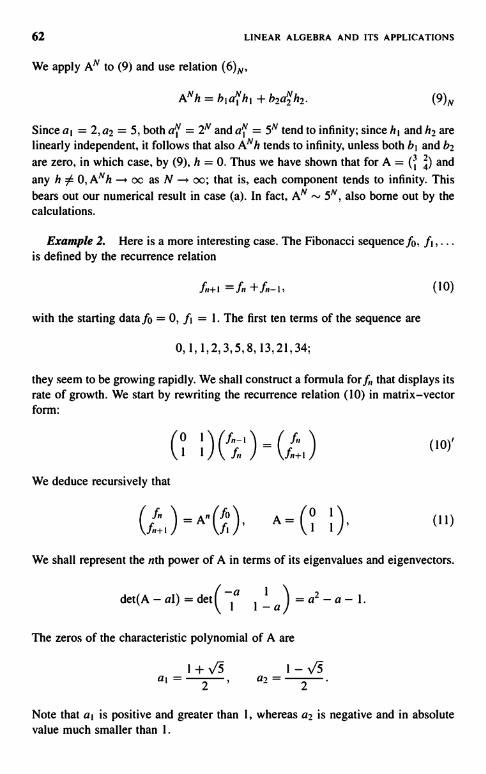
62 LINEAR ALGEBRA AND ITS APPLICATIONS
We apply AN to (9) and use relation (6)N,
ANh = b, a' h, + b2a2 h2. (9)N
Since a, = 2, a2 = 5, both a'' = 2N and 5N tend to infinity; since h, and h2 arelinearly independent, it follows that also ANh tends to infinity, unless both b, and b2are zero, in which case, by (9), h = 0. Thus we have shown that for A = (i 2) andany h ¢ 0, ANh. oc as N - oo; that is, each component tends to infinity. Thisbears out our numerical result in case (a). In fact, AN - 5N, also borne out by thecalculations.
Example 2. Here is a more interesting case. The Fibonacci sequence fo, f,....is defined by the recurrence relation
=fn
with the starting data fo = 0, f, = 1. The first ten terms of the sequence are
0,1,1,2,3,5,8,13,21,34;
(10)
they seem to be growing rapidly. We shall construct a formula for f that displays itsrate of growth. We start by rewriting the recurrence relation (10) in matrix-vectorform:
( I I) (ff, I )
We deduce recursively that
Gf,
fn+i(10)'
(ff+I) = An(f ), A= (0 1), (11)
We shall represent the nth power of A in terms of its eigenvalues and eigenvectors.
det(A - al) = det(la
I I a) = a22 - a - 1.
The zeros of the characteristic polynomial of A are
1+vf5- 1-fa, = 2 a2 = 2
Note that a, is positive and greater than 1, whereas a2 is negative and in absolutevalue much smaller than 1.

SPECTRAL THEORY
The eigenvectors satisfy the equations
a, 1 a2 1
h, = 0, h2 = 0.1 1-a, 1 1-a2
These equations are easily solved by looking at the first component:
h,a,= ( I ) h2 = I a2 I;
63
of course any scalar multiples of them are eienvectors as well.Next we express the initial vector 004 1) _ (0, 1)T as a linear combination of
the eigenvectors:
(?) = c,h1 + CA).
Comparing the first component shows that c2 = -Cl. The second component yieldsc, = 1/f. So
(f' 1 =I h,-7h2.Vr5
Set this into (11); we get
G,+I ) = 75 Vr5- 75-The first component of this vector equation is
f"=ai/v'-az/f.Since a2/F5 is less than 1/2, and since f is an integer, we can put this relation inthe following form:
a"f = nearest integer to
EXERCISE I. Calculate f32.
We return now to the general case (6), (8). The characteristic polynomial of thematrix A,
det(aI - A) = pA(a),
is a polynomial of degree n; the coefficient of the highest power a" is 1.
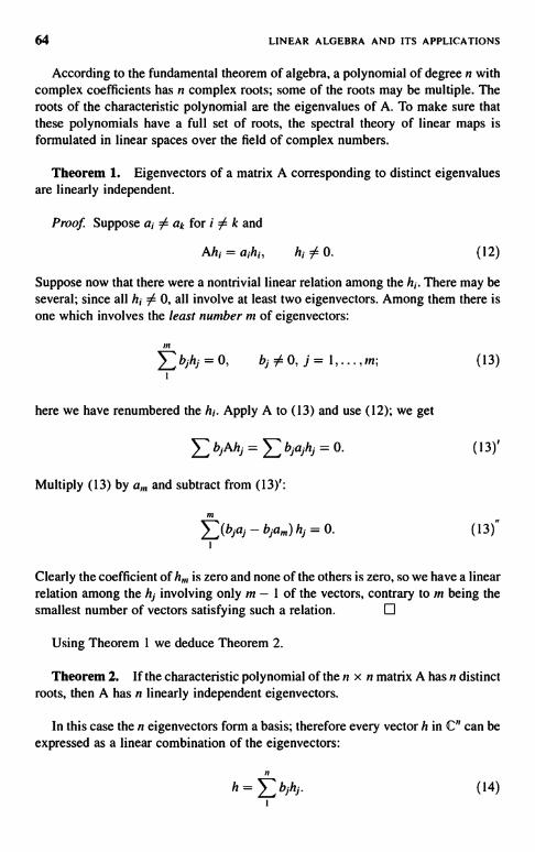
64 LINEAR ALGEBRA AND ITS APPLICATIONS
According to the fundamental theorem of algebra, a polynomial of degree n withcomplex coefficients has n complex roots; some of the roots may be multiple. Theroots of the characteristic polynomial are the eigenvalues of A. To make sure thatthese polynomials have a full set of roots, the spectral theory of linear maps isformulated in linear spaces over the field of complex numbers.
Theorem 1. Eigenvectors of a matrix A corresponding to distinct eigenvaluesare linearly independent.
Proof. Suppose ai # ak for i # k and
Ahi = aihi, hi 0. (12)
Suppose now that there were a nontrivial linear relation among the hi. There may beseveral; since all hi # 0, all involve at least two eigenvectors. Among them there isone which involves the least number m of eigenvectors:
m
bjhh=0, b1#0, j=I...... ; (13)
here we have renumbered the hi. Apply A to (13) and use (12); we get
Eb1Ah,=>bjajhj=0. (13)'
Multiply (13) by aand subtract from (13)':
ni
E(bjaj-bja,n)hh=0. (13)"
Clearly the coefficient of h,,, is zero and none of the others is zero, so we have a linearrelation among the h1 involving only m - I of the vectors, contrary to in being thesmallest number of vectors satisfying such a relation.
Using Theorem I we deduce Theorem 2.
Theorem 2. If the characteristic polynomial of the n x n matrix A has n distinctroots, then A has n linearly independent eigenvectors.
In this case the n eigenvectors form a basis; therefore every vector h in C" can beexpressed as a linear combination of the eigenvectors:
h = > bjhj. (14)

SPECTRAL THEORY
Applying AN to (13) and using (6)N we get
ANh = > bja7h,.
65
(14)'
This formula can be used to answer the stability question raised at the beginning ofthis chapter:
EXERCISE 2. (a) Prove that if A has n distinct eigenvalues a1 and all of them areless than one in absolute value, then all h in C",
ANh_O asN oo,
that is, all components of ANh tend to zero.(b) Prove that if all al are greater than one in absolute value, then for all h # 0,
ANh - oc asN ->oc,
that is, some components of ANh tend to infinity.
There are two simple and useful relations between the eigenvalues of A and thematrix A itself.
Theorem 3. Denote by ai, ... , a,, the eigenvalues of A, with the samemultiplicity they have as roots of the characteristic equation of A. Then
E a; = tr A, H a; = det A. (15)
Proof. We claim that the characteristic polynomial of A has the form
PA (S) = s" - (trA)s"-1 + + (-1)"detA. (15)'
According to elementary algebra, the polynomial PA can be factored as
"PA(s) = fl(s - a;); (16)
1
this shows that the coefficient of s"- 1 in PA is - a;, and the constant term is(-1)"fj al. Comparing this with (15)' gives (15).
To prove (15)', we use first formula (16) in Chapter 5 for the determinant as a sumof products:
s-ail -a12
-alt s - a22PACs) = det(sI - A) = det
-a,,,
= E a(p) H (sSr;, - ai)-
-al"

66 LINEAR ALGEBRA AND ITS APPLICATIONS
Clearly the terms of degree n and n - 1 in s come from the single product of thediagonal elements.
fJ(s - ai,) = s" - (trA) s"-' + -
This identifies the terms of order n and (n - 1) in (15). The term of order zero,PA(0), is det (-A) _ (-1)" det A. This proves (15)' and completes the proof ofTheorem 3.
EXERCISE 3. (a) Verify for the matrices discussed in Examples 1 and 2,
3 24) and (0
1
1(1
that the sum of the eigenvalues equals the trace, and their product is the determinantof the matrix.
Relation (6)N, A"h = a"h, shows that if a is an eigenvalue of A, aN is aneigenvalue of AN. Now let q be any polynomial:
q(s) _
Multiplying (6)N by qN and summing we get
q(A)h = q(a)h.
The following result is called the spectral mapping theorem.
(17)
Theorem 4. (a) Let q be any polynomial, A a square matrix, a an eigenvalue ofA. Then q(a) is an eigenvalue of q(A).
(b) Every eigenvalue of q(A) is of the form q(a), where a is an eigenvalue of A.
Proof. Part (a) is merely a verbalization of relation (17), which shows also that Aand q(A) have h as common eigenvector.
To prove (b), let b denote an eigenvalue of q(A); that means that q(A) - bl is notinvertible. Now factor the polynomial q(s) - b:
q(s) - b = c[I(s - r;).
We may set A in place of s:
q(A) - bl = c [J(A - r;l).

SPECTRAL THEORY 67
By taking b to be an eigenvalue of q(A), the left-hand side is not invertible.Therefore neither is the right-hand side. Since the right-hand side is a product, itfollows that at least one of the factors A - riI is not invertible. That means that somer; is an eigenvalue of A. Since r, is a root of q(s) - b,
q(rj) = b.
This completes the proof of part (b).
If in particular we take q to be the characteristic polynomial PA of A, we concludethat all eigenvalues of PA (A) are zero. In fact a little more is true.
Theorem 5 (Cayley-Hamilton). Every matrix A satisfies its own characteristicequation:
PA (A) = 0. (18)
Proof. If A has distinct eigenvalues, then according to Theorem 2 it has n linearlyindependent eigenvectors hj, j = 1, .... n. Using (4) we apply PA(A):
PA(A)h = E PA(aj)bjhj = E 0 = 0
for all h, proving (18) in this case. For a proof that holds for all matrices we use thefollowing lemma.
Lemma 6. Let P and Q be two polynomials with matrix coefficients
P(s) = E PiSi, Q(s) _ Qks' .
The product PQ = R is then
R(s) _ R,st, R, = > PjQkj+k=r
Suppose that the matrix A commutes with the coefficients of Q; then
P(A)Q(A) = R(A). (19)
The proof is self-evident.We apply Lemma 6 to Q(s) = sI - A and P(s) defined as the matrix of cofactors
of Q(s); that is,
(-1)`+jDjrt(s), (20)
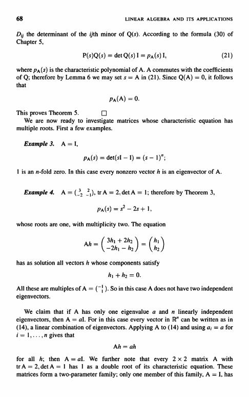
68 LINEAR ALGEBRA AND ITS APPLICATIONS
Dif the determinant of the ijth minor of Q(s). According to the formula (30) ofChapter 5,
P(s)Q(s) = det Q(s) I = pA(s) I, (21)
where pA(s) is the characteristic polynomial of A. A commutes with the coefficientsof Q; therefore by Lemma 6 we may set s = A in (21). Since Q(A) = 0, it followsthat
PA(A) = 0.
This proves Theorem 5.We are now ready to investigate matrices whose characteristic equation has
multiple roots. First a few examples.
Example 3. A = I,
PA(s) = det(sI - I) = (s - 1)";
1 is an n-fold zero. In this case every nonzero vector h is an eigenvector of A.
Example 4. A = (2 z' ), tr A = 2, det A = 1; therefore by Theorem 3,
PA(s) = s2 - 2s + 1,
whose roots are one, with multiplicity two. The equation
Ah = 3hi + 2h-) _ hi
-2h1 - hZ h2
has as solution all vectors h whose components satisfy
hI+h2=0.
All these are multiples of A So in this case A does not have two independenteigenvectors.
We claim that if A has only one eigenvalue a and n linearly independenteigenvectors, then A = aI. For in this case every vector in IB" can be written as in(14), a linear combination of eigenvectors. Applying A to (14) and using a; = a fori = 1,...,n gives that
Ah = ah
for all h; then A = al. We further note that every 2 x 2 matrix A withIT A = 2, det A = I has I as a double root of its characteristic equation. Thesematrices form a two-parameter family; only one member of this family, A = I, has

SPECTRAL THEORY 69
two linearly independent eigenvectors. This shows that, in general, when thecharacteristic equation of A has multiple roots, we cannot expect A to have n linearlyindependent eigenvectors.
To make up for this defect one turns to generalized eigenvectors. In the firstinstance a generalized eigenvectorf is defined as satisfying
(A - aI)2f = 0. (22)
We show first that these behave almost as simply under applications of AN as thegenuine eigenvectors. We set
(A - al) f = h. (23)
Applying (A - aI) to this and using (22), we get
(A - aI)h = 0, (23)'
that is, h is a genuine eigenvector. We rewrite (23) and (23)' as
Af=af+h, Ah=ah. (24)
Applying A to the first equation of (24) and using the second equation gives
A2f = aAf + Ah = a2f + 2ah.
Repeating this N times gives
ANf = aNf + NaN-III. 25)
EXERCISE 4.
EXERCISE 5.
Verify (25) by induction on N.
Prove that for any polynomial q,
q(A)f = q(a)f + q'(a)h, (26)
where q' is the derivative of q and f satisfies (22).
Formula (25) shows that if Ial < 1, and f is a generalized eigenvector of A,ANf -,. 0.
We now generalize the notion of a generalized eigenvector.
Definition. f is a generalized eigenvector of A, with eigenvalue a, if f # 0 and
(A - aI)f =0 (27)
for some positive integer in.We state now one of the principal results of linear algebra.
70 LINEAR ALGEBRA AND ITS APPLICATIONS
Theorem 7 (Spectral Theorem). Let A be an it x it matrix with complexentries. Every vector in C" can be written as a sum of eigenvectors of A, genuine orgeneralized.
For the proof, we need the following results of algebra.
Lemma 8. Let p and q be a pair of polynomials with complex coefficients andassume that p and q have no common zero. Then there are two other polynomials aand b such that
ap + bq - 1. (28)
Proof. Denote by 9 all polynomials of the form ap + bq. Among them there isone, nonzero, of lowest degree; call it d. We claim that d divides both p and q; forsuppose not; then the division algorithm yields a remainder r, say
r = p - md.
Since p and d belong to .f, so does p - and = r; since r has lower degree than d, thisis a contradiction.
We claim that d has degree zero; for if it had degree greater than zero, it would, bythe fundamental theorem of algebra, have a root. Since d divides p and q, this wouldbe a common root of p and q. Since we have assumed the contrary, deg d = 0follows; since d 0 0, d - const., say - 1. This proves (28).
Lemma 9. Let p and q be as in Lemma 8, and let A be a square matrix withcomplex entries. Denote by NN.. Nq, and Npq the null spaces of p(A), q(A), andp(A)q(A), respectively. Then Nnq is the direct sum of NN, and Nq:
Npq=Np®Nq, (29)
by which we mean that every x in Npq can be decomposed uniquely as
x = Xp + xq, xp in Nn, xq in Nq. (29)'
Proof. We replace the argument of the polynomials in (28) by A; we get
a(A)p(A) + b(A)q(A) = I. (30)
Letting both sides act on x we obtain
a(A)p(A)x + b(A)q(A)x = x. (31)
SPECTRAL THEORY 71
We claim that if x belongs to Npq, then the first term on the left in (31) is in Nq, andthe second in Np. To see this we use the commutativity of polynomials of the samematrix:
q(A)a(A)p(A)x = a(A)p(A)q(A)x = 0,
since x belongs to the nullspace of p(A)q(A). This proves that the first term on theleft in (31) belongs to the nullspace of q(A); analogously the second term belongs tothe nullspace of p(A). This shows that (31) gives the desired decomposition (29)'.
To show that the decomposition is unique, we argue as follows: If
x=xp+xq=x'p+xq,
then
y=xp-Xp=a'q-xq
is an element that belongs to both Np and Nq. Let (30) act on y:
a(A)p(A)y + b(A)q(A)y = y.
Both terms on the left-hand side are zero; therefore so is the right-hand side, y. Thisproves that xp = xp, xq = xq.
Corollary 10. Let p,.... ,pk be a collection of polynomials that are pairwisewithout a common zero. Denote the nullspace of the product p, (A) ... pk(A) byNp, ... p,. Then
Np,...p, = Np1 ®... ®NpA. (32)
EXERCISE 6. Prove (32) by induction on k.
Proof of Theorem 7. Let x be any vector; the n + 1 vectors x, Ax, A2x, ... A"xmust be linearly dependent; therefore there is a polynomial p of degree less than orequal to n such that
p(A)x = 0 (33)
We factor p and rewrite this as
fl (A - rjI)m'x = 0. (33)'
72 LINEAR ALGEBRA AND ITS APPLICATIONS
r1 the roots of p, m1 their multiplicity. When r1 is not an eigenvalue of A, A - r1I isinvertible; since the factors in (33)' commute, all invertible factors can be removed.The remaining r1 in (33)' are all eigenvalues of A. Denote
p1(s) = (s - r1)"''; (34)
then (33)' can be written as 11 pp(A)x = 0, that is, x belongs to NN,,...pR. Clearly the p1pairwise have no common zero, so Corollary 10 applies: x can be decomposed as asum of vectors in NPR . But by (34) and Definition (27), every x1 in NN, is a generalizedeigenvector. Thus we have a decomposition of x as a sum of generalizedeigenvectors, as asserted in Theorem 7.
We have shown earlier in Theorem 5, the Cayley-Hamiltonian Theorem, that thecharacteristic polynomial PA of A satisfies pA(A) = 0. We denote by .0='0A the setof all polynomials p which satisfy p(A) = 0. Clearly, the sum of two polynomials in,0 belongs to J; furthermore, if p belongs to J, so does every multiple of p. Denoteby in = mA a nonzero polynomial of smallest degree in J; we claim that all p in Jare multiples of in. Because, if not, then the division process
p = qm + r
gives a remainder r of lower degree than in. Clearly, r = p - qm belongs to 31,contrary to the assumption that in is one of lowest degree. Except for a constantfactor, which we fix so that the leading coefficient Of MA is 1, m = mA is unique. Thispolynomial is called the minimal polynomial of A.
To describe precisely the minimal polynomial we return to the definition (27) of ageneralized eigenvector. We denote by Aim = N(a) the nullspace of (A - al)m.The subspaces N,,, consist of generalized eigenvectors; they are indexedincreasingly, that is,
(35)
Since these are subspaces of a finite-dimensional space, they must be equal from acertain index on. We denote by d = d(a) the smallest such index, that is,
Nd = nd+I = ... (35)'
but
Nd-I 0 Nd; (35)"
d(a) is called the index of the eigenvalue a.

SPECTRAL THEORY
EXERCISE 7. Show that A maps Nd into itself.
73
Theorem 11. Let A be an n x n matrix: denote its distinct eigenvalues bya,,. .., ak, and denote the index of aj by dj. We claim that the minimal polynomialMA is
h
MA(S) = [J(s - ai)d.
EXERCISE 8. Prove Theorem 11.
Let us denote Nd,(aj) by NU); then Theorem 7, the spectral theorem, can beformulated as follows:
C^ = N(') ®N('-) ® ... ®N(k). (36)
The dimension of NU) equals the multiplicity of a1 as the root of the characteristicequation of A. Since our proof of this proposition uses calculus, we postpone it untilTheorem I 1 of Chapter 9.
A maps each subspace N(j) into itself; such subspaces are called invariant underA. We turn now to studying the action of A on each subspace; this action iscompletely described by the dimensions of N1, N2, ... , Nd in the following sense.
Theorem 12. (i) Suppose the pair of matrices A and B are similar in the senseexplained in Chapter 5 [see equation (37)],
A = SBS-',
S some invertible matrix. Then A and B have the same eigenvalues:
(37)
a, = bi,...,ak = bk; (38)
furthermore, the nullspaces
N(aj) = nullspace of (A - a3I)
and
M(aj) = nullspace of (B - a1I)n,
have for all j and m the same dimensions:
dim N,,,(a3) = dim M,,,(aj). (39)
74 LINEAR ALGEBRA AND ITS APPLICATIONS
(ii) Conversely, if A and B have the same eigenvalues, and if condition (39) aboutthe nullspaces having the same dimension is satisfied, then A and B are similar.
Proof. Part (i) is obvious; for if A and B are similar, so are A - al and B - aI,and so is any power of them:
(A - al)"' = S(B - aI)"'S-1. (40)
Since S is a 1-to-1 mapping, the nullspaces of two similar matrices have the samedimension. Relations (39) and in particular (38), follow from the observation.
The converse proposition will be proved in Appendix 15.Theorems 4, 7, and 12 are the basic facts of the spectral theory of matrices. We
wish to point out that the concepts that enter these theorems-eigenvalue,eigenvector, generalized eigenvector, index-remain meaningful for any mappingA of any finite dimensional linear space X over C into itself. The three theoremsremain true in this abstract context and so do the proofs.
The usefulness of spectral theory in an abstract setting is shown in the followingimportant generalization of Theorem 7.
Theorem 14. Denote by X a finite-dimensional linear space over the complexnumbers, by A and B linear maps of X into itself, which commute:
AB = BA. (41)
Then there is a basis in X which consists of eigenvectors and generalizedeigenvectors of both A and B.
Proof. According to the Spectral Theorem, Theorem 7, equation (36), X can bedecomposed as a direct sum of generalized eigenspaces of A:
X=N(W)EB...(B- N(k),
NU) the nullspace of (A - ajI)`t1. We claim that B maps NU) into NU); for B isassumed to commute with A, and therefore commutes with (A - aI)e:
B(A - aI)`tx = (A - aI)"Bx. (42)
If a is an eigenvalue and x belongs to NU), the left-hand side of (42) is 0; therefore sois the right-hand side, which proves that Bx is in NUI. Now we apply the SpectralTheorem to the linear mapping B acting on N(i) and obtain a spectral decompositionof each N(j) with respect to B. This proves Theorem 14.
Corollary 15. Theorem 14 remains true if A, B are replaced by any number ofpairwise commuting linear maps.
SPECTRAL THEORY
EXERCISE 9. Prove Corollary 15.
75
In Chapter 3 we defined the transpose A' of a linear map. When A is a matrix, thatis, a map C" - C", its transpose AT is obtained by interchanging the rows andcolumns of A.
Theorem 16. Every square matrix A is similar to its transpose AT.
Proof We have shown in Chapter 3, Theorem 6, that a mapping A of a space Xinto itself, and its transpose A' mapping X' into itself, have nullspaces of the samedimension. Since the transpose of A - aI is A' - al' it follows that A and A' have thesame eigenvalues, and that their eigenspaces have the same dimension.
The transpose of (A - al)' is (A' - al')'; therefore their nullspaces have the samedimension. We can now appeal to Theorem 12 and conclude that A and A',interpreted as matrices, are similar.
Theorem 17. Let X be a finite-dimensional linear space over C, A a linearmapping of X into X. Denote by X' the dual of X, A': X' -> X' the transpose of A. Leta and b denote two distinct eigenvalues of A: a 54 b, x an eigenvector of A witheigenvalue a, l an eigenvector of A' with eigenvalue b. Then 1 and x annihilate eachother:
(1,x) = 0. (43)
Proof. The transpose of A is defined in equation (9) of Chapter 3 by requiringthat for every x in X and every I in X'
(A'/,x) = (1,Ax).
If in particular we take x to be an eigenvector of A and I to be an eigenvector of A',
Ax = ax, A'1=b1,
and we deduce that
b(l,x) = a(l,x).
Since we have taken a 54 b, (I, x) must be zero.
Theorem 17 is useful in calculating and studying the properties of expansions ofvectors x in terms of eigenvectors.
76 LINEAR ALGEBRA AND ITS APPLICATIONS
Theorem 18. Suppose the mapping A has n distinct eigenvalues a1, ... , a,,.Denote the corresponding eigenvectors of A by x, ...... x,,, those of A' by 11, ...Then
(a)(11,xi)00,i= 1,...,n.(b) Let
x = kjxj.
be the expansion of x as a sum of eigenvectors; then
ki = i = 1,...,n.
EXERCISE 10. Prove Theorem 18.
EXERCISE I I. Take the matrix
(44)
(45)
from equation (10)' of Example 2.
(a) Determine the eigenvector of its transpose.(b) Use formulas (44) and (45) to determine the expansion of the vector (0, 1)'
in terms of the eigenvectors of the original matrix. Show that your answeragrees with the expansion obtained in Example 2.
EXERCISE 12. In Example 1 we have determined the eigenvalues andcorresponding eigenvector of the matrix
C31
2)4
as al =2,h1 = 1 21
Determine eigenvectors 11 and 12 of its transpose and show that
0 fori54 j(fi,hi)=540 fori=j
EXERCISE 13. Show that the matrix
(01A= 0 1
1 1 0
has I as an eigenvalue. What are the other two eigenvalues?
CHAPTER 7
Euclidean Structure
In this chapter we abstract the concept of Euclidean distance. We gain no greatergenerality; we gain simplicity, transparency and flexibility.
We review the basic structure of Euclidean spaces. We choose a point 0 as originin real n-dimensional Euclidean space; the length of any vector x in space, denotedas 11 x 11, is defined as its distance to the origin.
Let us introduce a Cartesian coordinate system and denote the Cartesiancoordinates of x as xi , ... , x,,. By repeated use of the Pythagorean theorem we canexpress the length of x in terms of its Cartesian coordinates.
xx,+ +x.The scalar pmduct of two vectors x and y, denoted as (x, ),), is defined by
(x, y) = > xiyi
(1)
(2)
Clearly, the two concepts are related; we can express the length of a vector as
II x 112 = (X, X). (2)'
The scalar product is commutative:
(x, Y) = (Y' X) (3)
and bilinear:
(x + U, Y) _ (x,y) + (u,y),(3)'
(x,y+v) _ (x,y)+(x,v).
Linear Algebra and Its Applications. Second Edition, by Peter D. LaxCopyright ``.i 2007 John Wiley & Sons, Inc.
77
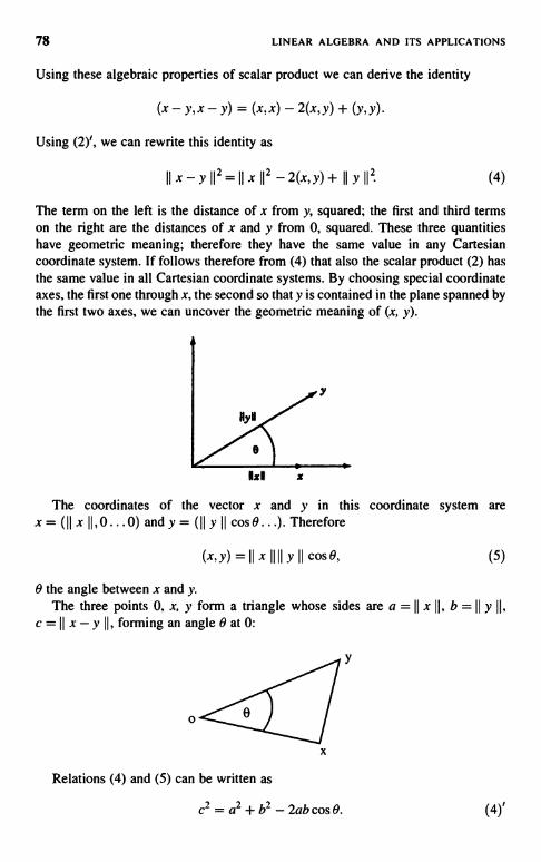
78 LINEAR ALGEBRA AND ITS APPLICATIONS
Using these algebraic properties of scalar product we can derive the identity
(x - y,x - y) = (x,x) - 2(x,y) + ()',Y)
Using (2)', we can rewrite this identity as
IIx-YII2= IIx1I2 -2(x,y)+ IIYII? (4)
The term on the left is the distance of x from y, squared; the first and third termson the right are the distances of x and y from 0, squared. These three quantitieshave geometric meaning; therefore they have the same value in any Cartesiancoordinate system. If follows therefore from (4) that also the scalar product (2) hasthe same value in all Cartesian coordinate systems. By choosing special coordinateaxes, the first one through x, the second so that y is contained in the plane spanned bythe first two axes, we can uncover the geometric meaning of (x, y).
IxI x
The coordinates of the vector x and y in this coordinate system arex = ( I I x 1 1 , 0. .. 0) and y = (II )' II cos 0 ...). Therefore
(x,Y)=IIx1IIIYIIcose, (5)
0 the angle between x and y.The three points 0, x, y form a triangle whose sides are a = II x II, b = II y II,
c=IIx - y 11, forming an angle Oat 0:
Relations (4) and (5) can be written as
c' = a2 + b 2 - 2ab cos 0. (4)'

EUCLIDEAN STRUCTURE 79
This is the classical law of cosine; a special case of it, 0 = n/2, is the Pythagoreantheorem.
Most texts derive formula (5) for the scalar product from the law of cosine. This isa pedagogical blunder, for most students have long forgotten the law of cosine, ifthey ever knew it.
We shall give now an abstract, that is axiomatic, definition of Euclidean space.
Definition. A Euclidean structure in a linear space X over the reals is furnishedby a real-valued function of two vector arguments called a scalar product anddenoted as (x, y), which has the following properties:
(I) (x, y) is a bilinear function; that is, it is a linear function of each argumentwhen the other is kept fixed.
(ii) It is symmetric:
(x, Y) = (Y,x) (6)
(iii) It is positive:
(x,x) > 0 except for x = 0. (7)
Note that the scalar product (2) satisfies these axioms. We shall show now that,conversely, all of Euclidean geometry is contained in these simple axioms.
We define the Euclidean length (also called norm) of x by
IIxII=(x,x)1,2.
(8)
A scalar product is also called an inner product, or a dot product.
Definition. The distance of two vectors x and y in a linear space with Euclideannorm is defined as 11 x - y 11.
Theorem I (Schwarz Inequality). For all x, y,
I(x,Y)I<_IIx1IIIYII. (9)
Proof. Consider the function q(t) of the real variable t defined by
q(t) = II x + ty II? (10)
Using the definition (8) and properties (i) and (ii) we can write
q(t) = 11 x 112 + 2t(x, y) + t2 II Y112. (10),

80 LINEAR ALGEBRA AND ITS APPLICATIONS
Assume that y 96 0 and set t = -(x, y)/ II y 112 in (10)'. Since (10) shows thatq(t) > 0 for all t, we get that
11x112-(x,y)2>0
I1y11
This proves (9). For y = 0, (9) is trivially true.
Note that for the concrete scalar product (2), inequality (9) follows from therepresentation (5) of (x, y) as 11 x 1111 y 11 cos 9.
Theorem 2
11 x 11 = max(x,y), 11yI1=1.
EXERCISE I. Prove Theorem 2.
Theorem 3 (Triangle Inequality). For all x, y
IIx+y11:5 11x11+11y1I. (12)
Proof. Using the algebraic properties of scalar product, we derive, analogously to(4), the identity
11X+y112=11x112+2(x,y)+1Iy112
(12)'
and estimate the middle term by the Schwarz inequality.
Motivated by (5) we make the following definitions.
Definition. Two vectors x and y are called orthogonal (perpendicular), denotedas x .1.. y, if
(x,y) = 0. (13)
From (12)' we deduce the Pythagorian theorem
IIx+y112=11x112+11y112 ifxly. (13)'
Definition. Let X be a finite-dimensional linear space with a Eulerian structure,P), ... , x(") a basis for X. This basis is called orthononnal with respect to a givenEuclidean structure if
(x(i) x(k)) = J 0, for j # k,(14)
1, forj = k.
EUCLIDEAN STRUCTURE 81
Theorem 4 (Gram-Schmidt). Given an arbitrary basis y( 1). ... , y(") in a finite-dimensional linear space equipped with a Euclidean structure, there is a related basisx(1), ..,x(") with the following properties:
(i) x(1),...,x(") is an orthonormal basis.(ii) x(k) is a linear combination of y( I), .. , y(k), for all k.
Proof. We proceed recursively; suppose x(1>, .... x(k-0 have already beenconstructed. We set
k-Ix(k) = C y(k) -
I
Cixtn
Since x(j), . , x(k-1) are already orthonormal, it is easy to see that x(k) defined aboveis orthogonal to them if we choose
cr = (Y(k),x(r>), l = 1,...,k - 1.
Finally we choose c so that 11 x1 11 = 1.
Theorem 4 guarantees the existence of plenty of orthonormal bases. Given such abasis, any x can be written as
X = ajx(j) (15)
Take the scalar product of (15) with x(1); using the orthonormality relations (14) weget
(x, x(')) = at. (16)
Let y be any other vector in X; it can be expressed as
Y = E bkx(k)
Take the scalar product of y with x, using the expression (15). Then, using (14), weget
(x, 3') _ ajbk (x(i) x(k)) _ ajbj. (17)
In particular, for y = x we get
1 1 X =1:a". (17)'
82 LINEAR ALGEBRA AND ITS APPLICATIONS
Equation (17) shows that the mapping defined by (16),
x -> (ai.... ,a"),
carries the space X with a Euclidean structure into R", and carries the scalar productof X into the standard scalar product (2) of R".
Since the scalar product is bilinear, for y fixed (x, y) is a linear function of x.Conversely, we have the following theorem.
Theorem 5. Every linear function l(x) on a finite-dimensional linear space Xwith Euclidean structure can be written in the form
1(x) = (x,y), (18)
y some element of X.
Proof. Introduce an orthonormal basis xi ), ... , x(") in X; denote the value of Ionxik) by
l(x(k)) = bk.
Set y = >bkx(19)It follows from orthonormality that (x(k),y) = bk. This shows that (18) holds forx = xik), k = 1, 2, ... , n; but if two linear functions have the same value for allvectors that form a basis, they have the same value for all vectors X. El
Corollary 5'. The mapping I -+ y is an isomorphism of the Euclidean space Xwith its dual.
Definition. Let X be a finite-dimensional linear space with Euclidean structure,Y a subspace of X. The orthogonal complement of Y, denoted as Y1, consists of allvectors z in X that are orthogonal to every y in Y.
z in Y1 if (y, z) = 0 for all y in Y.
Recall that in Chapter 2 we denoted by Y1 the set of linear functionals that vanishon Y The notation Y1 introduced above is consistent with the previous notation whenthe dual of X is identified with X via (18). In particular, Y' is a subspace of X.
Theorem 6. For any subspace Y of X,
X=YEY1. (20)
EUCLIDEAN STRUCTURE 83
The meaning of (20) is that every x in X can be decomposed uniquely as
x = y + y1, y in Y, .y1 orthogonal to Y. (20)'
Proof. We show first that a decomposition of form (20)' is unique. Suppose wecould write
x = z + z1, zin Y, z1 in Y.
Comparing this with (20)' gives
Y-z=z1- Y.L.
It follows from this that y - z belongs both to Yand to Y1, and thus is orthogonal toitself:
0=(Y-z, z1-y1)=(Y-z,Y-z)=11y-z 112,
but by positivity of norm, y - z = 0.To prove that a decomposition of form (20)' is always possible, we construct an
orthonormal basis of X whose first k members lie in Y; the rest must lie in Y1. We canconstruct such a basis by starting with an orthonormal basis in Y, then complete it to abasis in X, and then orthonormalize the rest of the basis by the procedure describedin Theorem 3. Then x can be decomposed as in (15). We break this decompositioninto two parts:
k
x=>2aixul = +Y+Y1;1 k+1
clearly, y lies in Y and y1 in Y1.
(21)
In the decomposition (20)', the component y is called the orthogonal projection ofx into Y, denoted by
y = Pyx.
Theorem 7. (1) The mapping Py is linear.(ii) p2 = Py.
(22)
Proof Let w be any vector in X, unrelated to x, and let its decomposition (20)' be
w = z + z1, zin Y, z1 in Y1
Adding this to (20)' gives
x+w=(y+z)+ (y1+z1),

84 LINEAR ALGEBRA AND ITS APPLICATIONS
the decomposition of x + w. This shows that Py(x + w) = Pyx + Pyw, Similarly,Py(kx) = kPyx.
To show that Py = Py, we take any x and decompose it as in (20)'; x = y + y'.The vector y = Px needs no further decomposition: Pyy = y.
Theorem 8. Let Y be a linear subspace of the Euclidean space X, x some vectorin X. Then among all elements z of Y, the one closest in Euclidean distance to x isPyx.
Proof. Using the decomposition (20)' of x we have
x-z=y-z+y1, y
Since y and z both belong to Y, so does y - z.Therefore by the Pythagorean theorem (13)',
IIx-Z112 =IIy-ZII2 +IIy1 IIz;
clearly this is smallest when z = y. Since the distance between two vectors x, z is11 x - z 11, this proves Theorem 8.
We turn now to linear mappings of a Euclidean space X into another Euclideanspace U. Since a Euclidean space can be identified in a natural way with its owndual, the transpose of a linear map A of such a space X into U maps U into X. Toindicate this distinction, and for yet another reason explained at the end of thischapter, the transpose of a map A of Euclidean X into U is called the adjoint of A andis denoted by A*.
Here is the full definition of the adjoint A" of a linear mapping A of a Euclideanspace X into another Euclidean space U:
Given any it in U,
1(x) = (Ax, u)
is a linear function of x, According to Theorem 5, this linear function 1(x) can berepresented as (x, y), y in X. Therefore for all x in X
(x, )') = (Ax, u). (23)
The vector y depends on u; Since scalar products are bilinear, y depends linearly onu; we denote this dependence as y = A*u, and rewrite (23) as
(x, A* u) = (Ax, u). (23)'
Note that A" maps U into X; the parentheses on the left denote the scalar product inX, while those on the right denote the scalar product in U.
The next theorem lists the basic properties of adjointness:
EUCLIDEAN STRUCTURE 85
Theorem 9. (i) If A and B are linear mappings of X into U, then
(A+B)'=A`+B'.
(ii) If A is a linear map of X into U, while C is a linear map of U into V, then
(CA)' = A*C*.
(lii) If A is a 1-to-1 mapping of X onto U, then
(A-')* = (A*)-'.
(iv) (A*)* = A.
Proof. (i) is an immediate consequence of (23)'; (ii) can be demonstrated in twosteps:
(CAx, v) _ (Ax, C* v) _ (x, A'C*v).
(iii) follows from (ii) applied to A-' A = 1, 1 the identity mapping, and theobservation that 1` = 1. (iv) follows if we use the symmetry of the scalar product torewrite (23)' as
(u, Ax) = (A*u, x).
When we take X to be R" and U to be 68with their standard Euclidean structures,and interpret A and A* as matrices, they are transposes of each other.
We present now an important application of the notion of the adjoint.There are many situations where quantities x1, ... ,x cannot be measured
directly, but certain linear combinations of them,
can. Suppose that n such linear combinations have been measured. We can put allthis information in the form of a matrix equation
Ax=P, (24)
where p l, ... , p,,, are the measured values, and A is an m x n matrix. We shallexamine the case where the number m of measurements exceeds the number n ofquantities whose value is of interest to us. Such a system of equations isoverdetermined and in general does not have a solution. This is not as alarming as itsounds, because no measurement is perfect, and therefore none of the equations isexpected to hold exactly. In such a situation, we seek that vector x that comes closestto satisfying all the equations in the sense that makes II Ax - P 112 as small aspossible.
86 LINEAR ALGEBRA AND ITS APPLICATIONS
For such an x to be determined uniquely, A cannot have nonzero nullvectors. Forif Ay = 0, and x a minimizer of II Ax - p II, then so is x + ky, k any number.
Theorem 10. Let A be an m x n matrix, m > n, and suppose that A has only thetrivial nullvector 0. The vector x that minimizes II Ax - p 112 is the solution z of
A*Az = A*p. (25)
Proof. We show first that equation (25) has a unique solution. Since the range ofA* is 118", (25) is a system of n equations for n unknowns. According to Corollary Bin Chapter 3, a unique solution is guaranteed if the homogeneous equation
A*Ay = 0 (25)'
has only the trivial solution y = 0. To see that this is the case, take the scalar productof (25)' with y. We get, using the definition (23)' of adjointness, 0 = (A*Ay,y) =(Ay, Ay) =11 Ay 112. Since 11 11 is positive, it follows that Ay = 0. Since we haveassumed that A has only the trivial nullspace, y = 0 follows.
A maps 08" into an n-dimensional subspace of 08"'. Suppose z is a vector in U8"with the following property:
Az - p is orthogonal to the range of A. We claim that such a z minimizesII Ax - p 112. To see this let x be any vector in 08"; split it as x = z + y; then
Ax - p = A(z + y) - p = Az - p + Ay.
By hypothesis Az - p and Ay are orthogonal; therefore by the Pythagoreantheorem,
IIAx -p1I2=IIAz-pII2+IIAy II2.
this demonstrates the minimizing property of z.To find z, we write the condition imposed on z in the form
(Az - p, Ay) = 0 for all y.
Using the adjoint of A we can rewrite this as
(A* (Az - p), y) = 0 for all Y.
The range of A* is 118", so for this condition to hold for all y, A*(Az - p) must be 0,which is equation (25) for z.
Theorem 11. An orthogonal projection Py defined in equation (22) is its ownadjoint,
Py = Py.

EUCLIDEAN STRUCTURE 87
EXERCISE 2. Prove Theorem 11.
We turn now to the following question: what mappings M of a Euclidean spaceinto itself preserve the distance of any pair of points, that is, satisfy for all x, y,
II M(x)-M(y) II=IIx - Y II ? (26)
Such a mapping is called an isomnetry. It is obvious from the definition that thecomposite of two isometries is an isometry. An elementary example of an isometry istranslation:
M(x)=x+a,
a some fixed vector. Given any isometry, one can compose it with a translation andproduce an isometry that maps zero to zero. Conversely, any isometry is thecomposite of one that maps zero to zero and a translation.
Theorem 12. Let M be an isometric mapping of a Euclidean space into itselfthat maps zero to zero:
M(O) = 0. (27)
(i) M is linear.
(ii) M*M=I. (28)
Conversely, if (28) is satisfied, M is an isometry.(iii) M is invertible and its inverse is an isometry.(iv) det M = ±1.
Proof. It follows from (26) with y = 0 and (27) that
IIM(x)II=IIxII
Now let us abbreviate the action of M by':
M(x) = a', M(y) = y'.
By (29),
IIxII=IIxII, IIy 11=IIxII
By (26),
(29)
(29)'
11 x'-y 11=11X-Y11.

88 LINEAR ALGEBRA AND ITS APPLICATIONS
Square and use expansion (4) on both sides:
II x' 112-2(x,y)+IIy 112=11x112-2(x,Y)+IIY112.
Using (29)', we conclude that
(x',)') = (X, Y);
that is, M preserves the scalar product.Let z be any other vector, z' = M(z); then, using (4) twice we get
Ilz' - X, - .v'112 =11z'1I2+11Y'112+IIx 112
-2(z',x) -2(z',.v)+2(x',)1).
Similarly,
IIz-x-Y112=11zII2+IIY112+IIx112-2(z,x)-2(z,y)+2(x,y).
Using (29)' and (30) we deduce that
II z'-x'-Y' 112=11 z - x - Y 112
(30)
We choose now z = x + y; then the right-hand side above is zero; therefore so is11
z' - x' - y' 112. By positive definiteness of the norm z' - x' - y = 0. This provespart (i) of Theorem 12.
To prove part (ii), we take relation (30) and use the adjointness identity (23)':
(Mx, My) = (x, M*My) = (x, y)
for all x and y, so
(x, M*My - Y) = 0.
Since this holds for all x, it follows that M*My - y is orthogonal to itself, and so, bypositiveness of norm, that for all y,
M*My-y=0.
The converse follows by reversing the steps: this proves part (ii).It follows from (29) that the nullspace of M consists of the zero vector; it follows
then from Corollary (B)' of Chapter 3 that M is invertible. That M- 1 is an isometry isobvious. This proves (iii).
It was pointed out in equation (33) of Chapter 5 that for every matrix det M* _det M; it follows from (28) and the product rule for determinants [see (18)in Chapter 5] that (det M)2 = det I = 1, which implies that
detM=f1. (31)
This proves part (iv) of Theorem 12.

EUCLIDEAN STRUCTURE 89
The geometric meaning of (iv) is that a mapping that preserves distances alsopreserves volume.
Definition. A matrix that maps R" onto itself isometrically is called orthogonal.
The orthogonal matrices of a given order form a group under matrixmultiplication. Clearly, composites of isometries are isometric, and so, by part(iii) of Theorem 12, are their inverses.
The orthogonal matrices whose determinant is plus 1 form a subgroup, called thespecial orthogonal group. Examples of orthogonal matrices with determinant plus Iin three-dimensional space are rotations; see Chapter 11.
EXERCISE 3. Construct the matrix representing reflection of points in 1183 acrossthe plane X3 = 0. Show that the determinant of this matrix is -1.
EXERCISE 4. Let R be reflection across any plane in R3.
(1) Show that R is an isometry.(ii) Show that R2 = I.(iii) Show that R* = R.
We recall from Chapter 4 that the ijth entry of the matrix product AB is the scalarproduct of the ith row of A with the jth column of B. The ith row of M* is thetranspose of the ith column of M. Therefore the identity M*M = I characterizingorthogonal matrices can be formulated as follows:
Corollary 12'. A matrix M is orthogonal iff its columns are pairwise orthogonalunit vectors.
EXERCISE 5. Show that a matrix M is orthogonal iff its rows are pairwiseorthogonal unit vectors.
How can we measure the size of a linear mapping A of one Euclidean space X intoanother Euclidean space U? Recall from a rigorous course on the foundations ofcalculus the concept of least upper bound, also called supremum, of a bounded set ofreal numbers, abbreviated as sup. Each component of Ax is a linear function of thecomponents of x; II Ax II2 is a quadratic function of the components of x, andtherefore the set of numbers II Ax II2, II X II2 = 1 is a bounded set.
Definition
II A 11= sup II Ax II (32)16x11=I
Note that 11 Ax 11 is measured in U, 11 x 11 in X. 11 A 11 is called the nonn of A.
90 LINEAR ALGEBRA AND ITS APPLICATIONS
Theorem 13. Let A be a linear mapping from the Euclidean space X into theEuclidean space U, where II A 11 is its norm.
(i)IIAzII:5 IIA1111zII for all z in X. (33)
II A 11= sup (Ax, v). (34)
Proof. (i) follows for unit vectors z from the definition (32) of II A 11. For anyz 0 0, write z = kx,x a unit vector; since II Akx II = II kAx II = kill Ax 11 and
11 kx 11= IkI 11 x 11, (33) follows. For z = 0, (33) is obviously true.(ii) According to Theorem 2,
11u11=max(u,v), 11v11=1.
Set Ax = u in definition (32), and we obtain (34).
EXERCISE 6. Show that Iail < 11 A 11
Theorem 14. For A as in Theorem 13, we have the following:
(i) II kA II = IkI II A II for any scalark.
(ii) For any pair of linear mappings A and B of X into U,
11A+Bll<IIA11+11B11. (35)
(iii) Let A be a linear mapping of X into U, and let C be a linear mapping of Uinto V; then
IICA II<_IICIIIIAII. (36)
IIA 11=11 All.
Proof. (i) follows from the observation that 11 kAx 11= lkl 11 Ax 11.(ii) By the triangle inequality (12), for all x in X we obtain
(37)
II (A + B)x 11=11 Ax + Bx 11 <11 Ax 11 + 11 Bx 11.
EUCLIDEAN STRUCTURE 91
The supremum of the left-hand side for II x II = I is II A + B II. The right-hand sideis a sum of two terms; the supremum of the sum is < the sum of the suprema, whichis IIAII+IIBII-
(iii) By inequality (33),
IIcAxII<-IICIIIIAx 1I.
Combined with (33), this yields
IICAxiI<_IICIIIIAIIIIxiI
Taking the supremum for all unit vectors x gives (36).(iv) According to (23)',
(Ax,v) = (x,A"v);
since the scalar product is a symmetric function, we obtain
(Ax, v) = (A*v,x).
Take the supremum of both sides for all x and v, II x II = 1, II v II = 1. According to(34), on the left-hand side we get II A II, and on the right-hand side we obtainIIA*II. o
The following result is enormously useful:
Theorem 15. Let A be a linear mapping of a finite-dimensional Euclideanspace X into itself that is invertible. Denote by B another linear mapping of X into Xclose to A in the sense of the following inequality:
IIA - B II<1/IIA-' II. (38)
Then B is invertible.
Proof. Denote A - B = C, so that B = A - C. Factor B as
B = A(I - A-'C) = A(I - S),
where S = A-'C.We have seen in Chapter 3 that the product of invertible maps is invertible;
therefore it suffices to show that I - S is invertible. We see that it suffices to showthat the nullspace of 1- S is trivial. Suppose not; that is, (I - S)x = 0, x # 0. Thenx = Sx; using the definition of the norm of S,
IIx1I=II Sxii<_II S IIIIxII.
92
Since x 54 0, it follows that
LINEAR ALGEBRA AND ITS APPLICATIONS
1<_IISI1 (39)
But according to part (iii) of Theorem 14,
IIS11=11A-'CII:5 IIA-' II11c11<1,
where in the last step we have used inequality (38): 11 C II < I / II A II -' Thiscontradicts (39). O
Note. In this proof we have used the finite dimensionality of X. A proof ofTheorem 15 given in Chapter 15 is valid for infinite-dimensional X.
We recall now another concept from a rigorous calculus course:Convergence. A sequence of numbers {ak} tends to a,
lim ak = a,
if lak - al tends to zero. Recall furthermore the notion of a Cauchy sequence ofnumbers {ak}; it is a sequence for which lak - ail tends to zero as j and k tend to oo.A basic property of real numbers is that every Cauchy sequence of numbersconverges to a limit.
This property of real numbers is called completeness.A second basic notion about real numbers is local compactness: Every bounded
sequence of real numbers contains a convergent subsequence.We now show how to extend these notions and results from numbers to vectors in
a finite-dimensional Euclidean space.
Definition. A sequence of vectors {xk} in a linear space X with Euclideanstructure converges to the limit x:
lim xk = xkx
if 11 xk - x II tends to zero as k -> oo.
Theorem 16. A sequence of vectors {xk} in a Euclidean space X is called aCauchy sequence if II xk - xj II -> 0 as k and j -> oo.
(i) Every Cauchy sequence in a finite-dimensional Euclidean space converges toa limit.
A sequence of vectors {Xk } in a Euclidean space X is called bounded if 11 xk 11:5 Rfor all k, R some real number.
(ii) In a finite-dimensional Euclidean space every bounded sequence contains aconvergent subsequence.
EUCLIDEAN STRUCTURE 93
Proof. (i) Let x and y be two vectors in X, a1 and bj their jth component; then
Ia! - bbl <- IIx - yII.
Denote by ak,j thejth component of xk. Since {xk} is a Cauchy sequence, it followsthat the sequence of numbers {akj} also is a Cauchy sequence. Since the realnumbers are complete, the {akr } converge to a limit a1. Denote by x the vector whosecomponents are (a 1, . . . , a,,). From the definition of Euclidean norm,
a
11xk-x1121ak.j -ai12, (40)
it follows that lim xk = x.(ii) Since lat. I < 11 xk 11, it follows that IakiI < R for all k. Because the real
numbers are locally compact, a subsequence of (a*, I) converges to a limit ai.This subsequences of k - s contains a further subsubsequence such that {ak.2}
converges to a limit a2. Proceeding in this fashion we can construct a subsequence of{xk} for which all sequences {akj}, converge to a limit aa.l.... , n, where n is thedimension of X. Denote by x the vector whose components are From(40) we deduce that the subsequence of {xk} converges to x.
It follows from part (ii) of Theorem 16 that the supremum in the definition (32) of
II A 11 is a maximum:
IIAII=Imax 11 Ax 11. (32)'
It follows from the definition of supremum that II A II cannot be replaced by anysmaller number that is an upper bound of II Ax 11, II x II = 1. It follows that there is asequence of unit vectors {xk}, 11 xk 11= 1, such that
slim 11AxLI1=IIAII
According to Theorem 16, this sequence has a subsequence that converges to a limitx. This vector x maximizes 11 Az 11 for all unit vectors z.
Part (ii) of Theorem 16 has a converse:
Theorem 17. Let X be a linear space with a Euclidean structure, and supposethat it is locally compact-that is, that every bounded sequence {xk} of vectors in Xhas a convergent subsequence. Then X is finite dimensional.
Proof. We shall show that if X is not finite dimensional, then it is not locallycompact. Not being finite dimensional means that given any linearly independent setof vectors yI, ... yk, there is a vectoryk+i that is not a linear combination of them. Inthis way we obtain an infinite sequence of vectors yi,y2, ... such that every finite set
94 LINEAR ALGEBRA AND ITS APPLICATIONS
{y1, ... , yk } is linearly independent. According to Theorem 4, we can apply theGram-Schmidt process to construct pairwise orthogonal unit vectors {x1, ... xk},which are linear combinations of yi, ... , yk. For this infinite sequence
II xk -xj II2=II xk II2 -2(xk,xj)+ II xj II'= 2
for all k j. Therefore this sequence, which is bounded, contains no convergentsubsequence. 0
Theorem 17 is a very useful, and therefore important criterion for a Euclideanspace to be finite dimensional. In Chapter 14 we shall show how to extend it to allnormed linear spaces.
In Appendix 12 we shall give an interesting application.
Definition. A sequence {A"} of mappings converges to a limit A if
lim II A,, -All=0.
EXERCISE 7. Show that {A} converges to A iff for all x, A,,x converges to Ax.
Note. The result in Exercise 7 does not hold in infinite-dimensional spaces.We conclude this chapter by a brief discussion of complex Euclidean structure. In
the concrete definition of complex Euclidean space, definition (2) of the scalarproduct in R" has to be replaced in C" by
(x, y) = E xiy;, (41)
where the bar-denotes the complex conjugate. The definition of the adjoins of amatrix is as in (23)', but in the complex case has a slightly different interpretation.Writing
A = (aj), (Ax); a,jxj
and using the (41) definition of scalar product we can write
(Ax, u) ayxj) u,.i j
This can be rewritten as
xj (raijul)
which shows that (Ax, u) = (x, A"u), where
(A*u)j = aFjute
EUCLIDEAN STRUCTURE 95
that is, the adjoint A` of the matrix A is the complex conjugate of the transpose of A.We now define the abstract notion of a complex Euclidean space.
Definition. A complex Euclidean structure in a linear space X over the complexnumbers is furnished by a complex valued function of two vector arguments, called ascalar product and denoted as (x, y), with these properties:
(i) (x, y) is a linear function of x for y fixed.(ii) Conjugate symmetry: for all x, y,
(x,Y) = (Y,x) (42)
Note that conjugate symmetry implies that (x, x) is real for all x.(iii) Positivity:
(x, x) > 0 for all x 36 0.
The theory of complex Euclidean spaces is analogous to that for real ones, with a fewchanges where necessary. For example, it follows from (i) and (ii) that for x fixed,(x, y) is a skew linear function of y, that is, additive in y and satisfying for anycomplex number k,
(x, ky) = k(x, y). (43)
Instead of repeating the theory, we indicate those places where a slight change isneeded. In the complex case identity (12)' is
IIx+Y 112=11x112+(x,y)+(y,x)+IIY 112
=11 x 112 + 2Re(x, ),) + 11 Y 112, (44)
where Re k denotes the real part of the complex number k.
EXERCISE 8. Prove the Schwarz inequality for complex linear spaces with aEuclidean structure.
EXERCISE 9. Prove the complex analogues of Theorems 6, 7, and 8.
We define the adjoint A* of a linear map A of an abstract complex Euclideanspace into itself by relation (23)' as before:
(x,A*u) = (Ax, u).
EXERCISE 10. Prove the complex analogue of Theorem 9.

96 LINEAR ALGEBRA AND ITS APPLICATIONS
We define isometric maps of a complex Euclidean space as in the real case:
II Mx II=IIxII
Definition. A linear map of a complex Euclidean space into itself that isisometric is called unitary.
EXERCISE 11. Show that a unitary map M satisfies the relations
M"M = 1
and, conversely, that every map M that satisfies (45) is unitary.
EXERCISE 12. Show that if M is unitary, so is M- 1 and M*.
(45)
EXERCISE 13. Show that the unitary maps form a group under multiplication.
EXERCISE 14. Show that for a unitary map M, Idet MI = I.
EXERCISE 15. Let X be the space of continuous complex-valued functions on[-1, 1] and define the scalar product in X by
(f,g) = ff(s)(s)ds.I
Let m(s) be a continuous function of absolute value 1: Im(s) I = 1, -1 < s < 1.Define M to be multiplication by m:
(Mf)(s) = m(s)f(s).
Show that M is unitary.
We give now a simple but useful lower bound for the norm of a matrix mapping acomplex Euclidean space X into itself. The definition of the norm of such a matrix isthe same as in the real case, given by equation (32)':
IIAII=II`"Iax1IAxII
Let A be any square matrix with complex entries, h one of its eigenvectors,chosen to have length 1, and a the eigenvalue:
Ah = ah, 1 1h1 .
Then
IIAh1I=IIah1I=Ial.

EUCLIDEAN STRUCTURE 97
Since II A II is the maximum of II Ax II for all unit vectors x, it follows thatII A II > Ial. This is true for every eigenvalue; therefore
IIAII?maxIa;I, (46)
where the a; range over all eigenvalues of A.
Definition. The spectral radius r(A) of a linear mapping A of a linear spaceinto itself is
r(A) = max I ail , (47)
where the aj range over all eigenvalues of A. So (46) can be restated as follows:
11 All >_ r(A). (48)
Recall that the eigenvalues of the powers of A are the powers of the eigenvaluesof A:
Ajh = A.
Applying (48) to Ai, we conclude that
II AN II > r(AY.
Taking the jth root gives
II AiII'li > r(A)-
Theorem 18. As j tends to oc, (48)j tends to be an equality; that is,
lim II AN 11 0 = r(A).i-x
(48)j
A proof will be furnished in Appendix 10.We shall give now a simple and useful upper bound for the norm of a real m x n
matrix
A = (aj),
mapping R' into R'. For any x in R', set Ax = y, y in R'. The components of y areexpressed in terms of the components of x as follows:
Yi = L agxj.
98 LINEAR ALGEBRA AND ITS APPLICATIONS
Estimate the right-hand side using the Schwarz inequality:
yz =(auxi)< (>a)(xi2).
adding all these inequalities, i = 1,.. . , m, we get
2 zy2 < aMUsing the definition of norm in Euclidean space [see equation (1)], we can rewriteinequality (49) as
11y112_< (sat.) Ilxll',i
Take the square root of this inequality; since y = Ax, we can write it as
1 /2
Ax11<(Ea) Ilxll
The definition of the norm A 11 of the matrix A is
It follows from (50) that
sup 11 Ax 11, I1x11=1.
I/2
IIAII a)
this is the upper bound for A II we set out to prove.
) 1/2
EXERCISE 16. Prove the following analogue of (51) for matrices with complexentries:
iJ
EXERCISE 17. Show that
(49)
(50)
(51)
(51)'
E Iai12 = trAA'. (52)ij

EUCLIDEAN STRUCTURE
EXERCISE 18. Show that
trAA* = tr A* A.
99
EXERCISE 19. Find an upper bound and a lower bound for the norm of the 2 x 2matrix
The quantity (F_ IagI2)I12 is called the Hilbert-Schmidt norm of the matrix A.
Let T denote a 3 x 3 matrix, its columns x, y, and z:
T = (x, y, z).
The determinant of T is, for x and y fixed, a linear function of z:
det (x, y, z) = 1(z). (53)
According to Theorem 5, every linear function can be represented as a scalarproduct:
1(z) = (IV, Z),
where w is some vector depending on x and y:
w = w(x,Y)
(54)
Combining (53) and (54) gives
det (x, y, z) = (w(x, y), z). (55)
We formulate the properties of the dependence of w on x and y as a series of
exercises:
EXERCISE 20. (i) w is a bilinear function of x and y. Therefore we write w as aproduct of x and y, denoted as
w=xxy,
and called the cross product.(ii) Show that the cross product is antisymmetric:
yxx= -xXy.
100 LINEAR ALGEBRA AND ITS APPLICATIONS
(iii) Show that x x y is orthogonal to both x and y.(iv) Let R be a rotation in R3; show that
(Rx) x (Ry) = R(x x y).
(v) Show that
11xx3'11=±11x1111y11sin0,
where 8 is the angle between x and )'.(vi) Show that
1 0 00 x 1 = 00 0 1
(vii) Using Exercise 16 in Chapter 5, show that
fa d bf - ceb x e J = cd - afc f ae - bd
EXERCISE 2I. Show that in a Euclidean space every pair of vector satisfies
11u+vIII +11u-v112=211u1122+211v1I2 (56)

CHAPTER 8
Spectral Theory of Self-AdjointMappings of a Euclidean Spaceinto Itself
In this chapter we shall study mappings A of Euclidean spaces into themselves thatare self-adjoint-that is, are their own adjoints:
A* = A.
When A acts on a real Euclidean space, any matrix representing it in an orthonormalsystem of coordinates is symmetric, that is,
Aij = Aji.
Such mappings are therefore also called symmetric. When A acts on a complexEuclidean space, its matrix representations are conjugate symmetric;
Aij = Aji.
Such mappings are also called Hennitean. We saw in Theorem I 1 of Chapter 7 thatorthogonal projections are self-adjoint. Below we describe another large class ofself-adjoint matrices. In Chapter 11 we shall see that matrices that describe themotion of mechanical systems are self-adjoint.
Definition. Let M be an arbitrary linear mapping in a Euclidean space, Wedefine its self-adjoint part as
M+MsM = (1)2
Linear Algebra and Its Applications. Second Edition, by Peter D. LaxCopyright c'! 2007 John Wiley & Sons, Inc.
101

102
EXERCISE I. Show that
Re (x, Mx) = (x, M,.x). (2)
Let (xi, ... , f (x) be a real-valued twice-differentiable function of n realvariables x1,. .. ,x,, written as a single vector variable x. The Taylor approximationto f at a up to second order reads
f(a + y) = f (a) + 1(y) + 2 q(y) + I IyI I2e(I Iy1I),
where e(d) denotes some function that tends to 0 as d 0,1(y) is a linear function ofy, and q(y) is a quadratic function. A linear function has the form (see Theorem 5 ofChapter 7)
1(y) = (y, g); (4)
LINEAR ALGEBRA AND ITS APPLICATIONS
(3)
g is the gradient off at a; according to Taylor's theorem
ofgi=ax
a=a
(5)
The quadratic function q has the form
q(y) = hiiyiyi.i.i
The matrix (hi) is called the Hessian H off; according to Taylor's theorem,
a2hii = .l
311(j ax; r=a
(6)
(7)
Employing matrix notation and the Euclidean scalar product, we can write q, givenby (4), in the form
q(y) = (y, Hy). (8)
The matrix H is self-adjoint, that is, H* = H :
hi = hi;; (9)
this follows from definition (5), and the fact that the mixed partials of a twice-differentiable function are equal.
Suppose now that a is a critical point of the function f, that is where grad f = gis zero. Around such a point Taylor's formula (3) shows that the behavior off isgoverned by the quadratic term. Now the behavior of functions near critical points
SPECTRAL THEORY OF SELF-ADJOINT MAPPINGS OF A EUCLIDEAN SPACE 103
is of fundamental importance for dynamical systems, as well as in geometry; this iswhat gives quadratic functions such an important place in mathematics and makesthe analysis of symmetric matrices such a central topic in linear algebra.
To study a quadratic function it is often useful to introduce new variables:
Ly = z, (10)
where L, is some invertible matrix, in terms of which q has a simpler form.
Theorem 1. (a) Given a real quadratic form (6) it is possible to changevariables as in (10) so that in terms of the new variables, z, q is diagonal, that is, ofthe form
n
q(L- ' z) _ d; ?.
(b) There are many ways to introduce new variables which diagonalize q;however, the number of positive, negative, and zero-diagonal terms d; appearing in(11) is the same in all of them.
Proof. Part (a) is entirely elementary and constructive. Suppose that one of thediagonal elements of q is nonzero, say h # 0. We then group together all termscontaining y,:
n n
q(y) = h, iy2l + hi;yly; + h;;y;yi.
Since H is symmetric, h;, = hid; so we can write q as
12 1z
hn(YI
+ h,-,' h,;y; f --hi > hIJ)y) .
2 2
Set
We can then write
n
yi+hii h11y1=zi.2
q(y) = huzi + q2 (Y),
(12)
(13)
where q2 depends only on y2,...,y,,.
If all diagonal terms of q are zero but there is some nonzero off-diagonal term, sayh12 = h21 # 0, then we introduce yl + y2 and y, - y2 as new variables, which

104 LINEAR ALGEBRA AND ITS APPLICATIONS
produces a nonzero diagonal term. If all diagonal and off-diagonal terms are zero,then q(y) __ 0 and there is nothing to prove.
We now apply induction on the number of variables n; using (13) shows that if thequadratic function q2 in (n - 1) variables can be written in form (11), then so can qitself. Since y2, ... , y,, are related by an invertible matrix to Z2, , z,,, it followsfrom (12) that the full set y is related to z by an invertible matrix.
EXERCISE 2. We have described above an algorithm for diagonalizing q;implement it as a computer program.
We turn now to part (b); denote by p+, p_, and po the number of terms in (11) thatare positive, negative, and zero, respectively. We shall look at the behavior of q onsubspaces S of li". We say that q is positive on the subspace S if
q(u) > 0 for every u in S, u 0 0. (14)
Lemma 2. The dimension of the largest subspace of 18" on which q is positiveis p+:
q positive on S.p+ = max dim S.
Similarly,
(15)
p_ = max dim S, q negative on S. (15)'
Proof. We shall use representation (11) for q in terms of the coordinateszi. . . . . z ; suppose we label them so that d1,.. . , do are positive, p = p+, the restnonpositive. Define the subspace S+ to consist of all vectors for whichz,,+i = = Zn = 0. Clearly dim S+ = p+, and equally clearly, q is positive onS+. This proves that p+ is less than or equal to the right-hand side of (15). We claimthat the equality holds. Let S be any subspace whose dimension exceeds pi.For any vector u in S, define P. as the vector whose p4 components are the same asthe first p+ components of u, and the rest of the components are zero. Thedimension p+ of the target space of this map is smaller than the dimension of thedomain space S. Therefore, according to Corollary A of Theorem 2, Chapter 3,there is a nonzero vectory in the nullspace of P. By definition of P, the first p+ of thez-components of this vectory are zero. But then it follows from (11) that q(y) < 0;this shows that q is not positive on S. This proves (15); the proof of (15)' isanalogous.
Lemma 2 shows that the numbers p_ and p+ can be defined in terms of thequadratic form q itself, intrinsically, and are therefore independent of the specialchoice of variables that puts q in form (11). Since p+ + p_ + po = it, this proves part(b) of Theorem 1.
SPECTRAL THEORY OF SELF-ADJOINT MAPPINGS OF A EUCLIDEAN SPACE 105
Part (b) of Theorem I is called the law of inertia.
EXERCISE 3. Prove that
p+ + po = max dim S, q > 0 on S
and
p_ + po = max dim S, q < 0 on S.
Using form (6) of q we can reinterpret Theorem 1 in matrix terms. It is convenientfor this purpose to express yin terms of z, rather than the other way around as in (10).So we multiply (10) by L- 1, obtaining
y = Mz, (16)
where M abbreviates L-'. Setting (16) into (8) gives, using the adjoint of M,
q(y) = (y, Hy) = (Mz, HMz) = (z, M"HMz). (17)
Clearly, q in terms of z is of form (11) iff M*HM is a diagonal matrix. So part (a) ofTheorem I can be put in the following form:
Theorem 3. Given any real self-adjoint matrix H, there is a real invertiblematrix M such that
M*HM = D, (18)
D a diagonal matrix.
For many applications it is of utmost importance to change variables so that theEuclidean length of the old and the new variables is the same:
IIy112=IIz11?
For the matrix M in (16) this means that M is an isometry. According to (28) ofChapter 7, this is the case iff M is orthogonal, that is, satisfies
M*M = I. (19)
It is one of the basic theorems of linear algebra, nay, of mathematics itself, that givena real-valued quadratic form q, it is possible to diagonalize it by an isometric changeof variables. In matrix language, given a real symmetric matrix H, there is a realinvertible matrix M such that both (18) and (19) hold.
We shall give two proofs of this important result. The first is based on the spectraltheory of general matrices presented in Chapter 6, specialized to self-adjointmappings in complex Euclidean space.

106 LINEAR ALGEBRA AND ITS APPLICATIONS
We recall from Chapter 7 that the adjoins H* of a linear map H of a complexEuclidean space X into itself is defined by requiring that
(Hx,y) = (x, H*y) (20)
hold for all pairs of vectors x,y. Here the bracket (,) is the conjugate-symmetricscalar product introducd at the end of Chapter 7. A linear map H is calledself-adjoins if
H" = H.
For H self-adjoint, (20) becomes
(Hx,y) = (x, Hy). (20)'
Theorem 4. A self-adjoint map H of complex Euclidean space X into itself hasreal eigenvalues and a set of eigenvectors that form an orthonormal basis of X.
Proof. According to the principal result of spectral theory, Theorem 7 of Chapter6, the eigenvectors and generalized eigenvectors of H span X. To deduce Theorem 4from Theorem 7, we have to show that a self-adjoint mapping H has the followingadditional properties:
(a) H has only real eigenvalues.(b) H has no generalized eigenvectors, only genuine ones.(c) Eigenvectors of H corresponding to different eigenvalues are orthogonal.
(a) If a + ib is an eigenvalue of H, then ib is an eigenvalue of H - al, also self-adjoint. Therefore, it suffices to show that a self-adjoint H cannot have a purelyimaginary eigenvalue ib. Suppose it did, with eigenvector z:
Hz = ibz.
Take the scalar product of both sides with z:
(Hz, z) = (ibz, z) = ib(z, z).
Setting both x and y equal to z in (20)', we get
(Hz, z) _ (z, Hz).
(21)
(21)'
Since the scalar product is conjugate symmetric, we conclude that the two sides of(21)' are conjugates. Since they are equal, the left-hand side of (21) is real. Therefore

SPECTRAL THEORY OF SELF-ADJOINT MAPPINGS OF A EUCLIDEAN SPACE 107
so is the right-hand side; since (z, z) is positive, this can be only if b = 0, as assertedin (a).
(b) A generalized eigenvector z satisfies
Hdz = 0; (22)
here we have taken the eigenvalue to be zero, by replacing H with H - al. We wantto show that then z is a genuine eigenvector:
Hz = 0. (22)'
We take first the case d = 2:
H2z = 0; (23)
we take the scalar product of both sides with z:
(H 2Z, z) = 0. (23)'
Using (20)' with x = Hz, y = z, we get
(H 2Z, z) = (Hz, Hz) = II Hz 112;
using (23)', we conclude that II Hz II = 0, which, by positivity, holds only whenHz=0.
We do now an induction on d; we rewrite (22) as
H2Hd-2z = 0.
Abbreviating Hd-2z as w, we rewrite this as H 2w = 0; this implies, as we havealready shown, that Hw = 0. Using the definition of w this can be written as
Hd-IZ = 0.
This completes the inductive step and proves (b).(c) Consider two eigenvalues a and b of H, a # b:
Hx = ax, Hy = by.
We form the scalar product of the first relation with y and of the second with x; sinceb is real we get
(Hx,y) = a(x,y), (x,Hy) = b(x,y)
108 LINEAR ALGEBRA AND ITS APPLICATIONS
By (20)' the left-hand sides are equal; therefore so are the right-hand sides. But fora 0 b this can be only if (x,),) = 0. This completes the proof of (c).
Definition. The set of eigenvalues of H is called the spectrum of H.
We show now that Theorem 4 has the consequence that real quadratic forms canbe diagonalized by real isometric transformation. Using the matrix formulationgiven in Theorem 3, we state the result as follows.
Theorem W. Given any real self-adjoint matrix H, there is an orthogonal matrixM such that
M*HM = D, (24)
D a diagonal matrix whose entries are the eigenvalues of H. M satisfies M°M = I.
Proof. The eigenvectors f of H satisfy
Hf = af. (25)
H is a real matrix, and according to (a), the eigenvalue a is real. It follows from (25)that the real and imaginary parts off also are eigenvectors. It follows from this easilythat we may choose an orthonormal basis consisting of real eigenvectors in eacheigenspace Na. Since by (c), eigenvectors belonging to distinct eigenvalues areorthogonal, we have an orthonormal basis of X consisting of real eigenvectors f of H.Every vector y in X can be expressed as a linear combination of these eigenvectors:
Y = E zjf (25)'
For y real, the zj are real. We denote the vector with components zj as z:z = (zl, ... , zn). Since the {} form an orthonormal basis,
IIYII2z =11211? (26)
Letting H act on (25)', we get, using (25), that
Hy = E zjaj . (25)"
Setting (25) and (25)' into (6) we can express the quadratic form q as
q(),) = (Y, Hy) _ ajzj .(26)'
This shows that the introduction of the new variables z diagonalizes the quadraticform q. Relation (26) says that the new vector has the same length as the old.
SPECTRAL THEORY OF SELF-ADJOINT MAPPINGS OF A EUCLIDEAN SPACE 109
Denote by M the relation of z to y:
y = Mz.
Set this into (26)'; we get
q(y) = (y, Fly) = (Mz, HMz) = (z, M'HMz).
Using (26)', we conclude that M'HM = D, as claimed in (24). This completes theproof of Theorem 4', O
Multiply (24) by M on the left and M" on the right. Since MM' also equals I foran isometry M, we get
H = MDM". (24)'
EXERCISE 4. Show that the columns of M are the eigenvectors of H.
We restate now Theorem 4, the spectral theorem for self-adjoint maps, in aslightly different language. Theorem 4 asserts that the whole space X can bedecomposed as the direct sum of pairwise orthogonal eigenspaces:
X = N(l) (D ... B N(k) (27)
where N(h consists of eigenvectors of H with real eigenvalues ai, ai 54 ai for j 54 i.That means that each x in X can be decomposed uniquely as the sum
x = x(1) + ... + x(k), (27)'
where xU) belongs to NW. Since N(j) consists of eigenvectors, applying H to(27)' gives
Hx = a x(') + ... + akx(k). (28)
Each x(j) occurring in (27)' is a function of x; we denote this dependence as
xfi) = Pi (x) .
Since the NU) are linear subspaces of X, it follows that x(j) depends linearly on x, thatis, the Pi are linear mappings. We can rewrite (27)' and (28) as follows:
I = E Pi, (29)i
H = E ajPj. (30)i

110 LINEAR ALGEBRA AND ITS APPLICATIONS
Claim: The operators PP have the following properties:
(a) PjPx = 0 forj # k, Pi' = PJ.. (31)
(b) Each Pf is self-adjoint:
P;" = Pi. (32)
Proof. (a) Relations (31) are immediate consequences of the definition of P.(b) Using the expansion (27)' for x and the analogous one for y we get
(P;x,Y) = (xu),Y) = (xc-1),YY) ) _
(xul,,,u) ) _ (xU),yU)).
where in the last step we have used the orthogonality of NW to xl'1 forj # i. Similarlywe can show that
(x, PiY) _ (x U) yU)).
Putting the two together shows that
(Pjx,Y) _ (x, PiY)
According to (20), this expresses the self-adjointness of Pp This proves(32).
We recall from Chapter 7 that a self-adjoint operator P which satisfies P2 = P isan orthogonal projection. A decomposition of the form (29), where the PP satisfy(31), is called a resolution of the identity. H in form (30) gives the spectral resolutionof H.
We can now restate Theorem 4 as
Theorem 5. Let X be a complex Euclidean space, H: X -> X a self-adjointlinear map. Then there is a resolution of the identity, in the sense of (29), (31), and(32) that gives a spectral resolution (30) of H.
The restated form of the spectral theorem is very useful for defining functions ofself-adjoint operators. We remark that its greatest importance is as the model for theinfinite-dimensional version.
Squaring relation (30) and using properties (31) of the Pf we get

SPECTRAL THEORY OF SELF-ADJOINT MAPPINGS OF A EUCLIDEAN SPACE 111
By induction, for any natural number in,
H,,, = a Pi
It follows that for any polynomial p,
p(H) = E p(aj)Pi. (33)
Let f (a) be any real valued function defined on the spectrum of H. We define J(H) byformula (33):
f(H) = Ef(ai)Pj.(33)'
An example:
eH` = 1: eo' Pj.
We shall say more about this in Chapter 9.We present a series of no-cost extensions of Theorem 5.
Theorem 6. Suppose H and K are a pair of self-adjoint matrices that commute:
H°=H, K"=K, HK=KH.
Then they have a common spectral resolution, that is, there exist orthogonalprojections satisfying (29), (31), and (32) so that (30) holds, as well as
E b,Pj = K.
Proof. Denote by N one of the eigenspaces of H; then for every x in N
Hx=ax,
Applying K, we get
KHx = aKx.
Since H and K commute, we can rewrite this as
HKx = aKx,
(30)'
which shows that Kx is an eigenvector of H. So K maps N into itself. The restrictionof K to N is self-adjoint. We now apply spectral resolution of K over N; combiningall these resolutions gives the joint spectral resolution of H and K.

112 LINEAR ALGEBRA AND ITS APPLICATIONS
This result can be generalized to any finite collection of pairwise commutingself-adjoint mappings.
Definition. A linear mapping A of Euclidean space into itself is called anti-self-adjoins if
A* = -A.
It follows from the definition of adjoint and the property of conjugate symmetryof the scalar product that for any linear map M of a complex Euclidean space intoitself,
(iM)* = -iM*. (34)
In particular, if A is anti-self-adjoint, iA is self-adjoint, and Theorem 4 applies. Thisyields Theorem 7.
Theorem 7. Let A be an anti-self-adjoint mapping of a complex Euclideanspace into itself. Then
(a) The eigenvalues of A are purely imaginary.(b) We can choose an orthonormal basis consisting of eigenvectors of A.
We introduce now a class of maps that includes self-adjoint, anti-self-adjoint, andunitary maps as special cases.
Definition. A mapping N of a complex Euclidean space into itself is callednormal if it commutes with its adjoint:
NN* = N*N.
Theorem 8. A normal map N has an orthonormal basis consisting ofeigenvectors.
Proof. If N and N* commute, so do
22N*
and A=NN*
H =N
(35)
Clearly, H is adjoint and A is anti-self-adjoint. According to Theorem 6 applied to Hand K = iA, they have a common spectral resolution, so that there is an orthonormalbasis consisting of common eigenvectors of both H and A. But since by (35),
N = H + A, (35)'
it follows that these are also eigenvectors of N as well as of N*. O
SPECTRAL THEORY OF SELF-ADJOINT MAPPINGS OF A EUCLIDEAN SPACE 113
Here is an application of Theorem 8.
Theorem 9. Let U be a unitary map of a complex Euclidean space into itself,that is, an isometric linear map.
(a) There is an orthonormal basis consisting of genuine eigenvectors of U.(b) The eigenvalues of U are complex numbers of absolute value = 1.
Proof. According to equation (42) of Chapter 7, an isometric map U satisfiesU' U = 1. This relation says that U` is a left inverse for U. We have shown in Chapter3 (see Corollary B of Theorem i there) that a mapping that has a left inverse isinvertible, and its left inverse is also its right inverse: UU* = 1. These relations showthat U commutes with U'; thus U is normal and Theorem 8 applies, proving part (a).To prove part (b), let f be an eigenvector of U, with eigenvalue u : Uf = uf. Itfollows that II Uf II = II of II = Jul II f II. Since U is isometric, Jul = 1. 0
Our first proof of the spectral resolution of self-adjoint mappings is based on thespectral resolution of general linear mappings. This necessitates the application ofthe fundamental theorem of algebra on the existence of complex roots, which thenare shown to be real. The question is inescapable: Is it possible to prove thespectral resolution of self-adjoint mappings without resorting to the fundamentaltheorem of algebra? The answer is "Yes." The new proof, given below, is in everyrespect superior to the first proof. Not only does it avoid the fundamental theoremof algebra, but in the case of real symmetric mappings it avoids the use of complexnumbers. It gives a variational characterization of eigenvalues that is very useful inestimating the location of eigenvalues; this will be exploited systematically inChapter 10. Most important, the new proof can be carried over to infinite-dimensional spaces.
Second Proof of Theorem 4. We start by assuming that X has an orthonormalbasis of eigenvectors of H. We use the representations (26) and (26)' to write
(x, Hx) _ E a;z?(x, x) = zz (36)
We arrange the a; in increasing order:
a, <a,) <... <a,,. (36)'
It is clear from (36)' that choosing z, 54 0 and all the other zi, i = 2, ... , n = 0,makes (36) as small as possible. So
a, = min (x, Hx). o (x x)
(37)

114 LINEAR ALGEBRA AND ITS APPLICATIONS
Similarly,
an = min(x, Hx)
x#o (x,x)(37)'
The minimum and maximum, respectively, are taken on at points x =f that areeigenvectors of H with eigenvalues a, and a,,, respectively.
We shall show now, without using the representation (36), that the minimumproblem (37) has a solution and that this solution is an eigenvector of H. From thiswe shall deduce, by induction, that H has a full set of eigenvectors.
The quotient (36) is called the Rayleigh quotient of H and is abbreviated byR = RH. The numerator is abbreviated, see (6), as q; we shall denote thedenominator by p,
R(x) = q(x) - (x, Hx)
P(X) (x, x)
Since H is self-adjoint, by (21)' R is real-valued; furthermore, R is a homogeneousfunction of x of degree zero, that is, for every scalar k,
R(kx) = R(x).
Therefore in seeking its maximum or minimum, it suffices to confine the search tothe unit sphere II x II = 1. In Chapter 7, Theorem 15, we have shown that in a finite-dimensional Euclidean space X, every sequence of vectors on the unit sphere has aconvergent subsequence. It follows that R(x) takes on its minimum at some point ofthe unit sphere; call this point f. Let g be any other vector and t be a real variable;R(f + tg) is the quotient of two quadratic functions of t.
Using the self-adjointness of H and the conjugate symmetry of the scalar productwe can express R(f + tg) as
R(f + tg) - (f' Hf) + 2tRe(g, Hf) + t2(g, Hg) - q(t)
(f, f) + 2tRe(g,.f) + t2(g,g) p(t)(38)
Since R achieves its minimum at f, R(f + tg) achieves its minimum at t = 0; bycalculus its derivative there is zero:
ddt R(f + tg) =R=qp-qp=0.
1=0 P
Since II f II = 1,p = 1; denoting R(f) = min R by a, we can rewrite the above as
R=4-aP=0. (38)'
SPECTRAL THEORY OF SELF-ADJOINT MAPPINGS OF A EUCLIDEAN SPACE 115
Using (38), we get readily
9(f + tg)1,=o = 2Re(g, H.f),
P(f + tg)I,_() = 2Re(g, f)
Setting this into (38)' yields
2Re(g, Hf - af) = 0.
Replacing g by ig we deduce that for all g in X,
2(g, Hf - af) = 0. (39)
A vector orthogonal to all vectors g is zero; since (39) holds for all g, it follows that
Hf - of = 0, (39)'
that is, f is an eigenvector and a is an eigenvalue of H.We prove now by induction on the dimension n of X that H has a complete set of n
orthogonal eigenvectors in X. We consider the orthogonal complement X1, off, thatis, all x such that
(x, f) = 0. (39)"
Clearly, dim X, = dim X - 1. We claim that H maps the space X, into itself; that is,if x E X1, then (Hx, f) = 0. By self-adjointness and (39)",
(Hx, .f) = (x, Hf) = (x, af) = a(x, f) = 0.
H restricted to X, is self-adjoint: since dim X, = n - 1, induction on thedimension of the underlying space shows that H has a full set of eigenvectors on X.These together with f give a full set of n orthogonal eigenvectors of H on X.Instead of arguing by induction we can argue by recursion; we can pose the sameminimum problem in X, that we have previously posed in the whole space, tominimize
(x, Hx)
(x,x)
among all nonzero vectors in X1. Again this minimum value is taken on by somevector x =f2 in X,, and f2 is an eigenvector of H. The corresponding eigenvalueis a2:
Hf2 = a,&.
116 LINEAR ALGEBRA AND ITS APPLICATIONS
where a2 is the second smallest eigenvalue of H. In this fashion we producesuccessively a full set of eigenvectors. Notice that the jth eigenvector goes with thejth eigenvalue arranged in increasing order.
In the argument sketched above, the successive eigenvalues, arranged inincreasing order, are calculated through a sequence of restricted minimumproblems. We give now a characterization of the jth eigenvalue that makes noreference to the eigenvectors belonging to the previous eigenvalues. Thischaracterization is due to E. Fischer.
Theorem 10. Let H be a real symmetric linear map of a real Euclidean space Xof finite dimension. Denote the eigenvalues of H, arranged in increasing order, bya1,...,a,,. Then
(x, Hx)aj = min maxdim S =j xinS.x#0 (X,x)
S linear subspaces of X.
Note. (40) is called the minmax principle.
Proof. We shall show that for any linear subspace S of X of dim S = j.
(x Hx),
(40)
max > a (41)j.xinS (x,x)
To prove this it suffices to display a single vector x # 0 in S for which
(x, Hx)> aj.
(x, x)
Such an x is one that satisfies the j - 1 linear conditions
(42)
i=1,...,j-1, (43)
where f, is the ith eigenvector of H. It follows from Corollary A of Theorem I inChapter 3 that every subspace S of dimension j has a nonzero vector x satisfyingj - I linear conditions (43). The expansion (25) of such an x in terms of theeigenvectors of H contains no contribution from the first j - I eigenvectors; that is,in (36), zi = 0 for i < j. It follows then from (36) that for such x, (42) holds. Thiscompletes the proof of (41).
To complete the proof of Theorem 10 we have to exhibit a single subspace S ofdimension j such that
a (x,Hx) (44)- (x,x)
SPECTRAL THEORY OF SELF-ADJOINT MAPPINGS OF A EUCLIDEAN SPACE 117
holds for all x in S. Such .a subspace is the space spanned by f1, ... , f. Every x in thisspace is of form zt,; since a; < ai for i <j, inequality (44) followsfrom (36).
The calculations and arguments presented above show an important property ofthe Rayleigh quotient:
(i) Every eigenvector h of H is a critical point of RH; that is, the first derivativesof RH (x) are zero when x is an eigenvector of H. Conversely, theeigenvectors are the only critical points of RH(x).
(ii) The value of the Rayleigh quotient at an eigenvectorf is the correspondingeigenvalue of H:
RH(f) = a when Hf = af.
This observation has the following important consequence:Suppose g is an approximation of an eigenvectorf within a deviation of e:
IIg-fll_<<E.
Then RH(g) is an approximation of the eigenvalue a within o(e2):
IRH(g) - al < 0(e2).
(45)
(45)'
This result is a direct consequence of the Taylor approximation of the functionRH(x) near the point x = f.
The estimate (45)' is very useful for devising numerical methods to calculate theeigenvalues of matrices.
We now give a useful extension of the variational characterization of theeigenvalues of a self-adjoint mapping. In a Euclidean space X, real or complex, weconsider two self-adjoint mappings, H and M; we assume that the second one, M, ispositive.
Definition. A self-adjoint mapping M of a Euclidean space X into itself is calledpositive if for all nonzero x in X
(x,Mx)>0.
It follows from the definition and properties of scalar product that the identity I ispositive. There are many others; these will be studied systematically in Chapter 10.
We now form a generalization of the Rayleigh quotient:
RH.M(x) - (x'Hxj
(46)x,Mx

118 LINEAR ALGEBRA AND ITS APPLICATIONS
Note that when M = I, we are back at the old Rayleigh quotient. We now pose forthe generalized Rayleigh quotient the same minimum problem that we posed beforefor the original Rayleigh quotient: Minimize RH.M(x), that is, find a nonzero vectorxthat solves
(x, Hx)min
(x, Mx)(47)
EXERCISE 5. (a) Show that the minimum problem (47) has a nonzero solution f.(b) Show that a solution f of the minimum problem (47) satisfies the equation
Hf = bMf , (48)
where the scalar b is the value of the minimum (47).(c) Show that the constrained minimum problem
min ()', H)') (47)'(Y, My)
has a nonzero solution g.(d) Show that a solution g of the minimum problem (47)' satisfies the equation
Hg = cMg, (48)'
where the scalar c is the value of the minimum (47)'.
Theorem 11. Let X be a finite-dimensional Euclidean space, let H and M betwo self-adjoint mappings of X into itself, and let M be positive. Then there exists abasis fl, . . . J, of X where each f satisfies an equation of the form
Hf, = b1 real (49)
and
Mf) = 0 for i # j.
EXERCISE 6. Prove Theorem 11.
EXERCISE 7. Characterize the numbers b; in Theorem 11 by a minimax principlesimilar to (40).
The following useful result is an immediate consequence of Theorem 11.
Theorem 11'. Let H and M be self-adjoint, M positive. Then all the eigenvaluesof M-1H are real. If H is positive, all eigenvalues of M-1H are positive.

SPECTRAL THEORY OF SELF-ADJOINT MAPPINGS OF A EUCLIDEAN SPACE 119
EXERCISE 8. Prove Theorem 11.
EXERCISE 9. Give an example to show that Theorem 11' is false if M is notpositive.
We recall from formula (32)' of Chapter 7 the definition of the norm of a linearmapping A of a Euclidean space X into itself.
IIAII=max1IAx1I,IIxII=I.
When the mapping is normal, that is, commutes with its adjoint, we can express itsnorm as follows.
Theorem 12. Suppose N is a normal mapping of a Euclidean space X into itself.Then
II N 11 = max InnI, (50)
where the ny are the eigenvalues of N.
EXERCISE to. Prove Theorem 12. (Hint: Use Theorem 8.)
EXERCISE I I. We define the cyclic shift mapping S, acting on vectors in C", byS(ai,a2,...,a") = (a,,,ai,...,a,,-i).
(a) Prove that S is an isometry in the Euclidean norm.(b) Determine the eigenvalues and eigenvectors of S.(c) Verify that the eigenvectors are orthogonal.
Remark. The expansion of a vector v in terms of the eigenvectors of S is calledthe finite Fourier transform of v. See Appendix 9.
Theorem 13. Let A be a linear mapping of a finite-dimensional Euclideanspace X into another finite-dimensional Euclidean space U. The norm II A II of Aequals the square root of the largest eigenvalue of A*A.
Proof. II Ax II2 = (Ax, Ax) = (x, A"Ax). According to the Schwarz inequality,the right-hand side is < II x 11 11 A* Ax II. It follows that for unit vectors x, II x 11 = 1,
II Ax II2<IIA*AxII-
A'A is a self-adjoint mapping; according to formula (37)', we have
(51)
max II A*Ax II = a,,,ac,IIXII=I

120 LINEAR ALGEBRA AND ITS APPLICATIONS
where amaX is the largest eigenvalue of A*A. Combining this with (50), we concludethat II A IIz < amaX. To show that equality holds, we note that for the eigenvectorf ofA"A, A`Af = ama,,f and so in the Schwarz inequality which gave (51), the sign ofequality holds. O
EXERCISE 12. (i) What is the norm of the matrix
A=I 1 2I0 3
in the standard Euclidean structure?(ii) Compare the value of II A II with the upper and lower bounds of II A II asked
for in Exercise 19 of Chapter 7.
EXERCISE 13. What is the norm of the matrix
1 0 1
2 3 0 )
in the standard Euclidean structures of 08 and I .2
CHAPTER 9
Calculus of Vector- andMatrix-Valued Functions
In Section 1 of this chapter we develop the calculus of vector- and matrix-valuedfunctions. There are two ways of going about it: by representing vectors andmatrices in terms of their components and entries with respect to some basis andusing the calculus of number-valued functions or by redoing the theory in the contextof linear spaces. Here we opt for the second approach, because of its simplicity andbecause it is the conceptual way to think about the subject; but we reserve the right togo to components when necessary.
In what follows, the field of scalars is the real or complex numbers. In Chapter 7we defined the length of vectors and the norm of matrices; see (1) and (32). Thismade it possible to define convergence of sequences as follows.
(i) A sequence xk of vectors in R'1 converges to the vector x if
lim l lxk - x1l = 0.k x
(ii) A sequence Ak of n x n matrices converges to A if
lim IlAk - All = 0.kxWe could have defined convergence of sequences of vectors and matrices,
without introducing the notion of size, by requiring that each component of xk tendto the corresponding component of x and, in the case of matrices, that each entry ofAk tend to the corresponding entry of A. But using the notion of size introduces asimplification in notation and thinking, and is an aid in proof. There is more aboutsize in Chapter 14 and 15.
Linear Algebra and Its Applications. Second Edition, by Peter D. LaxCopyright 2007 John Wiley & Sons, Inc.
121

122 LINEAR ALGEBRA AND ITS APPLICATIONS
1. THE CALCULUS OF VECTOR- AND MATRIX-VALUEDFUNCTIONS
Let x(t) be a vector-valued function of the real variable t, defined, say, for t in (0, 1).We say that x(t) is continuous at to if
lim IIx(t) - x(to)II = 0.i-r0
We say that x is differentiable at to, with derivative i(to), if
limh-0
x(to + h) - x(to) _ X(to)h
Here we have abbreviated the derivative by a dot:
x(t) = dtx(t).
=0.
(1)
The notion of continuity and differentiability of matrix-valued functions is definedsimilarly.
The fundamental lemma of differentiation holds for vector- and matrix-valuedfunctions.
Theorem 1. If k(t) = 0 for all t in (0, 1), then x(t) is constant.
EXERCISE I. Prove the fundamental lemma for vector valued functions. (Hint:Show that for every vector y, (x(t), y) is constant.)
We turn to the rules of differentiation. Linearity. (i) The sum of twodifferentiable functions is differentiable, and
d d ddt (x + y) = d-x + dt y.
(ii) The constant multiple of a differentiable function is differentiable, and
dt (kx(t)) = kdtx(t).
Similarly for matrix-valued differentiable functions,
(iii) dt (A(t) + B(t)) = dt A(t) + dtB(t)
CALCULUS OF VECTOR- AND MATRIX-VALUED FUNCTIONS 123
(iv) If A is independent of t, then we have
dAB(t) = AdB(t).
The proof is the same as in scalar calculus.For vector- and matrix-valued functions there is a further manifestation of the
linearity of the derivative: Suppose that I is a fixed linear function defined on Il" andthat x(t) is a differentiable vector-valued function. Then I(x(t)) is a differentiablefunction, and
dt I(x(t)) = I(d x(t)) (2)
The same result applies to linear functions of matrices. In particular the trace,defined by (35) in Chapter 5, is such a linear function. So we have, for everydifferentiable matrix function A(t), that
dttr(A(t)) = trI d.A(t) I. (2)
The rule (sometimes called the Leibniz rule) for differentiating a product is thesame as in elementary calculus. Here, however, we have at least five kinds ofproducts and therefore five versions of rules.
Product Rules
(i) The product of a scalar function and a vector function:
dt[k(t)x(t)] = (dt Ix(t)+k(t)dtx(t).
(ii) The product of a matrix function times a vector function:
-[A(t)x(t)]= (A(1))x(t) + A(t) d x(t).
(iii) The product of two matrix-valued functions:
dt [A(t)B(t)] = [d.A(t)] B(t) + A(t) dtB(t)J .
(iv) The product of a scalar-valued and a matrix-valued function:
dt [k(t)A(t)] = [dr] A(t) + k(t) d. A(t).
124 LINEAR ALGEBRA AND ITS APPLICATIONS
(v) The scalar product of two vector functions:
dd(y(t),x(t)) = (dty(t),X(t)) +
(Y(t),dtdx(t)).
The proof of all these is the same as in the case of ordinary numerical functions.The rule for differentiating the inverse of a matrix function resembles the calculus
rule for differentiating the reciprocal of a function, with one subtle twist.
Theorem 2. Let A(t) be a matrix-valued function, differentiable and invertible.Then A-' (t) also is differentiable, and
d A-I -A-I (A)A-'. (3)
Proof. The following identity is easily verified:
A- I (t + h) - A-' (t) = A- I (t + h) (A(t) - A(t + h)]A- I (t) .
Dividing both sides by h and letting h 0 yields (3).
EXERCISE 2. Derive formula (3) using product rule (iii).
The chain rule of calculus says that if f and a are scalar-valued differentiablefunctions, so is their composite, f (a(t)), and
dtf (a(t)) =f (a) dt (4)
where f' is the derivative off. We show that the chain rule fails for matrix-valuedfunctions. Take f(a) = a2; by the product rule,
dtA' AdtA+ (A)A,
certainly not the same as (4). More generally, we claim that for any positive integerpower k,
dt Ak = AAk-I + AAAk-2 + ... + Ak- I A.
This is easily proved by induction: We write
(5)
Ak = AAk- I
CALCULUS OF VECTOR- AND MATRIX-VALUED FUNCTIONS 125
and apply the product rule
diAk = AAk- I + A dt Ak- I
Theorem 3. Let p be any polynomial, let A(t) be a square matrix-valuedfunction that is differentiable; denote the derivative of A with respect to t as A.
(a) If for a particular value of t the matrices A(t) and A(t) commute, then thechain rule in form (4) holds as t:
dp(A) = p'(A)A. (6)
(b) Even if A(t) and A(t) do not commute, a trace of the chain rule remains:
dttrp(A) = tr(p'(A)A).
Proof. Suppose A and A commute; then (5) can be rewritten as
dtA't = kAk-IA.
(6)'
This is formula (6) for p(s) = sk; since all polynomials are linear combinations ofpowers, using the linearity of differentiation we deduce (6) for all polynomials.
For noncommuting A and A we take the trace of (5). According to Theorem 6 ofChapter 5, trace is commutative:
tr(AJAAk J'-I) = tr(Ak J-IAAA) = tr(Ak-IA).
So we deduce that
trdtAk = ktr(Ak-IA).
Since trace and differentiation commute [see (2)'], we deduce formula (6)' forp(s) = sk. The extension to arbitrary polynomials goes as before. 11
We extend now the product rule to multilinear functions M(al,... , ak). Supposexl,...,xk are differentiable vector functions. Then M(xl,...,xk) is differentiable,and
M(XI,x2i.... xk) +... +M(xl,...,xk-I,xk) (7)

126 LINEAR ALGEBRA AND ITS APPLICATIONS
The proof is straightforward: since M is multilinear,
M(xj(t + h),...,xk(t + h)) - M(x1(t),...,xk(t))
= M(xj(t + h) - xI(t),x2(t + h),...,xk(t + h))
+M(xi(t),x2(t+h) -x2(t), x3(t+h),...,xk(t+h))+ ... + M(xl(t),...,xk_I(t), xk(t + h) - xk(t)).
Dividing by h and letting h tend to zero gives (7).The most important application of (7) is to the function D, the determinant,
defined in Chapter 5:
Wt
We now show how to recast this formula to involve a matrix X itself, not itscolumns. We start with the case when X(O) = I, that is, xj(0) = e3. In this case thedeterminants on the right in (8) are easily evaluated at t = 0:
D(xl(0),e2,...,e,,) = x11(0)
D(e1, k2(0), e3, ... , en) = x22(0)
D(el, ... , e,,_1,k.(0)) =
Setting this into (8) we deduce that if X(t) is a differentiable matrix-valued functionand X(0) = I, then
ddet X(t) I,=o = trk(0). (8)'
Suppose Y(t) is a differentiable square matrix-valued function, which isinvertible. We define X(t) as Y(0)-IY(t), and write
Y(t) = Y(0)X(t); (9)
clearly, X(0) = I, so formula (8)' is applicable. Taking the determinant of (9), we getby the product rule for determinants that
det Y(t) = det Y(0) det X(t). (9)'
Setting (9) and (9)' into (8)', we get
[detY(0)]-I d detY(t)l,=o = tr[Y-I(0)Y(0)].

CALCULUS OF VECTOR- AND MATRIX-VALUED FUNCTIONS
We can rewrite this as
dtlog det Y(t) I,=o = tr[Y- I (t)Y(t)],=0.
Since now there is nothing special about t = 0, this relation holds for all t:
127
Theorem 4. Let Y(t) be a differentiable square matrix-valued function. Thenfor those values of t for which Y(t) is invertible,
d log det Y = tr 1 Y- ' dt Y l . (10)
The importance of this result lies in the connection it establishes betweendeterminant and trace.
So far we have defined f(A) for matrix arguments when f is a polynomial. Weshow now an example of a nonpolynomial f for which f(A) can be defined. We takef (s) = es, defined by the Taylor series
esk.0
We claim that the Taylor series also serves to define eA for any square matrix A:
AkeA
o
The proof of convergence is the same as in the scalar case; it boils down to showingthat the difference of the partial sums tends to zero. That is, denote by e,,, (A) the mthpartial sum:
M Ake(A)=1:
0 k!
then
(12)
Ak(13)e,. (A) - e,(A) _
k!I+I
Using the multiplicative and additive inequalities for the norm of matrices developedin Chapter 7, Theorem 14, we deduce that
lie (A) - er(A)II II kilk. (13)'
i+1

128 LINEAR ALGEBRA AND ITS APPLICATIONS
We are now back in the scalar case, and therefore can estimate the right-hand sideand assert that as I and m tend to infinity, the right-hand side of (13) tends to zero,uniformly for all matrices whose norm I I A I I is less than any preassigned constant.
The matrix exponential function has some but not all properties of the scalarexponential function.
Theorem 5. (a) If A and B are commuting square matrices,
eA+B =eAeB.
(b) If A and B do not commute, then in general
A+B # eAeBe.
(c) If A(t) depends differentiably on t, so does eA( ).(d) If for a particular value of t, A(t) and A(t) commute, then (d/dt)eA = eAA.(e) If A is anti-self-adjoint, A* = -A, then eA is unitary.
Proof. Part (a) follows from the definition (11)' of eA+B, after (A + B)k isexpressed as F_ (')AiB'-j, valid for commuting variables.
That commutativity is used essentially in the proof of part (a) makes part (b)plausible. We shall not make the statement more precise; we content ourselves withgiving a single example:
A =(0
0), B= (1 0).
It is easy to see that A2 = 0, B2 = 0, so by definition (11)',
eA = I + A = II eB=I+B= I I 0
0
A brief calculation shows that
1 1
eAeB= (1 1), eBeA= (1 l);
since these products are different, at least one must differ from eA+B; actually,both do.
EXERCISE 3. Calculate
eA+B = exp0 1
1 0
CALCULUS OF VECTOR- AND MATRIX-VALUED FUNCTIONS 129
To prove (c) we rely on the following matrix analogue of an important property ofdifferentiation: Let {E(t)} be a sequence of differentiable matrix-valued functionsdefined on an interval, with these properties:
(i) Em(t) converges uniformly to a limit function E(t).(ii) The derivatives Em(t) converge uniformly to a limit function F(t).
Conclusion: E is differentiable, and t = F.
EXERCISE 4. Prove the proposition stated in the Conclusion.
We apply the same principle to E,,,(t) = em(A(t)). We have already shown thatE3(t) tends uniformly to eA(') ; a similar argument shows that E,,,(t) converges.
EXERCISE 5. Carry out the details of the argument that Em(t) converges.
Part (d) of Theorem 5 follows from the explicit formula for (d/dt)eA(1), obtainedby differentiating the series (11)' termwise.
To prove part (e) we start with the definition (11)' of eA. Since forming the adjointis a linear and continuous operation, we can take the adjoint of the infinite series in(11)' term by term:
xk
O()*
(e A)* = r A(A*r
=eA.
=e-A.= k!
It follows, using part (a), that
(eA)*eA= e-AeA = e° = I.
According to formula (45) of Chapter 7, this shows that eA is unitary. O
EXERCISE 6. Apply formula (10) to Y(t) = eA' and show that
det eA = eA.
EXERCISE 7. Prove that all eigenvalues of eA are of the form e", a an eigenvalueof A. Hint: Use Theorem 4 of Chapter 6, along with Theorem 6 below.
We remind the reader that for self-adjoins matrices H we have already inChapter 8 defined f(H) for a broad class of functions; see formula (33)'.
2. SIMPLE EIGENVALUES OF A MATRIX
In this section we shall study the manner in which the eigenvalues of a matrixdepend on the matrix. We take the field of scalars to be C.

130 LINEAR ALGEBRA AND ITS APPLICATIONS
Theorem 6. The eigenvalues depend continuously on the matrix in thefollowing sense: If {A} is a convergent sequence of square matrices, in the sensethat all entries of Aconverge to the corresponding entry of A, then the set ofeigenvalues of Aconverges to the set of eigenvalues of A. That is, for every c > 0there is a k such that all eigenvalues of A. are, form > k, contained in discs of radiusc centered at the eigenvalues of A.
Proof. The eigenvalues of A,,, are the roots of the characteristic polynomialp(s) = det(sI - A,,,). Since A. tends to A, all entries of A,,, tend to thecorresponding entries of A; from this it follows that the coefficients of p,,, tend tothe coefficients of p. Since the roots of polynomials depend continuously on thecoefficients, Theorem 6 follows.
Next we investigate the differentiability of the dependence of the eigenvalues onthe matrix. There are several ways of formulating such a result, for example, in thefollowing theorem.
Theorem 7. Let A(t) be a differentiable square matrix-valued function of thereal variable t. Suppose that A(0) has an eigenvalue ao of multiplicity one, in thesense that ale is a simple root of the characteristic polynomial of A(O). Then for tsmall enough, A(t) has an eigenvalue a(t) that depends differentiably on t, and whichequals ao at zero, that is, a(0) = ao.
Proof. The characteristic polynomial of A(t) is
det(sl - A(t)) = p(s, t),
a polynomial of degree n in s whose coefficients are differentiable functions of t. Theassumption that ap is a simple root of A(0) means that
p(ao, 0) = 0,8sa
p(s, 0)1.0 0.
According to the implicit function theorem, under these conditions the equationp(s, t) = 0 has a solution s = a(t) in a neighborhood of t = 0 that dependsdifferentiably on t.
Next we show that under the same conditions as in Theorem 7, the eigenvectorpertaining to the eigenvalue a(t) can be chosen to depend differentiably on t. We say"can be chosen" because an eigenvector is determined only up to a scalar factor; byinserting a scalar factor k(t) that is a nondifferentiable function of t we could, withmalice aforethought, spoil differentiability (and even continuity).
Theorem 8. Let A(t) be a differentiable matrix-valued function of t, a(t) aneigenvalue of A(t) of multiplicity one. Then we can choose an eigenvector h(t) ofA(t) pertaining to the eigenvalue a(t) to depend differentiably on t.
CALCULUS OF VECTOR- AND MATRIX-VALUED FUNCTIONS 131
Proof. We need the following lemma.
Lemma 9. Let A be an n x n matrix, p its characteristic polynomial, a somesimple root of p. Then at least one of the (n - 1) x (n - 1) principal minors ofA - al has nonzero determinant, where the ith principal minor is the matrixremaining when the ith row and ith column of A are removed.
Proof. We may, at the cost of subtracting aI from A, take the eigenvalue to bezero. The condition that 0 is a simple root of p(s) means that p(O) = 0;(dp/ds) (0) # 0. To compute the derivative of p we denote by c1, ... , c,, thecolumns of A, and by el,... , e the unit vectors. Then
.sI - A= (se, -cl,se2-C2,...,.se -c")
Now we use formula (8) for the derivative of a determinant:
dp (0) =dsdet(sI - A)Is=o
= det(el, -c2, ... , det(-cl, -c2, ... , c, 1,
Using Lemma 2 of Chapter 5 for the determinants on the right-hand side we see that(dplds) (0) is (-1)" times the sum of the determinants of the (n - 1) x (n - 1)principal minors. Since (dp/ds)(0) 0 0, at least one of the determinants of theseprincipal minors is nonzero.
Let A be a matrix as in Lemma 9 and take the eigenvalue a to be zero. Then one ofthe principal (n - 1) x (n - 1) minors of A, say the ith, has nonzero determinant.We claim that the ith component of an eigenvector h of A pertaining to theeigenvalue a is nonzero. Suppose it were denote by hM'M the vector obtained from h byomitting the ith component, and by Aji the ith principal minor of A. Then h(')satisfies
A;;h(') = 0. (14)
Since A,1 has determinant not equal to 0, Ail is, according to Theorem 5 of Chapter 5,invertible. But then according to (14), M') = 0. If the ith component were zero, thatwould make h = 0, a contradiction, since an eigenvector is not equal to 0. Havingshown that the ith component of h is not equal to 0, we set it equal to I as a way ofnormalizing h. For the remaining components we have now an inhomogeneoussystem of equations:
A«h(') = d), (14)'
where c(') is -1 times the ith column of A, with the ith component removed. So
h(') = A-' c('). (15)

132 LINEAR ALGEBRA AND ITS APPLICATIONS
The matrix A(O) and the eigenvalue a(O) of Theorem 8 satisfy the hypothesis ofLemma 9. Then a matrix A;i(0) is invertible; since A(t) depends continuously on t, itfollows from Theorem 6 that Ai;(t) - a(t)I is invertible for t small; for such smallvalues oft we set the ith component of h(t) equal to 1, and determine the rest of h byformula (15):
h' (t) = A- I (t) c' (t). (16)
Since all terms on the right depend differentiably on t, so does h'(t). This concludesthe proof of Theorem 8.
We now extend Lemma 9 to the case when the characteristic polynomial hasmultiple roots and prove the following results.
Lemma 10. Let A be an n x n matrix, p its characteristic polynomial. Let a besome root of p of multiplicity k. Then the nullspace of (A - al) is at most k-dimensional.
Proof. We may, without loss of generality, take a = 0. That 0 is a root ofmultiplicity k means that
kd -I k
p(o) p(0) = 0, a.7,p(0) 0 0.
Proceeding as in the proof of Lemma 9, that is, differentiating k times det(sI - A),we can express the kth derivative of p at 0 as a sum of determinants of principalminors of order (n - k) x (n - k). Since the kth derivative is not equal to 0, itfollows that at least one of these determinants is nonzero, say the minor obtained byremoving from A the ith rows and columns, i = 1, ... , k. Denote this minor as A.We claim that the nullspace N of A contains no vector other than zero whose first kcomponents are all zero. For, suppose h is such a vector; denote by hlk) the vectorobtained from h by removing the first k components. Since Ah = 0, this shortenedvector satisfies the equation
A(k)h(k) = 0. (17)
Since det A(k) # 0, AM is invertible; therefore it follows from (17) that hlk) = 0.Since the components that were removed are zero, it follows that h = 0, acontradiction.
It follows now that dim N < k; for, if the dimension of N were greater than k, itwould follow from Corollary A of Theorem I in Chapter 3 that the k linearconditions h1 = 0, . . . , hk = 0 are satisfied by some nonzero vector h in N. Havingjust shown that no nonzero vector h in N satisfies these conditions, we conclude thatdim N < k.
Lemma 10 can be used to prove Theorem 11, announced in Chapter 6.
CALCULUS OF VECTOR- AND MATRIX-VALUED FUNCTIONS 133
Theorem 11. Let A be an n x n matrix, p its characteristic polynomial, a someroot of p of multiplicity k. The dimension of the space of generalized eigenvectors ofA pertaining to the eigenvalue a is k.
Proof We saw in Chapter 6 that the space of generalized eigenvectors is thenullspace of (A - aI)d, where d is the index of the eigenvalue a. We take a = 0. Thecharacteristic polynomial pit of Ad can be expressed in terms of the characteristicpolynomial p of A as follows:
d-1sI - Ad = 7l (s11dI - u>>A),
0
where co is a primitive dth root of unity. Taking determinants and using themultiplicative property of determinants we get
pd(s) = det(sI - Ad) =11 det(s11dI - w1A)a
d-1 d-1
= t 11 det(o fsI1dl - A) = f [J p(w-JS1 /d).
0 0
Since a = 0 is a root of p of multiplicity k, it follows that
p(s) - const. sk'
as s tends to zero. It follows from (18) that as s tends to zero,
Pd(s) ' const. st;
(18)
therefore Pd also has a root of multiplicity k at 0. It follows then from Lemma 10 thatthe nullspace of Ad is at most k dimensional.
To show that equality holds, we argue as follows. Denote the roots of p asa1i ... , aj and their multiplicities as k1,... , kJ. Since p is a polynomial of degree n,according to the fundamental theorem of algebra,
Ek; = n. (19)
Denote by Ni the space of generalized eigenvectors of A pertaining to the eigenvaluea,. According to Theorem 7, the spectral theorem, of Chapter 6, every vector can bedecomposed as a sum of generalized eigenvectors: C" = NI ® . . . E) Nj. It followsthat
n = E dim Ni. (20)
134 LINEAR ALGEBRA AND ITS APPLICATIONS
Ni is the nullspace of (A - a;I)"; we have already shown that
dim N; < k;. (21)
Setting this into (20), we obtain
n<1: k;.
Comparing this with (19), we conclude that in all inequalities (21) the sign ofequality holds. O
We show next how to actually calculate the derivative of the eigenvalue a(t) andthe eigenvector h(t) of a matrix function A(t) when a(t) is a simple root of thecharacteristic polynomial of A(t). We start with the eigenvector equation
Ah = ah. (22)
We have seen in Chapter 5 that the transpose AT of a matrix A has the samedeterminant as A. It follows that A and AT have the same characteristic polynomial.Therefore if a is an eigenvalue of A, it is also an eigenvalue of AT:
AT! = al. (22)'
Since a is a simple root of the characteristic polynomial of AT, by Theorem 11 thespace of eigenvectors satisfying (22)' is one dimensional, and there are nogeneralized eigenvectors.
Now differentiate (22) with respect to t:
Ah+Ah=ah+ah. (23)
Let I act on (23):
(1, Ah) + (1, Ah) = a(1, h) + a(!, h). (23)'
We use now the definition of the transpose, equation (9) of Chapter 3, to rewrite thesecond term on the left as (ATI, h). Using equation (22)', we can rewrite this asa(!, h), the same as the second term on the right; after cancellation we are left with
(1, Ah) = a(l, h). (24)
We claim that (l, h) 54 0, so that (24) can be used to determine a. Suppose on thecontrary that (1, h) = 0; we claim that then the equation
(AT - aI)m = 1 (25)

CALCULUS OF VECTOR- AND MATRIX-VALUED FUNCTIONS 135
would have a solution m. To see this we appeal to Theorem 2' of Chapter 3,according to which the range of T = AT - al consists of those vectors which areannihilated by the vectors in the nullspace of TT = A - al. These are theeigenvectors of A and are multiples of h. Therefore if (1, h) = 0, 1 would satisfythe criterion of belonging to the range of AT - al, and equation (25) would have asolution m. This m would be a generalized eigenvector of AT, contrary to the factthat there aren't any.
Having determined a from equation (24), we determine h from equation (23),which we rearrange as
(A - aI)h = (a - A)h. (26)
Appealing once more to Theorem 2' of Chapter 3 we note that (26) has a solution h ifthe right-hand side is annihilated by the nullspace of AT - al. That nullspaceconsists of multiples of 1, and equation (24) is precisely the requirement that itannihilate the right-hand side of (26). Note that equation (26) does not determine huniquely, only up to a multiple of h. That is as it should be, since the eigenvectorsh(t) are determined only up to a scalar factor that can be taken as an arbitrarydifferentiable function of t.
3. MULTIPLE EIGENVALUES
We are now ready to treat multiple eigenvalues. The occurence of generalizedeigenvectors is hard to avoid for general matrices and even harder to analyze. Forthis reason we shall discuss only self-adjoint matrices, because they have nogeneralized eigenvectors. Even in the self-adjoint case we need additionalassumptions to be able to conclude that the eigenvectors of A depend continuouslyon a parameter t when A(t) is a differentiable function of t. Here is a simple 2 x 2example:
b cA
c d '
b, c, d functions of t, so that c(0) = 0, b(0) = d(0) = 1. That makes A(0) = I,which has 1 as double eigenvalue.
The eigenvalues a of A are the roots of its characteristics polynomial.
b+d+ (b-d)'-+4c2a 2
Denote the eigenvector h as (y). The first component of the eigenvalue equationAh = ah is bx + cy = ax, from which
y a - b
x c
136 LINEAR ALGEBRA AND ITS APPLICATIONS
Using the abbreviation (d - b)/c = k, we can express
y a - b k + k2+4x c 2
We choose k(t) = sin(r'),c(t) = exp(-ltl-'), and set b = l,d = I +ck. Clearlythe entries of A(t) are C°` functions, yet ylx is discontinuous as t - 0.
Theorem 12 describes an additional condition under which the eigenvectors varycontinuously, To arrive at these conditions we shall reverse the procedure employedfor matrices with simple eigenvalues: we shall first compute the derivatives ofeigenvalues and eigenvectors and prove afterwards that they are differentiable underthe additional condition.
Let A(t) be a differentiable function of the real variable t, whose values areselfadjoint matrices. A* = A. Suppose that at t = 0, A(0) has a0 as eigenvalue ofmultiplicity k > 1, that is, ao is a k-fold root of the characteristic equation of A(0).According to Theorem 11, the dimension of the generalized eigenspace of A(0)pertaining to the eigenvalue ao is k. Since A(0) is self-adjoint, it has no generalizedeigenvectors; so the eigenvectors A(O)h = aoh form a k-dimensional space whichwe denote as N.
We take now eigenvectors h(t) and eigenvalues a(t) of A(t), a(0) = a0, presumedto depend differentiably on t. Then the derivatives of h and a satisfy equation (23);set t = 0:
Ah + Ah = ah + ah. (27)
We recall now from Chapter 8 the projection operators entering the spectralresolution; see equations (29), (30), (31), and (32). We denote by P the orthogonalprojection onto the eigenspace N of A with eigenvalue a = ao. Since theeigenvectors of A are orthogonal, it follows [see equations (29)-(32)] that
PA = aP.
Furthermore, eigenvectors h in N satisfy
Ph = h.
Now apply P to both sides of (27):
PAh + PAh = aPh + aPh.
Using (28) and (28)', we get
(28)
(28)'
PAPh + aPh = ah + aPh.

CALCULUS OF VECTOR- AND MATRIX-VALUED FUNCTIONS 137
The second terms on the right- and left-hand sides are equal, so after cancellationwe get
PAPh = bh. (29)
Since A(t) is self-adjoint, so is A; and since P is self-adjoint, so is PAP. Clearly, PAPmaps N into itself; equation (29) says that a(0) must be one of the eigenvalues ofPAP on N, and h(0) must be an eigenvector.
Theorem 12. Let A(t) be a differentiable function of the real variable t whosevalues are self-adjoint matrices. Suppose that at t = 0, A(0) has an eigenvalue ao ofmultiplicity k > 1. Denote by N the eigenspace of A(0) with eigenvalue ao, and by Pthe orthogonal projection onto N. Assume that the self-adjoint mapping PA(0)P of Ninto N has k distinct eigenvalues d;, i = I,_ , k. Denote by w; correspondingnormalized eigenvectors. Then for t small enough, A(t) has k eigenvaluesa,(t), j = 1. ... , k, near ao, with the following properties:
(i) a;(t) depend differentiably on t and tend to ao as t - 0.(ii) For t 0 0, the a,(1) are distinct.(iii) The corresponding eigenvector h;(t):
A(t)hj(t) = aj(t)hj(t), (30)
can be so normalized that hi(t) tends to ww as t --+ 0.
Proof. Fort small enough the characteristic polynomial of A(t) differs little fromthat of A(O). By hypothesis, the latter has a k-fold root at ao; it follows that theformer have exactly k roots that approach ao as t - 0. These roots are theeigenvalues a,(t) of A(t). According to Theorem 4 of Chapter 8, the corresponingeigenvectors hi(t) can be chosen to form an orthonormal set.
Lemma 13. As t -p 0, the distance of each of the normalized eigenvectors h1(t)from the eigenspace N tends to zero.
Proof. Using the orthogonal projection P onto N, we can reformulate theconclusion as follows:
Iim1I(I-P)hf(t)II=0, j=1,...,k. (31)
To show this, we use the fact that as t -> 0, A(t) -> A(0) and af(t) ao; sinceIIh;(t)II = 1, we deduce from equation (30) that
A(0)hj(t) = aohj(t) + E(t), (32)

138 LINEAR ALGEBRA AND ITS APPLICATIONS
where f(t) denotes a vector function that tends to zero as t 0. Since N consists ofeigenvectors of A(0), and P projects any vector onto N.
A(0)Phj(t) = aoPhh(t). (32)'
We subtract (32)' from (32) and get
A(0)(I - P)hh(t) = ao(I - P)hj(t) + e(t). (33)
Now suppose (31) were false; then there would be a positive number d and asequence oft - 0 such that II(I - P)h;(t)II > d. We have shown in Chapter 7 thatthere is a subsequence of t for which (I - P)h1(t) tends to a limit h; this limit hasnorm >d. It follows from (33) that this limit satisfies
A(0)h = aoh. (33)'
This shows that h belongs to the eigenspace N.On the other hand, each of the vectors (I - P)hh(t) is orthogonal to N; therefore so istheir limit h. But since N contains h, we have arrived at a contradiction. Therefore(31) is true. O
We proceed now to prove the continuity of h1(t) and the differentiability of af(t).Subtract (32)' from (30) and divide by t; after the usual Leibniz-ish rearrangementwe get
A(t) - A(0)1z(t)+ A(0)
h(t) - Ph(t) a(t) - a(0)h(t) + a(0)
h(t) - Ph(t)t t t t
We have dropped the subscript j to avoid clutter. We apply P to both sides; accordingto relation (28) PA(0) = aP. Since P2 = P we see that the second terms on the twosides are zero. So we get
P A(t) t A(0) h(t) = a(t) t a(0) Ph(t). (34)
Since A was assumed to be differentiable,
A(t) - A(0)= A(O) + e(t);
I
=
and by (31), h(t) = Ph(t) + f(t). Setting these into (34) we get, using p2 = P, that
PA(0)P Ph(t) = a(t)t
a(0)Ph(t) + e(t). (35)

CALCULUS OF VECTOR- AND MATRIX-VALUED FUNCTIONS 139
By assumption, the self-adjoint mapping PA(O)P has k distinct eigenvalues d; on N,with corresponding eigenvectors w,;
PA(0)Pw; = d;w;, i = 1,...,k.
We expand Ph(t) in terms of these eigenvectors:
Ph(t) = j:x;w;,
where x, are functions of t, and set it into (35):
(36)
xi t d; - a(t) t a(0) )WI = 6.(r). (35)'
Since the {wi} form an orthonormal basis for N, we can express the norm of the left-hand side of (36) in terms of components:
IIPh(t)IIZ = Ixi12.
According to (31), IIPh(t) - h(t)II tends to zero. Since Ilh(t)112 = 1, we deduce that
IIPh(t)II2 = Iz;(t)IZ = 1 - f(t),(37)
where e(t) denotes a scalar function that tends to zero. We deduce from (35)' that
E dI - a(t) - a(0)t
2
Ixi(t)I2 = F(t). (37)'
Combining (37) and (37)' we deduce that for each t small enough there is an index jsuch that
() d1a(t) - a(0)
t e(t),
(ii) Ix;(t)I < e(t) fori # j,(iii) Ixx(t)I = I - e(t).
(38)
Since xi(t) are continuous functions oft for t 54 0, it follows from (38) that the indexj is independent of t for t small enough.
The normalization IIh(t)II = 1 of the eigenvectors still leaves open a factor ofabsolute value 1; we choose this factor so that not only Ixil but xj itself is near l:
xj = I - e(t). (38)'
140 LINEAR ALGEBRA AND ITS APPLICATIONS
Now we can combine (31), (36), (38)(,), and (38)' to conclude that
IIh(t) - w 11 < e(t). (39)
We recall now that the eigenvector h(t) itself was one of a set of k orthonormaleigenvectors. We claim that distinct eigenvectors hh(t) are assigned to distinctvectors w1; for, clearly two orthogonal unit vectors cannot both differ by less than ffrom the same vector w1.
Inequality (39) shows that h1(t), properly normalized, tends to vv1 as t -+ 0.Inequality (38)(;) shows that al(t) is differentiable at t = 0 and that its derivative is d1.It follows that fort small but not equal to 0, A(t) has simple eigenvalues near ao. Thisconcludes the proof of Theorem 12.
4. ANALYTIC MATRIX-VALUED FUNCTIONS
There are further results about differentiability of eigenvectors, the existence ofhigher derivatives, but since these are even more tedious than Theorem 12 we shallnot pursue them, except for one observation, due to Rellich. Suppose A(t) is ananalytic function of t:
xA(t) = E Ait',
0
(40)
where each A; is a self-adjoint matrix. Then also the characteristic polynomial ofA(t) is analytic in t. The characteristic equation
p(s, 1) = 0
defines s as a function of t. Near a value of t where the roots of p are simple, the rootsa(t) are regular analytic functions of t; near a multiple root the roots have analgebraic singularity and can be expressed as power series in a fractional power of t:
xa(t) = E r,t'l't.
0
(40)'
On the other hand, we know from Theorem 4 of Chapter 8 that for real t, the matrixA(t) is self-adjoint and therefore all its eigenvalues are real. Since fractional powersoft have complex values for real t, we can deduce that in (40)' only integer powers oft occur, that is, that the eigenvalues a(t) are regular analytic functions of t.
5. AVOIDANCE OF CROSSING
The discussion at the end of this chapter indicates that multiple eigenvalues of amatrix function A(t) have to be handled with care, even when the values of the

CALCULUS OF VECTOR- AND MATRIX-VALUED FUNCTIONS 141
function are self-adjoint matrices. This brings up the question, How likely is it thatA(t) will have multiple eigenvalues for some values of t? The answer is, "Not verylikely"; before making this precise, we describe a numerical experiment.
Choose a value of n, and then pick at random two real, symmetric n x n matricesB and M. Define A(t) to be
A(t) = B + M. (41)
Calculate numerically the eigenvalues of A(t) at a sufficiently dense set of values oft. The following behavior emerges: as t approaches certain values of 1, a pair ofadjacent eigenvalues al (t) and a2(t) appear to be on a collision course; yet at the lastminute they turn aside:
I
This phenomenon, called avoidance of crossing, was discovered by physicists in theearly days of quantum mechanics. The explanation of avoidance of crossing wasgiven by Wigner and von Neumann; it hinges on the size of the set of real, symmetricmatrices which have multiple eigenvalues, called degenerate in the physicsliterature.
The set of all real, symmetric n x n matrices forms a linear space of dimensionN = n(n + 1)/2. There is another way of parametrizing these matrices, namely bytheir eigenvectors and eigenvalues. We recall from Chapter 8 that the eigenvalues arereal, and in case they are distinct, the eigenvectors are orthogonal; we shall choosethem to have length 1. The first eigenvector, corresponding to the largest eigenvalue,depends on n - 1 parameters; the second one, constrained to be orthogonal to thefirst eigenvector, depends on n - 2 parameters, and so on, all the way to the (n - 1)steigenvector that depends on one parameter. The last eigenvector is then determined,up to a factor plus or minus 1. The total number of these parameters is(n - 1) + (n - 2) + .. + I = n(n - 1)/2; to these we add the n eigenvalues, fora total of n(n - 1)/2 + n = n(n + 1)/2 = N parameters, as before.
We turn now to the degenerate matrices, which have two equal eigenvalues, therest distinct from it and each other. The first eigenvector, corresponding to the largestof the simple eigenvalues, depends on n - 1 parameters, the next one on n - 2parameters, and so on, all the way down to the last simple eigenvector that dependson two parameters. The remaining eigenspace is then uniquely determined. The totalnumber of these parameters is (n - 1 ) + + 2 = (n(n - 1))/2 - 1: to these we
142 LINEAR ALGEBRA AND ITS APPLICATIONS
add the n - 1 distinct eigenvalues, for a total of (n(n - 1))/2) - 1 + n - 1 =(n(n+l))/2)-2=N-2.
This explains the avoidance of crossing: a line or curve lying in N-dimensionalspace will in general avoid intersecting a surface depending on N - 2 parameters.
EXERCISE 8. (a) Show that the set of all complex, self-adjoint n x n matricesforms N = nz-dimensional linear space over the reals,
(b) Show that the set of complex, self-adjoint n x n matrices that have one doubleand n - 2 simple eigenvalues can be described in terms of N - 3 real parameters.
EXERCISE 9. Choose in (4l) at random two self-adjoint 10 x 10 matrices M andB. Using available software (MATLAB, MAPLE, etc.) calculate and graph atsuitable intervals the 10 eigenvalues of B + tM as functions of t over somet-segment.
The graph of the eigenvalues of such a one-parameter family of 12 x 12self-adjoint matrices ornaments the cover of this volume; they were computedby David Muraki.
CHAPTER 10
Matrix Inequalities
In this chapter we study self-adjoint mappings of a Euclidean space into itself thatare positive. In Section 1 we state and prove the basic properties of positivemappings and properties of the relation A < B. In Section 2 we derive someinequalities for the determinant of positive matrices. In Section 3 we study thedependence of the eigenvalues on the matrix in light of the partial order A < B. InSection 4 we show how to decompose arbitrary mappings of Euclidean space intoitself as a product of self-adjoint and unitary maps.
1. POSITIVITY
We recall from Chapter 8 the definition of a positive mapping:
Definition. A self-adjoint linear mapping H from a real or complex Euclideanspace into itself is called positive if
(x,Hx)>0 for all x#0. (1)
Positivity of H is denoted as H > 0 or 0 < H.
We call a self-adjoint map K nonnegative if the associated quadratic form is
(x. Kx) > 0 for all x. (2)
Nonnegativity of K is denoted as K > 0 or 0 _< K.The basic properties of positive maps are contained in the following theorem.
Linear Algebra and Its Applications. Second Edition, by Peter D. LaxCopyright 2007 John Wiley & Sons, Inc.
143
144 LINEAR ALGEBRA AND ITS APPLICATIONS
Theorem 1
(i) The identity I is positive.(ii) If M and N are positive, so is their sum M + N, as well as aM for any
positive number a.
(iii) If H is positive and Q is invertible, then
Q*HQ > O. (3)
(iv) H is positive if all its eigenvalues are positive.(v) Every positive mapping is invertible.(vi) Every positive mapping has a positive square root, uniquely determined.
(vii) The set of all positive maps is an open subset of the space of all self-adjoint maps.
(viii) The boundary points of the set of all positive maps are nonnegative mapsthat are not positive.
Proof. Part (i) is a consequence of the positivity of the scalar product; part (ii) isobvious. For part (iii) we write the quadratic form associated with Q" HQ as
(x, Q`HQx) = (Qx, HQx) = (y, Hy), (3)'
where y = Qx. Since Q is invertible, if x # 0,y# 0, and so by (1) the right-hand sideof (3)' is positive.
To prove (iv), let h be an eigenvector of H, a the eigenvalue Hh = ah. Taking thescalar product with h we get
(h, Hh) = a(h, h);
clearly, this is positive only if a > 0. This shows that the eigenvalues of a positivemapping are positive.
To show the converse, we appeal to Theorem 4 of Chapter 8, according to whichevery self-adjoint mapping H has an orthonormal basis of eigenvectors. Denote theseby hj and the corresponding eigenvalues by aj:
Hh3 = ajhj.
Any vector x can be expressed as a linear combination of the h1:
x = E xjhj.
Since the hj are eigenfunctions,
(4)
(4)'
Hx = E xjajhj. (4)"
MATRIX INEQUALITIES
Since the hi form an orthonormal basis,
(x,x)IxiI2, (x,Hx)arlxil2.
145
(5)
It follows from (5) that if all aj are positive, H is positive.We deduce from (5) the following sharpening of inequality (1): for a positive
mapping H,
(x, Hx) > all x II2, for all x, (5)'
where a is the smallest eigenvalue of H.(v) Every noninvertible map has a nullvector, which is an eigenvector with
eigenvalue zero. Since by (iv) a positive H has all positive eigenvalues, H is invertible.(vi) We use the existence of an orthonormal basis formed by eigenvectors of H, H
positive. With x expanded as in (4)', we define by
vFx = xi hi, (6)
where aj denotes the positive square root of aJ. Comparing this with the expansion(4)" of H itself we can verify that (v)2 = H. Clearly, as defined by (6) haspositive eigenvalues, and so by (iv) is positive.
(vii) Let H be any positive mapping, and N any self-adjoint mapping whosedistance from H is less than a,
II N-H II <a,
where a is the smallest eigenvalue of H. We claim that N is invertible. Denote N - Hby M; the assumption is that II M II < a. This means that for all nonzero x in X,
II Mx II <allxll.
By the Schwarz inequality, for x # 0,
I(x,Mx)l << IIx1IIIMx1I <allxll?
Using this and (5)', we see that for x # 0,
(x,Nx)=(x,(H+M)x)=(x,Hx)+(x,Mx)>aIl xll2-all xII2= 0.
This shows that H + M = N is positive.(viii) By definition of boundary, every mapping K on the boundary is the limit of
mappings H > 0:
lim H,, = K.n-x

146 LINEAR ALGEBRA AND ITS APPLICATIONS
It follows from the Schwarz inequality that for every x,
lim (x, Hnx) = (x, Kx).n-x
Since each H is positive, and the limit of positive numbers is nonnegative, it followsthat K > 0. K cannot be positive, for then by part (vii) it would not be on theboundary.
EXERCISE I. How many square roots are there of a positive mapping?
Characterizations analogous to parts of Theorem I hold for nonnegativemappings:
EXERICSE 2. Formulate and prove properties of nonnegative mappings similarto parts (i), (ii), (iii), (iv), and (vi) of Theorem 1.
Based on the notion of positivity we can define a partial order among self-adjointmappings of a given Euclidean space into itself.
Definition. Let M and N be two selfadjoint mappings of a Euclidean space intoitself. We say that M is less than N, denoted as
M<N or N>M, (7)
if N - M is positive:
O<N - M.
The relation M < N is defined analogously.The following properties are easy consequences of Theorem 1.
Additive Property. If M, < N, and M2 < N2 then
(7)'
M, + M2 < N, + N2. (8)
Transitive Property. If L < M and M < N, then L < N.Multiplicative Property. If M < N and Q is invertible, then
Q*MQ < Q`NQ. (9)
The partial ordering defined in (7) and (7)' for self-adjoint maps shares some-but not all-other properties of the natural ordering of real numbers. For instance,the reciprocal property holds.
Theorem 2. Let M and N denote positive mappings that satisfy
0 <M<N. (10)

MATRIX INEQUALITIES
Then
147
M-' > N-1. (10)'
First Proof. We start with the case when N = I. By definition, M < I means thatI - M is positive. According to part (iv) of Theorem 1, that means that theeigenvalues of I - M are positive, that is, that the eigenvalues of M are less than 1.Since M is positive, the eigenvalues of M lie between 0 and 1. The eigenvalues ofM-' are reciprocals of those of M; therefore the eigenvalues of M-' are greater than1. That makes the eigenvalues of M-' - I positive; so by part (iv) of Theorem 1,M-' - I is positive, which makes M-' > 1.
We turn now to any N satisfying (10); according to part (vi) of Theorem 1, we canfactor N = R2, R > 0. According to part (v) of Theorem 1, R is invertible; we usenow property (9), with Q = R, to deduce from (10) that
0<R-'MR-' <R-'NR-' =I.
From what we have already shown, it follows from the equation that the inverse ofR-' MR-' is greater than I:
RM-'R > I.
We use once more property (9), with Q = R-', to deduce that
M-' > R- IR-' = R-2 = N-1.
Second Proof. We shall use the following generally useful calculus lemma.
Lemma 3. Let A(t) be a differentiable function of the real variable whosevalues are self-adjoint mappings; the derivative (d/dt)A is then also self-adjoint.Suppose that (d/dt)A is positive; then A(t) is an increasing function, that is,
A(s) < A(t) when s < t. (11)
Proof Let x be any nonzero vector, independent of t. Then by the assumptionthat the derivative of A is positive, we obtain
dt(x, Ax) = (x-Ax)X. > 0.
So by ordinary calculus, (x.. A(t)x) is an increasing function of t:
(x, A(s)x) < (x, A(t)x) for s < t.
This implies that A(t) - A(s) > 0, which is the meaning of (11).

148 LINEAR ALGEBRA AND ITS APPLICATIONS
Let A(t) be as in Lemma 3, and in addition suppose that A(t) is invertible; weclaim that A-' (t) is a decreasing function of t. To see this we differentiate A-', usingTheorem 2 of Chapter 9:
A-' A-' d A-' .dt
We have assumed that dA/dt is positive, so it follows from part (iii) of Theorem Ithat so is A-'(dA/dt)A-1. This shows that the derivative of A- I(t) is negative. Itfollows then from Lemma 3 that A-' (t) is decreasing.
We now define
A(t) = M + t(N - M), 0 < t < 1. (12)
Clearly, dA/dt = N - M, positive by assumption (10). It further follows fromassumption (10) that for 0 < t < 1,
A(t) = (I - t)M + tN
is the sum of two positive operators and therefore itself positive. By part (v) ofTheorem I we conclude that A(t) is invertible. We can assert now, as shown above,that A(t) is a decreasing function:
A-1(0) > A-1(1).
Since A(0) = M, A(I) = N, this is inequality (10)'. This concludes the second proofof Theorem 2.
The product of two self-adjoint mappings is not, in general, self-adjoint. Weintroduce the symmetrized product S of two self-adjoint mappings A and B as
S = AB + BA. (13)
The quadratic form associated with the symmetrized product is
(x, Sx) = (x, ABx) + (x, BAx) = (Ax, Bx) + (Bx, Ax). (14)
In the real case
'(x, Sx) = 2(Ax, Bx). (14)
This formula shows that the symmetrized product of two positive mappings need notbe positive; the conditions (x, Ax) > 0 and (x, Bx) > 0 mean that the pairs of vectorsx, Ax and x, Bx make an angle less than.7r/2. But these restrictions do not prevent thevectors Ax, Bx from making an angle greater than it/2, which would render (14)'negative.

MATRIX INEQUALITIES 149
EXERCISE 3. Construct two real, positive 2 x 2 matrices whose symmetrizedproduct is not positive.
In view of the Exercise 3 the following result is somewhat surprising.
Theorem 4. Let A and B denote two self-adjoint maps with the followingproperties:
(i) A is positive.(ii) The symmetrized product S = AB + BA is positive.
Then B is positive.
Proof. Define B(t) as B(t) = B + tA. We claim that for t > 0 the symmetrizedproduct of A and B(t) is positive. For
S(t) = AB(t) + B(t)A = AB + BA + 2tA2 = S + 2tA2;
since S and 2tA2 are positive, their sum is positive. We further claim that for t largeenough positive, B(t) is positive. For
(x, B(t)x) = (x, Bx) + t(x, Ax); (15)
A was assumed positive, so by (5)',
(x, Ax)>aIIxII2, a>0.
On the other hand, by the Schwarz inequality
I(x,Bx)I S IIxIIII Bx1I S II B IIIIx112.
Putting these inequalities together with (15), we get
(x,B(t)x) > (ta - II B 11)11 x 112;
clearly this shows that B(t) is positive when to > II B II.Since B(t) depends continuously on t, if B = B(0) were not positive, there
would be some nonnegative value to between 0 and II B II/a, such that B(to) lieson the boundary of the set of positive mappings. According to part (viii) ofTheorem 1, a mapping on the boundary is nonnegative but not positive. Such amapping B(to) has nonnegative eigenvalues, at least one of which is zero.
150 LINEAR ALGEBRA AND ITS APPLICATIONS
So there is a nonzero vector y such that B(to)y = 0. Setting x = y in (14) withB = B(to), we obtain
(y, S(to)y) = (Ay, B(to)y) + (B(to)y, Ay) = 0;
this is contrary to the positivity of S(to); therefore B is positive.
In Section 4 we offer a second proof of Theorem 4.An interesting consequence of Theorem 4 is the following theorem.
Theorem 5. Let M and N denote positive mappings that satisfy
O < M < N; (16)
then
where f denotes the positive square root.
Proof. Define the function A(t) as in (12):
A(t) = M + t(N - M).
We have shown that A(t) is positive when 0 < t < 1; so we can define
R(t) = A(t), 0 < t < 1,
(16)'
(17)
where f is the positive square root. It is not hard to show that R(t), the square rootof a differentiable positive function, is differentiable. We square (17), obtainingR2 = A; differentiating with respect to t, we obtain
RR + RR =A, (18)
where the dot denotes the derivative with respect to t. Recalling the definition (13) ofsymmetrized product we can paraphrase (18) as follows: The symmetrized productof R and is A.
By hypothesis (16), A = N - M is positive: by construction, so is R. Thereforeusing Theorem 4 we conclude that k is positive on the interval [0, 11. It follows thenfrom Lemma 3 that R(t) is an increasing function of t; in particular,
R(0) < R(1).

MATRIX INEQUALITIES 151
Since R(O) = A(0) _ v/'M--, R(l) = A(1) = V, inequality (16)'follows.
EXERCISE 4. Show that if 0 < M < N, then (a) MI/4 < N"4. (b) M11 m < NI/',
m a power of 2. (c) log M < log N.Fractional powers and logarithm are defined by the functional calculus in
Chapter 8. (Hint: logM = m[MII," - I].)
EXERCISE 5. Construct a pair of mappings 0 < M < N such that M2 is not lessthan N2. (Hint: Use Exericse 3.)
There is a common theme in Theorems 2 and 5 and Exercises 4 and 5 that can beexpressed by the concept of monotone matrix function.
Definition. A real-valued function f (.s) defined for s > 0 is called a monotonematrix function if all pairs of self-adjoint mappings M, N satisfying
O<M<N
also satisfy
f(M) <f(N),
where f (M), f (N) are defined by the functional calculus of Chapter 8.
According to Theorems 2 and 5, and Exercise 4, the functions f (s) = -1/s, si/',logs are monotone matrix functions. Exercise 5 says f (s) = s2 is not.
Positive multiples, sums, and limits of monotone matrix functions are mmf's.Thus
mi
s+t1' nib>0, tj >0
are mmf's, as is
dm(t)f(s)=as+b-Jn
s+t' (19)
where a is positive, b is real, and m(t) is a nonnegative measure for which theintegral (19) converges.
Carl Loewner has proved the following beautiful theorem.Theorem. Every monotone matrix function can be written in the form (19).
152 LINEAR ALGEBRA AND ITS APPLICATIONS
At first glance, this result seems useless, because how can one recognize that afunction f (s) defined on R+ is of form (19)? There is, however, a surprisingly simplecriterion:
Every function f of form (19) can be extended as an analytic function in the upperhalf-plane, and has a positive imaginary part there.
EXERCISE 6. Verify that (19) defines f (z) for a complex argument z as an analyticfunction, as well as that Im f (z) > 0 for 1m x > 0.
Conversely, a classical theorem of Herglotz and F. Riesz says that every functionanalytic in the upper half-plane whose imaginary part is positive there, and which isreal on the positive real axis, is of form (19). For a proof, consult the author's textentitled Functional Analysis.
The functions - I Is, shy"', m > 1, logs have positive imaginary parts in the upperhalf-plane; the functions' does not.
Having talked so much about positive mappings, it is time to present someexamples. Below we describe a method for constructing positive matrices, in fact allof them.
Definition. Let f , ... , f,be an ordered set of vectors in a Euclidean space. Thematrix G with entries.
is called the Gram matrix of the set of vectors.
Theorem 6. (i) Every Gram matrix is nonnegative.(ii) The Gram matrix of a set of linearly independent vectors is positive.(iii) Every positive matrix can be represented as a Gram matrix.
(20)
Proof. The quadratic form associated with a Gram matrix can be expressed asfollows:
(x, Gx) = >xAG, = EU,f)x,xi
_ xf,Exf) =IIEx 11. (20)'
Parts (i) and (ii) follow immediately from (20)'. To prove part (iii), let (H,1) = Hbe positive. Define for vectors x and y in C" the nonstandard scalar product W H
defined as
(x,)')H = (x,Hy),

MATRIX INEQUALITIES 153
where (,) is the standard scalar product. The Gram matrix of the unit vectors f, = e; is
(ei, ej)H = (ei, Hej) = hij
EXAMPLE. Take the Euclidean space to consist of real-valued functions on theinterval [0, 1], with the scalar product
(f, g) = Jf(1)g(1)d:.
Choose f = ti-I , j = I, ... , n. The associated Gram matrix is
G.=I
(21)
EXERCISE 7. Given in positive numbers show that the matrix
G., ='
I(22)
J ri+r1+1
is positive.
Example. Take as scalar product
(f,g) = J f(B)8(O)w(O)dO,0
where w is some given positive real function. Choose f = e'jF', j = -n, ... , n. Theassociated (2n + 1) x (2n + 1) Gram matrix is Gkj = ck_j, where
cn = Jw(9)e_ut'°dO.
We conclude this section with a curious result due to 1. Schur.
Theorem 7. Let A = (Aij) and B = (Bij) denote positive matrices. ThenM = (Mij), whose entries are the products of the entries of A and B,
Mij = AijBij
also is a positive matrix.
(23)
In Appendix 4 we shall give a one-line proof of Theorem 7 using tensor products.
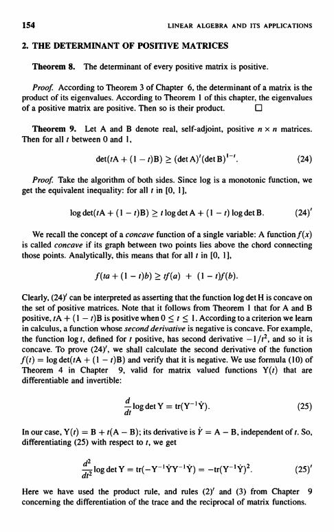
154 LINEAR ALGEBRA AND ITS APPLICATIONS
2. THE DETERMINANT OF POSITIVE MATRICES
Theorem 8. The determinant of every positive matrix is positive.
Proof. According to Theorem 3 of Chapter 6, the determinant of a matrix is theproduct of its eigenvalues. According to Theorem 1 of this chapter, the eigenvaluesof a positive matrix are positive. Then so is their product.
Theorem 9. Let A and B denote real, self-adjoint, positive n x n matrices.Then for all t between 0 and I,
det(tA + (1 - t) B) > (det A)'(det B)'-'. (24)
Proof. Take the algorithm of both sides. Since log is a monotonic function, weget the equivalent inequality: for all t in [0, 1],
log det(tA + (I - t)B) > t log det A + (1 - t) log det B. (24)'
We recall the concept of a concave function of a single variable: A function f(x)is called concave if its graph between two points lies above the chord connectingthose points. Analytically, this means that for all t in [0, 11,
f(ta + (I - t)b) > If(a) + (1 - t)f(b).
Clearly, (24)' can be interpreted as asserting that the function log det H is concave onthe set of positive matrices. Note that it follows from Theorem l that for A and Bpositive, to + (1 - t)B is positive when 0 < t < 1. According to a criterion we learnin calculus, a function whose second derivative is negative is concave. For example,the function log t, defined for t positive, has second derivative -1 /t2, and so it isconcave. To prove (24)', we shall calculate the second derivative of the functionf(t) = log det(tA + (I - t)B) and verify that it is negative. We use formula (10) ofTheorem 4 in Chapter 9, valid for matrix valued functions Y(t) that aredifferentiable and invertible:
dtlogdetY = tr(Y-1Y). (25)
In our case, Y(t) = B + t(A - B); its derivative is k = A - B, independent of t. So,differentiating (25) with respect to t, we get
z
dt2log detY = -tr(Y-I ')2. (25)'
Here we have used the product rule, and rules (2)' and (3) from Chapter 9concerning the differentiation of the trace and the reciprocal of matrix functions.

MATRIX INEQUALITIES 155
According to Theorem 3 of Chapter 6, the trace of a matrix is the sum of itseigenvalues; and according to Theorem 4 of Chapter 6, the eigenvalues of the squareof a matrix T are the square of the eigenvalues of T. Therefore
tr(Y-Y)2 = a (26)
where as are the eigenvalues of Y- "k. According to Theorem l 1' in Chapter 8, theeigenvalues aj of the product Y- I Y of a positive matrix Y-I and a self-adjoint matrixY are real. It follows that (26) is positive; setting this into (25)', we conclude that thesecond derivative of log det Y(t) is negative.
Second Proof. Define C as B- I A; by Theorem 11' of Chapter 8, the product C oftwo positive matrices has positive eigenvalues cj. Now rewrite the left-hand side of(24) as
det B(tB-1 A + (I -t)I) =detBdet(tC+(1 -t)I).
Divide both sides of (24) by det B; the resulting right-hand side can be rewritten as
(detA)'(detB)-' _ (detC)'.
What is to be shown is that
det(tC + (1 - t)I) > (det C)'.
Expressing the determinants as the product of eigenvalues gives
ll(tcj + I - t) fl ci, .
We claim that for all t between 0 and 1 each factor on the left is greater than thecorresponding factor on the right:
tc+(I -t)>c'.
This is true because c' is a convex function of t and equality holds when t = 0 ort= 1. O
Next we give a useful estimate for the determinant of a positive matrix.
Theorem 10. The determinant of a positive matrix H does not exceed theproduct of its diagonal elements:
det H < 11 hr;. (27)

156 LINEAR ALGEBRA AND ITS APPLICATIONS
Proof. Since H is positive, so are its diagonal entries. Define d; = 1/, anddenote by D the diagonal matrix with diagonal entries d,. Define the matrix B by
B = DHD.
Clearly, B is symmetric and positive and its diagonal entries are all I's. By themultiplicative property of determinants,
det B = det H det D2 =det H
fi h;,(28)
So (27) is the same as det B < 1. To show this, denote the eigenvalues of B bybi,... , b,,, positive quantities since B is a positive matrix. By the arithmetic-geometric mean inequality
fi b, < (> b;/n) .
We can rewrite this as
det B <(trB)
(29)n l
Since the diagonal entries of B are all l's, tr B = n, so det B < 1 follows.
Theorem 10 has this consequence.
Theorem 11. Let T be any n x n matrix whose columns are C, c2i ..., c,,. Thenthe determinant of T is in absolute value not greater than the product of the length ofits columns:
IdetTi < H ii ii.
Proof. Define H = T*T; its diagonal elements are
h« I;tj, lj,tl, _ I t i12 = II c, 1121 J
(30)
According to Theorem 1, T`T is positive, except when T is noninvertible, in whichcase det T = 0, so there is nothing to prove. We appeal now to Theorem tO anddeduce that
detH<fj 11c,112.
MATRIX INEQUALITIES 157
Since the determinant is multiplicative, and since detT* = detT,
detH = detT*detT = IdetTI2.
Combining the last two and taking its square root we obtain inequality (30) ofTheorem 11.
Inequality (30) is due to Hadamard and is useful in applications. In the real case ithas an obvious geometrical meaning: among all parallelepipeds with given sidelengths 11 cj 11, the one with the largest volume is rectangular.
We return to Theorem 9 about determinants; the first proof we gave for it used thedifferential calculus. We present now a proof based on integral calculus. This proofworks for real, symmetric matrices; it is based on an integral formula for thedeterminant of real positive matrices.
Theorem 12. Let H be an n x n real, symmetric, positive matrix. Then
n»/zJe-(x°ur)dx. (31)
det H R"
Proof It follows from inequality (5)' that the integral (31) converges. To evaluateit, we appeal to the spectral theorem for self-adjoint mappings, see Theorem 4' ofChapter 8, and introduce new coordinates
x = My, (32)
M an orthogonal matrix so chosen that the quadratic form is diagonalized:
(x, Hx) = (My, HM),) = (y, M*HMy) = E ajyj?. (33)
The aj are the eigenvalues of H. We substitute (33) into (31); since the matrix M is anisometry, it preserves volume as well: Idet MI = 1. In terms of the new variables theintegrand is a product of functions of single variables, so we can rewrite the rightside of (31) as a product of one-dimensional integrals:
f e-E",, dy = f 7J a-`jy dy = H j e-°,' dy; (34)
The change of variable /y = z turns each of the integrals on the right in (34) into
j4dze
aj
158
According to a result of calculus
so that the right-hand side of (34) equals
LINEAR ALGEBRA AND ITS APPLICATIONS
e12 7rn/2
f Uj (fl a,) 1/2
(35)
(34)
According to formula (15), Theorem 3 in Chapter 6 the determinant of H is theproduct of its eigenvalues; so formula (31) of Theorem 12 follows from (34) and(34)'.
EXERCISE 8. Look up a proof of the calculus result (35).
Proof of Theorem 9. We take in formula (35), H = to + (1 - t)B, where A, Bare arbitrary real, positive matrices:
det(tA+(1-:)B) R'
e-r(.r,Ax)e (I-r)(x,B.r)dx. (36)R^
We appeal now to Holder's inequality:
11u'I
/nJfdx < (JfPdx) (Jgcix)
where p, q are real, positive numbers such that
We take
f(x) = e-'(x,Ar) g(x) = e (1 rxx,B.r)1
and choose p = 1 It, q = 1/(I - t); we deduce that the integral on the right in (36) isnot greater than
r 1-r
C fe-(x.Ar)dxl/ (Je_dx)

MATRIX INEQUALITIES
Using formula (31) to express these integrals we get
r.n/2 l' nn/2 I -t 7rn/2
det A/ det B/ (det AY (det B) I '
159
Since this is an upper bound for (36), inequality (24) follows.
Formula (31) also can be used to give another proof of Theorem 10.
Proof. In the integral on the right in (31) we write the vector variable x asx = uei + z, where u is the first component of x and z the rest of them. Then
(x, Hx) = h, I u2 + 2ul (z) + (z, H I I z),
where 1(z) is some linear function of z. Setting this into (31) gives
,,n/2r Je__2hu1_H1dudz. (37)J
r r e-h,hn2+2n1-(z.Hjjz)du dz.
Adding and dividing by 2 gives
J
c+2
c_I
du dzf JeI11'
where c abbreviates e2nl. Since c is positive,
C+c- I
(37)'
>1.2
Therefore (37)' is bounded from below by
J
Je_Jhhu12e_Hh1dudz.
The integrand is now the product of a function of u and of z, and so is the product oftwo integrals, both of which can be evaluated by (31):
.I/2 (n-l)/2
det Hl l

160 LINEAR ALGEBRA AND ITS APPLICATIONS
Since this is a lower bound for the right-hand side of (37), we obtain thatdet H < h11 det H1 . Inequality (27) follows by induction on the size of H.
3. EIGENVALUES
In this section we present a number of interesting and useful results oneigenvalues.
Lemma 13. Let A be a self-adjoint map of a Euclidean space U into itself. Wedenote by p+ (A) the number of positive eigenvalues of A, and denote by p_ (A) thenumber of its negative eigenvalues.
p+(A) = maximum dimension of subspace S of U such that (Au, u) is positiveon S.
p_ (A) = maximum dimension of subspace S of U such (Au, u) is negative on S.
Proof. This follows from the minmax characterization of the eigenvalues of A;see Theorem 10, as well as Lemma 2 of Chapter 8.
Theorem 14. Let U and A be as in Lemma 13, and let V be a subspace of Uwhose dimension is one less than the dimension of U:
dim V = dim U - 1.
Denote by P orthogonal projection onto V. Then PAP is a self-adjoint map of U intoU that maps V into V; we denote by B the restriction of PAP to V. We claim that
p+ (A) - I < p+ (B) < p+ (A), (38)+
and
p- (A) - I <p-(B) <p-(A).(38)_
Proof. Let T denote a subspace of V of dimension p+ (B) on which B is positive:
(Bv,v)>0, vin T, v#0.
By definition of B, we can write this as
0 < (PAPv, v) = (APv, Pv).
MATRIX INEQUALITIES 161
Since v belongs to T, a subspace of V, Pv = v. So we conclude that A is positive on T;this proves that
p+ (B) < p+(A).
To estimate p+(B) from below, we choose a subspace S of U, of dimension p+(A)on which A is positive:
(Au, u) > 0, u in S, u 54 0.
Denote the intersection of S and V by T:
T=SnV.
We claim that the dimension of T is at most one less than the dimension of S:
dim S - 1 < dim T.
If S is a subspace of V, then T = S and dim T = dim S. If not, choose a basis inS: {s, , ... , Sk }. At least one of these. say si, does not belong to V; this means that s,has a nonzero component orthogonal to V. Then we can choose scalars a2.... , aksuch that
S2 - a2S1,...,Sk - akS,
belong to V. They are linearly independent, since s, , ... . sk are linearly independent.It follows that
dim S - 1 < dim T,
as asserted.We claim that B is positive on T. Take any v # 0 in T:
(Bv, v) = (PAPv, v) = (APv, Pv) = (Av, v),
since v belongs to V. Since v also belongs to S, (Av, v) > 0.Since p+(B) is defined as the dimension of the largest subspace on which B is
positive, and since dim T > dim S - 1, p+(B) > p+(A) - 1 follows. This completesthe proof of (38)+; (38)_ can be proved similarly.
An immediate consequence of Theorem 14 is the following theorem.
Theorem 15. Let U, V, A, and B be as in Theorem 14. Denote the eigenvaluesof A as a1,... , a,,, and denote those of B as b1,. .. , The eigenvalues of Bseparate the eigenvalues of A:
a, < b, < a2 < a,,. (39)
162 LINEAR ALGEBRA AND ITS APPLICATIONS
Proof. Apply Theorem 14 to A - c and B - c. We conclude that the number of b;less than c is not greater than the number of a; less than c, and at most one less. Weclaim that a; < b; j if not, we could choose b; < c < a; and obtain a contradiction.We can show analogously that b; < a;+,. This proves that a; < b; < a;+,, as assertedin (39).
Take U to be l° with the standard Euclidean structure, and take A to be any n x nself-adjoint matrix. Fix i to be some natural number between 1 and n, and take V toconsist of all vectors whose ith component is zero. Theorem 14 says that theeigenvalues of the ith principal minor of A separate the eigenvalues of A.
EXERCISE 9. Extend Theorem 14 to the case when dim V = dim U - m, wherem is greater than 1.
The following result is of fundamental interest in mathematical physics; see, forexample, Theorem 4 of Chapter 11.
Theorem 16. Let M and N denote self-adjoint k x k matrices satisfying
M < N. (40)
Denote the eigenvalues of M, arranged in increasing order, by m, < < Mk, andthose of N by n, < < nk. We claim that
mj < nj, j = 1,...,k. (41)
First Proof. We appeal to the minmax principle, Theorem 10 in Chapter 8,formula (40), according to which
,= min max (42)mjdims =j X ins (X, X)
(x, Nx)= i
,,,
(42)nj m n maxdimS=j x in S (X, x)
Denote by T the subspace of dimension j for which the minimum in (42) is reached,and denote by y the vector in T where (x, Mx)/(x,x) achieves its maximum; we takey to be normalized as 11 y 11 = 1. Then by (42),,,,
mj (Y, My),
while from (42),,,
(X Mx)
(Y, NY) < nj.

MATRIX INEQUALITIES 163
Since the meaning of (40) is that (y, My) < (y, Ny) for all y # 0, (41)follows.
If the hypothesis (40) is weakened to M < N, the weakened conclusion mj < njcan be reached by the same argument.
Second Proof. We connect M and N by a straight line:
A(t) = M + t(N - M); (43)
we also use calculus, as we have done so profitably in Section 1. Assuming for amoment that the eigenvalues of A(t) are distinct, we use Theorem 7 of Chapter 9 toconclude that the eigenvalues of A(t) depend differentiably on t, and we use formula(24) of that chapter for the value of the derivative. Since A is self-adjoint, we canidentify in this formula the eigenvector I of AT with the eigenvector h of A itself.Normalizing h so that II h II = 1, we have the following version of (24), Chapter 9,for the derivative of the eigenvalue a in Ah = ah:
ddt=(h'dAh)'
(43)'
For A(t) in (43), dA/dt = N - M is positive according to hypothesis (41); thereforethe right-hand side of (43)' is positive. This proves that da/dt is positive, andtherefore a(t) is an increasing function of t; in particular, a(0) < a(l). SinceA(0) = M, A(l) = N, this proves (41) in case A(t) has distinct eigenvalues for all tin [0, 1].
In case A(t) has multiple eigenvalues for a finite set of t, the above argumentshows that each ap(t) is increasing between two such values of t; that is enough todraw the conclusion (41). Or we can make use of the observation made at the end ofChapter 9 that the degenerate matrices form a variety of codimension 2 and can beavoided by changing M by a small amount and passing to the limit.
The following result is very useful.
Theorem 17. Let M and N be self-adjoint k x k matrices mj and nj theireigenvalues arrayed in increasing order. Then
Inl - mnI :5 11 M - NII. (44)
Proof Denote II M - N11 by d. It is easy to see that
N-dI<M<N+dI. (44)'
Inequality (44) follows from (44)' and (41).

164 LINEAR ALGEBRA AND ITS APPLICATIONS
EXERCISE 10. Prove inequality (44)'.
Wielandt and Hoffman have proved the following interesting result.
Theorem 18. Let M, N be self-adjoint k x k matrices and m1 and n1 theireigenvalues arranged in increasing order. Then
E(n1-m1)2<II N - MII
where II N - M 112 is the Hilbert-Schmidt norm defined by
IICII2IcijI2.
(45)
(46)
Proof The Hilbert-Schmidt norm of any matrix can be expressed as a trace:
II C II2 = trC`C. (46)'
For C self-adjoint,
IICII2=trC2. (46)"
Using (46)" we can rewrite inequality (45) as
1:(n1 - in)2 < tr(N - M)2.
Expanding both sides and using the linearity and commutativity of trace gives
n;' - 2n1m1 + mj < trN2 - 2 tr(NM) + tr M2. (47)
According to Theorem 3 of Chapter 6, the trace of N2 is the sum of the eigenvaluesof N2. According to the spectral mapping theorem, the eigenvalues of N2 are n1 .
Therefore
2Et trN, E m12 = trM-;
so inequality (47) can be restated as
njm1 > tr(NM). (47)'
To prove this we fix M and consider all self-adjoint matrices N whose eigenvaluesare ni, ... , nk. The set of such matrices N forms a bounded set in the space of all

MATRIX INEQUALITIES 165
self-adjoint matrices. By compactness, there is among these that matrix N thatrenders the right-hand side of (47)' largest. According to calculus, the maximizingmatrix Nmax has the following property: if N(t) is a differentiable function whosevalues are self-adjoint matrices with eigenvalues n i , ... , n,t, and N(O) = Nmax, then
dtr(N(t)M) = 0. (48)
LO
Let A denote any anti-self-adjoint matrix; according to Theorem 5, part (e),Chapter 9, eA` is unitary for any real values of t. Now define
N(t) = eA'Nmaxe-Ar (49)
Clearly, N(t) is self-adjoint and has the same eigenvalues as Nn,ax. According to part(d) of Theorem 5, Chapter 9,
teAt = AeA` = eA`A.
Using the rules of differentiation developed in Chapter 9, we get, upondifferentiating (49), that
dt N(t) = eA(ANmax - NmaxA)e-Ar
Setting this into (48) gives at t = 0
d tr(N(t)M) = trl dNM 1
r=0 \\\
= tr(ANmaxM - NmaxAM) = 0.r=0
Using the commutativity of trace, we can rewrite this as
tr(A(NmaxM - MNmax)) = 0. (48)'
The commutator of two self-adjoint matrices N.ax and M is anti-self-adjoint, so wemay choose
A = NmaxM - MNmax (50)
Setting this into (48)' reveals that trA2 = 0; since by (46)', for anti-self-adjoint A,
trA2 = -1: Inril2,
we deduce that A = 0, so according to (50) the matrices N,nax and M commute.Such matrices can be diagonalized simultaneously; the diagonal entries are nj and

166 LINEAR ALGEBRA AND ITS APPLICATIONS
in, in some order. The trace of NmaxM can therefore be computed in thisrepresentation as
E np tnj, (51)
where pp, j = 1, ... , k is some permutation of I,... , k. It is not hard to show, and isleft as an exercise to the reader, that the sum (51) is largest when the nj are arrangedin the same order as the mj, that is, increasingly. This proves inequality (47)' for Nmaxand hence for all N.
EXERCISE I I. Show that (51) is largest when n, and mj are arranged in the sameorder.
The next result is useful in many problems of physics.
Theorem 19. Denote by en,in(H) the smallest eigenvalue of a self-adjointmapping H in a Euclidean space. We claim that emirs is a concave function of H, thatis, that for0<t< 1,
emin(tL + (1 - t)M) > temin(L) + (1 - t)emin(M) (52)
for any pair of self-adjoint maps L and M. Similarly, emax(H) is a convex function ofH;forO<r<1,
emax(tL+ (I - t)M) < te,nax(L) + (1 - t)e,,,ax(M). (52)'
Proof. We have shown in Chapter 8, equation (37), that the smallest eigenvalueof a mapping can be characterized as a minimum:
emin (H) = min (x, Hx). (53)II.YII=i
Let y be a unit vector where (x, Hx), with H = tL + (1 - t)M reaches its minimum.Then
emin(tL + (1 - t)M) = t(y, Ly) + (I - t) (y, My)
> t min (x, Lx) + (1 - t) min (x, Mx)IIXII=I IIxII=I
= temin(L) + (1 - t)emin(M).
This proves (52). Since -emax(A) = emin(-A), the convexity of eax(A)follows.
Note that the main thrust of the argument above is that any function characterizedas the minimum of a collection of linear functions is concave.

MATRIX INEQUALITIES
4. REPRESENTATION OF ARBITRARY MAPPINGS
167
Every linear mapping Z of a complex Euclidean space into itself can bedecomposed, uniquely, as a sum of a self-adjoint mapping and an anti-self-adjointone:
Z = H + A, (54)
where
H* = H, A* = -A. (54)'
Clearly, if (54) and (54)' hold, Z' = H" + A* = H - A, so H and A are given by
H - Z+Z" -Z' - Z2
A2
H is called the self-adjoint part of Z, A the anti-self-adjoint part.
Theorem 20. Suppose the self-adjoint part Z is positive:
Z+Z' >0.
Then the eigenvalues of Z have positive real part.
Proof. Using the conjugate symmetry of scalar product in a complex Euclideanspace, and the definition of adjoint, we have the following identity for any vector h:
2 Re(Zh, h) = (Zh, h) + (Zh, h) = (Zh, h) + (h, Zh) = (Zh, h) + (Z*h, h)
= ((Z + Z')h,h).
Since we assumed in Theorem 18 that Z + Z" is positive, we conclude that for anyvector h # 0, (Zh, h) has positive real part.
Let h be an eigenvector for Z of norm 11 h 11= 1, with z the correspondingeigenvalue, Zh = zh. Then (Zh, h) = z has positive real part.
In Appendix 14 we give a far-reaching extension of Theorem 20.Theorem 20 can be used to give another proof of Theorem 4 about symmetrized
products: Let A and B be self-adjoint maps, and assume that A and AB + BA = Sare positive. We claim that then B is positive.
Second Proof of Theorem 4. Since A is positive, it has according to Theorem 1 asquare root AI/2 that is invertible. We multiply the relation
AB+BA=S
168 LINEAR ALGEBRA AND ITS APPLICATIONS
by A-112 from the right and the left:
A'12BA-1/z + A-1/2BAi/2 = A-1/2SA-"2. (55)
We introduce the abbreviation
Al/22BA-1/22 = Z (56)
and rewrite (55) as
Z + Z' = A-'12SA-'12. (55)'
Since S is positive, so, according to Theorem 1, is A-1/2SA-1/2; it follows from (55)'that Z + Z` is positive. By Theorem 20 the eigenvalues of Z have positive real part.
Formula (56) shows that Z and B are similar; therefore they have the sameeigenvalues. Since B is self-adjoint, it has real eigenvalues; so we conclude that theeigenvalues of B are positive. This, according to Theorem 1, guarantees that B ispositive.
EXERCISE 12. Prove that if the self-adjoint part of Z is positive, then Z isinvertible, and the self-adjoint part of Z` is positive.
The decomposition of an arbitrary Z as a sum of its self-adjoint and anti-self-adjointparts is analogous to writing a complex number as the sum of its real and imaginaryparts, and the norm is analogous to the absolute value. The next result strengthens thisanalogy. Let a denote any complex number with positive real part; then
- azz =wa+az
maps the right half-plane Re z > 0 onto the unit disc Iwi < 1. Analogously, we claimthe following:
Theorem 21. Let a be a complex number with Re a > 0. Let Z be a mappingwhose self-adjoint part Z + Z* is positive. Then
W = (I - aZ) (I + iiZ) -' (57)
is a mapping of norm less than 1. Conversely, 11 W 11 < I implies that Z + Z' > 0.
Proof. According to Theorem 20 the eigenvalues z of Z have positive real part. Itfollows that the eigenvalues of I + aZ, I + aZ are # 0; therefore I + aZ is invertible.For any vector x, denote (I + aZ)-1x = y; then by (57),
(I - aZ)y = Wx,

MATRIX INEQUALITIES
and by definition of y,
(I + aZ)y = X.
169
The condition II W II < 1 means that II Wx 112 < II x 112 for all x 54 0; in terms of ythis can be expressed as
11y -aZy112<II),+aZyll? (58)
Expanding both sides gives
IIy112+lal211Zy112-a(Zy,y)-a(y,Zy)<IIy112+1a1211Zy112+ a(Zy, y) + a(y, Zy). (59)
Cancelling identical terms and rearranging gives
0 < (a + a) [(Zy, y) + (y, Zy)] = 2 Re a[Z + Z*]y, y). (60)
Since we have assumed that Re a is positive and that Z + Z* > 0, (60) is true.Conversely, if (60) holds for all y, Z + Z* is positive.
Complex numbers z have not only additive but multiplicative decompositions:Z = reie, r > 0, Ie'BI = 1. Mappings of Euclidean spaces have similar decomposi-tions.
Theorem 22. Let A be a linear mapping of a complex Euclidean space intoitself. Then A can be factored as
A = RU, (61)
where R is a nonnegative self-adjoint mapping, and U is unitary. When A isinvertible, R is positive.
Proof Take first the case that A is invertible; then so is A*. For any x # 0,
(AA*x, x) = (A*x, A*x) = II As 112 > 0.
This proves that AA* is a positive mapping. According to Theorem 1, AA* has aunique positive square root R:
AA* = R2. (62)
Define U as R-IA; then U* = A*R-I, and so by (62),
UU* = R-IAA*R-' = R-'R 2R-I = I.

170 LINEAR ALGEBRA AND ITS APPLICATIONS
It follows that U is unitary. By definition of U as R-' A,
A = RU,
as asserted in (61).When A is not invertible, AA* is a nonnegative self-adjoint map; it has a uniquely
determined nonnegative square root R. Therefore
II Rx II2 = (Rx,Rx) = (R2x,x) = (AA*x,x)
= (A*x, A*x) = II A*x IIz (63)
Suppose Rx = Ry; then II R(x - y) II = 0, and so according to (63),II A*(x - y) II = 0, therefore Ax = A*y. This shows that for any u in the range ofR, it = Rx, we can define Vu as A*x. According to (63), V is an isometry; therefore itcan be extended to the whole space as a unitary mapping.
By definition, A* = VR; taking its adjoint gives A = RV*, which is relation (61)with V* = U. O
According to the spectral representation theorem, the self-adjoint map R can beexpressed as R = WDW*, where D is diagonal and W is unitary. Setting this into(61) gives A = WDW*U. Denoting W*U as V, we get
A = WDV, (64)
where W and V are unitary and D is diagonal, with nonnegative entries. Equation(64) is called the singular value decomposition of the mapping A. The diagonalentries of D are called the singular values of A; they are the nonnegative square rootsof the eigenvalues of AA*.
Take the adjoint of both sides of (61); we get
A" = U*R. (61)*
Denote A* as B, denote U* as V, and restate (61)* as
Theorem 22". Every linear mapping B of a complex Euclidean space can befactored as
B = MS,
where S is self-adjoint and nonnegative, and M is unitary.
Note. When B maps a real Euclidean space into itself, so do S and M.
EXERCISE 13. Let A be any mapping of a Euclidean space into itself. Show thatAA* and A*A have the same eigenvalues with the same multiplicity.
MATRIX INEQUALITIES 171
EXERCISE 14. Let A be a mapping of a Euclidean space into another Euclideanspace. Show that AA* and A*A have the same nonzero eigenvalues with the samemultiplicity.
EXERCISE 15. Give an example of a 2 x 2 matrix Z whose eigenvalues havepositive real part but Z + Z" is not positive.
EXERCISE 16. Verify that the commutator (50) of two self-adjoint matrices isanti-self-adjoint.
CHAPTER 1 1
Kinematics and Dynamics
In this chapter we shall illustrate how extremely useful the theory of linear algebra ingeneral and matrices in particular are for describing motion in space. There are threesections, on the kinematics of rigid body motions, on the kinematics of fluid flow,and on the dynamics of small vibrations.
1. THE MOTION OF RIGID BODIES
An isometry was defined in Chapter 7 as a mapping of a Euclidean space into itselfthat preserves distances. When the isometry relates the positions of a mechanicalsystem in three-dimensional real space at two different times, it is called a rigid bodymotion. In this section we shall study such motions.
Theorem 10 of Chapter 7 shows that an isometry M that preserves the origin islinear and satisfies
M*M=1. (1)
As noted in equation (33) of that chapter, the determinant of such an isometry is plusor minus 1; its value for all rigid body motions is 1.
Theorem 1 (Euler). An isometry M of three-dimensional real Euclidean spacewith determinant plus I that is nontrivial, that is not equal to I, is a rotation; it has auniquely defined axis of rotation and angle of rotation 0.
Proof. Points f on the axis of rotation remain fixed, so they satisfy
Mf =f: (2)
Linear Algebra and Its Applications. Second Edition, by Peter D. LaxCopyright(.) 2007 John Wiley & Sons, Inc.
172
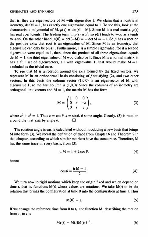
KINEMATICS AND DYNAMICS 173
that is, they are eigenvectors of M with eigenvalue 1. We claim that a nontrivialisometry, det M = 1, has exactly one eigenvalue equal to 1. To see this, look at thecharacteristic polynomial of M, p(s) = det(sI - M). Since M is a real matrix, p(s)has real coefficients. The leading term in p(s) is s3, so p(s) tends to +oc as s tendsto +oo. On the other hand, p(O) = det(-M) = - det M = -1. So p has a root onthe positive axis; that root is an eigenvalue of M. Since M is an isometry, thateigenvalue can only be plus 1. Furthermore, 1 is a simple eigenvalue; for if a secondeigenvalue were equal to 1, then, since the product of all three eigenvalues equalsdet M = 1, the third eigenvalue of M would also be 1. Since M is a normal matrix, ithas a full set of eigenvectors, all with eigenvalue 1; that would make M = I,excluded as the trivial case.
To see that M is a rotation around the axis formed by the fixed vectors, werepresent M in an orthonormal basis consisting off satisfying (2), and two othervectors. In this basis the column vector (1,0,0) is an eigenvector of M witheigenvalue 1; so the first column is (1,0,0). Since the columns of an isometry areorthogonal unit vectors and M = 1, the matrix M has the form
1 0 0M= 10 c -s
0 s c(3)
where c2 + s2 = 1. Thus c = cos 9, s = sin 9, 9 some angle. Clearly, (3) is rotationaround the first axis by angle 0. 11
The rotation angle is easily calculated without introducing a new basis that bringsM into form (3). We recall the definition of trace from Chapter 6 and Theorem 2 inthat chapter, according to which similar matrices have the same trace. Therefore, Mhas the same trace in every basis; from (3),
trM = I + 2 cos 9, (4)
hence
2(4)'
We turn now to rigid motions which keep the origin fixed and which depend ontime t, that is, functions M(t) whose values are rotations. We take M(t) to be therotation that brings the configuration at time 0 into the configuration at time t. Thus
M(0) = I. (5)
If we change the reference time from 0 to ti, the function M, describing the motionfrom t, to t is
tr M - lcos 9 =
MI(t) = M(t)M(t,)-'. (6)
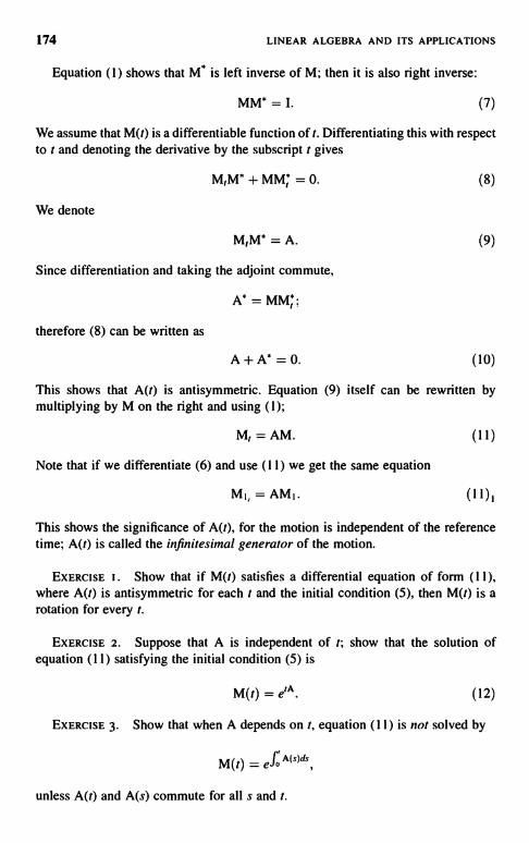
174 LINEAR ALGEBRA AND ITS APPLICATIONS
Equation (1) shows that Mµ is left inverse of M; then it is also right inverse:
(7)
We assume that M(t) is a differentiable function of t. Differentiating this with respectto t and denoting the derivative by the subscript t gives
M,M" + MM* = 0. (8)
We denote
M,M* = A. (9)
Since differentiation and taking the adjoint commute,
A" = MM;;
therefore (8) can be written as
A+A*=0. 10)
This shows that A(t) is antisymmetric. Equation (9) itself can be rewritten bymultiplying by M on the right and using (1);
Mt = AM.
Note that if we differentiate (6) and use (11) we get the same equation
M,, = AM,. (11),
This shows the significance of A(t), for the motion is independent of the referencetime; A(t) is called the infinitesimal generator of the motion.
EXERCISE 1. Show that if M(t) satisfies a differential equation of form (11),where A(t) is antisymmetric for each t and the initial condition (5), then M(t) is arotation for every t.
EXERCISE 2. Suppose that A is independent of t; show that the solution ofequation (11) satisfying the initial condition (5) is
M(t) = edA (12)
EXERCISE 3. Show that when A depends on t, equation (11) is not solved by
M(t) = ef0 A(s)ds
unless A(t) and A(s) commute for all s and t.

KINEMATICS AND DYNAMICS 175
We investigate now M(t) near t = 0; we assume that M(t) 34 I for t # 0; then foreach t # 0, M(t) has a unique axis of rotation f(t):
M(t) f (t) = f (t).
We assume that f(t) depends differentiably on t; differentiating the precedingformula gives
Mf+Mf,=f,.
We assume that both f (t) and f,(t) have limits as t -> 0. Letting t -ti 0 in this formulagives
Mcf(0) + M(0)f, =f'. (13)
Using (11) and (5), we get
A(0) f (0) = 0. (14)
We claim that if A(O) 0 0 then this equation has essentially one solution, that is, allare multiples of each other. To see that there is a nontrivial solution, recall that Ais antisymmetric; for n odd,
det A = det A* = det(-A) = (-1)" det A = - det A,
from which it follows that det A = 0, that is, the determinant of an antisymmetricmatrix of odd order is zero. This proves that A is not invertible, so that (14) has anontrivial solution. This fact can also be seen directly for 3 x 3 matrices by writingout
0 a bA= -a 0 c (15)
-b -c 0
Inspection shows that
f=-c
b , (16)
-a
lies in the nullspace of A.
EXERCISE 4. Show that if A in (15) is not equal to 0, then all vectors annihilatedby A are multiples of (16).
EXERCISE 5. Show that the two other eigenvalues of A are ±i a2 + b2 + c2.

176 LINEAR ALGEBRA AND ITS APPLICATIONS
EXERCISE 6. Show that the motion M(t) described by (12) is rotation around theaxis through the vector f given by formula (16). Show that the angle of rotation ist a2 -b2+ c2. (Hint: Use formula (4)'.)
The one-dimensional subspace spanned by f(0) satisfying (14), being the limit ofthe axes of rotation f(t), is called the instantaneous axis of rotation of the motion att = 0.
Let 0(t) denote the angle through which M(t) rotates. Formula (4)' shows that 0(t)is a differentiable function of t; since M(0) = I, it follows that trM(0) = 3, and soby (4)' cos 0(0) = 1. This shows that 0(0) = 0.
We determine now the derivative of 0 at t = 0. For this purpose we differentiate(4)' twice with respect to t. Since trace is a linear function of matrices, the derivativeof the trace is the trace of the derivative, and so we get
0-02 1
cos0=2trM,,.
Setting t = 0 gives
0;(0) = - I (17)
To express M,,(0) we differentiate (11):
M,, = A,M + AM, = A,M + A2M.
Setting t = 0 gives
M,,(0) = A,(0) + A2(0).
Take the trace of both sides. Since A(t) is antisymmetric for every t, so is A,; the traceof an antisymmetric matrix being zero, we get trA2(0). Using formula(15), a brief calculation gives
trA2(0) = -2(a2 + b2 + c2).
Combining the last two relations and setting it into (17) gives
0,(0) = a 2 + b 2 + c2.
Compare this with (16); we get
10,1 = V1. (18)
The quantity 0, is called the instantaneous angular velocity of the motion; the vectorf given by (16) is called the instantaneous angular velocity vector.

KINEMATICS AND DYNAMICS
EXERCISE 7. Show that the commutator
[A, B] = AB - BA
of two antisymmetric matrices is antisymmetric.
177
EXERCISE 8. Let A denote the 3 x 3 matrix (15); we denote the associated nullvector (16) byfA. Obviously, f depends linearly on A.
(a) Let A and B denote two 3 x 3 antisymmetric matrices. Show that
trAB = -2(fA,fa),
where (,) denotes the standard scalar product for vectors in Q.
EXERCISE 9. Show that the cross product can be expressed as
fA,BI =fA xfB
2. THE KINEMATICS OF FLUID FLOW
The concept of angular velocity vector is also useful for discussing motions that arenot rigid, such as the motion of fluids. We describe the motion of a fluid by
x = x(y, t); (19)
here x denotes the position of a point in the fluid at time i that at time zero waslocated at y:
x(y,0) = y. (19)0
The partial derivative of x with respect to t, y fixed, is the velocity v of the flow:
atx(y,t) = x,(y,r) = v(y,t).
The mapping y -> x, t fixed, is described locally by the Jacobian matrix
J(y, t) = -y , that is, Jy = y .
It follows from (19)0 that
(20)
(21)
J(y, 0) = I. (21)0
178 LINEAR ALGEBRA AND ITS APPLICATIONS
We learn in the integral calculus of functions of several variables that thedeterminant of the Jacobian J(y, t) is the factor by which the volume of the fluidinitially at y is expanded at time t. We assume that the fluid is never compressed tozero. Since at t = 0, det J(y, 0) = det I = 1 is positive, it follows that det J(y, t) ispositive for all t.
We appeal now to Theorem 22' of Chapter 10 to factor the matrix J as
J = MS, (22)
M = M(y, t) a rotation, S = S(y, t) selfadjoint and positive. Since J is real, so are Mand S. Since det J and det S are positive, so is det M. Since J(t) I as t -> 0, itfollows, see the proof of Theorem 22 in Chapter 10, that also S and M --> I as t -> 0.
It follows from the spectral theory of self-adjoint matrices that S acts ascompression or dilation along the three axes that are the eigenvectors of S. M isrotation; we shall calculate now the rate of rotation by the action of M. To do this wedifferentiate (22) with respect to t:
J, = MS, + M,S. (22)'
We multiply (22) by M* on the left; since M*M = I we get
M*J = S.
We multiply this relation by M, from the left, make use of the differential equationM, = AM, see (11), and that MM* = I.
Setting this into (22)' gives
Set t = 0:
M,S = AMM"J = AJ.
J,=MS,+AJ.
J,(O) = S,(O) + A(O).
(23)
(23)0
We recall from (10) that A(O) is anti-self-adjoint. S, on the other hand, being thederivative of self-adjoint matrices, is itself self-adjoint. Thus (23)0 is thedecomposition of J,(O) into its self-adjoint and anti-self-adjoint parts.
Differentiating (21) with respect to t and using (20) gives
J, =09V
, (24)
09)
that is,
J,j _av`
(24)'ayi
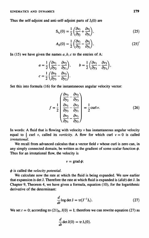
KINEMATICS AND DYNAMICS
Thus the self-adjoint and anti-self-adjoint parts of J,(0) are
s..(o)
=I /av;
+av l ,
2 ayeTY,I /av; _ avjl
(0)2 ayi ayr
In (15) we have given the names a, b, c to the entries of A:
1 (OVI _ 8v2) b _ I (avi _ av3'\
a-2 aye ayi 2 5y3 a)'i '
I 09V2 av3
= 2 ay3 - aye
Set this into formula (16) for the instantaneous angular velocity vector:
f_I
2
av3 av2
aye Y3
av, av3
ay3 OYi
av2 avi
OYI - aye
= 2 curl v.
179
(25)
(25)'
(26)
In words: A fluid that is flowing with velocity v has instantaneous angular velocityequal to 2 curl v, called its vorticity. A flow for which curl v = 0 is calledirrotational.
We recall from advanced calculus that a vector field v whose curl is zero can, inany simply connected domain, be written as the gradient of some scalar functionThus for an irrotational flow, the velocity is
v = grad 0;
is called the velocity potential.We calculate now the rate at which the fluid is being expanded. We saw earlier
that expansion is det J. Therefore the rate at which fluid is expanded is (dldt) det J. InChapter 9, Theorem 4, we have given a formula, equation (10), for the logarithmicderivative of the determinant:
dtlogdetJ = tr(JJ,). (27)
We set t = 0; according to (21)0, J(0) = I; therefore we can rewrite equation (27) as
dtdetJ(0) = trJ,(0).

180 LINEAR ALGEBRA AND ITS APPLICATIONS
By (24)', J,ij = Ovi/Oyi; therefore
(27)'dt 8yi
In words: A fluid that is flowing with velocity v is being expanded at the rate div v.That is why the velocity field of an incompressible fluid is divergence free.
3. THE FREQUENCY OF SMALL VIBRATIONS
By small vibrations we mean motions of small amplitude about a point ofequilibrium. Since the amplitude is small, the equation of motion can be taken to belinear. Let us start with the one-dimensional case, the vibration of a mass m under theaction of a spring. Denote by x = x(t) displacement of the mass from equilibriumx = 0. The force of the spring, restoring the mass toward equilibrium, is taken tobe -kx, k a positive constant. Newton's law of motion, force equals mass timesacceleration, says that,
mx + kx = 0; (28)
here the dot symbol denotes differentiation with respect to t.Multiply (28) by x:
mxX + kxk =dt
I2,nX2 + 2x21 = 0;
therefore
Zmx2+2x2=E(29)
is a constant, independent of t. The first term in (29) is the kinetic energy of a mass inmoving with velocity x; the second term is the potential energy stored in a springdisplaced by the amount x. That their sum, E, is constant expresses the conservationof total energy.
The equation of motion (28) can be solved explicitly: All solutions are of the form
x(t) = a sin t + 9) (30)
a is called the amplitude, 0 the phase. All solutions (30) are periodic in t, with periodp = 27r m/k. The frequency, defined as the reciprocal of the period, is the numberof vibrations the system performs per unit time:
frequency =IV
(31)2n m

KINEMATICS AND DYNAMICS 181
We note that part of this result can be deduced by dimensional analysis. From thefact that kx is a force, we deduce that
dim k length = dim forcemass length
= mass acceleration =time'
So
dimk --mass
time2
The only quantity constructed out of the two parameters in. and k whose dimension istime is const VG-ilk. So we conclude that the period p of motion is given by
p = cons[ m/k.
Formula (31) shows that frequency is an increasing function of k, and a decreasingfunction of in. Intuitively this is clear; increasing k makes the spring stiffer and thevibration faster; the smaller the mass, the faster the vibration.
We present now a far-reaching generalization of this result to the motion of asystem of n masses on a line, each linked elastically to each other and to the origin.Denote by xi the position of the ith particle; Newton's second law of motion for theith particle is
mixi -f, = 0, (32)
where f, is the total force acting on the ith particle and ini is its mass. We take theorigin to be a point of equilibrium for the system, that is, all f, are zero when all the xiare zero.
We denote by f,1 the force exerted by the jth particle on the ith. According toNewton's third law, the force exerted by the ith particle on the jth is -fl. We take f1to be proportional to the distance of xi and x1:
f,=ki1(xx-xi), i0j (33)
To satisfy f1 = fi we take kit = kki. Finally, we take the force exerted from theorigin on particle i to be -kixi. Altogether we have
f = k ; 1 x 1 , kii = -ki - k, . (33)'i i
We now rewrite the system (32) in matrix form as
Mx+Kx=0; (32)'

182 LINEAR ALGEBRA AND ITS APPLICATIONS
here x denotes the vector (XI, X2, ... , XIX, M is a diagonal matrix with entries m,, andthe elements of K are -k, from (33)'. The matrix K is real and symmetric; thentaking the scalar product of (32)' with x we obtain
(x, Mx) + (x, Kx) = 0.
Using the symmetry of K and M we can rewrite this as
from which we conclude that
ddt [2 (x,
M.,)+ I (x, Kx)J = 0,
20c,Mx)+I(x,Kx)=E (34)
is a constant independent of t. The first term on the left-hand side is the kineticenergy of the masses, the second term the potential energy stored in the system whenthe particles have been displaced from the origin to x. That their sum, E, is constantduring the motion is an expression of the conservation of total energy.
We assume now that all the forces are attractive, that is, that ki, and ki are positive.We claim that then the matrix K is positive. For proof see Theorem 5 at the end ofthis chapter. According to inequality (5)' of Chapter 10, a positive matrix K satisfiesfor all x,
a1Ix112<(x,Kx), a positive.
Since the diagonal matrix M is positive, combining the above inequality with (34)gives
a11x112<E.
This shows that the amplitude 11 x 11 is uniformly bounded for all time, andfurthermore if the total energy E is sufficiently small, the amplitude 11 x 11 is small.
A second important consequence of the positivity of K is
Theorem 2. Solutions of the differential equation (32)' are uniquelydetermined by their initial data x(0) and x(0). That is, two solutions that have thesame initial data are equal for all time.
Proof. Since equation (32)' is linear, the difference of two solutions is again asolution. Therefore it is sufficient to prove that if a solution x has zero initial data,then x(t) is zero for all t. To see this, we observe that if x(0) = 0, x(0) = 0, thenenergy E at t = 0 is zero. Therefore energy is zero for all t. But energy defined by(34) is the sum of two nonnegative terms; therefore each is zero for all t.
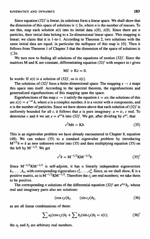
KINEMATICS AND DYNAMICS 183
Since equation (32)' is linear, its solutions form a linear space. We shall show thatthe dimension of this space of solutions is <2n, where n is the number of masses. Tosee this, map each solution x(t) into its initial data x(0), z(0). Since there are nparticles, their initial data belong to a 2n-dimensional linear space. This mapping islinear; we claim that it is 1-to-1. According to Theorem 2, two solutions with thesame initial data are equal; in particular the nullspace of this map is {0}. Then itfollows from Theorem 1 of Chapter 3 that the dimension of the space of solutions is< 2n.
We turn now to finding all solutions of the equations of motion (32)'. Since thematrices M and K are constant, differentiating equation (32)' with respect to t gives
M.F+Ki=0.
In words: If x(t) is a solution of (32)', so is x(t).The solutions of (32)' form a finite-dimensional space. The mapping x -p x maps
this space into itself. According to the spectral theorem, the eigenfunctions andgenerealized eigenfunctions of this mapping span the space.
Eigenfunctions of the map x i satisfy the equation x = ax; the solutions of thisare x(t) = e-"' h, where a is a complex number, h is a vector with n components, andn is the number of particles. Since we have shown above that each solution of (32)' isuniformly bounded for all t, it follows that a is pure imaginary: a = ic, c real. Todetermine c and h we set x = e'h into (32)'. We get, after dividing by e"', that
c2Mh = Kh. (35)
This is an eigenvalue problem we have already encountered in Chapter 8, equation(48). We can reduce (35) to a standard eigenvalue problem by introducingM112h = k as new unknown vector into (35) and then multiplying equation (35) onthe left by M-1/2. We get
c2k = M-1/2KM-'12k. (35)'
Since M-'12KM-'12 is self-adjoint, it has n linearly independent eigenvectorski, ... , k,,, with corresponding eigenvalues ci , .... c,2,. Since, as we shall show, K is apositive matrix, so is M-'12KM-'"2. Therefore the cJ are real numbers; we take themto be positive.
The corresponding n solutions of the differential equation (32)' are e"'"'h1, whosereal and imaginary parts also are solutions:
(cos cjt)hj, (sin c1t)hj, (36)
as are all linear combinations of them:
aj(cos clt)hj + bb(sin cct)hj = x(t); (36)'
the ai and bl are arbitrary real numbers.
184 LINEAR ALGEBRA AND ITS APPLICATIONS
Theorem 3. Every solution of the differential equation (32)' is of form (36).
Proof. Solutions of the form (36)' form a 2n-dimensional space. We have shownthat the set of all solutions is a linear space of dimension <2n. It follows that allsolutions are of form (36)'.
ExERCISE 10. Verify that solutions of the form (36) form a 2n-dimensionallinear space.
The special solutions (36); are called normal modes; each is periodic, with period2ir/cj and frequency cJ/2n. These are called the natural frequencies of themechanical system governed by equation (32)'.
Theorem 4. Consider two differential equations of form (32)':
Mz+Kx=0, Ny+Ly=O,
M, K, N, L positive, real n x n matrices. Suppose that
M > N and K < L.
(37)
(38)
Denote 2ir times the natural frequencies of the first system, arranged in increasingorder by c, < ... < c,,, and those of the second system by d, < ... < d,,. We claimthat
cj<dj, j=1,...,n. (39)
Proof. We introduce an intermediate differential equation
Mi + Lz = 0,
Denote its natural frequencies by f /2ir. In analogy with equation (35), the f satisfy
f2Mh = Lh,
where h is an eigenvector. In analogy with equation (35)', we can identify thenumbersf2 as the eigenvalues of
M-'/2LM-1"2.
We recall that the numbers c2 are eigenvalues of
M-1/2KM'1/2.

KINEMATICS AND DYNAMICS 185
Since K is assumed to be < L, it follows from Theorem 1 of Chapter 10 that also
M-'12KM-1/2 < M-1/2LM- 1/2.
Then it follows from Theorem 16 of Chapter 10 that
c < f2, j= 1,...,n. (39)'
On the other hand, in analogy with equation (35)", we can identify the reciprocals1 /f2 as the eigenvalues of
L-1/2ML-1/2
whereas the reciprocals 1 /d2 are the eigenvalues of
L-1/2NL-1/2.
Since N is assumed, to be < M, it follows as before that
L-1/2NL-1/2 < L-'12ML-112,
so by Theorem 16 of Chapter 10
1 1
d f 2
We can combine inequalities (39)' and (39)" to deduce (39).
(39)"
Note: If either of the inequalities in (38) is strict, then all the inequalities in (39)are strict.
The intuitive meaning of Theorem 4 is that if in a mechanical system we stiffenthe forces binding the particles to each other and reduce the mass of all the particles,then all natural frequencies of the system increase.
We supply now the proof of the positivity of the matrix K.
Theorem 5. Suppose that the numbers k; and k, , i # j are positive. Then thesymmetric matrix K,
Ky=-k,,, i#j; K,,=k;+Eki (40)iii
is positive.

186 LINEAR ALGEBRA AND ITS APPLICATIONS
Proof. It suffices to show that every eigenvalue a of K is positive:
Ku = au. (41)
Normalize the eigenvector u of K so that the largest component, say u;, equals 1, andall others are < 1. The ith component of (41) is
Ki,+EK,,u1=a.i#i
Using the definition (40) of the entries of K, this can be rewritten as
k; +Ek1(1-u1)=a.1#i
The left-hand side is positive; therefore, so is the right-hand side a.
For a more general result, see Appendix 7.
CHAPTER 12
Convexity
Convexity is a primitive notion, based on nothing but the bare bones of the structureof linear spaces over the reals. Yet some of its basic results are surprisingly deep;furthermore, these results make their appearance in an astonishingly wide variety oftopics.
X is a linear space over the reals. For any pair of vectors x, yin X, the line segmentwith endpoints x and y is defined as the set of points in X of form
ax+(1-a)y, 0<a<1. (1)
Definition. A set K in X is called convex if, whenever x and y belong to K, allpoints of the line segment with endpoints x, y also belong to K.
Examples of Convex Sets
(a) K = the whole space X.(b) K = 4, the empty set.(c) K = {x}, a single point.(d) K = any line segment.(e) Let l be a linear function in X; then the sets
l(x) = c, called a hyperplane, (2)
l(x) < c, called an open half-space, (3)
l(x) < c, called a closed half-space, (4)
are all convex sets.
Linear Algebm and Its Applications, Second Edition, by Peter D. LaxCopyright Q 2007 John Wiley & Sons, Inc.
187

188 LINEAR ALGEBRA AND ITS APPLICATIONS
Concrete Examples of Convex Sets
(f) X the space of all polynomials with real coefficients, K the subset of allpolynomials that are positive at every point of the interval (0, 1).
(g) X the space of real, self-adjoint matrices, K the subset of positive matrices.
EXERCISE I. Verify that these are convex sets.
Theorem 1. (a) The intersection of any collection of convex sets is convex.(b) The sum of two convex sets is convex, where the sum of two sets K and H is
defined as the set of all sums x + y, x in K, yin H.
EXERCISE 2. Prove these propositions.
Using Theorem 1, we can build an astonishing variety of convex sets out of a fewbasic ones. For instance, a triangle in the plane is the intersection of three half-planes.
Definition. A point x is called aninterior point of a set S in X if for everyy in X,x + yt belongs to S for all sufficiently small positive t.
Definition. A convex set K in X is called open if every point in it is an interior point.
EXERCISE 3. Show that an open half-space (3) is an open convex set.
EXERCISE 4. Show that if A is an open convex set and B is convex, then A + B isopen and convex.
Definition. Let K be an open convex set that contains the vector 0. We define itsgauge function pK = p as follows: For every x in X,
p(x) = inf r, r > O and x in K.r (5)
EXERCISE 5. Let X be a Euclidean space, and let K be the open ball of radius acentered at the origin: 11 x 11 < a.
(i) Show that K is a convex set.(li) Show that the gauge function of K is p(x) = 11 x 11/a.
EXERCISE 6. In the (u, v) plane take K to be the quarter-plane u < 1, v < 1.Show that the gauge function of K is
1 0 if U<0' V<0'v if 0<v, u<0,_
p(u, v)u if 0 < u, V<0'
max(u, v) if 0<u, 0<v.
CONVEXITY 189
Theorem 2. (a) The gauge function p of an open convex set K that contains theorigin is well-defined for every x.
(b) p is positive homogeneous:
p(ax) = ap(x) for a > 0. (6)
(c) p is subadditive:
P(x + y) < P(x) + P(y) (7)
(d) p(x) < 1 iff x is in K.
Proof. Call the set of r > 0 for which x/r is in K admissible for x. To prove(a) we have to show that for any x the set of admissible r is nonempty. This followsfrom the assumption that 0 is an interior point of K.
(b) follows from the observation that if r is admissible for x and a > 0, then ar isadmissible for ax.
(c) Let s and t be positive numbers such that
P(x) < s, P(y) < t. (8)
Then by definition of p as inf, it follows that s and t are admissible for x and y;therefore x/s and y/t belong to K. The point
x+), S X t y
s+t s+tss+tt (9)
lies on the line segment connecting x/s and y/t. By convexity, (x + y)/s + t belongsto K. This shows that s + t is admissible for x + y; so by definition of p,
p(x + y) < s + t. (10)
Since s and t can be chosen arbitrarily close to p(x) and p(y), (c) follows.(d) Suppose p(x) < 1; by definition there is an admissible r < 1. Since r is
admissible, x/r belongs to K. The identity x = rx/r + (1 - r)0 shows that x lies on theline segment with endpoints 0 and x/r, so by convexity belongs to K.
Conversely, suppose x belongs to K; since x is assumed to be an interior point of Kthe point x + ex belongs to K for E > 0 but small enough. This shows thatr = 1 /(1 + E) is admissible, and so by definition
P(x)<1
1+E
This completes the proof of the theorem.
190 LINEAR ALGEBRA AND ITS APPLICATIONS
EXERCISE 7. Let p be a positive homogeneous, subadditive function. Prove thatthe set K consisting of all x for which p(x) < I is convex and open.
Theorem 2 gives an analytical description of the open convex sets. There is another,dual description. To derive it we need the following basic, and geometrically intuitiveresults.
Theorem 3. Let K be an open convex set, and let y be a point not in K. Thenthere is an open half-space containing K but not y.
Proof. An open half-space is by definition a set of points satisfying inequality1(x) < c; see (3). So we have to construct a linear function 1 and a number c such that
l(x) < c for all x in K, (11)
l(y) = c (12)
We assume that 0 lies in K; otherwise shift K. Set x = 0 in (11); we get 0 < c. Wemay set c = 1. Let p be the gauge function of K; according to Theorem 2, points of Kare characterized by p(x) < 1;. It follows that (11) can be stated so:
If p(x) < 1, then I(x) < I. (11)'
This will certainly be the case if
1(x) < p(x) for all x. (13)
So Theorem 3 is a consequence of the following: there exists a linear function Iwhich satisfies (13) for all x and whose value at ), is 1. We show first that the tworequirements are compatible. Requiring 1(y) = 1 implies by linearity that 1(ky) = kfor all k. We show now that (13) is satisfied for all x of form ky; that is, for all k.
k = 1(ky) < p(ky),
For k positive, we can by (6) rewrite this as
k < kp(y),
(14)
(14)'
true because y does not belong to K and so by part (d) of Theorem 2, p(y) > 1. Onthe other hand, inequality (14) holds for k negative; since the left-hand side is lessthan 0, the right-hand side, by definition (5) of gauge function, is positive.
The remaining task is to extend I from the line through y to all of X so that (13) issatisfied. The next theorem asserts that this can be done.
CONVEXITY 191
Theorem 4 (Hahn-Banach). Let p be a real-valued positive homogeneoussubadditive function defined on a linear space X over R. Let U be a subspace of X onwhich a linear function is defined, satisfying (13):
1(u) < p(u) for all u in U. (13)U
Then l can be extended to all of X so that (13) is satisfied for all x.
Proof. Proof is by induction; we show that I can be extended to a subspace Vspanned by U and any vector z not in U. That is, V consists of all vectors of form
v = u + tz, u in U. t any real number.
Since 1 is linear
1(v) = 1(u) + tl(z);
this shows that the value of 1(z) = a determines the value of l on V
1(v) = 1(u) + ta.
The task is to choose a so that (13) is satisfied: 1(v) < p(v), that is,
1(u) + to < p(u + tz)
for all u in U and all real t.We divide (13),, by ItI. Fort > 0, using positive homogeneity of p and linearity of
l we get
l(u*) + a < p(u* + z), (14)+
where u* denotes ult. For t < 0 we obtain
1(u**) - a < p(u** - z), (14)_
where u** denotes -u/t. Clearly, (13),, holds for all u in U and all real tiff (14)+ and(14)_ hold for all u" and u*', respectively, in U.
We rewrite (14), as
I(u**) - p(u**- z) < a < p(u* + z) - l(u*);
the number a has to be so chosen that this holds for all u* and u** in U. Clearly, this ispossible iff every number on the left is less than or equal to any number on the right,that is, if
1(u**) - p(u** - z) < p(u" + z) -1(u*)
(15)
192 LINEAR ALGEBRA AND ITS APPLICATIONS
for all u*, u" in U. We can rewrite this inequality as
l(u**) + 1(u*) < p(u* + z) + p(u" - z).
By linearity, the left-hand side can be written as l(u** + u*); since (13)U holds,
1(u** + u*)<
p(u** + u*).
Since p is subadditive,
P(u** + u*) = P(u** - z + u* + z) < p(u** - z) + P(u* + z).
This proves (15)', which shows that l can be extended to V. Repeating this n times,we extend l to the whole space X. 0
This completes the proof of Theorem 3. 0
Note. The Hahn-Banach Theorem holds in infinite-dimensional spaces. Theproof is the same, with some added logical prestidigitation.
The following result is an easy extension of Theorem 3.
Theorem 5. Let K and H be open convex sets that are disjoint. Then there is ahyperplane that separates them. That is, there is a linear function 1 and a constant dsuch that
1(x) < d on K, 1(y) > d on H.
Proof. Define the difference K - H to consist of all differences x - y, x in K, y inH. It is easy to verify that this is an open, convex set. Since K and H are disjoint,K - H does not contain the origin. Then by Theorem 3, with y = 0, and thereforec = 0, there is a linear function 1 that is negative on K - H:
1(x - y) < 0 for x in K,y in H.
We can rewrite this as
1(x) < 1(y) for all x in K, y in H.
It follows from the completeness of real numbers that there is a number d such thatfor x in K, y in H,
1(x) < d < 1(y)
Since both K and H are open, the sign of equality cannot hold; this provesTheorem 5. 0
CONVEXITY 193
We show next how to use Theorem 3 to give a dual description of open convexsets.
Definition. Let S be any set in X. We define its support function qs on the dualX' of X as follows:
qs(l) = sup 1(x), (16)xinS
where 1 is any linear function.
Remark. qs(l) may be oo for some 1.
EXERCISE 8. Prove that the support function qs of any set is .subadditive; that is,it satisfies qs(m + 1) < qs(m) + qs(1) for all 1, in in X'.
EXERCISE 9. Let S and T be arbitrary sets in X. Prove that qs+T(1) _qs(1) + qT(1)
EXERCISE 10. Show that max{gs(1),gT(1)}.
Theorem 6. Let K be an open convex set, qK its support function. Then xbelongs to K iff
1(x) < qK(l) (17)
for all I in X'.
Proof It follows from definition (16) that for every x in K 1(x) < qK(l) forevery 1; therefore the strict inequality (17) holds for all interior points x in K. To seethe converse, suppose that y is not in K. Then by Theorem 3 there is an l such thatl(x) < I for all x in K, but 1(y) = 1 Thus
l(y) = I > sup 1(x) = qK(l); (18)xinK
this shows that y not in K fails to satisfy (17) for some 1. This provesTheorem 6.
Definition. A convex set K in X is called closed if every open segmentax + (1 - a)y, 0 < a < 1, that belongs to K has its endpoints x and y in K.
Examples
The whole space X is closed.The empty set is closed.

194 LINEAR ALGEBRA AND ITS APPLICATIONS
A set consisting of a single point is closed.An interval of form (1) is closed.
EXERCISE 11. Show that a closed half-space as defined by (4) is a closed con-vex set.
EXERCISE 12. Show that the closed unit ball in Euclidean space, consisting of allpoints 11 x 11 < 1, is a closed convex set.
EXERCISE 13. Show that the intersection of closed convex sets is a closedconvex set.
Theorems 2, 3, and 6 have their analogue for closed convex sets.
Theorem 7. Let K be a closed, convex set, and y a point not in K. Then there is aclosed half-space that contains K but not y.
Sketch of Proof. Suppose K contains the origin. If K has no interior points, it liesin a lower-dimensional subspace. If it has an interior point, we choose it to be theorigin. Then the gauge function PK of K can be defined as before. If x belongs to K,we may choose in the definition (5) of PK the value r = 1; this shows that for x in K,p(x) < I, Conversely, if pK(x) < 1, then by (5) x/r belongs to K for some r < 1.Since 0 belongs to K, by convexity so does x. If pK(x) = 1, then for all r > l,x/rbelongs to K. Since K is closed, so does the endpoint x. This shows that K consistsof all points x which satisfy pK(x) < 1. We then proceed as in the proof ofTheorem 3. O
Theorem 7 can be rephrased as follows.
Theorem 8. Let K be a closed, convex set, qK its support function. Then xbelongs to K if
l(x) <_ qK(l) (19)
for all l in V.
EXERCISE 14. Complete the proof of Theorems 7 and 8.
Both Theorems 6 and 8 describe convex sets as intersections of half-spaces, openand closed, respectively.
Definition. Let S be an arbitrary set in X. The closed convex hull of S is definedas the intersection of all closed convex sets containing S.
CONVEXITY 195
Theorem 9. The closed convex hull of any set S is the set of points x satisfying1(x) < qs(1) for all 1 in X'.
EXERCISE 15. Prove Theorem 9.
Let xi,...,xm denote m points in X, and pi,...,p,, denote m nonnegative
numbers whose sum is I.
M
P1 ?0, Epj =1.i
Then
(20)
X = pJxj (20)'
is called a convex combination of x1,. .. , xm.
EXERCISE 16. Show that if xi,... ,xm belong to a convex set, then so does anyconvex combination of them.
Definition. A point of a convex set K that is not an interior point is called aboundary point of K.
Definition. Let K be a closed, convex set. A point e of K is called an extremepoint of K if it is not the interior point of a line segment in K. That is, x is not anextreme point of K if
x= yandzinK, y#z.y+z2 '
EXERCISE 17. Show that an interior point of K cannot be an extreme point.
All extreme points are boundary points of K, but not all boundary points areextreme points. Take for example, K to be a convex polygon. All edges and verticesare boundary points, but only the vertices are extreme points.
In three-dimensional space the set of extreme points need not be a closed set.Take K to be the convex hull of the points (0, 0, 1),(0, 0, -1) and the circle(1 + cos 0, sin 0, 0). The extreme points of K are all the above points except (0, 0, 0).
Definition. A convex set K is called bounded if it does not contain a ray, that is,a set of points of the form x + ty, 0 < t.
Theorem 10 (Caratheodory). Let K be a nonempty closed bounded convex setin X, dimX = n. Then every point of K can be represented as a convex combinationof at most (n + 1) extreme points of K.
196 LINEAR ALGEBRA AND ITS APPLICATIONS
Proof. We prove this inductively on the dimension of X. We distinguish twocases:
(i) K has no interior points. Suppose K contains the origin, which can always bearranged by shifting K appropriately. We claim that K does not contain n linearlyindependent vectors; for if it did, the convex combination of these vectors and theorigin would also belong K; but these points constitute an n-dimensional simplex,full of interior points. Let m be the largest number of linearly independent vectors inK, and let x1,. .. , x , be in linearly independent vectors. Then m < n, and beingmaximal, every other vector in K is a linear combination of x,, ... ,xn. This provesthat K is contained in an m-dimensional subspace of X. By the induction hypothesis.Theorem 10 holds for K.
(ii) K has interior points. Denote by Ko the set of all interior points of K. It is easyto show that Ko is convex and that K0 is open. We claim that K has boundary points;for, since K is bounded, any ray issuing from any interior point of K intersects K in aninterval; since K is closed, the other endpoint is a boundary point y of K.
Let y be a boundary point of K. We apply Theorem 3 to K0 and y; clearly y doesnot belong to Ko, so there is a linear functional I such that
1(y) = 1, 1(xo) < 1 for all x0 in K0. (21)
We claim that 1(x,) < 1 for all x, in K. Pick any interior point xo of K; then all pointsx on the open segment bounded by xo and x, are interior points of K, and so by (21),1(x) < 1. It follows that at the endpoint x, , l(x,) < 1.
Denote by K, the set of those points x of K for which 1(x) = 1. Being theintersection of two closed, convex sets, K, is closed and convex; since K is bounded,so is K1. Equation (21) shows that y belongs to K1, so K, is nonempty.
We claim that every extreme point e of K, is also an extreme point of K; for,suppose that
z+we= 2 zandwinK.
Since e belongs to K,,
I =1(e)=1(z) + 1(w)
2(22)
Both z and w are in K; as we have shown before, 1(z) and 1(w) are both less than orequal to 1. Combining this with (22), we conclude that
1(z) = 1(w) = 1.
This puts both z and w into K1. But since e is an extreme point of K1, z = w. Thisproves that extreme points of K, are extreme points of K.

CONVEXITY 197
Since K, lies in a hyperplane of dimension less than n, it follows from theinduction assumption that K, has a sufficient number of extreme points, that is, everypoint in K, can be written as a convex combination of n extreme points of K,. Sincewe have shown that extreme points of K, are extreme points of K, this provesTheorem 10 for boundary points of K.
Let x0 be an interior point of K. We take any extreme point e of K (the previousargument shows that there are such things) and look at the intersection of the linethrough x and e with K. Being the intersection of two closed convex sets, of whichone, K, is bounded, this intersection is a closed interval. Since e is an extreme pointof K, e is one of the end points; denote the other end point by y. Clearly, y is aboundary point of K. Since by construction x0 lies on this interval, it can be written inthe form
xo = py + (1 - p)e, 0 < p < 1. (23)
We have shown above that y can be written as a convex combination of n extremepoints of K. Setting this into (23) gives a representation of xo as the convexcombination of (n + 1) extreme points. The proof of Theorem 10 is com-plete.
We now give an application of Caratheodory's theorem.
Definition. An n x n matrix S = (si) is called doubly stochastic if
si > 0 for all i, j,
sii = 1 for all j,
sii = 1 for all i.
(24)
Such matrices arise, as the name indicates, in probability theory.Clearly, the doubly stochastic matrices form a bounded, closed convex set in the
space of all n x n matrices.
Example. In Exercise 8 of Chapter 5 we defined the permutation matrix Passociated with the permutation p of the integers (1, ..., n) as follows:
Pu _ 1, if j = p(i),0, otherwise.
(25)
EXERCISE 18. Verify that every permutation matrix is a doubly stochasticmatrix.
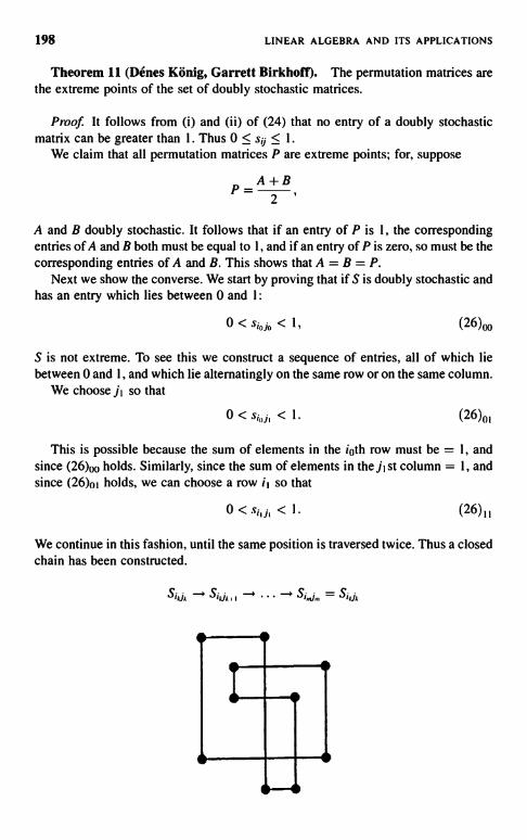
198 LINEAR ALGEBRA AND ITS APPLICATIONS
Theorem 11 (Denes Konig, Garrett Birkhoff). The permutation matrices arethe extreme points of the set of doubly stochastic matrices.
Proof. It follows from (i) and (ii) of (24) that no entry of a doubly stochasticmatrix can be greater than 1. Thus 0 < sy < 1.
We claim that all permutation matrices P are extreme points; for, suppose
A+BP_2 '
A and B doubly stochastic. It follows that if an entry of P is 1, the correspondingentries of A and B both must be equal to 1, and if an entry of P is zero, so must be thecorresponding entries of A and B. This shows that A = B = P.
Next we show the converse. We start by proving that if S is doubly stochastic andhas an entry which lies between 0 and 1:
0 < Sj' j' < 1, (26)00
S is not extreme. To see this we construct a sequence of entries, all of which liebetween 0 and 1, and which lie alternatingly on the same row or on the same column.
We choose ji so that
0 < si J, < 1. (26)01
This is possible because the sum of elements in the i0th row must be = 1, andsince (26)00 holds. Similarly, since the sum of elements in the j, st column = 1, andsince (26)01 holds, we can choose a row it so that
0<si,j,<1. (26)11
We continue in this fashion, until the same position is traversed twice. Thus a closedchain has been constructed.
CONVEXITY 199
We now define a matrix N as follows:(a) The entries of N are zero except for those points that lie on the chain.(b) The entries of N on the points of the chain are +I and -1, in succession.
The matrix N has the following property:(c) The row sums and column sums of N are zero.
We now define two matrices A, B by
A=S+EN, B=S-EN.
It follows from (c) that the row sums and columns sums of A and B are both 1. By (a)and the construction the elements of S are positive at all points where N has anonzero entry. It follows therefore that a can be chosen so small that both A and Bhave nonnegative entries. This shows that A and B both are doubly stochastic. SinceA # B, and
A+BS-
2 '
it follows that S is not an extreme point.It follows that extreme points of the set of doubly stochastic matrices have entries
either 0 or 1. It follows from (24) that each row and each column has exactly one 1. Itis easy to check that such a matrix is a permutation matrix. This completes the proofof the converse.
Applying Theorem 10 in the situation described in Theorem U, we conclude:Every doubly stochastic matrix can be written as a convex combination ofpermutation matrices:
S=Ec(P)P, c(P)>0, >c(P)=1.
EXERCISE 19. Show that, except for two dimensions, the representation ofdoubly stochastic matrices as convex combinations of permutation matrices is notunique.
Caratheodory's theorem has many applications in analysis. Its infinite-dimensional version is the Krein-Milman Theorem.
The last item in the chapter is a kind of a dual of Caratheodory's theorem.
Theorem 12 (Helly). Let X be a linear space of dimension n over the reals. Let{K1 .... , KN} be a collection of N convex sets in X. Suppose that every subcollectionof n + I sets K has a nonempty intersection. Then all K in the whole collection havea common point.

200 LINEAR ALGEBRA AND ITS APPLICATIONS
Proof (Radon). We argue by induction on N, the number of sets, starting with thetrivial situation N = n + 1. Suppose that N > n + I and that the assertion is true forN - l sets. It follows that if we omit any one of the sets, say Ki, the rest have a pointxi in common:
xi E Kj, j # i. (27)
We claim that there are numbers a,. .. , aN, not all zero, such that
and
N
Ea,=0.
(28)
(28)'
These represent n + 1 equations for the N unknowns. According to Corollary A'(concrete version) of Theorem I of Chapter 3, a homogeneous system of linearequations has a nontrivial (i.e., not all unknowns are equal to 0) solution if thenumber of equations is less than the number of unknowns. Since in our case n + I isless than N, (28) and (28)' have a nontrivial solution.
It follows from (28)' that not all ai can be of the same sign; there must be somepositive ones and some negative ones. Let us renumber them so that ai...... a,, arepositive, the rest nonpositive.
We define a by
Paai. (29)
Note that it follows from (28)' that
N
a= - Eai. (29)'P+1
We define y by
1 P
)' = Q E aix,. (30)
Note that it follows from (28) and (30) that
1
N- aixi (30)'a P+i

CONVEXITY 201
Each of the points xi, i = 1, ... , p belongs to each of the sets K1, j > p. It followsfrom (29) that (30) represents y as a convex combination of xj, ... , xp. Since ICJ isconvex, it follows that y belongs to K1 for j > p.
On the other hand, each xi, i = p + I,.. . , N belongs to each K j < p. It followsfrom (29)' that (30)' represents y as a convex combination of xi,+i,... ,xv. Since KKis convex, it follows that y belongs to KJ for j < p. This concludes the proof ofHelly's theorem. 0
Remark. Helly's theorem is nontrivial even in the one-dimensional case. Hereeach Kj is an interval, and the hypothesis that every Kj and K; intersects implies thatthe lower endpoint a; of any K; is less than or equal to the upper endpoint bj of anyother Kj. The point in common to all is then sup ai or inf b,, or anything in between.
Remark. In this chapter we have defined the notions of open convex set, closedconvex set, and bounded convex set purely in terms of the linear structure of thespace containing the convex set. Of course the notions open, closed, bounded have ausual topological meaning in terms of the Euclidean distance. It is easy to see that ifa convex set is open, closed, or bounded in the topological sense, then it is open,closed, or bounded in the linear sense used in this chapter.
EXERCISE 20. Show that if a convex set in a finite-dimensional Euclidean spaceis open, or closed, or bounded in the linear sense defined above, then it is open, orclosed, or bounded in the topological sense, and conversely.
CHAPTER 13
The Duality Theorem
Let X be a linear space over the reals, dim X = n. Its dual X' consists of all linearfunctions on X. If X is represented by column vectors x of n components x1,.. . , xn,
then elements of X' are traditionally represented as row vectors with n componentst , ... , in. The value of at x is
Ix1 + ... + Snxn. (1)
If we regard as a 1 x n matrix and regard x as an n x 1 matrix, (1) is their matrixproduct lx.
Let Y be a subspace of X; in Chapter 2 we have defined the annihilator Y1 of Yasthe set of all linear functions t; that vanish on Y, that is, satisfy
ty = 0 for all y in Y. (2)
According to Theorem 3 of Chapter 2, the dual of X' is X itself, and according toTheorem 5 there, the annihilator of Y1 is Y itself. In words: if tx = O for all in Y1,then x belongs to Y.
Suppose Yis defined as the linear space spanned by m given vectors yi,... ,yn inX. That is, Y consists of all vectors y of the form
(3)
Clearly, l; belongs to Y1 iff
Yj = 0, j = 1,..., M. (4)
Linear Algebra and Its Applications, Second Edition, by Peter D. LaxCopyright Q 2007 John Wiley & Sons, Inc.
202
THE DUALITY THEOREM 203
So for the space Ydefined by (3), the duality criterion stated above can be formulatedas follows: a vector y can be written as a linear combination (3) of in given vectors yjiff every that satisfies (4) also satisfies t y = 0.
We are asking now for a criterion that a vector y be the linear combination of mgiven vectors yj with nonnegative coefficients:
y = > PjYi, Pi?0. (5)
Theorem 1 (Farkas-Minkowski). A vector y can be written as a linearcombination of given vectors yj with nonnegative coefficients as in (5) iff every thatsatisfies
yj ? 0, j= (6)
also satisfies
ty ? 0.(6)'
Proof. The necessity of condition (6)' is evident upon multiplying (5) on the leftby i. To show the sufficiency we consider the set K of all points y of form (5). Clearly,this is a convex set; we claim it is closed. To see this we first note that any vector ywhich may be represented in form (5) may be represented so in various ways.Among all these representations there is by local compactness one, or several, forwhich E pj is as small as possible. We call such a representation of y a minimalrepresentation.
Now let {z,,} be a sequence of points of K converging to the limit z in theEuclidean norm. Represent each z minimally:
Z. = E pn.jyj. (5)'
We claim that E p,,, j = P is a bounded sequence. For suppose on the contrary thatP -> oo. Since the sequence z is convergent, it is bounded; therefore tends tozero:
Zn _ Pn.iyJ 0.
Pn P.
The numbers pn, j/P are nonnegative and their sum is 1. Therefore by compactnesswe can select a subsequence for which they converge to limits:
Pn.j' 9j-
P11
204 LINEAR ALGEBRA AND ITS APPLICATIONS
These limits satisfy > qj = 1. It follows from (5)" that
E gjyi = 0.
Subtract this from (5)':
For each j for which qj > 0, pn.j oo; therefore for n large enough, this is a positiverepresentation of z,,, showing that (5)' is not a minimal representation. Thiscontradiction shows that the sequence Pn = E p,, j is bounded. But then by localcompactness we can select a subsequence for which p,, ,j -> pj for all j. Let n tend tooc in (5)'; we obtain
z = limz = >P,)'j
Thus the limit z can be represented in the form (5); this proves that the set K of allpoints of form (5) is closed in the Euclidean norm.
We note that the origin belongs to K.Let y be a vector that does not belong to K. Since K is closed and convex,
according to the hyperplane separation Theorem 7 of Chapter 12 there is a closedhalfspace
(7)
that contains K but not y:
ny < c. (8)
Since 0 belongs to K, it follows from (7) that 0 > c. Combining this with (8), we get
ny<0.
Since kyj belongs to K for any positive constant k, it follows from (7) that
kr1Yj > c, j = l.... , in
for all k > 0; this is the case only if
l1)y>0, j=1,...,m.
(9)
(10)
Thus if y is not of form (5), there is an q that according to (10) satisfies (6) butaccording to (9) violates (6)'. This completes the proof of Theorem 1. 0
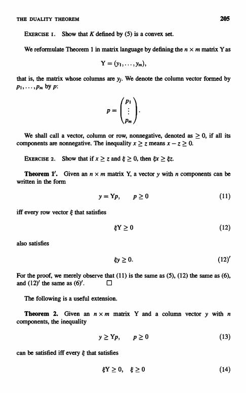
THE DUALITY THEOREM 205
EXERCISE I. Show that K defined by (5) is a convex set.
We reformulate Theorem 1 in matrix language by defining the n x m matrix Y as
y = (yI) ...,ym),
that is, the matrix whose columns are y,. We denote the column vector formed byPh,...,Pm by P:
We shall call a vector, column or row, nonnegative, denoted as > 0, if all itscomponents are nonnegative. The inequality x > z means x - z >_ 0.
EXERCISE 2. Show that if x > z and > 0, then i x > z.
Theorem 1. Given an n x m matrix Y, a vector y with n components can bewritten in the form
y=YP, P>-0 (11)
t th t ti fiif every row vec a sa s esor
Y > 0 (12)
also satisfies
y>_0. (12)'
For the proof, we merely observe that (11) is the same as (5), (12) the same as (6),and (12)' the same as (6)'.
The following is a useful extension.
Theorem 2. Given an n x m matrix Y and a column vectorcomponents, the inequality
y with n
y>YP, P>0 (13)
can be satisfied if every that satisfies
4Y>0, 4>0 (14)

206 LINEAR ALGEBRA AND ITS APPLICATIONS
also satisfies
by>_ 0. (15)
Proof. To prove necessity, multiply (13) by on the left and use (14) to deduce(15). Conversely by definition of > 0 for vectors, (13) means that there is a columnvector z with n components such that
y=Yp+z, z>_0, p>0. (13)'
We can rewrite (13)' by introducing the n x n identity matrix I, the augmented
matrix (Y, 1) and the augmented vector (p ). In terms of these (13)' can be written asz
y=(Y,I)(P), (P) >0(13)"
and (14) can be written as
(Y,I) > 0. (14)'
We now apply Theorem 1' to the augmented matrix and vector to deduce that if(15) is satisfied whenever (14)' is, then (13)" has a solution, as asserted inTheorem 2. O
Theorem 3 (Duality Theorem). Let Y be a given n x m matrix, y a givencolumn vector with n components, and y a given row vector with m components.
We define two quantities, S and s, as follows:
Definition
S = sup ypP
for all column vectors p with m components satisfying
(16)
y>YP, P>_0.
We call the set of p satisfying (17) admissible for the sup problem (16).
Definition
(17)
s = inf:y (18)
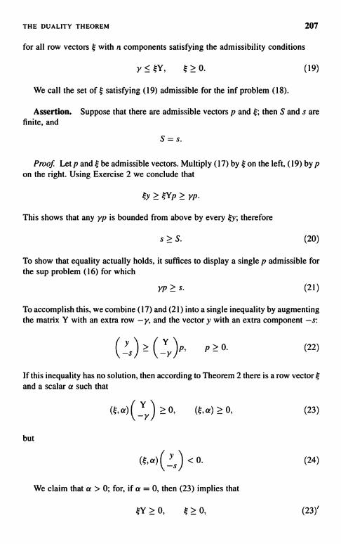
THE DUALITY THEOREM 207
for all row vectors with n components satisfying the admissibility conditions
y :5 4Y, > 0. (19)
We call the set of i satisfying (19) admissible for the inf problem (18).
Assertion. Suppose that there are admissible vectors p and ; then S and s arefinite, and
S=s.
Proof Let p and s; be admissible vectors. Multiply (17) by i on the left, (19) by pon the right. Using Exercise 2 we conclude that
y?.Yp?Yp
This shows that any yp is bounded from above by every y; therefore
s > S. (20)
To show that equality actually holds, it suffices to display a single p admissible forthe sup problem (16) for which
yp>s. (21)
To accomplish this, we combine (17) and (21) into a single inequality by augmentingthe matrix Y with an extra row -y, and the vector ), with an extra component -s:
C s J ? ( y)P, p > 0. (22)
If this inequality has no solution, then according to Theorem 2 there is a row vectorand a scalar a such that
(4,a)(YY) > 0, (,a) ? 0,
but
(23)
(, a) I ys < 0. (24)
We claim that a > 0; for, if a = 0, then (23) implies that
Y>0, >0, (23)'

208 LINEAR ALGEBRA AND ITS APPLICATIONS
and (24) that
iy < 0. (24)'
According to the "only if" part of Theorem 2 this shows that (13), the same as (17),cannot be satisfied; this means that there is no admissible p, contrary to assumption.
Having shown that a is necessarily positive, we may, because of the homogeneityof (23) and (24), take a = 1. Writing out these inequalities gives
Y >_ Y, ? 0 (25)
and
ty < S. (26)
Inequality (25), the same as (19), shows that is admissible; (26) shows that s isnot the infimum (18), a contradiction we got into by denying that we can satisfy (21).Therefore (21) can be satisfied; this implies that equality holds in (20). This provesthatS=s.
EXERCISE 3. Show that the sup and inf in Theorem 3 is a maximum andminimum. [Hint: The sign of equality holds in (21).]
We give now an application of the duality theorem in economics.We are keeping track of n different kinds of food (milk, meat, fruit, bread, etc.)
and m different kinds of nutrients (protein, fat, carbohydrates, vitamins, etc.). Wedenote
yU = number of units of the jth nutrient present in one unit of the ith food item.yj = minimum daily requirement of the jth nutrient.yi = price of one unit of the ith food item.
Note that all these quantities are nonnegative.Suppose our daily food purchase consists of ii units of the ith food item. We insist
on satisfying all the daily minimum requirements:
iyij >_ Y', j = 1, ... , m. (27)
This inequality can be satisfied, provided that each nutrient is present in at least oneof the foods.
The total cost of the purchase is
'iyi (28)

THE DUALITY THEOREM 209
A natural question is, What is the minimal cost of food that satisfies the dailyminimum requirements? Clearly, this is the minimum of (28) subject to (27) andl; > 0, since we cannot purchase negative amounts. If we identify the column vectorformed by the yi with y, the row vector formed by the yi with y, and the matrix yiiwith Y, the quantity (28) to be minimized is the same as (18), and (27) is the same as(19). Thus the infimum s in the duality theorem can in this model be identified withminimum cost.
To arrive at an interpretation of the supremum S we denote by {pi} a possible setof values for the nutrients that is consistent with the prices. That is, we require that
)'iyiipir i = 1,...,n. (29)
The value of the minimum daily requirement is
T, yipi' (30)
Since clearly pi are nonnegative, the restriction (29) is the same as (17). The quantity(30) is the same as that maximized in (16). Thus the quantity Sin the duality theoremis the largest possible value of the total daily requirement, consistent with the prices.
A second application comes from game theory. We consider two-person,deterministic, zero-sum games. Such a game can (by definition) always be presentedas a matrix game, defined as follows:
Ann x m matrix Y, called the payoff matrix, is given. The game consists of playerC picking one of the columns and player R picking one of the rows; neither playerknows what the other has picked but both are familiar with the payoff matrix. If Cchooses column j and R chooses row i, then the outcome of the game is the paymentof the amount Yii by player C to player R. If Yii is a negative number, then R pays C.
We think of this game as being played repeatedly many times. Furthermore, theplayers do not employ the same strategy each time, that is, do not pick the same row,respectively, column, each time, but employ a so-called mixed strategy whichconsists of picking rows, respectively columns, at random but according to a set offrequencies which each player is free to choose. That is, player C will choose the jthcolumn with frequency xi, where x is a probability vector, that is,
xi>0, > x1=1. (31)
iPlayer R will choose the ith row with frequency rii,
lii J 0, (31)'
Since the choices are made at random, the choices of C and R are independent ofeach other. It follows that the frequency with which C chooses column j and Rchooses row i in the same game is the product nixi.
210 LINEAR ALGEBRA AND ITS APPLICATIONS
Since the payoff of C to R is Y;1, the average payoff over a long time is
E rl;xjY+1.i.i
In vector-matrix notation that is
rjYx. (32)
If C has picked his mix x of strategies, then by observing over a long time R candetermine the relative frequencies that C is using, and therefore will choose his ownmix n of strategies so that he maximizes his gain:
max rjYx. (33)I?
Suppose C is a conservative player, that is, C anticipates that R will adjust his mix soas to gain the maximum amount (33). Since R's gain is Cs loss, C chooses his mix xto minimize his loss-that is, so that (33) is a minimum:
min max riYx,x q
(34)
x and q probability vectors.If, on the other hand, we suppose that R is the conservative player, R will assume
that C will guess R's mix n first and therefore C will choose x so that C's loss isminimized:
min rlYx.X
R therefore picks his mix q so that the outcome (33)' is as large as possible:
max min rlYx.1I X
(33)'
(34)'
Theorem 4 (Minmax Theorem). The minmax (34) and the maxmin (34)',where n and x are required to be probability vectors, are equal:
min max rjYx = max min r)Yx.x 11 q X
The quantity (35) is called the value of the matrix game Y.
(35)
Proof. Denote by E then x m matrix of all Is. For any pair of probability vectorsi and x, rl Ex = 1. Therefore if we replace Y by Y + kE, we merely add k to both (34)and (34)'. For k large enough all entries of Y + kE are positive; so we may consideronly matrices Y with all positive entries.

THE DUALITY THEOREM
We shall apply the duality theorem with
Y = (1,...,1)
Since y is positive, the maximum problem
211
(36)
S = max yp, y > Yp,p > 0 (37)P
has positive admissible vectors p. Since the entries of y are positive, S > 0. Wedenote by po a vector where the maximum is achieved.
Since Y > 0, the minimum problem
s=minty, tY?Y,4?0,4
(37)'
has admissible vectors . We denote by to a vector where the minimum is reached.According to (36), all components of y are 1; therefore ypo is the sum of the
components of po. Since ypo = S,
P0_xo _S
(38)
is a probability vector. Using an analogous argument, we deduce that
40 'no =s
(38)
is a probability vector.We claim that x0 and 'm are solutions of the minmax and maxmin problems (34)
and (34)', respectively. To see this, set po into the second part of (37), and divide byS. Using the definition xo = po/S, we get
y > Y.ro.S- (39)
Multiply this on the left with any probability vector n. Since according to (36) allcomponents of y are 1, ny = 1, and so
S > rlYxo. (40)
It follows from this that
1 > max r1Yxo,S- n

212 LINEAR ALGEBRA AND ITS APPLICATIONS
from which it follows that
I> min max riYx.
S x q
On the other hand, we deduce from (40) that for all q,
I> min iYx,S- x
from which it follows that
I > max min qYx.S- i x
(41)
(42)
Similarly we set a for into the second part of (37)', divide by s, and multiply byany probability vector x. By definition (38)', rin = 0/s; since according to (36) allcomponents of y are 1, yx = 1. So we get
r10Yx > 1 .
S
From this we deduce that for any probability vector x,
Imax rlYx > -I
n S
from which it follows that
1
min max rjYx > -.x n S
On the other hand, it follows from (40)' that
min g0Yx > 1X S
from which it follows that
max min ,Yx > I .
q x S
Since by the duality theorem S = s, (41) and (41)' together show that
(40)'
(41)'
(42)'
min maxiYx=1
=1-,
x ,i S S
THE DUALITY THEOREM
while (42) and (42)' show that
max min qYx =l l
S S
This proves the minmax theorem. El
213
The minmax theorem is due to von Neumann. It has important implications foreconomic theory.

CHAPTER 14
Nonmed Linear Spaces
In Chapter 12, Theorem 2, we saw that every open, convex set K in a linear space Xover R containing the origin can be described as the set of vectors x satisfyingp(x) < 1, where p, the gauge function of K, is a subadditive, positive homogeneousfunction, positive except at the origin. Here we consider such functions with oneadditional property: evenness, that is, p(-x) = p(x). Such a function is called anorm, and is denoted by the symbol jxI, the same as absolute value. We list now theproperties of a norm:
(i) Positivity: IxI > 0 forx 0 0, 101 = 0.(ii) Subadditivity: Ix+A 5 IxI + 1y1. (1)
(ill) Homogeneity: for any real numberk, jkxj = jkjjxj.
A linear space with a norm is called a normed linear space. Except for Theorem4, in this chapter X denotes a finite-dimensional normed linear space.
Definition. The set of points x in X satisfying I x I < 1 is called the open unitball around the origin; the set lxi < I is called the closed unit ball.
EXERCISE I. (a) Show that the open and closed unit balls are convex.(b) Show that the open and closed unit balls are symmetric with respect to the
origin, that is, if x belongs to the unit ball, so does -x.
Definition. The distance of two vectors x and y in X is defined as
Linear Algebra and Its Applications, Second Edition, by Peter D. LaxCopyright Q 2007 John Wiley & Sons, Inc.
214

NORMED LINEAR SPACES 215
EXERCISE 2. Prove the triangle inequality, that is, for all x, y, z in X,
Ix - zl <- Ix - yl+ly - ZI. (2)
Definition. Given a point y and a positive number r, the set of x satisfyingix - yl < r is called the open ball of radius r, center y; it is denoted B(),, r).
Examples
X=68",
(a) Define
lxl,, = max jail. (3)iProperties (i) and (iii) are obvious; property (ii) is easy to show.
(b) Define Ix12 as the Euclidean norm:
IXl2 = (lajl2) I/2(4)
Properties (i) and (iii) are obvious; property (ii) was shown in Theorem 3 ofChapter 7.
(c) Define
IxII = E jail- (5)
EXERCISE 3. Prove that Ixl I defined by (5) has all three properties (1) of a norm.The next example includes the first three as special cases:
(d) p any real number, I < p; we define
I/p
IxII, = (E lailp) (6)
Theorem 1. Ixlt, defined by (6) is a norm, that is, it has properties (1).
Proof. Properties (i) and (iii) are obvious. To prove (ii), we need thefollowing: 0
Holder's Inequality. Let p and q be positive numbers that satisfy
(7)p q
216 LINEAR ALGEBRA AND ITS APPLICATIONS
Let (a,, ..-,a.) =x and (bl, .... y be two vectors; then
xy <_IxIp IYIq,
where the product xy is defined as
xy = E ajbj;
(8)
(9)
IxIp, IYIq are defined by (6). Equality in (8) holds iff Iajlp and Ibjl' are proportionaland sgn aj = sgn bj, j = l , ... , n.
EXERCISE 4. Prove or look up a proof of Holder's inequality.
Note. For p = q = 2, Holder's inequality is the Schwarz inequality (see Theorem 1,Chapter 7).
EXERCISE 5. Prove that
where Ixlx is defined by (3).
Ixlx = slim Ixl p,
Corollary. For any vector x
IxIp=maxxy (10)
Proof. Inequality (8) shows that when lylq = 1, xy cannot exceed IxIp. Thereforeto prove (10) we have to exhibit a single vector yo, IYoiq = 1, for which Ayo = lxlp.Here it is:
Yo =
Clearly
and
z= (c1.... cj = sgnajlajlp/q (11)
I
IYoI =zlg
q lxlplq'P
Iz1qIcjlqIajlp=IxIp.Combining (12) and (12)'
IxIP/q
IYOI-q IxIP/q - 1.
P
zIxIplq '
P
(12)
(12)'
(13)
NORMED LINEAR SPACES
From (11)
217
xZ_yIajllajlplv_EIajI1+PIv
rrly (13)'x3o =IXIP/v
= IxiPIv - Ix1PIq = IXIP = IxIP,P P P
where we have used (7) to set 1 + p/q = p. Formulas (13) and (13)' complete theproof of the corollary.
To prove subadditivity for IxIP we use the corollary. Let x and z be any twovectors; then by (10),
Ix + zIP = max (x + z)y < max xy + max zy = IxIP + IzIP"1w=1 IYIq=1
This proves that the lP norm is subadditive.
We return now to arbitrary norms.
Definition. Two norms in a finite-dimensional linear space X, IXI I and IxI,, arecalled equivalent if there is a constant c such that for all x in X,
1X11 < CIXI2, IXI2 <_ cIXI I (14)
Theorem 2. In a finite-dimensional linear space, all norms are equivalent; thatis, any two satisfy (14) with some c, depending on the pair of norms.
Proof. Any finite-dimensional linear space X over IIB is isomorphic to R",n = dim X; so we may take X to be R". In Chapter 7 we introduced the Euclideannorm:
1/2
=(al,...,a,,). (15)IIXII= (EaJ) x
Denote by ej the unit vectors in 118":
ej = (0,...,1,0,...,0), j= 1,...,n.
Then x = (aI,...,a") can be written as
x = E ajej. (16)
Let IXI be any other norm in I. Using subadditivity and homogeneity repeatedlywe get
IXI < E Iajllejj. (16)'
218 LINEAR ALGEBRA AND ITS APPLICATIONS
Applying the Schwarz inequality to (16)' (see Theorem 1, Chapter 7), we get, using(15),
Ixl s:
(Ieji2)1 za,)i z-cllxll,(17)
where c abbreviates (E le 12) 112. This gives one half of inequalities (14).To get the other half, we show first that IxI is a continuous function with respect to
the Euclidean distance. By subadditivity,
IxI < Ix - yl + lyl, lyl <- Ix - yl + IxI,
from which we deduce that
Ilxl - 1Y11 :5 Ix -YI.
Using inequality (17), we get
IIXI - IYII<- cllx-yll,
which shows that IxI is a continuous function in the Euclidean norm.It was shown in Chapter 7 that the unit sphere Sin a finite-dimensional Euclidean
space, 11 x 11= 1, is a compact set. Therefore the continuous function IxI achieves itsminimum on S. Since by (1), IxI is positive at every point of S, it follows that theminimum m is positive. Thus we conclude that
0<m<Ix1 when 11x11=1.
Since both IxI and II x II are homogeneous functions, we conclude that
mllx11<_IxI
(18)
(19)
for all x in W. This proves the second half of the inequalities (14), and proves thatany norm in R" is equivalent in the sense of (14) with the Euclidean norm.
The notion of equivalence is transitive; if lxl, and 1x12 are both equivalent to theEuclidean norm, then they are equivalent to each other. This completes the proof ofTheorem 2.
Definition. A sequence {x"} in a normed linear space is called convergent tothe limit x, denoted as lim x" = x if lim lx" - xl = 0.
Obviously, the notion of convergence of sequences is the same with respect to twoequivalent norms; so by Theorem 2, it is the same for any two norms.
Definition. A set S in a normed linear space is called closed if it contains thelimits of all convergent sequences {x" }, x" in S.
NORMED LINEAR SPACES 219
ExERCISE 6. Prove that every subspace of a finite-dimensional normed linearspace is closed.
Definition. A set S in a nonmed linear space is called bounded if it is containedin some ball, that is, if there is an R such that for all points z in S, IzI _< R. Clearly, if aset is bounded in the sense of one norm, it is bounded in the sense of any equivalentnorm, and so by Theorem 2 for all norms.
Definition. A sequence of vectors {xk} in a normed linear space is called aCauchy sequence if Ixk - xj I tends to zero as k and j tend to infinity.
Theorem 3. (1) In a finite-dimensional normed linear space X, every Cauchysequence converges to a limit.
(ii) Every bounded infinite sequence in a finite-dimensional normed linearspace X has a convergent subsequence.
Property (i) of X is called completeness, and property (ii) is called localcompactness.
Proof. (i) Introduce a Euclidean structure in X. According to Theorem 2, theEuclidean norm and the norm in X are equivalent. Therefore a Cauchy sequence inthe norm of X is also a Cauchy sequence in the Euclidean norm. According toTheorem 16 in Chapter 7, a Cauchy sequence in a finite-dimensional Euclideanspace converges. But then the sequence also converges in the norm of X.
(ii) A sequence IX,} that is bounded in the norm of X is also bounded in theEuclidean norm imposed on X. According to Theorem 16 of Chapter 7, it contains asubsequence that converges in the Euclidean norm. But then that subsequence alsoconverges in the norm of X.
Just as in Euclidean space, see Theorem 17 in Chapter 7, part (ii) of Theorem 3has a converse:
Theorem 4. Let X be a normed linear space that is locally compact-that is, inwhich every bounded sequence has a convergent subsequence. Then X is finite-dimensional.
Proof. We need the following result.
Lemma 5. Let Y be a finite-dimensional subspace of a normed linear space X.Let x be a vector in X that does not belong to Y. Then
d = inf Ix - yjy in Y
is positive.

220 LINEAR ALGEBRA AND ITS APPLICATIONS
Proof. Suppose not; then there would be a sequence of vectors {y,, } in Y such that
0.
In words, y,, tends to x. It follows that {yn} is a Cauchy sequence; according to part(i) of Theorem 3, y converges to a limit in Y. This would show that the limit x of{y,, } belongs to Y, contrary to the choice of x.
Suppose X infinite-dimensional; we shall construct a sequence {yk} in X with thefollowing properties:
2, lyk - ytI ? 1 fork 1. (20)
Clearly, such a sequence is bounded and, equally clearly, contains no convergentsubsequence.
We shall construct the sequence recursively. Suppose have beenchosen; denote by Y the space spanned by them. Since X is infinite-dimensional,there is an x in X that does not belong to Y. We appeal now to Lemma 5,
d = inf Ix - yI > 0.vin Y
By definition of infimum, there is a vector yo in Y which satisfies
Ix - yol < 2d.
Define
Yn+i =x dyo(21)
It follows from the inequality above that I < 2. For any y in Y, yo + dy belongsto Y. Therefore by definition of infimum,
ix - yo - dye>d.
Dividing this by d and using the definition of y,,+,, we get
Iyn+I - yI > 1.
Since every yt, I = 1, ... , n, belongs to Y,
Iyn+i - y,I > 1 forl= I,...,n..
This completes the recursive construction of the sequence(20).
{yk} with property
Theorem 4 is due to Frederic Riesz.

NORMED LINEAR SPACES
EXERCISE 7. Show that the infimum in Lemma 5 is a minimum.
221
We have seen in Theorem 5 of Chapter 7 that every linear function I in aEuclidean space can be written in the form of a scalar product I(x) = (x, y).Therefore by the Schwarz inequality, Theorem I of Chapter 7,
II(x)I :5 IIx1IIIY II.
Combining this with (19), we deduce that
II(x)1 S clxl, c = II i II
We can restate this as Theorem 6.
Theorem 6. Let X be a finite-dimensional normed linear space, and let I be alinear function defined on X. Then there is a constant c such that
II(x)1 G clxl (22)
for all x in X.
Corollary 6. Every linear function on a finite-dimensional normed linear spaceis continuous.
Proof. Using the linearity of l and inequality (22), we deduce that
II(x) -1(y)I = II(x - y)I <- cIx - yI. O
Definition. Denote by co the infimum of all numbers c for which (22) holds forall x. Clearly, (22) holds for c = co, and co is the smallest number c for which (22)holds; co is called the norm of the linear function 1, denoted as III'.
The norm of l can also be characterized as
I IIII, = sup II()I (23)
It follows from (23) that for all x and all 1,
II(x)I <_ III'1x4. (24)
Theorem 7. X is a finite-dimensional normed linear space.
(i) Given a linear function I defined on X, there is an x in X, x # 0, for whichequality holds in (24).
(ii) Given a vector x in X, there is a linear function l defined on X, l # 0, forwhich equality holds in (24).

222 LINEAR ALGEBRA AND ITS APPLICATIONS
Proof. (i) We shall show that the supremum definition (23) of Ill' is a maximum.We note that the ratio I l (x) I /IxI doesn't change if we replace x by any multiple of x.Therefore it suffices to take the supremum (23) over the unit sphere IxI = 1.
According to Corollary 6', l(x) is a continuous function; then so is I1(x) I. Since thespace X is locally compact, the continuous function I1(x) I takes on its maximumvalue at some point x of the unit sphere. At this point, equality holds in (24).
(ii) If x = 0, any 1 will do.For x 9 0, we define 1(x) = IxI; since 1 is linear, we set for any scalar k
1(kx) = klxl. (25)
We appeal now to the Hahn-Banach Theorem, Theorem 4 in Chapter 12. We choosethe positive homogeneous, subadditive function p(x) to be IxI, and the subspace U onwhich 1 is defined consists of all multiples of x. It follows from (25) that for all u inU, 1(u) < Jul. According to Hahn-Banach, I can be extended to all y of X so that1(y) < IyI for all y. Setting -y for y, we deduce that I1(y)I < IyI as well. So bydefinition (23) of the norm of 1, it follows that Ill' < 1. Since 1(x) = IxI, it followsthat Ill' = 1, so equality holds in (24).
In Chapter 2 we have defined the dual of a finite-dimensional linear space X asthe set of all linear functions I defined on X. These functions form a linear space,denoted as X'. We have shown in Chapter 2 that the dual of X' can be identified withX itself: X" = X, as follows. For each x in X we define a linear function f over X' bysetting
Al) = 1(x). (26)
We have shown in Chapter 2 that these are all the linear functions on X.When X is a finite-dimensional nonmed linear space, there is an induced norm 111'
in X', defined by formula (23). This, in turn, induces a norm in the dual X" of V.
Theorem 8. The norm induced in X" by the induced norm in X' is the same asthe original norm in X.
Proof. The norm of a linear function of on X' is, according to formula (23),
IfI" = sup If(1)Ir,'o 111'
The linear functions f on X' are of the form (26); setting this into (27) gives
VI " = supI1(x) I
r,&oIlI
(27)
(28)

NORMED LINEAR SPACES 223
According to (24), Il(x)i/i1I' < lxi for all 134 0. According to part (ii) of Theorem 7,equality holds for some 1. This proves that Ifs" = lxI.
EXERCISE 8. Show that Ill' defined by (23) satisfies all postulates for a normlisted in (1).
Note. The dual of an infinite-dimensional normed linear space X consists of alllinear functions on X that are bounded in the sense of (22). The induced norm on X' isdefined by (24). Theorem 7 holds in infinite-dimensional spaces.
The dual of X' is defined analogously. For each x in X, we can define a linearfunction f by formula (25);f is bounded and its bound equals Jxj. So f lies in X"; butfor many spaces X that are used in analysis, it is no longer true that all elements f inX" are of the form (26).
Part (ii) of Theorem 7 can be stated as follows:
jxl = max 1(x) (29)III =[
for every vector x.The following is an interesting generalization of (29).
Theorem 9. Let Z be a subspace of X, y any vector in X. The distance d(y, Z) ofy to Z is defined to be
d(y, z) = in Z Iy - zl. (30)
Then
d(y, Z) = max 1(y) (31)
over all t: in X' satisfying
111,:51, 1(z) = 0 for z in Z. (32)
Proof. By definition of distance, for any e > 0 there is a zo in Z such that
1y-zol <d(y,Z)+e. (33)
For any I satisfying (32) we get, using (33) that
1(y) = l(y) - I(zo) = l(y - zo) <- Illly - zol < d(y, Z) +
Since e > 0 is arbitrary, this shows that for all I satisfying (32).
1(y) <_ d(y, z). (34)

224 LINEAR ALGEBRA AND ITS APPLICATIONS
To show the opposite inequality we shall exhibit a linear function in satisfying (32),such that m(y) = d(y,z). Since for y in Z the result is trivial, we assume that thevector y does not belong to Z. We define the linear subspace U to consist of allvectors u of the form
u=Z+ky, z in Z, k any real number. (35)
We define the linear function m(u) in U by
m(u) = kd(),, Z). (36)
Obviously, m is zero for u in Z; it follows from (35), (36), and the definition (30) of dthat
m(u) < Jul for a in U. (37)
By Hahn-Banach we can extend m to all of X so that (37) holds for all x; then
lmi' < 1. (37)'
Clearly, in satisfies (32); on the other hand, we see by combining (35) and (36) that
m(y) = d (y, Z)
Since we have seen in (34) that 1(y) < d(y, Z) for all I satisfying (32), this completesthe proof of Theorem 9.
In Chapter 1 we have introduced the notion of the quotient of a linear space X byone of its subspaces Z. We recall the definition: two vectors x, and x2 in X arecongruent mod Z,
x, =-x2 mod Z
if x, - x2 belongs to Z. We saw that this is an equivalence relation, and therefore wecan partition the vectors in X into congruence classes {}. The set of congruenceclasses { } is denoted as X/Z and can be made into a linear space; all this is describedin Chapter 1. We note that the subspace Z is one of the congruence classes, whichserves as the zero element of the quotient space.
Suppose X is a normed linear space; we shall show that then there is a natural wayof making X/Z into a normed linear space, by defining the following norm for thecongruence classes:
If = inf lxJ, x E {}. (38)

NORMED LINEAR SPACES 225
Theorem 10. Definition (38) is a norm, that is, has all three properties (1).
Proof. Every member x of a given congruence class () can be described asx = xo - z, xo some vector in { }, z any vector in Z. We claim that property (i),positivity, holds: for {} # 0,
IN > 0. (38)'
Suppose on the contrary that I { } I = 0. In view of definition (38) this means that thereis a sequence x1 in { } such that
lim IX.iI = 0. (39)
Since all xj belong to the same class, they all can be written as
Xi=XO - zi, zj in Z.
Setting this into (39) we get
limIxo-z;I=0.
Since by Theorem 3 every linear subspace Z is closed, it follows that xo belongs to Z.But then every point xo - z in { } belongs to Z, and in fact J} = Z. But we saw earlierthat {} = Z is the zero element of XIZ. Since we have stipulated {} # 0, we have acontradiction, that we got into by assuming I I) I = 0.
Homogeneity is fairly obvious; we turn now to subaddivity: by definition (38) wecan, given any E > 0, choose xo and {x}and yo in {y} so that
Ix01 < I{x}I + E, Iyo1 < I{y}I + E. (40)
Addition of classes is defined so that xo + yo belongs to {x} + {y}. Therefore bydefinition (38), subadditivity of I I and (39, 40),
I {x} + {y} I < Ixo + yol <- IxoI + 1yol < I {x} I + I {y} I + 2E.
Since f is an arbitrary positive number,
I{x} + {y}I < I{x}I + I{y}I
follows. This completes the proof of Theorem 10.
We conclude this chapter by remarking that a norm in a linear space over thecomplex numbers is defined entirely analogously, by the three properties (1). Thetheorems proved in the real case extend to the complex. To prove Theorems 7 and 9in the complex case, we need a complex version of the Hahn-Banach theorem, dueto Bohnenblust-Szobcyk and Sukhomlinov. Here it is:

226 LINEAR ALGEBRA AND ITS APPLICATIONS
Theorem 11. X is a linear space over C, and p is a real-valued function definedon X with the following properties:
(i) p is absolute homogeneous; that is, it satisfies
p(ax) = Ialp(x)
for all complex numbers a and all x in X.(ii) p is subadditive:
p(x + Y) < p(x) + p(Y)
Let U be a subspace of X, and I is a linear functional defined on U that satisfies
Il(u)I 5 P(u) (41)
for all u in U.Then I can be extended as a linear functional to the whole space so that
Il(x)I < p(x) (41)'
for all x in X.
Proof. The complex linear space X can also be regarded as a linear space over 08.Any linear function on complex X can be split into its real and imaginary part:
1(u) = 11(u) + il2(u),
where 11 and /2 are real-valued, and linear on real U. li and 12 are related by
h (iu) = -12(u).
Conversely, if 11 is a real-valued linear function over real X,
1(x) = 11W - ill (ix) (42)
is linear over complex X.We turn now to the task of extending 1. It follows from (41) that l1, the real part of
1, satisfies on U the inequality
11(u) < p(u). (43)
Therefore, by the real Hahn-Banach Theorem, /i can be extended to all of X sothat the extended / is linear on real X and satisfies inequality (43). Define l by
NORMED LINEAR SPACES 227
formula (42); clearly, it is linear over complex X and is an extension of I defined onU. We claim that it satisfies (41)' for all x in X. To see this, we factor l(x) as
l(x) = ar, r real, Ial = 1.
Using the fact that if 1(y) is real, it is equal to 11(y), we deduce that
Il(x)I = r =a-'l(x) = 1(a 'x) = !(a-'x) 5 p(a_'x)
= p(x). LI
We conclude this chapter by a curious characterization of Euclidean normsamong all norms. According to equation (53) of Chapter 7, every pair of vectors u, vin a Euclidean space satisfies the following identity:
IIu+v1I22+II U-VII2=2II u1I2+2II v1I2-
Theorem 12. This identity characterizes Euclidean space. That is, if in a realnormed linear space X
Iu + v12 + Iu - v12 = 2Iu12 +2 IV12
for all pairs of vectors u, v, then the norm II
is Euclidean.
Proof. We define a scalar product in X as follows:
4(x,y) = Ix +y12 - Ix - y12.
(44)
(45)
The following properties of a scalar product follow immediately from definition(45):
2 ,(x,x) = Ix1
Symmetry:
(46)
(Y,x) _ (x,Y),
and
(47)
(x, -Y) _ -(x,Y)
Next we show that (x, y) as defined in (45) is additive:
(48)
(x + Z! Y) = (x, y) + (z,y).
By definition (45),
(49)
4(x+z,y) = Ix+z+yI2- Ix+z- yI2. (50)

228 LINEAR ALGEBRA AND ITS APPLICATIONS
We apply now identity (44) four times:
(i) u=x+y,v'=z:
IX +y+z12+Ix+y-z12=21x+y1-+21z12 (SO)i
(ii) u=y+z, v=x:
Ix+y+z12+ly+z-x122=21y+z12+21x12 (51)jj
(iii) u = x - y, v = z:
Ix-y+z12+Ix-y-z12 = 21x-y12+21z12 (51);,,
(iv) u=z - y, v =x:
Iz-y+x12+ lz-y-x12 = 21z-y12+21x12 (51)j,
Add (51), and (51)ii, and subtract from it (51)iii and (51)j,; we get, after dividingby 2,
Ix+y+z12-Ix-y+z12= Ix + y12 - Ix - yl2 + ly + z12 - ly - z12.
(52)
The left-hand side of (52) equals 4(x + z, y), and the right-hand side is4(x, y) + 4(z, y). This proves (49).
EXERCISE 9. (i) Show that for all rational r,
(rx,y) = r(x,y).
(ii) Show that for all real k,
(kx,y) = k(x,y)

CHAPTER 15
Linear Mappings Between NormedLinear Spaces
Let X and Y be a pair of finite-dimensional nonmed linear spaces over the reals; weshall denote the norm in both spaces by I I, although they have nothing to do witheach other. The first lemma shows that every linear map of one nonmed linear spaceinto another is bounded.
Lemma 1. For any linear map T: X -+ Y, there is a constant c such that for all xin X,
ITxi < clxl. (1)
Proof. Express x with respect to a basis {xf }:
x=>aixj; (2)
then
By properties of the norm in Y,
From this we deduce that
Tx=>ajTxj.
ITxl laillTxll
ITxi < klxl., 3)
Linear Algebra and Its Applications, Second Edition, by Peter D. LaxCopyright Q 2007 John Wiley & Sons, Inc.
229
230
where
LINEAR ALGEBRA AND ITS APPLICATIONS
Ixlx = maxlail, k = ITxil.
We have noted in Chapter 14 that I Ix is a norm. Since we have shown in Chapter 14,Theorem 2, that all norms are equivalent, IxI, < const IxI and (1) follows from(3).
EXERCISE I. Show that every linear map T: X - Y is continuous, that is, if limx = x, then lim Tx,, = Tx.
In Chapter 7 we have defined the norm of a mapping of one Euclidean space intoanother. Analogously, we have the following definition.
Definition. The norm of the linear map T: X --> Y, denoted as ITI, is
ITI = supITxI
.
a-#0 IxI
Remark 1. It follows from (1) that ITI is finite.
(4)
Remark 2. It is easy to see that ITI is the smallest value we can choose for c ininequality (1).
Because of the homogeneity of norms, definition (4) can be phrased as follows:
ITI = sup ITxI. (4)'jxl=1
Theorem 2. ITI as defined in (4) and (4)' is a norm in the linear space of alllinear mappings of X into Y.
Proof. Suppose T is nonzero; that means that for some vector xo y6 0, Tx0 0 0.Then by (4),
ITI >IT*Ixol
since the norms in X and Yare positive, the positivity of ITI follows.
LINEAR MAPPINGS BETWEEN NORMED LINEAR SPACES 231
To prove subadditivity we note, using (4)', that when S and T are two mappings ofX -r Y, then
IT+SI = sup I(T + S)xI < sup(ITxI+ ISxI)Ix1=' hl=1
sup ITxI + sup ISxI = ITI + ISI11=1 1x1=1
The crux of the argument is that the supremum of a function that is the sum of twoothers is less than or equal to the sum of the separate suprema of the two summands.
Homogeneity is obvious; this completes the proof of Theorem 2.
Given any mapping T from one linear space X into another Y, we explained inChapter 3 that there is another map, called the transpose of T and denoted as T,mapping Y, the dual of Y, into X', the dual of X. The defining relation between thetwo maps is given in equation (9) of Chapter 3:
(T'l, x) = (l, Tx), (5)
where x is any vector in X and 1 is any element of 1'. The scalar product on the right,(1, y), denotes the bilinear pairing of elements y of Yand I of Y. The scalar product(m, x) on the left is the bilinear pairing of elements x in X and m in X'. Relation (5)defines T'1 as an element of V. We have noted in Chapter 3 that (5) is a symmetricrelation between T and T' and that
T"=T, (6)
just as X" is X and Y" is Y.We have shown in Chapter 14 that there is a natural way of introducing a dual
norm in the dual X' of a normed linear space X, see Theorem 7; for m in X',
ImI' = sup(m,x). (7)
The dual norm for l in Y is defined similarly as sup(l, y), IyI = 1; from this definition,[see equation (24) of Chapter 14], it follows that
(I,Y) <_ III' IYI (8)
Theorem 3. Let T be a linear mapping from a normed linear space X intoanother normed linear space Y, T' its transpose, mapping Y into X. Then
IT'I = ITI, (9)
where X' and Y are equipped with the dual norms.

232 LINEAR ALGEBRA AND ITS APPLICATIONS
Proof. Apply definition (7) to m = VI:
IT'll' = sup(T'1,x).Ixl= I
Using definition (5) of the transpose, we can rewrite the right-hand side as
IT'll' = sup(l,Tx).I.CI= I
Using the estimate (8) on the right, with y = Tx, we get
IT'll' < sup Ill' ITxI.k.1=1
Using (4)' to estimate ITxI we deduce that
IT'll<_I/1'ITI.
By definition (4) of the norm of T', this implies
IT'I S ITI
We replace now T by T' in (10); we obtain
(10)
IT"IS
IT'I. (10),
According to (6), T" = T, and according to Theorem 8 of Chapter 14, the norms inX" and 1, the spaces between which T" acts, are the same as the norms in X and Y.This shows that IT"I = ITI; now we can combine (10) and (10)' to deduce (9). Thiscompletes the proof of Theorem 3.
Let T be a linear map of a linear space X into Y, S another linear map of Y intoanother linear space Z. Then, as remarked in Chapter 3, we can define the product STas the composite mapping of T followed by S.
Theorem 4. Suppose X, Y, and Z above are normed linear spaces; then
ISTI <_ ISIITI. (11)
Proof. By definition (4),
ISyI S ISIIYI, ITxI S ITIIxI (12)
LINEAR MAPPINGS BETWEEN NORMED LINEAR SPACES 233
Hence
Applying definition (4) to ST completes the proof of inequality (11).
We recall that a mapping T of one linear space X into another is called invertible if itmaps X onto Y, and is one-to-one. In this case T has an inverse, denoted as T-1.
In Chapter 7, Theorem 15, we have shown that if a mapping B of a Euclideanspace into itself doesn't differ too much from another mapping A that is invertible,then B, too, is invertible. We present now a straightforward extension of this result tonormed linear spaces.
Theorem 5. Let X and Ybe finite-dimensional normed linear spaces of the samedimension, and let T be a linear mapping of X into Y that is invertible. Let S beanother linear map of X into Y that does not differ too much from T in the sense that
IS - TI < k, k =1
IT-'I
Then S is invertible.
ISTxI < ISIITxI s ISIITIIxI. (13)
(14)
Proof. We have to show that S is one-to-one and onto. We show first that S isone-to-one. We argue indirectly; suppose that for xo # 0,
Then
Since T is invertible,
Sxo=0.
Txo = (T - S)xo.
xo = T-' (T - S)xo.
(15)
Using Theorem 4 and (14) and that Ixol > 0, we get
Ixol < IT-'I IT - SIIxoI < IT-i Iklxol = Ixol,
a contradiction; this shows that (15) is untenable and so S is one-to-one.According to Corollary B of Theorem I in Chapter 3, a mapping S of a
linear space X into another linear space of the same dimension that is one-to-oneis onto. Since we have shown that S is one-to-one, this completes the proof ofTheorem 5.
Theorem 5 holds for normed linear spaces that are not finite dimensional,provided that they are complete. Corollary B of Theorem 1 of Chapter 3 does not

234 LINEAR ALGEBRA AND ITS APPLICATIONS
hold in spaces of infinite dimension; therefore we need a different, more directargument to invert S. We now present such an argument. We start by recalling thenotion of convergence in a nonmed linear space applied to the space of linear maps.
Definition. Let X, Y be a pair of finite-dimensional normed linear spaces. Asequence {Tn} of linear maps of X into Y is said to converge to the linear map T,denoted as limn, Tn = T, if
lim ITn - TI = 0.n-oo
(16)
Theorem 6. Let X be a nonmed finite-dimensional linear space, R a linear mapof X into itself whose norm is less than 1:
IRI < 1. (17)
Then
S=I-R (18)
is invertible, and00
S-1 = E Rk (18),
0
Proof. Denote Eo Rk as T, and denote Tnx as yn. We claim that {y} is a Cauchysequence; that is, Iyn - y1I tends to zero as n and I tend to oo. To see this, we write
yn - y1 = Tnx - Ttx = E Rkx.j+1
By the triangle inequality
Iyn -y!I :5 E IRtxI (19)j+l
Using repeatedly the multiplicative property of the norm of operators, we concludethat
IRkI <- IRIk.
It follows that
IRkxI < IRtIIxI < IRIkIxI
Set this estimate into (19); we get
a
Iyn - YjI <- (>IRIk/
kI.+1
(20)

LINEAR MAPPINGS BETWEEN NORMED LINEAR SPACES 235
Since SRI is assumed to be less than one, the right-hand side of (20) tends to zero as nn
and j tend to oo. This shows that yn = Tnx = E R"x is a Cauchy sequence.0
According to Theorem 3 of Chapter 14, every Cauchy sequence in a finite-dimensional normed linear space has a limit. We define the mapping T as
Tx = lim Tnx.n-roo
(21)
We claim that T is the inverse of I - R. According to Exercise 1, the mapping I - Ris continuous; therefore it follows from (21) that
(I - R)Tx = lim (I - R)Tnxn-.oo
Since Tn = Rk,0
n
(I - R)Tnx = (I - R) E Rkx = x - R"+Ix.0
as n - oo, the left-hand side tends to (I - R) Tx and the right-hand side tends to x,this proves that T is the inverse of I - R. O
EXERCISE 2. Show that if for every x in X, ITnx - TxI tends to zero as n -, oo,then ITn - TI tends to zero.
EXERCISE 3. Show that Tn = E Rk converges to S-1 in the sense of definition (16).0
Theorem 6 is a special case of Theorem 5, with Y = X and T = I.
EXERCISE 4. Deduce Theorem 5 from Theorem 6 by factoring S = T + S - TasT[I-T''(S-T)].
EXERCISE 5. Show that Theorem 6 remains true if the hypothesis (17) isreplaced by the following hypothesis. For some positive integer m,
JR'"I < 1. (22)
EXERCISE 6. Take X = Y = R", and T: X -f X the matrix Take for thenorm lxi the maximum norm 1x1,0 defined by formula (3) of Chapter 14. Show thatthe norm ITI of the matrix (t;,), regarded as a mapping of X into X, is
ITS = max> Ityl. (23)1
236 LINEAR ALGEBRA AND ITS APPLICATIONS
EXERCISE 7. Take X to be P t normed by the maximum norm Ixlx, Y to be 08"normed by the 1-norm 1x1 i, defined by formulas (3) and (4) in Chapter 14. Show thatthe norm of the matrix (tit) regarded as a mapping of X into Y is bounded by
ITI <_ E Ir,3I.ij
EXERCISE 8. X is any finite-dimensional normed linear space over C, and T is alinear mapping of X into X. Denote by tt the eigenvalues of T, and denote by r (T) itsspectral radius:
r(T) = max Itjj.
(i) Show that ITI > r(T).(ii) Show that IT"I > r(T)".
(iii) Show, using Theorem 18 of Chapter 7, that
lim IT"II/" = r(T)."-x

CHAPTER 16
Positive Matrices
Definition. A real I x I matrix P is called entrywise positive if all its entries pij arepositive real numbers.
Caution: This notion of positivity, used only in this chapter, is not to be confusedwith self-adjoint matrices that are positive in the sense of Chapter 10.
Theorem 1 (Perron). Every positive matrix P has a dominant eigenvalue,denoted by X(P) which has the following properties:
(i) I (P) is positive and the associated eigenvector h has positive entries:
Ph = A(P)h, h > 0. (1)
(ii) X (P) is a simple eigenvalue.(iii) Every other eigenvalue x of P is less than x(P) in absolute value:
JJ < A(P). (2)
(iv) P has no other eigenvectorf with nonegative entries.
Proof. We recall from Chapter 13 that inequality between vectors in 1$" meansthat the inequality holds for all corresponding components. We denote by p(P) theset of all nonnegative numbers A for which there is a nonnegative vector x # 0 suchthat
Px>Ax, x>0.
Linear Algebra and Its Applications, Second Edition, by Peter D. LaxCopyright Q 2007 John Wiley & Sons, Inc.
(3)
237
238 LINEAR ALGEBRA AND ITS APPLICATIONS
Lemma 2. For P positive,
(i) p(P) is nonempty, and contains a positive number,(ii) p(P) is bounded,(iii) p(P) is closed.
Proof. Take any positive vector x; since P is positive, Px is a positive vector.Clearly, (3) will hold for A small enough positive; this proves (i) of the lemma.
Since both sides of (3) are linear in x, we can normalize x so that
ix = E xi = 1, 4 _ (1,...,1). (4)
Multiply (3) by on the left:
Px > Aix = A. (5)
Denote the largest component of iP by b; then b > iP. Setting this into (5) givesb > A; this proves part (ii) of the lemma.
To prove (iii), consider a sequence of A" in p(P); by definition there is acorresponding x # 0 such that (3) holds:
Pxn > An, xn. (6)
We might as well assume that the x are normalized by (4):
The set of nonnegative x normalized by (4) is a closed bounded set in 01" andtherefore compact. Thus a subsequence of x tends to a nonnegative x alsonormalized by (4), while A" tends to A. Passing to the limit of (6) shows that x, Asatisfy (3); therefore p(P) is closed. This proves part (iii) of the lemma. O
Having shown that p(P) is closed and bounded, it follows that it has a maximumAmax; by (i), Amax > 0. We shall show now that Amax is the dominant eigenvalue.
The first thing to show is that Amax is an eigenvalue. Since (3) is satisfied by Amax,there is a nonnegative vector h for which
Ph > Amaxh, h > 0, h # 0; (7)
we claim that equality holds in (7); for, suppose not, say in the kth component:
L p i j h j > Amaxhi, i O k
POSITIVE MATRICES 239
Define the vector x = h + eek, where e > 0 end ek has kth component equal to 1, allother components zero. Since P is positive, replacing h by x in (7) increases eachcomponent of the left-hand side: Px > Ph. But only the kth component of the right-hand side is increased when h is replaced by x. It follows therefore from (7)' that fore small enough positive,
Px > Amaxx. (8)
Since this is a strict inequality, we may replace X. by Amax + 8, S positive but sosmall that (8) still holds. This shows that Amax + S belongs to p(P), contrary to themaximal character of A. This proves that Amax is an eigenvalue of P and that thereis a corresponding eigenvector h that is nonnegative.
We claim now that the vector h is positive. For certainly, since P is positive andh > 0, it follows that Ph > 0. Since Ph = Amaxh, h > 0 follows. This proves part (i)of Theorem 1.
Next we show that X. is simple. We observe that all eigenvectors of P witheigenvalue Amax must be proportional to h; for if there were another eigenvector y nota multiple of h, then we could construct h + cy, c so chosen that h + cy > 0 but oneof the components of h + cy is zero. This contradicts our argument above that aneigenvector of P is nonnegative is in fact positive.
To complete the proof of (ii) we have to show that P has no generalizedeigenvectors for the eigenvalue Amax, that is, a vector y such that
PY = AmaxY + ch. (9)
By replacing y by -y if necessary we can make sure that c > 0; by replacing y byy + bh if necessary we can make sure that y is positive; it follows then from (9) andh > 0 that Py > Amaxy. But then for S small enough, greater than 0,
Py > (Amax + 8)y,
contrary to X. being the largest number in p(P).To show part (iii) of Theorem 1, let if be another eigenvalue of P, not equal
to Amax, y the corresponding eigenvector, both possibly complex: Py = icy;componentwise,
:Pijyj = KYii
Using the triangle inequality for complex numbers and their absolute values,we get
EPiuIYII ? PijYil = IKIIYil. (10)i i

240 LINEAR ALGEBRA AND ITS APPLICATIONS
Comparing this with (3), we see that IKI belongs to p(P). If IKI were = Amax, thevector
lyi I
ly'I
would be an eigenvector of P with eigenvalue Am., and thus proportional to h:
ly'I=chi. (11)
Furthermore, the sign of equality would hold in (10). It is well known about complexnumbers that this is the case only if all the yl have the same complex argument:
y'=e'ely;I, i= 1,...,1
Combining this with (11) we see that
y; = ceehi, that is, y = (ce'B)h.
Thus K = Am., and the proof of part (iii) is complete.To prove (iv) we recall from Chapter 6, Theorem 17, that the product of
eigenvectors of P and its transpose PT pertaining to different eigenvalues is zero.Since pT also is positive, the eigenvector pertaining to its dominant eigenvalue,which is the same as that of P, has positive entries. Since a positive vector 4 does notannihilate a nonnegative vector f, part (iv) follows from 4f = 0. This completes theproof of Theorem 1.
The above proof is due to Bohnenblust; see R. Bellman, Introduction to MatrixAnalysis.
EXERCISE I. Denote by t(P) the set of nonnegative A such that
Px<Ax, x>O
for some vector x # 0. Show that the dominant eigenvalue A(P) satisfies
A(P) = min A. (12))LE !(P)
We give now some applications of Perron's theorem.
Definition. A stochastic matrix is an I x I matrix S whose entries arenonnegative:
Sy>0, (13)
POSITIVE MATRICES 241
and whose column sums are equal to 1:
s;1=1, j=1,...,1. (14)
The interpretation lies in the study of collections of l species, each of which hasthe possibility of changing into another. The numbers sib are called transitionprobabilities; they represent the fraction of the population of the jth species that isreplaced by the ith species. Condition (13) is natural for this interpretation; condition(14) specifies that the total population is preserved. There are interestingapplications where this is not so.
The kind of species that can undergo change describable as in the foregoing areatomic nuclei, mutants sharing a common ecological environment, and many others.
We shall first study positive stochastic matrices, that is, ones for which (13) is astrict inequality. To these Perron's theorem is applicable and yields the followingtheorem.
Theorem 3. Let S be a positive stochastic matrix.
(i) The dominant eigenvalue k(S) = 1.(ii) Let x be any nonnegative vector; then
lim SNx = ch,N-x
where h the dominant eigenvector and c is some positive constant.
(15)
Proof. As remarked earlier, if S is a positive matrix, so is its transpose ST. Since,according to Theorem 16, Chapter 6, S and ST have the same eigenvalues, it followsthat S and ST have the same dominant eigenvalue. Now the dominant eigenvalue ofthe transpose of a stochastic matrix is easily computed: It follows from (14) that thevector with all entries 1,
= (1,..., 1).
is a left eigenvector of S, with eigenvalue 1. It follows from part (iv) Theorem 1 thatthis is the dominant eigenvector and 1 is the dominant eigenvalue. This proves part (i).
To prove (ii), we expand x as a sum of eigenvectors hh of S:
x = E cihl.
Assuming that all eigenvectors of S are genuine, not generalized, we get
SNX =
(16)
(16)N
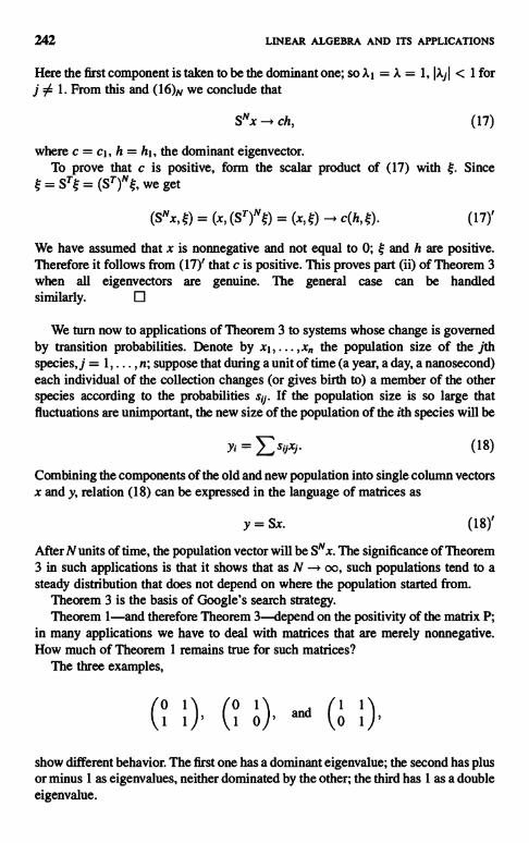
242 LINEAR ALGEBRA AND ITS APPLICATIONS
Here the first component is taken to be the dominant one; so.l1 = A = 1, jXj <I forj # 1. From this and (16)N we conclude that
SNx -> ch, (17)
where c = cl, h = hl, the dominant eigenvector.To prove that c is positive, form the scalar product of (17) with i;. Since
= ST = (ST we get
(SNx, ) = (x, (ST (x, ) - c(h, ) (17)'
We have assumed that x is nonnegative and not equal to 0; i and h are positive.Therefore it follows from (17)' that c is positive. This proves part (ii) of Theorem 3when all eigenvectors are genuine. The general case can be handledsimilarly.
We turn now to applications of Theorem 3 to systems whose change is governedby transition probabilities. Denote by x1,. .. , x the population size of the jthspecies, j = 1, . . . , n; suppose that during a unit of time (a year, a day, a nanosecond)each individual of the collection changes (or gives birth to) a member of the otherspecies according to the probabilities sy. If the population size is so large thatfluctuations are unimportant, the new size of the population of the ith species will be
Yi = Esgxj (18)
Combining the components of the old and new population into single column vectorsx and y, relation (18) can be expressed in the language of matrices as
y = Sx. (18)'
After N units of time, the population vector will be SNx. The significance of Theorem3 in such applications is that it shows that as N -+ oo, such populations tend to asteady distribution that does not depend on where the population started from.
Theorem 3 is the basis of Google's search strategy.Theorem 1-and therefore Theorem 3-depend on the positivity of the matrix P;
in many applications we have to deal with matrices that are merely nonnegative.How much of Theorem 1 remains true for such matrices?
The three examples,
(01)'
(1 10),and
(I0
1
),
show different behavior. The first one has a dominant eigenvalue; the second has plusor minus 1 as eigenvalues, neither dominated by the other; the third has I as a doubleeigenvalue.

POSITIVE MATRICES 243
EXERCISE 2. Show that if some power P' of P is positive, then P has a dominantpositive eigenvalue.
There are other interesting and useful criteria for nonnegative matrices to have adominant positive eigenvalue. These are combinatorial in nature; we shall not speakabout them. There is also the following result, due to Frobenius.
Theorem 4. Every nonnegative l x I matrix F, F 54 0, has an eigenvalue A(F)with the following properties:
(i) A(F) is nonnegative, and the associated eigenvector has nonnegative entries:
Fh = A(F)h, h > 0. (19)
(ii) Every other eigenvalue K is less than or equal to A(F) in absolute value:
SKI < A(F).
(iii) If SKI = A(F), then K is of the form
K = e27rik/mA(F)
where k and m are positive integers, m < 1.
(20)
(21)
Remark. Theorem 4 can be used to study the asymptotically periodic behaviorfor large N of S"x, where S is a nonnegative stochastic matrix. This has applicationsto the study of cycles in population growth.
Proof. Approximate F by a sequence F of positive matrices. Since thecharacteristic equations of F,, tend to the characteristic equations of F, it followsthat the eigenvalues of F,, tend to the eigenvalues of F. Now define
A(F) = lim k(F,,).n-.x
Clearly, as n oc, inequality (20) follows from inequality (2) for F,,. To prove (i),we use the dominant eigenvector hn of F,,, normalized as in (4):
hn = 1, = 0,..., 0.
By compactness, a subsequence of h,, converges to a limit vector h. Being the limitof normalized positive vectors, h is nonnegative. Each h,, satisfies an equation
Fnhn = A(F,,)hni
letting n tend to oo we obtain relation (19) in the limit.

244 LINEAR ALGEBRA AND ITS APPLICATIONS
Part (iii) is trivial when A(F) = 0; so we may assume A(F) > 0; at the cost ofmultiplying F by a constant we may assume that x(F) = 1. Let x be a complexeigenvalue of F, liJ = .l(F) = 1; then x can be written as
k=ei9. (22)
Denote by y + iz the corresponding eigenvector:
F(y + iz) = e'a (y + iz). (23)
Separate the real and imaginary parts:
Fy=cosBy-sin9z,(23)'
Fz=sin9z+cosBy.
The geometric interpretation of (23)' is that in the plane spanned by the vectors y andz, F is rotation around the origin by 9.
Consider now the plane formed by all points x of the form
x = h + ay + bz, (24)
a and b arbitrary real numbers, h the eigenvector (19). It follows from (19) and (23)'that in this plane F acts as rotation by 9. Consider now the set Q formed by allnonnegative vectors x of form (24); if Q contains an open subset of the plane (24), itis a polygon. Since F is a nonnegative matrix, it maps Q into itself; since it is arotation, it maps Q onto itself. Since Q has I vertices, the Ith power of F is theidentity; this shows that F rotates Q by an angle 9 = 2irk/l.
It is essential for this argument that Q be a polygon, that is, that it contain an openset of the plane (24). This will be the case when all components of h are positive orwhen some components of h are zero, but so are the corresponding components of yand z. For then all points x of form (24) with dal, IbI small enough belong to Q; in thiscase Q is a polygon.
To complete the proof of Theorem 4(iii), we turn to the case when somecomponents of h are zero but the corresponding components of y or z are not.Arrange the components in such an order that the first j components of h are zero, therest positive. Then it follows from Fh = h that F has the following block form:
F = (F0 B I. (25)
Denote by yo and zo the vectors formed by the first j components of y and z. Byassumption, yo + izo 0 0. Since by (23), y + iz is an eigenvector of F witheigenvalue 0, it follows from (25) that yo + izo is an eigenvector of FO:
Fo(yo + izo) = e'e(yo + izo).

POSITIVE MATRICES 245
Since Fo is a nonnegativej x j matrix, it follows from part (ii) of Theorem 4 alreadyestablished that the dominant eigenvalue A(Fo) cannot be less than Ie`°I = 1. Weclaim that equality holds: A(Fo) = 1. For, suppose not; then the correspondingeigenvector ho would satisfy
Foho = (1 + S)ho, ho > 0,S > 0. (26)
Denote by k the 1-vector whose first j components are those of ho, the rest are zero. Itfollows from (26) that
Fk > (1 + 8)k. (26)'
It is easy to show that the dominant eigenvalue A(F) of a nonnegative matrix can becharacterized as the largest .X for which (3) can be satisfied. Inequality (26)' wouldimply that A(F) > 1 +S, contrary to the normalization A(F) = 1. This proves thatA(Fo) = 1.
We do now an induction with respect to j on part (iii) of Theorem 4. Since e'0 is aneigenvalue of the j x j matrix FO, and A(Fo) = 1, and since j < 1, it follows by theinduction hypothesis that 0 is a rational multiple of 2,r with denominator less than orequal to j. This completes the proof of Theorem 4.
CHAPTER 17
How to Solve Systemsof Linear Equations
To get numerical answers out of any linear model, one must in the end obtain thesolution of a system of linear equations. To carry out this task efficiently hastherefore a high priority; it is not surprising that it has engaged the attention of someof the leading mathematicians. Two methods still in current use, Gaussianelimination and the Gauss-Seidel iteration, were devised by the Prince ofMathematicians. The great Jacobi invented an iterative method that bears his name.
The availability of programmable, high-performance computers with largememories-and remember, yesterday's high-performance computer is today'spocket computer-has opened the floodgates; the size and scope of linear equationsthat could be solved efficiently has been enlarged enormously and the role of linearmodels correspondingly enhanced. The success of this effort has been due not onlyto the huge increase in computational speed and in the size of rapid access memory,but in equal measure to new, sophisticated, mathematical methods for solving linearequations. At the time von Neumann was engaged in inventing and building aprogrammable electronic computer, he devoted much time to analyzing theaccumulation and amplification of round-off errors in Gaussian elimination. Othernotable early efforts were the very stable methods that Givens and Householderfound for reducing matrices to Jacobi form (see Chapter 18).
It is instructive to recall that in the 1940s linear algebra was dead as a subject forresearch; it was ready to be entombed in textbooks. Yet only a few years later, inresponse to the opportunities created by the availability of high-speed computers,very fast algorithms were found for the standard matrix operations that astoundedthose who thought there were no surprises left in this subject.
In this chapter we describe a few representative modern algorithms for solvinglinear equations. Included among them, in Section 4, is the conjugate gradientmethod developed by Lanczos, Stiefel, and Hestenes.
Linear Algebra and Its Applications. Second Edition, by Peter D. LaxCopyright r; 2007 John Wiley & Sons, Inc.
246

HOW TO SOLVE SYSTEMS OF LINEAR EQUATIONS 247
The systems of linear equations considered in this chapter are of the class thathave exactly one solution. Such a system can be written in the form
Ax = b, (1)
A an invertible square matrix, b some given vector, x the vector of unknowns to bedetermined.
An algorithm for solving the system (1) takes as its input the matrix A and thevector b and produces as output some approximation to the solution x. In designingand analyzing an algorithm we must first understand how fast and how accurately analgorithm works when all the arithmetic operations are carried out exactly. Second,we must understand the effect of rounding, inevitable in computers that do theirarithmetic with a finite number of digits.
With algorithms employing billions of operations, there is a very real danger thatround-off errors not only accumulate but are magnified in the course of thecalculation. Algorithms for which this does not happen are called arithmeticallystable.
It is important to point out that the use of finite digit arithmetic places an absolutelimitation on the accuracy with which the solution can be determined. To understandthis, imagine a change Sb being made in the vector b appearing on the right in (1).Denote by Sx the corresponding change in x:
A(x + Sx) = b + Sb.
since according to (1), Ax = b, we deduce that
ASx = Sb.
(2)
(3)
We shall compare the relative change in x with the relative change in b, that is, theratio
18X1 ISb1
IxI IbI '(4)
where the norm is convenient for the problem. The choice of relative change isnatural when the components of vectors are floating point numbers.
We rewrite (4) as
IbI ISxl _ IAxI IA-'SbI
IxI I SbI IxI ISbI(4)'
The sensitivity of problem (1) to changes in b is estimated by maximum of (4)' overall possible x and Sb. The maximum of the first factor on the right in (4)' is JAI, thenorm of A; the maximum of the second factor is IA-1 I, the norm of A-'. Thus we
248 LINEAR ALGEBRA AND ITS APPLICATIONS
conclude that the ratio (4) of the relative error in the solution x to the relative error inb can not be larger than
K(A) = IAI IA-' I. (5)
The quantity K(A) is called the condition number of the matrix A.
EXERCISE I. Show that K(A) is > 1.
Since in k-digit floating point arithmetic the relative error in b can be as large as10-'t, it follows that if equation (1) is solved using k-digit floating point arithmetic,the relative error in x can be as large as 10-kK(A).
It is not surprising that the larger the condition number K(A), the harder it is tosolve equation (1), for K(A) = oc when the matrix A is not invertible. As we shallshow later in this chapter, the rate of convergence of iterative methods to the exactsolution of (1) is slow when K(A) is large.
Denote by ,B the largest absolute value of the eigenvalues of A. Clearly,
fi 5 IAI. (6)
Denote by a the smallest absolute value of the eigenvalues of A. Then applyinginequality (6) to the matrix A-' we get
< IA-11. (6)'
Combining (6) and (6)' with (5) we obtain this lower bound for the condition numberof A:
(7)
An algorithm that, when all arithmetic operations are carried out exactly,furnishes in a finite number of steps the exact solution of (1) is called a directmethod. Gaussian elimination discussed in Chapter 4 is such a method. An algorithmthat generates a sequence of approximations that tend, if all arithmetic operationswere carried out exactly, to the exact solution is called an iterative method. In thischapter we shall investigate the convergence and rate of convergence of severaliterative methods.
Let us denote by the sequence of approximations generated by analgorithm. The deviation of x from x is called the error at the nth stage, and isdenoted by e,,:
e = x - x. (8)
HOW TO SOLVE SYSTEMS OF LINEAR EQUATIONS 249
The amount by which the nth approximation fails to satisfy equation (1) is called thenth residual, and is denoted by r,,:
Residual and error are related to each other by
r,, = Ae,,.
(9)
(10)
Note that, since we do not know x, we cannot calculate the errors en; but once wehave calculated x,, we can by formula (9) calculate r,,.
In what follows, we shall restrict our analysis to the case when the matrix A isreal, self-adjoint, and positive; see Chapter 8 and Chapter 10 for the definition ofthese concepts. We shall use the Euclidean norm, denoted as II II, to measure the sizeof vectors.
We denote by a and P the smallest and largest eigenvalues of A. Positivedefiniteness of A implies that a is positive, see Theorem I of Chapter 10. We recallfrom Chapter 8, Theorem 12, that the norm of a positive matrix with respect to theEuclidean norm is its largest eigenvalue;
IIAII=6. (11)
Since A-' also is positive, we conclude that
11 A-' II = a-'. (11)'
Recalling the definitions (5) of the condition number Awe conclude that for A self-adjoint and positive,
(12)
1. THE METHOD OF STEEPEST DESCENT
The first iterative method we investigate is based on the variational characterizationof the solution of equation (1) in the case when A is positive definite.
Theorem 1. The solution x of (1) minimizes the functional
E(y) =1(y, Ay) - (y, b); (13)
here (,) denotes the Euclidean scalar product of vectors.
Proof. We add to E(y) a constant, that is, a term independent of y:
F(y) = E(y) + 2(x, b). (14)

250
F(x) = 0.
Set (13) into (14); using Ax = b and the self-adjointness of A we can expressF(y) as
F(y) =i(y-x,A(y-x)). (14)'
Clearly,
A being positive means that (v, Av) > 0 for v # 0. Thus (14)' shows that F(y) > 0for y 54 x. This proves that F(y), and therefore E(y), takes on its minimum aty=x.
Theorem I shows that the task of solving (1) can be accomplished by minimizingE. To find the point where E assumes its minimum we shall use the method ofsteepest descent; that is, given an approximate minimizer y, we find a betterapproximation by moving from y to a new point along the direction of the negativegradient of if. The gradient of E is easily computed from formula (13):
grad E(y) = Ay - b.
So if our nth approximation is x,,, then the (n + I)st, x,,+,, is
xn+1 = xn - S(Axn - b), (15)
where s is step length in the direction -grad E. Using the concept (9) of residual, wecan rewrite (15) as
xx+1 = xn - Srn. (15)'
We determine s so that E(xn+1) is as small as possible. This quadratic minimumproblem is easily solved; using (13) and (9), we have
E(xn+1) = 2(xn - srn, A(xn - srn)) - (xn - srn, b)
= E(xn) - s(rn, rn) + 262(rn, Ar,,).
Its minimum is reached for
LINEAR ALGEBRA AND ITS APPLICATIONS
(rn, rn)n
(rn, Arn)s =
(15)"
(16)
Theorem 2. The sequence of approximations defined by (15), with s given by(16), converges to the solution x of (1).

HOW TO SOLVE SYSTEMS OF LINEAR EQUATIONS 251
Proof. We need a couple of inequalities. We recall from Chapter 8 that for anyvector r the Rayleigh quotient
(r, Ar)(r, r)
of a self-adjoint matrix A lies between the smallest and largest eigenvalues of A. Inour case these were denoted by a and 0; so we deduce from (16) that
1 1
We conclude similarly that for all vectors r,
1 (r,A-1r) I0-(r,
r) <a
(17)
(17)'
We show now that F(x,,) tends to zero as n tends to oo. Since we saw in TheoremI that F(y), defined in (14), is positive everywhere except at y = x, it would followthat x,, tends to x.
We recall the concept (8) of error e,, = x,, - x, and its relation (10) to the residual,Ae = r,,. We can, using (14)' to express F, write
(18)2 2 2
Since E and F differ only by a constant, we deduce from (15)" that
F(x,,+i) = F(xn) - s(r,,, r,,) + Zs-(r,,, Ar,,).
Using the value (16) for s, we obtain
2 (r,,,(18)'
Using (18), we can restate (18)' as
.F(x,,+i) = F(x,,) I - s (r"'r)J
(19)L
Using inequalities (17) and (17)', we deduce from (19) that
1 - F(x).
252 LINEAR ALGEBRA AND ITS APPLICATIONS
Applying this inequality recursively, we get, using (12), that
F(xn) < (1 -K
)"F(xo). (20)
Using the boundedness of the Rayleigh quotient from below by the smallesteigenvalue, we conclude from (18) that
211 e
Combining this with (20) we conclude that
2 Ie X12 < - (1 - K )F(xo). (21)
This shows that the error e tends to zero, as asserted in Theorem 2.
2. AN ITERATIVE METHOD USING CHEBYSHEV POLYNOMIALS
Estimate (21) suggests that when the condition number K of A is large, x convergesto x very slowly. This in fact is the case; therefore there is need to devise iterativemethods that converge faster; this will be carried out in the present and the followingsections.
For the method described in this section we need a priori a positive lower boundfor the smallest eigenvalue of A and an upper bound for its largest eigenvalue:in < C1',6 < M. It follows that all eigenvalues of A lie in the interval [in, MI -According to (12), K = a; therefore K < M. If in and M are sharp bounds, then Kis = ,u
We generate the sequence of approximations {x,, } by the same recursion formula(15) as before.
X"+1 = (I - s,,A)x + (22)
but we shall choose the step lengths s,, to be optimal after N steps, not after each step;here N is some appropriately chosen number.
Since the solution x of (1) satisfies x = (1 - we obtain aftersubtracting this from (22) that
(I - (23)
From this we deduce recursively that
eN = PN(A)eo, (24)

HOW TO SOLVE SYSTEMS OF LINEAR EQUATIONS
where PN is the polynomial
253
N
PN(a)=
[J (1 - (24)'
From (24) we can estimate the size of eN:
IIeNII<-IIPN(A)IIIIeoII. (25)
Since the matrix A is self-adjoint, so is PN(A). It was shown in Chapter 8 that thenorm of a self-adjoint matrix is max Ipl,p any eigenvalue of PN(A). According toTheorem 4 of Chapter 6, the spectral mapping theorem, the eigenvalues p of PN(A)are of the form p = PN (a), where a is an eigenvalue of A. Since the eigenvalues of Alie in the interval [m, M], we conclude that
II PN(A) II <,,,ma MIPN(a)l. (26)
Clearly, to get the best estimate for II e II out of inequalities (25) and (26), we haveto choose the s,,, n = 1, ... , N so that the polynomial PN has as small a maximum on[m, M] as possible. Polynomials of form (24)' satisfy the normalizing condition
PN(O) = 1. (27)
Among all polynomials of degree N that satisfy (27), the one that has smallestmaximum on [m, M] is the rescaled Chebyshev polynomial. We recall that the NthChebyshev polynomial TN is defined for - I < u < I by
NO = cosNO, u = cosh. (28)
The rescaling takes [-1, 1] into [m, M] and enforces (27):
_ M+m-2aP (a) T
M+mT (29)N
N M-m N M-in '
It follows from definition (28) that IT,,(u)I < I for Jul < 1. From this and (29) wededuce using M ^'K that
11
mmaMIPN(a)I ^- I
ITN(K+K- lJ
Setting this into (26) and using (25), we get
(29)'
II eN II-II eo IITN (KK+ i) (30)

254 LINEAR ALGEBRA AND ITS APPLICATIONS
Since outside the interval [-1, 11 the Chebyshev polynomials tend to infinity, thisproves that eN tends to zero as N tends to oo.
How fast eN tends to zero depends on how large K is. This calls for estimatingTN(I + E), f small; we take 0 in (28) imaginary:
-0
2e
=1+E.
This is a quadratic equation for e0, whose solution is
So
eo = I + E + 2E -+E2 = I + 2E + O(E).
eNO + e-N"'TN (1 + E) = cosiNo = 2 (1 + 2E)N.
Now set (K + 1)/(K - 1) = 1 + c; then e ^-- 2/K, and
// \ / \NTNI K+1)
Substituting this evaluation into (30) gives
(31)
IleNll ZI I+K)-Nlleoll~-2(I- f)NIIeoII. (32)
Clearly, eN tends to zero as N tends to infinity.When K is large, f is very much smaller than K; therefore for K large, the upper
bound (32) for II eN II is very much smaller than the upper bound (21), n = N. Thisshows that the iterative method described in this section converges faster than themethod described in Section 1. Put in another way, to achieve the same accuracy, weneed to take far fewer steps when we use the method of this section than the methoddescribed in Section 1.
EXERCISE 2. Suppose K = 100, II eo II = 1, and (I/a)F(xo) = 1; how large dowe have to take N in order to make II eN II < 10-3, (a) using the method in Section 1,(b) using the method in Section 2?
To implement the method described in this section we have to pick a value of N.Once this is done, the values of s,,, n = 1, ... , N are according to (24)' determined asthe reciprocals of the roots of the modified Chebyshev polynomials (29):
sk t= 2 (M + in - (M - in) cos (k +N/2)ir)

HOW TO SOLVE SYSTEMS OF LINEAR EQUATIONS 255
k any integer between 0 and N - 1. Theoretically, that is, imagining all arithmeticoperations to be carried out exactly, it does not matter in what order we arrange thenumbers .sk. Practically, that is, operating with finite floating-point numbers, itmatters a great deal. Half the roots of PN lie in the left half of the interval [m, M]; forthese roots, s > 2/(M + in), and so the matrix (I - sA) has eigenvalues greater than1 in absolute value. Repeated application of such matrices could fatally magnifyround-off errors and render the algorithm arithmetically unstable.
There is a way of mitigating this instability; the other half of the roots of PN lie inthe other half of the interval [m, M], and for these s all eigenvalues of the matrix(I - sA) are less than 1. The trick is to alternate an unstable sk with a stable sk.
3. A THREE-TERM ITERATION USING CHEBYSHEVPOLYNOMIALS
We describe now an entirely different way of generating the approximationsdescribed in Section 2 based on a recursion relation linking three consecutiveChebyshev polynomials. These are based on the addition formula of cosine:
cos(n ± 1)9 = cos6cosn9+ sin9sinn6.
Adding these yields
cos(n + 1)9 + cos(n - 1)9 = 2 cos 9 cos n9.
Using the definition (28) of Chebyshev polynomials we get
Tn-1(u) =
The polynomials P,,, defined in (29), are rescaled Chebyshev polynomials; thereforethey satisfy an analogous recursion relation:
Pn+I(a) = (u,,a + v,,)P,, (a) + WnP,,-I(a). (33)
We will not bother to write down the exact values of u,,, v,,, wn, except to note that, byconstruction, P,,(0) = 1 for all n; it follows from this and (33) that
v + W = 1. (33)'
We define now a sequence x,, recursively; we pick x0, set xl = (uoA + 1)xo - uob,and for n > I
xn+1 = (u,, A + vn)x,, + Wnxn-I - u b. (34)
Note that this is a three-term recursion formula, that is, x,,+1 is determined in termsof x and x,,_1. Formulas (15) and (22) used in the last sections are two-termrecursion formulas.
256 LINEAR ALGEBRA AND ITS APPLICATIONS
Subtract x from both sides of (34); using (33)' and Ax = b we get a recursionformula for the errors:
e+I _ (uA + v)e + w,,e_I. (34)'
Solving (34)' recursively, it follows that each en can be expressed in the forme,, = Q,,(A)eo, where the Q,, are polynomials of degree n, with Qo = 1. Setting thisform of e,, into (34)', we conclude that the polynomials Q satisfy the same recursionrelation as the Pn; since Qo = P0 = 1, it follows that Q = P,, for all n. Therefore
e,, = P.(A)eo (35)
for all n, and not just a single preassigned value N as in equation (24) of Section 2.
4. OPTIMAL THREE-TERM RECURSION RELATION
In this section we shall use a three-term recursion relation of the form
xn+1 = (snA + p,,I)Xn + qnx_j - Snb (36)
to generate a sequence of approximations that converges extremely rapidly to x.Unlike (34), the coefficients s,, p,,, and q are not fixed in advance but will beevaluated in terms of rn_1 and r,,, the residuals corresponding to the approximationsx,,_1 and x,. Furthermore, we need no a priori estimates m, M for the eigenvaluesof A.
The first approximation xo is an arbitrary-or educated-guess. We shall use thecorresponding residual, ro = Axo - b, to completely determine the sequence ofcoefficients in (36), in a somewhat roundabout fashion. We pose the followingminimum problem:
Among all polynomials of degree n that satisfy the normalizing condition
Q(O) = 1, (37)
determine the one that makes
11 Q(A)ro 11 (38)
as small as possible.We shall show that among all polynomials of degree less than or equal to n
satisfying condition (37) there is one that minimizes (38); denote such a polynomialby Q,.
We formulate now the variational condition characterizing this minimum. LetR(a) be any polynomial of degree less than n; then aR(a) is of degree less than orequal ton. Let a be any real number; Q,, (a) + eaR(a) is then a polynomial of degree
HOW TO SOLVE SYSTEMS OF LINEAR EQUATIONS
less than or equal to n that satisfies condition (37). Since Q,, minimizes (38),11 (Q.(A) + eAR(A))ro 112 takes on its minimum at e = 0. Therefore its derivativewith respect to a is zero there:
(Q,.(A)ro, AR(A)ro) = 0.
We define now a scalar product for polynomials Q and R as follows:
{Q, R} = (Q(A)ro, AR(A)ro).
(39)
(40)
To analyze this scalar product we introduce the eigenvectors of the matrix A:
Afj =ajf. (41)
Since the matrix A is real and self-adjoint, the f can be taken to be real andorthonormal; since A is positive, its eigenvalues aj are positive.
We expand ro in terms of the fj,
ro = E w. (42)
Since f are eigenvectors of A, they are also eigenvectors of Q(A) and R(A), and bythe spectral mapping theorem their eigenvalues are Q(aj), and R(aj), respectively. So
Q(A)ro = E wjQ(aj)j, R(A)ro = E wjR(aj . (43)
Since the f are orthonormal, we can express the scalar product (40) for polynomialsQ and R as follows:
{Q,R} = > Wj ajQ(aj)R(aj) (44)
Theorem 3. Suppose that in the expansion (42) of ro none of the coefficients wjare 0; suppose further that the eigenvalues aj of A are distinct. Then (44) furnishes aEuclidean structure to the space of all polynomials of degree less than the order K ofthe matrix A.
Proof. According to Chapter 7, a scalar product needs three properties. The firsttwo-bilinearity and symmetry-are obvious from either (40) or (44). To showpositivity, we note that since each aj > 0,
{Q, Q} = E wj ajQ2(aj) (45)
is obviously nonnegative. Since the wj are assumed nonzero, (45) is zero ifQ(aj) = 0 for all aj, j = 1, ... , K. Since the degree of Q is less than K, it can vanishat K points only if Q 0.
258 LINEAR ALGEBRA AND ITS APPLICATIONS
We can express the minimizing condition (39) concisely in the language of thescalar product (40): For n < K, Q is orthogonal to all polynomials of degree lessthan n. It follows in particular that Q,, is of degree n.
According to condition (37), Qo - 1. Using the familiar Gram-Schmidt processwe can using the orthogonality and condition (37), determine a unique sequence ofpolynomials Q,,. We show now that this sequence satisfies a three-term recursionrelation. To see this we express as linear combination of Qj, j = 0, ... , n + 1:
n+1//1aQn =
Since the Qj are orthogonal, we can express the cn.j as
Cn.j ={aQ,,, Qj}{ Qj, Qj }
Since A is self-adjoint, the numerator in (47) can be rewritten as
{Qn, aQj},
(46)
(47)
(47)'
Since for j < n - 1, aQj is a polynomial of degree less than n, it is orthogonal to Q,,,and so (47)' is zero; therefore c. j = 0 for j < n - 1. This shows that the right-handside of (46) has only three nonzero terns and can be written in the form
aQn = b,,Q,,+I + cnQ,, + d,,Q,,-1 (48)
Since Qn is of degree n, b 54 0. For n = 1, d1 = 0.According to condition (37), Qk(0) = 1 for all k. Setting a = 0 in (48) we deduce
that
b,, + c,, + d,, = 0.
From (47), with j = n, n - I we have
C11
{aQn,Q,,} dn = {aQn,Qn-I}= {Qn, Qn} IQ,,-1,.-1YQ
Qn+I = (s,,a + pn)Qn + gnQn-I,
where
I c dSn = bn, pn = -bn, qn = -
bn
(49)
(50)
(51)
(52)

HOW TO SOLVE SYSTEMS OF LINEAR EQUATIONS
Note that it follows from (49) and (52) that
pn + qn = I.
259
(53)
Theoretically, the formulas (50) completely determine the quantities cn and dn.Practically, these formulas are quite useless, since in order to evaluate the curlybrackets we need to know the polynomials Qk and evaluate Qk(A). Fortunately cnand do can be evaluated more easily, as we show next.
We start the algorithm by choosing an xo; then the rest of the xn are determined bythe recursion (36), with sn, p, , and qn from formulas (52), (50), and (49). We havedefined en to be xn - x, the nth error; subtracting x from (36), making use of (53),that b = Ax, we obtain,
en+1 = (snA + pnl)en + gnen-1 (54)
We claim that
en = Qn(A)eo (55)
To see this we replace the scalar argument a in (51) by the matrix argument A:
Qn+1(A) = (ssA +pn)Qn(A) + q.Qn-1 (A). (56)
Let both sides of (56) act on eo; we get a recurrence relation that is the same as (54),except that ek is replaced by Qk(A)eo. Since Qo(A) = I, the two sequences have thesame starting point, and therefore they are the same, as asserted in (55).
We recall now that the residual rn = Ax,, - b is related to en = xn - x byrn = Aen. Applying A to (55) we obtain
rn = Qn(A)ro
Applying the mapping A to (54) gives a recursion relation for the residuals:
rn+ 1 = (SEA + p,,I) rr + qn rn-1
We now set Q = Q,,, R = Q. into (40), and use relation (57) to write
{Q., Q.I = (rn, Arn)
(57)
(58)
(59)
Subsequently we set Q = aQn, R = Qn into (40), and use relation (57) to write
{aQn, Q.} = (Arn,Arn) (59)'
Finally we set Q = aQn and R = Qn_1 into (40), and we use relation (57) to write
{aQn, Qn-1 } = (Arn, Arn-1). (59)"

260 LINEAR ALGEBRA AND ITS APPLICATIONS
We set these identities into (50):
_ (Ar,,,d. =
(Arn, i )cn
(rn,Arn) rt (ra-1,Arn-I)(60)
From (49) we determine b,, = -(c + d,,). Set these expressions into (52) and weobtain expressions for s, p, and q that are simple to evaluate once rn_i and r, areknown; these residuals can be calculated as soon as we know x,,_, and x or fromrecursion (58). This completes the recursive definition of the sequence x,,.
Theorem 4. Let K be the order of the matrix A, and let xK be the Kth term of thesequence (36), the coefficients being defined by (52) and (60). We claim that xKsatisfies equation (1), AxK = b.
Proof. QK is defined as that polynomial of degree K which satisfies (37) andminimizes (38). We claim that this polynomial is pA/pA(0),pA the characteristicpolynomial of A; note that pA(0) # 0, since 0 is not an eigenvalue of A. Accordingto the Cayley-Hamilton theorem, Theorem 5 of Chapter 6, pA(A) = 0; clearly,QK(A) = 0 minimizes II Q(A)ro II. According to (57), 1'K = QK(A)ro; sinceaccording to the above discussion, QK(A) = 0, this proves that the Kth residualrK is zero, and therefore xK exactly solves (1). O
One should not be misled by Theorem 4; the virtue of the sequence x is not that itfurnishes the exact answer in K steps, but that, for a large class of matrices ofpractical interest, it furnishes an excellent approximation to the exact answer in farfewer steps than K. Suppose for instance that A is the discretization of an operator ofthe form identity plus a compact operator. Then most of the eigenvalues of A wouldbe clustered around 1; say all but the first k eigenvalues aj of A are located in theinterval (1 - 3, 1 + S).
Since Q,, was defined as the minimizer of (38) subject to the condition Q(0) = 1,and since according to (57), r,,, we conclude that
IIQ(A)roII
for any polynomial Q of degree n that satisfies Q(0) = 1. Using formula (45) wewrite this inequality as
II r IIZ - wjaiQZ(ai), (61)
where the wj are the coefficients in the expansion of ro.We set now n = k + 1, and we choose Q as follows:
7 a a-1Q(a)=11(1-aj)Tr E/Tt(-1/s); (62)

HOW TO SOLVE SYSTEMS OF LINEAR EQUATIONS 261
here, as before, T, denotes the lth Chebyshev polynomial. Clearly, Q satisfiescondition (37), Q(0) = 1. For a large, T,(a) is dominated by its leading term, whichis 2'-'a. Therefore,
TIf sl)I=I (63)
By construction, Q vanishes at a1i ... , ak. We have assumed that all the other aj lie in(1 - S,1 + 3); since the Chebyshev polynomials do not exceed 1 in absolute value in(-1, 1), it follows from (62) and (63) that for j > k,
IIQ(aj) I <_ const(2)
where
const^-21 1- 0-all this information about Q(aj) into (61) we obtainSetting
(64)
(65)
II rk+1 II2 < const2
(;)Ew; < const2C2)
21
II ro II? (66)k<j \
For example if Iaj - 1 I < 0.2 for j > 10, and if the constant (65) is less than 10,then choosing l = 20 in (66) makes II r3o II less than 10-19 II ro II.
EXERCISE 3. Write a computer program to evaluate the quantities sn,p,,, and q,,.
EXERCISE 4. Use the computer program to solve a system of equations of yourchoice.

CHAPTER 18
How to Calculate the Eigenvaluesof Self-Adjoint Matrices
1. The basis of one of the most effective methods for calculating approximately theeigenvalues of a self-adjoint matrix is based on the QR decomposition.
Theorem 1. Every real invertible square matrix A can be factored as
A = QR, (1)
where Q is an orthogonal matrix and R is an upper triangular matrix whose diagonalentries are positive.
Proof. The columns of Q are constructed out of the columns of A by Gram-Schmidt orthonormalization. So thejth column qj of Q is a linear combination of thefirst j columns a1,... , aj of A:
qt = cllal,
q2 = cl2at + c22a2,
etc. We can invert the relation between the q - s and the a - s:
al = rllgt,a2 = rt2gt + r22q2,
an=ringi+ +rnngn
Linear Algebra and Its Applications, Second Edition, by Peter D. LaxCopyright Q 2007 John Wiley & Sons, Inc.
(2)
262
HOW TO CALCULATE THE EIGENVALUES OF SELF-ADJOINT MATRICES 263
Since A is invertible, its columns are linearly independent. It follows that allcoefficients ri 1, ... , r, in (2) are nonzero.
We may multiply any of the vectors qj by -1, without affecting theirorthonormality. In this way we can make all the coefficients ri 1, ... , r,,,, in (2)positive. Here A is an n x n matrix,
Denote the matrix whose columns are qi,... , q by Q, and denote by R the matrix
fori < j,
fori >j.
Relation (2) can be written as a matrix product
A = QR.
(3)
Since the columns of Q are orthonormal, Q is an orthogonal matrix.It follows from the definition (3) of R that R is upper triangular. So A = QR is the
sought-after factorization (1).
The factorization (1) can be used to solve the system of equations
Ax = u.
Replace A by its factored form,
QRx=u
and multiply by QT on the left. Since Q is an orthogonal matrix, QTQ = 1, and we get
Rx=QTu. (4)
Since R is upper triangular and its diagonal entries are nonzero, the system ofequations can be solved recursively, starting with the nth equation to determine x,,,then the (n - 1)st equation to determine and so all the way down to xi.
In this chapter we shall show how to use the QR factorization of a real symmetricmatrix A to find its eigenvalue. The QR algorithm was invented by J.G.F. Francis in1961; it goes as follows:
Let A be a real symmetric matrix; we may assume that A is invertible, for we mayadd a constant multiple of the identity to A. Find the QR factorization of A:
A = QR.
Define AI by switching the factors Q and R
A i = RQ. (5)

264 LINEAR ALGEBRA AND ITS APPLICATIONS
We claim that
(i) Al is real and symmetric, and(ii) Al has the same eigenvalues as A.
To see these we express R in terms of A and Q by multiplying equation (1) by QTon the left. Since QTQ = I, we get
QTA = R.
Setting this into (5) gives
Al = QTAQ; (6)
from which (i) and (ii) follow.We continue this process, getting a sequence of matrices {Ak }, each linked to the
next one by the relations
Ak-1 = QkRk,
Ak = RkQk
From these we deduce, as before, that
(7)k
(8)k
Ak = QkAk-1Qk (9)k
It follows that all the matrices Ak are symmetric, and they all have the sameeigenvalues.
Combining the relations (9)k, (9)k-1, ... , (9), we get
Ak = Q(k)TAQ(k), (10k
where
Q(k) .. QI Q2 . Qk - (11)
Define similarly
R(k) = RkRk-I ... R, (12)
We claim that
Ak = Q(k)R(k). (13)k
For k = 1 this is relation (1). We argue inductively; suppose (13)k_1 is true:
Ak-I = Q(k-t)R(k-I).
HOW TO CALCULATE THE EIGENVALUES OF SELF-ADJOINT MATRICES 265
Multiply this by A on the left:
Ak = AQ(k-I)R(k_I).
(14)
Multiply equation (10)k_I by Q(k-I) on the left. Since Q(k-I) is a product oforthogonal matrices, it is itself orthogonal, and so Q(k-I) Q(k-I)T = I. So we get that
Q(k-I)Ak_I = AQ(k-I).
Combining this with (14) gives
Ak = Q(k-I)Ak_IR(k-I).
Now use (7)k to express Ak_I, and we get relation (13)k.This completes the inductive proof of (13)k.
Formula (12) defines R(k) as the product of upper triangular matrices. ThereforeR(k) itself is upper triangular, and so (13)k is the QRfactorization of Ak.
Denote the normalized eigenvectors of A by uI,... , its correspondingeigenvalues by d1,...,dm.
Denote by U the matrix whose columns as the eigenvectors,
U = (uI, ... , u,,,)+
and by D the diagonal matrix whose entries are d1,.. . , d,,,. The spectralrepresentation of A is
A=UDUT.
Therefore the spectral representation of Ak is
Ak = UDIUT.
(15)
(15)k
It follows from formula (15)k that the columns of Ak are linear combinations ofthe eigenvectors of A of the following form:
bldg uI + ... + (15)'
where b1,. .. , bm do not depend on k. We assume now that the eigenvalues of A aredistinct and positive; arrange them in decreasing order:
It follows then from (15)' that, provided bI 0 0, for k large enough the first columnof M is very close to a constant multiple of uI. Therefore qik), the first column of
266 LINEAR ALGEBRA AND ITS APPLICATIONS
Q(k), is very close to u,. Similarly, q(k), the second column of Q(k), would be veryclose to u2, and so on, up to q,,k) u,,.
We turn now to formula (10)k; it follows that the ith diagonal element ofAk is
(Ak)ii = gik)TAgck) _ (gk,Agk).
The quantity on the right is the Rayleigh quotient of A, evaluated at It wasexplained in Chapter 8 that if the vector qk differs by a from the ith eigenvector ofA, then the Rayleigh quotient differs by less than from the ith eigenvalue d,of A. This shows that if the QR algorithm is carried out far enough, the diagonalentries of Ak are very good approximations to the eigenvalue of A, arranged indecreasing order.
EXERCISE I. Show that the off-diagonal entries of Ak tend to zero as k tendsto oc.
Numerical calculations bear out these contentions.
2. Next we describe another algorithm, due to Alston Householder, foraccomplishing the QR factorization of a matrix A. In this algorithm, Q is constructedas a product of particularly simple orthogonal transformations, known as reflections.
A Householder reflection is simply a reflection across a hyperplane, that is, asubspace of form vTx = 0. A reflection H maps all points of the hyperplane intothemselves, and it projects points x off the hyperplane into their reflection across thehyperplane. The analytical expression of H is
TXHx=x-2IIv v.
v 112(16)
Note that if we replace v by a multiple of v, the mapping H is unchanged.
EXERCISE 2. Show that the mapping (16) is norm-preserving.
We shall show now how reflections can be used to accomplish the QR factorizationof a matrix A. Q will be constructed as the product of n reflections:
Q =
H, is chosen so that the first column of HI A is a multiple of e, = (1, 0, ... , 0). Thatrequires that H,a, be a multiple of e,; since H, is norm-preserving, that multiple hasto have absolute value II a, II. This leaves two choices:
Hiai=IIa, 11 e, or H,a,=-IIa, 11 ea.
HOW TO CALCULATE THE EIGENVALUES OF SELF-ADJOINT MATRICES 267
Setting x = a, into (16), we get for Hi the relation
a,-v=llai Ile, or a, -v=-IIai Ile,,
which gives two choices for v:
v+=al- I l a, I I e, or v_ = a, + I l a, I l e, . (17)
We recall that the arithmetical operations in a computer carry a finite number ofdigits. Therefore when two nearly equal numbers are subtracted, the relative error inthe difference is quite large. To prevent such loss, we choose in (17) the larger of thetwo vectors v+ or v_ for v.
Having chosen H1, denote HI A as A,; it is of form
fx x...xA, = 0 I,
0 At'
where At'> is an (n - 1) x (n - 1) matrix.Choose H2 to be of the form
1 0...00
H2=
0 Ht2>
where Ht2> is chosen as before so that the first column of
Ht2>At1>
is of the form (x, 0, ... , 0)T. Then the first column of the product H2A, is thesame as the first column of A,, while the second column is of the form(X. X., 0, ... , 0)T. We continue in this fashion for n steps; clearly, A = H,, ... H, Ais upper triangular. Then we set R = A,, and Q = Hi ... H and obtain the QRfactorization (1) of A. O
Next we show how reflections can be used to bring any symmetric matrix A intotridiagonal form L by an orthogonal similarity transformation:
OAOT = L. (18)
0 is a product of reflections:
(18)'
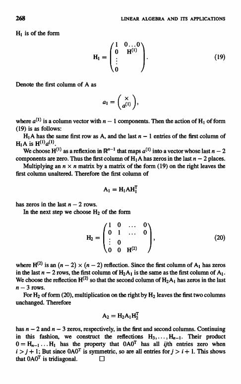
268 LINEAR ALGEBRA AND ITS APPLICATIONS
H, is of the form
1 0...0I
t o HHI
=
0
Denote the first column of A as
xa, =
a column vector with n - 1 components. Then the action of Hl of form(19) is as follows:
H,A has the same first row as A, and the last n - 1 entries of the first column ofH1A is H(I)a(i)
We choose H(') as a reflexion in R"-I that maps al1i into a vector whose last n - 2components are zero. Thus the first column of H, A has zeros in the last n - 2 places.
Multiplying an n x n matrix by a matrix of the form (19) on the right leaves thefirst column unaltered. Therefore the first column of
AI = H1AHj
has zeros in the last n - 2 rows.In the next step we choose H2 of the form
1 0
to 1
H2 =0
a 0 H(2)
(20)
where H(2) is an (n - 2) x (n - 2) reflection. Since the first column of AI has zerosin the last n - 2 rows, the first column of H2A1 is the same as the first column of AI .We choose the reflection H(2) so that the second column of H2A1 has zeros in the lastn - 3 rows.
For H2 of form (20), multiplication on the right by H2 leaves the first two columnsunchanged. Therefore
A2 = H2AIHi
has n - 2 and n - 3 zeros, respectively, in the first and second columns. Continuingin this fashion, we construct the reflections H3,-..,H,,-I. Their product0 = HI has the property that OAOT has all ijth entries zero wheni > j + 1; But since OAOT is symmetric, so are all entries for j > i + 1. This showsthat OAOT is tridiagonal. 0
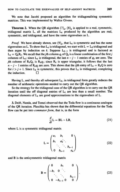
HOW TO CALCULATE THE EIGENVALUES OF SELF-ADJOINT MATRICES 269
We note that Jacobi proposed an algorithm for tridiagonaliring symmetricmatrices. This was implemented by Wallce Givens.
Theorem 2. When the QR algorithm (7)k' (8)k is applied to a real, symmetric,tridiagonal matrix L, all the matrices Lk produced by the algorithm are real,symmetric, and tridiagonal, and have the same eigenvalues as L.
Proof. We have already shown, see (9)k, that Lk is symmetric and has the sameeigenvalues as L. To show that Lk is tridiagonal, we start with L = L0 tridiagonal andthen argue by induction on k. Suppose Lk_, is tridiagonal and is factored asLk = QkRk. We recall that thejth column qj of Qk is a linear combination of the first jcolumns of Lk; since Lk is tridiagonal, the last n - j - 1 entries of qk are zero. Thejth column of RkQk is Rkqj; since Rk is upper triangular, it follows that the lastn - j - I entries of Rkgq are zero. This shows that the ijth entry of Lk = RkQ is zerofor i > j + 1. Since Lk is symmetric, this proves that Lk is tridiagonal, completingthe induction.
Having L, and thereby all subsequent Lk, in tridiagonal form greatly reduces thenumber of arithmetic operations needed to carry out the QR algorithm.
So the strategy for the tridiagonal case of the QR algorithm is to carry out the QRiteration until the off diagonal entries of Lk are less than a small number. Thediagonal elements of Lk are good approximations to the eigenvalues of L.
3. Deift, Nanda, and Tomei observed that the Toda flow is a continuous analogueof the QR iteration. Flaschka has shown that the differential equations for the Todaflow can be put into commutor form, that is, in the form
dL=BL - LB,
where L is a symmetric tridiagonal matrix
(21)
a, b, 0
L= bi a'(22)
0 b,1-i a
and B is the antisymmetric tridiagonal matrix
0 b, 0
-b, 0B=bn 1
0 -b,,_, 0 0
(23)
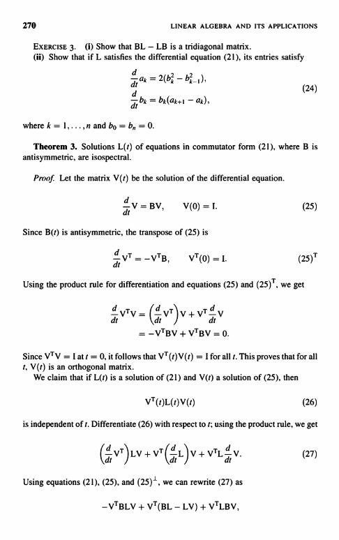
270 LINEAR ALGEBRA AND ITS APPLICATIONS
EXERCISE 3. (i) Show that BL - LB is a tridiagonal matrix.(ii) Show that if L satisfies the differential equation (21), its entries satisfy
ddt ak
= 2(bk - bk-1
d(24)
dtbk = bk(ak+I - ak),
where k = 1,...,n and bo = b = 0.
Theorem 3. Solutions L(t) of equations in commutator form (21), where B isantisymmetric, are isospectral.
Proof. Let the matrix V(t) be the solution of the differential equation.
dV = BV, V(0) = I.t
Since B(t) is antisymmetric, the transpose of (25) is
(25)
dt VT-VTB, VT(O) = I. (25)T
Using the product rule for differentiation and equations (25) and (25)T, we get
dt VTV =(VT)V+VTV
__VTBV+VTBV=0.
Since VTV = I at t = 0, it follows that VT(I)V(t) = I for all I. This proves that for allt, V(t) is an orthogonal matrix.
We claim that if L(t) is a solution of (21) and V(t) a solution of (25), then
VT(t)L(t)V(t) (26)
is independent of t. Differentiate (26) with respect to t; using the product rule, we get
(VT)LV+VT(L)V+VTLV. (27)
Using equations (21), (25), and (25)l, we can rewrite (27) as
-VTBLV + VT(BL - LV) + VTLBV,
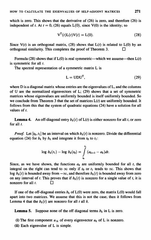
HOW TO CALCULATE THE EIGENVALUES OF SELF-ADJOINT MATRICES 271
which is zero. This shows that the derivative of (26) is zero, and therefore (26) isindependent of t. At t = 0, (26) equals L(O), since V(0) is the identity; so
VT(t)L(t)V(t) = L(0). (28)
Since V(t) is an orthogonal matrix, (28) shows that L(t) is related to L(0) by anorthogonal similarity. This completes the proof of Theorem 3.
Formula (28) shows that if L(0) is real symmetric-which we assume-then L(t)is symmetric for all t.
The spectral representation of a symmetric matrix L is
L = UDUT, (29)
where D is a diagonal matrix whose entries are the eigenvalues of L, and the columnsof U are the normalized eigenvectors of L; (29) shows that a set of symmetricmatrices whose eigenvalues are uniformly bounded is itself uniformly bounded. Sowe conclude from Theorem 3 that the set of matrices L(t) are uniformly bounded. Itfollows from this that the system of quadratic equations (24) have a solution for allvalues of t.
Lemma 4. An off-diagonal entry bk(t) of L(t) is either nonzero for all t, or zerofor all t.
Proof. Let [to, ti] be an interval on which bk(t) is nonzero. Divide the differentialequation (24) for bk by bk and integrate it from to to ti:
h
log bk(ti) - log bk(to) = f (ak+I - ak)dt.to
Since, as we have shown, the functions ak are uniformly bounded for all t, theintegral on the right can tend to oc only if to or tj tends to oc. This shows thatlog bk(t) is bounded away from -oo, and therefore bk(t) is bounded away from zeroon any interval of t. This proves that if bk(t) is nonzero for a single value of t, it isnonzero for all t.
If one of the off-diagonal entries bk of L(0) were zero, the matrix L(0) would fallapart into two matrices. We assume that this is not the case; then it follows fromLemma 4 that the bk(t) are nonzero for all t all k.
Lemma 5. Suppose none of the off diagonal terms bk in L is zero.
(i) The first component uik of every eigenvector uk of L is nonzero.
(ii) Each eigenvalue of L is simple.
272 LINEAR ALGEBRA AND ITS APPLICATIONS
Proof. (i) The first component of the eigenvalue equation
Luk = dkuk
is
alulk +blu2k = dkulk.
(30)
(31)
If ulk were zero, it would follow from (31), since b, # 0, that u2.k = 0. We can thenuse the second component of (30) to deduce similarly that u3,k = 0; continuing inthis fashion, we deduce that all components of uk are zero, a contradiction.
(ii) Suppose on the contrary that dk is a multiple eigenvalue; then its eigenspacehas dimension greater than I. In a space of dimension greater than one, we canalways find a vector whose first component is zero; but this contradicts part (i) ofLemma 5. 0
Lemma 6. The eigenvalues d1,...,d and the first components u1,k,
k = 1, ... , n, of the normalized eigenvectors of L uniquely determine all entriesa1i...,a and b1,...,bk_I of L.
Proof. From the spectral representation (29), we can express the entry L I I = alof L as follows:
al = > dkuik. (32),
From equation (31) we get
blu2k = (dk - al)ulk (33),
Squaring both sides and summing with respect to k gives
bi = E (dk - a1)2uik; (34)l
here we have used the fact that the matrix U is orthogonal, and therefore
2u2k = 1.
We have shown in Lemma 4 that bk(t) doesn't change sign; therefore bk isdetermined by (34) 1. We now set this determination of b1 into (33), to obtain thevalues of u2k.
Next we use the spectral representation (29) again to express a2 = L22 as
a2 = > dku7J. (32)2

HOW TO CALCULATE THE EIGENVALUES OF SELF-ADJOINT MATRICES 273
We proceed as before to the second equation in 30, which we write as
b2u3k = -blulk + (dk - a2)u2k (33)2
Squaring and summing over k gives
b2 = E (-bluk + (dk - a2)u2k)2, (34)2
and so on.Jungen Moser has determined the asymptotic behavior of L(t) as t tends
to00.
Theorem 7. (Moser). L(t) is a solution of equation (21). Denote the eigenvaluesof L by dl , ... , d,,, arranged in decreasing order, and denote by D the diagonal matrixwith diagonal entries dl, ... , d,,. Then
lim L(t) = D.r-.x
Similarly,
(34)
lim L(t) = D_, (34)-3C
where D_ is the diagonal matrix whose diagonal entries are dl.
Proof. We start with the following lemma.
Lemma 8. Denote by u(t) the row vector consisting of the first components ofthe normalized eigenvectors of L(t):
u=(ull,...,ule)-
Claim:
u(t) =u(0)eor
II u(0)eor II
(35)
(36)
Proof. We have shown that when L(t) satisfies (21), L(t) and L(0) are related by(28). Multiplying this relation by V(t) on the left gives
L(t)V(t) = V(t)L(0). (28)'
274 LINEAR ALGEBRA AND ITS APPLICATIONS
Denote as before the normalized eigenvectors of L(t) by Uk(t). Let (28)' act on uk(0).Since
L(0)uk(0) = dkuk(0),
we get
L(t)V(t)uk(0) = dkV(t)uk(0).
This shows that V(t)uk(0) = uk(t) are the normalized eigenvectors of L(t).V(t) satisfies the differential equation (25), AV = By. Therefore uk(t) _
V(t)uk(0) satisfies
dd
Ilk = Buk.
Since B is of form (23), the first component of (37) is
dd Ulk = blu2k
We now use equation (33)I to rewrite the right-hand side:
ddrink = (dk - al)ulk
Define f (t) by
Equation (37)" can be rewritten as
from which we deduce that
where Ck is a constant. So
f (t) =J
, a, (s)ds.0
d (')-d"dt ulk(t) = 0,
ef(')-dx-rUlk = Ck,
(37)
(37)'
Ulk(t) = Cked"F(t),

HOW TO CALCULATE THE EIGENVALUES OF SELF-ADJOINT MATRICES 275
where F(t) = exp [f(t)]. Since f (0) = 0, F(O) = 1, and ck = ulk(0); we obtain
Ulk(t) = ulk(0)ed'`F(t). (38)
In vector notation, (38) becomes
u(t) = u(0)e' F(t).
Since u(t) is the first row of an orthogonal matrix, it has norm 1. This shows that F(t)is the normalizing factor, and it proves formula (36). 0
(i) Since the eigenvalues of L(t) are distinct (see Lemma 5), formula (36) showsthat as t - oo, the first component u 11 (t) of u(t) is exponentially larger than the othercomponents. Since the vector u(t) has norm 1, it follows that as t -' oo, ul 1(t) tendsto 1, and ulk(t), k > 1, tend to zero at an exponential rate.
(ii) Next we take equation (32)1:
al (t) = dkulk(t)
From what we have shown about Ulk(t), it follows that al (t) tends to d1 at anexponential rate as t -' oo.
(iii) To estimate b1 we take the representation (34)1:
bl (t) (dk -a, (t) )2uk (t)
From al (t) -* dl and the fact that u(t) is a unit vector, we deduce that b1 (t) tends tozero at an exponential rate as t - oo.
(iv) The first two rows of u are orthogonal:
ulk(t)u2k(t) = 0.
According to (i), u!l(t) -* 1 and ulk(t) -> 0 exponentially astherefore from (39) that u21 (t) -> 0 exponentially as t -+ oo.
(v) From (31) we deduce that
u2k dk - alulkU22 d2 - al u12
By the explicit formula (38) we can write this as
u2k(t) - dk - al (t) u2k(0)
U22 (t) d2 - a l (t) u22 (0)e
(39)

276 LINEAR ALGEBRA AND ITS APPLICATIONS
Take k > 2; then the right-hand side of (41) tends to zero as t -> oc, and thereforeU2k(t) -> 0 as t -> oo for k > 2. We have shown in (iv) that U21 (t) -> 0 as t -> cc.Since (u21, ... , u2,) is a unit vector, it follows that u22(t) -> 1 exponentially.
(vi) According to formula (32)2,
a2(t) _ dku2k(t).
Since we have shown in (v) that u2k(t) -> 0 for k # 2 and that u22 -> 1, it followsthat a2(t) -> d2.
(vii) Formula (34), represents b2(t) as a sum. We have shown above that allterms of this sum tend to zero as t --> oo. It follows that b2(t) -> 0 ast -> oo, at the usual exponential rate.
The limiting behavior of the rest of the entries can be argued similarly; Deift et al.supply all the details.
Identical arguments show that L(t) tends to D_ as t -> -oo.Moser's proof of Theorem 7 runs along different lines.We conclude this chapter with four observations.Note 1. It may surprise the reader that in Lemma 8 we present an explicit solution.
The explanation is that the Toda lattice, of which (21) is a form, is completelyintegrable. According to Liouville's Theorem, such systems have explicit solutions.
Note 2. Moser's Theorem is a continuous analogue of the convergence of the QRalgorithm to D when applied to a tridiagonal matrix.
Note 3. Deift et al. point out that (21) is only one of a whole class of flows oftridiagonal symmetric matrices that tend to D as t --> oc. These flows are incommutator form (21), where the matrix B is taken as
B = P(L), - p(L)-,
where p is a polynomial, M+ denotes the upper triangular part of M, and M_ denotesits lower triangular part. The choice (23) for B corresponds to the choice p(L) = L.
Note 4. Deift et al. point out that solving numerically the matrix differentialequation (21) until such time when b1,. .. , b become less than a preassigned smallnumber is a valid numerical method for finding approximately the eigenvalues of L.In Section 4 of their paper they present numerical examples comparing the speed ofthis method with the speed of the QR algorithm.
BIBLIOGRAPHY
Deift, P., Nanda, T., and Tomei, C. Ordinary differential equations and the symmetriceigenvalue problem, SIAM J. Numer. Anal. 20 (1983), 1-22.
Flaschka, H. The Joda lattice, I, Phys. Rev. B 9 (1974), 1924-1925.

HOW TO CALCULATE THE EIGENVALUES OF SELF-ADJOINT MATRICES 277
Francis, J. The QR transformation, a unitary analogue of the LR transformation, I, Comput. J. 4(1961), 265-271.
Golub, G. H., and Van Loan, C. F. Matrix Computations, Johns Hopkins University Press,Baltimore, 1989.
Lax, P. D. Integrals of nonlinear equations of evolution and solitary waves, CPAM 21 (1968),467-490.
Moser, J. Finitely many mass points on the line under the influence of an exponentialpotential-an integrable system. In Dynamical Systems, Theory and Applications,Springer-Verlag, New York, 1975, pp. 467-497.
Parlett, B. N. The Symmetric Eigenvalue Problem, Prentice Hall, Englewood Cliffs, NJ, 1980.
Trefathen, L. N., and Bau, D. Numerical Linear Algebra, SIAM, Philadelphia, PA, 1997.
Solutions of Selected Exercises
CHAPTER1
Ex 1. Suppose z is another zero:
x+z=x for all x.
Setx=0:0+z= 0. But also z + 0 = z, so z = 0.
Ex 3. Every polynomial p of degree < n can be written as
p = a,xn-I + a2xn-2 + ... a
Then p - (a, , ... , a,,) is an isomorphism.
Ex 7. If x, , x2 belong to X and to Y,, then x, + x2 belongs to X and Y.
Ex 10. If x; were 0, then
l.xi + 0.x1 = 0.
i0i
Ex 13. (iii) If x, - x2 is in Y, and x2 - x3 is in Y, then so is their sumx, -x2+x2-x3=x, -x3.
Ex 14. Suppose {x,} and {x2} have a vector x3 in common. Then x3 - x, andx3 - x2; but then x, - X2, so {x,} = {x2}.
Linear Algebra and Its Applications, Second Edition, by Peter D. LaxCopyright 6) 2007 John Wiley & Sons, Inc.
278
SOLUTIONS OF SELECTED EXERCISES 279
Ex 16. (i) Polynomials of degree < n that are zero at ti,... , tt can be written in theform
q(t)JJ(t-t;),
where q is a polynomial of degree < n - j. These clearly form a linear space, whosedimension is n -j.
By Theorem 6,
dimX/Y=dimX - dimY=n-(n-j) =j.
The quotient space X/Y can be identified with the space of vector
(p(ti),...,p(tj))
Ex 19. Use Theorem 6 and Exercise 18.
Ex 20. (b) and (d) are subspaces
Ex 21. The statement is false; here is an example to the contrary:
X = R2 = (x,y)spaceU={y=0},v={x=0},w={x=y}.U+v+w=R2,unv={0},Unw={0}vnw={o},unvnw=o.
So
201+1+1-0-0-0-0.
CHAPTER 2
Ex 4. We choose MI = m3; then (9) is satisfied for p(t) = t. For p(t) = I andp(t) = t', (9) says that
2 = 2mi + m2, 3 = 2mia2.
So
1 2nil = 3a2 , and m2 = 2 3a2 ,
from which (ii) follows. (iii) (9) holds for all odd polynomials like t3 and t5. Forp(t) = t4, (9) says that
5=2mia4=2a2,
which holds for a = 3/5.

280 LINEAR ALGEBRA AND ITS APPLICATIONS
Ex 5. Take in1 = m4, m2 = m3, in order to satisfy (9) for all odd polynomials. Forp(t) = I and p(t) = t2 we get two equations easily solved.
Ex 6. (a) Suppose there is a linear relation
all (p) + b12(p) + c13(p) = 0,
Set p = p(x) = (x - 2)(x - g3). Then p(i;2) = p(t;3) = O,p(1) # 0; so we getfrom the above relation that a = 0. Similarly b = 0, c = 0.
(b) Since dim P2 = 3, also dim P, = 3. Since 11, 12, 13 are linearly independent,they span P.
(c 2) Set
P1 (x) = (x - 2)(x - 3)/(I - 2)(I - 3),
and define p2, p3 analogously. Clearly
1;(Pi)=1 if i = j0if i¢j.
Ex 7. e(x) has to be zero for x = (1, 0, -1, 2) and x = (2,3, 1, 1). These yield twoequations for c1, . . . , c4:
C1 -C3+2c4=0, 2c1+3C2+C3+C4=0.
We express c1 and c2 in terms of c3 and c4. From the first equation, c l = C3 - 2c4.Setting this into the second equation gives c2 = -C3 + C4.
CHAPTER 3
Ex 1. If Ty1 = u1, Ty2 = u2, then T(y1 +y2) = u1 + u2, and conversely.
Ex 2. Suppose we drop the ith equation; if the remaining equations do notdetermine x uniquely, there is an x that is mapped into a vector whose componentsexcept the ith are zero. If this were true for all i = 1, . . . , in, the range of the mappingx -3 u would be in-dimensional; but according to Theorem 2, the dimension of therange is < n < in. Therefore one of the equations may be dropped without usinguniqueness; by induction in - n of the equations may be omitted.
Ex 4. Rotation maps the parallelogram 0, x, y, x + y into another parallelogram0, X', y', z'; therefore z' = x' + y'.
ST maps (1, 0, 0) into (0, 1, 0); TS maps (1, 0, 0) into (0, 0, 1).

SOLUTIONS OF SELECTED EXERCISES 281
Ex5. SetTx=u;then (T-'T)x=T-'u=x, and(TT-')u=Tx=u.
Ex 6. Part (ii) is true for all mappings, linear or nonlinear. Part (iii) was illustratedby Eisenstein as follows: the inverse of putting on your shirt and then your jacket istaking off your jacket and then your shirt.
Ex 7. ((ST)1,x) _ (1, (ST)'x);
also((STI,x) = (TI,S'x) = (I,T'S'x),
from which (ST)' = T'S' follows.
Ex 8. (TI, x) = (1, T'x) = (T"I, x) for all x; therefore TI = T"I.
Ex 10. If M = SKS-', then S-'MS = K, and by Theorem 4,
S-'M-'S = K-'.
Ex 11. AB = ABAA-' = A(BA)A-1, by repeated use of the associative law.
Ex 13. The even part of an even function is the function itself.
CHAPTER 4
Ex 1. (DA)s _ DikAkJ = diAjj, (AD)U = AikDki = AjjdJ.
Ex 2. In most texts the proof is obscure.
Ex 4. Choose B so that its range is the nullspace of A, but the range of A is not thenullspace of B.
CHAPTER 5
Ex 1. P(PIoP2(x)) = a(PioP2)P(x). Since Pi0P2(x) = PI(P2(x)),
P(Pi°P2(x)) = P(Pi(P2(x))) = a(Pi)P(P2(x));
also
P(P2(x)) = a(P2)P(x).
Combining these identities yields a(P, P2) = a(Pi)a(P2).

282 LINEAR ALGEBRA AND ITS APPLICATIONS
Ex 2. (c) The signature of the transposition of two adjacent variables xk and xk+iis -1. The transposition of any two variables can be obtained by composingan odd number of interchanges of adjacent variables. The result follows fromExercise 1.
(d) To factor p = as a product p = tk ... ti of transpositions, set
t
1 2...pi...nl
pi 2...I...n
_ 1 2...p2...nt2
I p2...2...n
and so on.
Ex 3. Follows from (7)b.
Ex 4. (iii) When ai = el,... , a,, = e,,, the only nonzero term on the right side in(16) is p = identity.
(iv) When a; and aj are interchanged, the right side of (16) can be written as
where t is the transposition of i and j. The result follows from a(top)a(t)a(p) = -a(p)-
Ex 5. Suppose two columns of A are equal. Then, by (iv),
D(a, a) _ -D(a, a),
so 2D(a, a) = 0.
CHAPTER 6
Ex 2. (a) All terms in (14)' tend to zero.(b) Each component of A N h is a sum of exponential functions of N, with distinct
positive exponents.
Ex 5. (25) is a special case of (26), with q(a) = aN. The general case follows bycombining relations (25) for various values of N.
Ex 7. For x in N,t
(A - aI)'Ax = A(A - dI)dx = 0.
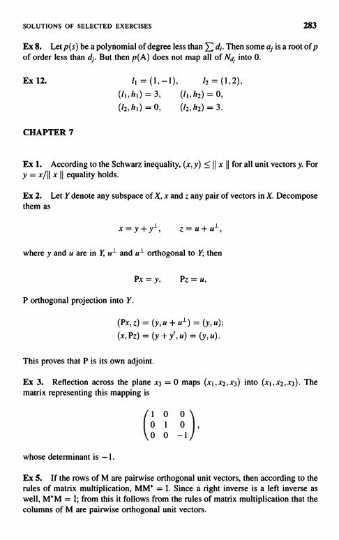
SOLUTIONS OF SELECTED EXERCISES 283
Ex 8. Letp(s) be a polynomial of degree less than > d;. Then some as is a root of pof order less than df. But then p(A) does not map all of Nd; into 0.
Ex 12.
CHAPTER 7
11 = (1,-1), 12 = (1,2),
(li,hi) = 3, (1,,h2) = 0,
(12,hi) = 0, (12,h2) = 3.
Ex 1. According to the Schwarz inequality, (x, y) 5 II x II for all unit vectors y. ForY = x/II x II equality holds.
Ex 2. Let Y denote any subspace of X, x and Zany pair of vectors in X. Decomposethem as
x=Y+y1, Z=U+U1,
where y and u are in Y, u1 and u1 orthogonal to Y; then
Px=y, Pz=u,
P orthogonal projection into Y.
(Px, z) = (y, u + u1) _ (Y, u);
(x, Pz) = (Y + 3'', u) _ (Y, U)
This proves that P is its own adjoint.
Ex 3. Reflection across the plane X3 = 0 maps (x1,x2ix3) into (x,,x2ix3). Thematrix representing this mapping is
1 0 00 1 00 0 -1
whose determinant is -1.
Ex S. If the rows of M are pairwise orthogonal unit vectors, then according to therules of matrix multiplication, MM* = I. Since a right inverse is a left inverse aswell, M*M = I; from this it follows from the rules of matrix multiplication that thecolumns of M are pairwise orthogonal unit vectors.
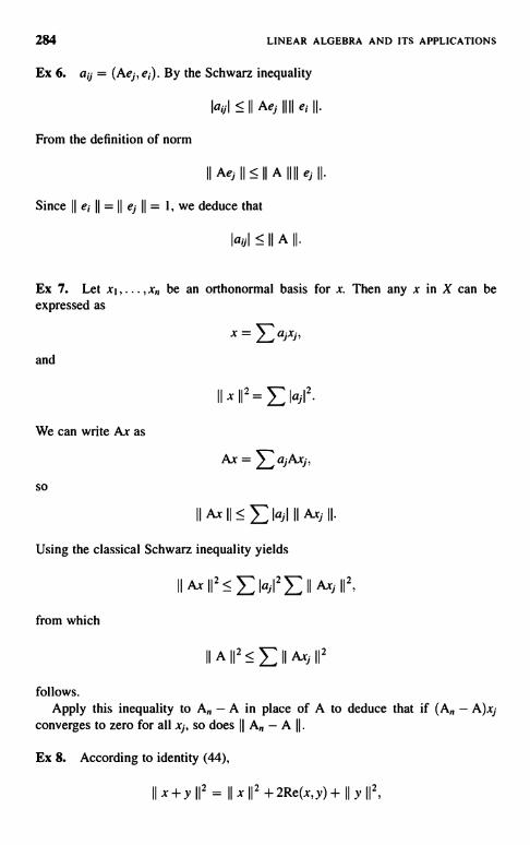
284 LINEAR ALGEBRA AND ITS APPLICATIONS
Ex 6. a,, = (Ae,, e,). By the Schwarz inequality
lain<_11Aee1111er11
From the definition of norm
1IAei1I<11A1111eeII
Since II e; II = II e, II = 1, we deduce that
Ia,,IcIIAII.
Ex 7. Let xl , ... , x be an orthonormal basis for x. Then any x in X can beexpressed as
and
We can write Ax as
Ax= >a,Ax,,
so
11Ax 11<EIajI 11Axi11
Using the classical Schwarz inequality yields
11 Ax 112<1: IajI11:
11 Axi 112.
from which
I1A112<EIIAxj112
follows.Apply this inequality to A - A in place of A to deduce that if (A - A)x,
converges to zero for all x,, so does II A - A II
Ex 8. According to identity (44),
11
x+Y 112 = 11x112+2Re(x.y)+IIY112,
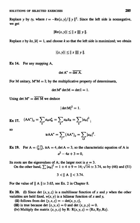
SOLUTIONS OF SELECTED EXERCISES 285
Replace y by ty, where t = -Re(x, y)/ II y 112. Since the left side is nonnegative,we get
IRe(x,y)I <- II x IIII y II.
Replace x by kx, Ikl = 1, and choose k so that the left side is maximized; we obtain
I(x,y)I:IIx1111 yII.
Ex 14. For any mapping A,
det A* = det A.
For M unitary, M*M = I; by the multiplicative property of determinants,
detM* detM = det I = 1.
Using det M* = det M we deduce
IdetMI2=1.
Ex 17.
so
(AA* )ii = 1: alkaki = 1: aikaik = E Iaik l2 .
k k k
trAA* _ E (AA*)ii = E Iaik12.i i,k
Ex 19. For A = (u 3), trA = 4, det A = 3, so the characteristic equation of A is
a2-4a+3 = 0,
Its roots are the eigenvalues of A; the larger root is a = 3.On the other hand, E laik I2 = 1 + 4 + 9 = 14; 14 3.74, so by (46) and (51)
3<IIA II<3.74.
For the value of II A II = 3.65, see Ex. 2 in Chapter 8.
Ex 20. (1) Since det (x, y, z) is a multilinear function of x and y when the othervariables are held fixed, w(x, y) is a bilinear function of x and y,
(ii) follows from det (y, x, z) = - det(x, y, z),(iii) is true because det (x, y, x) = 0 and det (x, y, y) = 0.(iv) Multiply the matrix (x, y, z) by R: R(x, y, z) = (Rx, Ry, Rz).

286 LINEAR ALGEBRA AND ITS APPLICATIONS
By the multiplicative property of determinants, and since det R = 1,
det(x, y, z) = det(Rx, Ry, Rz);
therefore
(w(x, Y), z) = (w(Rx, RY), Rz) =(R*w(Rx,
RY, z)),
from which
w(x, y) = R*w(Rx, Ry)
follows. Multiply both sides by R.(v) Take xo = a(1, 0, 0)', yt, = b(cos O, sin 0,0)'.
fa b cos B zI
(xo x yo, z) = det 0 b sin O Z2
0 0 Z3
_ (ab sin 0)z3
Therefore
x0 x yo = ab sin 0(0, 0, 1)'.
Since a=1Ixo 1I,b=11 Yo II,
11xoxyoII IIxolIIIYo11sin0.
Any pair of vectors x, y that make an angle 0 can be rotated into xo, yo; using (iv)we deduce
11xxY11=11x1111)'II Isin91.
CHAPTER 8
Ex 1. (x, Mx) = M* (x, x) = (x, M"x);
Re(x, Mx) =2
(x, Mx) +2
(x, Mx) = x, M
2M x .
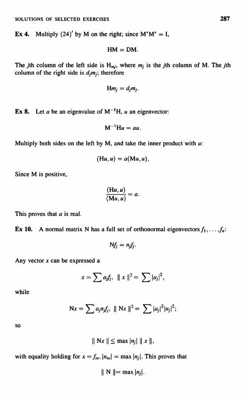
SOLUTIONS OF SELECTED EXERCISES 287
Ex 4. Multiply (24)' by M on the right; since M"M" = I,
HM = DM.
The jth column of the left side is H,,,j, where mj is the jth column of M. The jthcolumn of the right side is djmj; therefore
Hmj = dim`.
Ex 8. Let a be an eigenvalue of M-1H, u an eigenvector:
M-'Hu = au.
Multiply both sides on the left by M, and take the inner product with u:
(Hu, u) = a(Mu, u),
Since M is positive,
(Hu, u)= G.
(Mu, U)
This proves that a is real.
Ex 10. A normal matrix N has a full set of orthonormal eigenvectors fi , ... , f,,:
Nf=nn.
Any vector x can be expressed a
xa,f IIx112= Iajl2while
Nx ajn II Nx 112 =E
IaiI2In l2;
so
II Nxll<maxlnil IIxII,
with equality holding for x = f,,,, In,,,l = max Init. This proves that
IINII=maxlnjl.
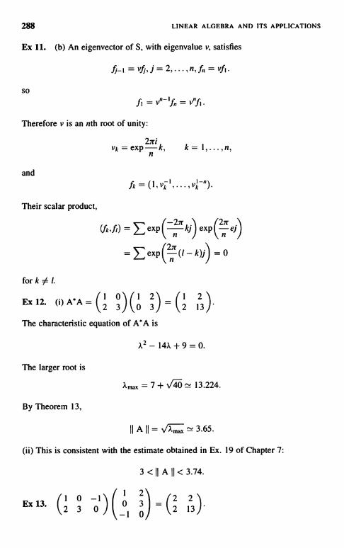
288 LINEAR ALGEBRA AND ITS APPLICATIONS
Ex 11. (b) An eigenvector of S, with eigenvalue v, satisfies
f-i = vf,j= 2,...,n, f, = vfl.
so
f, = v'- Iffn = v".fi
Therefore v is an nth root of unity:
and
Their scalar product,
27riv,. = exp-k, k= 1, .... n,n
fvk', ..,v.-").
(j-, fr) exp2II,r
kj eXp2nn ej
_ exp1 1 =0n
fork54 1.
/Ex12. (i)A`A=(2
3)(0
(1 23
The characteristic equation of A"A is
The larger root is
By Theorem 13,
A2- 14), +9=0.
Amax = 7 + 40 13.224.
11A11= ~3.65.
(ii) This is consistent with the estimate obtained in Ex. 19 of Chapter 7:
3<1A11<3.74.
_ 1 2
Ex 13. (2 3 01) 0 3 )=(2 13)-1 0 /

SOLUTIONS OF SELECTED EXERCISES
The characteristic polynomial of the matrix on the right is
XZ - 15,1 + 22 = 0,
whose larger root is
15 + 137Amax = 2 13.35
By Theorem 13,
1 0 1
3( - v/X--.. -_2 3 0
CHAPTER 9
Ex 2. Differentiate A-' A =I using the product rule:
(A-')A + A' d-A = 0.
Solve for AA-'; (3) results.
Ex 3. Denote (0/
as C; C2 = I, so C" = C for n odd, = I for n even.
So
Ex 6.
By formula (10)
so
expC=C(1 ++ I +I(I=Ce-e_1+1e/+e-1
2 2- (1.54 1.17
1.17 1.54
For Y(t) = exp At,
.
.65.
dY(t) = (expAt)A, Y-'
dY= A.
dt dt
dt log det exp At = tr A,
log det exp At = t tr A.
289

290 LINEAR ALGEBRA AND ITS APPLICATIONS
Thus
detexpAt = exp(t tr A).
Ex 7. According to Theorem 4 in Chapter 6, for any polynomial p, theeigenvalues of p(A) are of the form p(a), a an eigenvalue of A. To extend thisfrom polynomials to the exponential function we note that ee is defined as thelimit of polynomials, em(s) that are defined by formula (12). To complete theproof we apply Theorem 6.
In Ex. 6 we have shown that det exp A = exp(tr A); this indicates that themultiplicity of e° as an eigenvalue of eA is the same as the multiplicity of a as aneigenvalue of A.
CHAPTER 10
Ex 1. In formula (6) for f we may take aj to be either the positive or negativesquare root. This shows that if H has n distinct, nonzero eigenvalues, H has 2° squareroots. If one of the nonzero eigenvalues of H has multiplicity greater then one, H hasinfinitely many square roots.
Ex 3. A = (2 5) is positive; it maps (1, 0) into (1, 2). B = C 2 5) is positive; it maps(1, 0) into (1, -2). The vectors (1, 2) and (1, -2) make an angle > n/2, so AB + BAis not positive. Indeed,
AB+BA= 6 00 42
has one negative eigenvalue.
Ex 4. (a) Apply Theorem 5 twice.(b) Apply Theorem 5 k times,
where 2k = m.(c) The limit
m[M'/m - I] < m[NI /m - I]
gives
log M < log N.
SOLUTIONS OF SELECTED EXERCISES 291
Note. (b) remains true for all positive exponents m > 1.
Ex 5. Choose A and B as in Exercise 3, that is positive matrices whosesymmetrized product is not positive. Set
M=A, N=A+tB,
t a sufficiently small positive number. Clearly, M < N.
N2 = A2 + t(AB + BA) + t2B2;
for t small the term t2 B is negligible compared with the linear term. Therefore for tsmall N22 is not greater than M2.
Ex 6. We claim that the functions f(s) = -(s+t)-I, t positive, are monotonematrix functions. For if 0 < M < N, then 0 < M + tI < N + tI, and so byTheorem 2,
(M+tI)-1 > (N+tI)-'.
The function f (s) defined by (19) is the limit of linear combinations with positivecoefficents of functions of the form s and - (s + t) -I, t > 0. The linear combinationsof monotone matrix functions is monotone, and so are their limits.
Note 1. Loewner also proved the converse of the theorem stated: Every monotonematrix function is of form (19).
Note 2. Every function f(s) of form (19) can be extended to an analytic functioninto the complex upper half plane Im s > 0, so that the imaginary part off (s) ispositive there, and zero on the positive real axis s > 0. According to a theorem ofHerglotz, all such functions f (.s) can be represented in the form (19).
It is easy to verify that the functions s, 0 < in < 1, and the function log s havepositive imaginary parts in the upper half plane.
Ex 7. The matrix
Gij= ,r,>0,r;+rj+lis a Gram matrix:
Gij = J f (t)f (t)dt, fj(t) = tri-'0
Ex 10. By the Schwarz inequality, and the definition of the norm of M - N,
(u, (M - N)u) < II u II II (M - N)u II
<IIu11211M-NII=dIIu1I?

292
Therefore
LINEAR ALGEBRA AND ITS APPLICATIONS
(u, Mu) < (u, Nu) + d 11 u 112 = (u, (N + dI)u).
This proves that M < N + dl; the other inequality follows by inter changing the roleof M and N.
Ex 11. Arrange the m; in increasing order:
Suppose the n; are not in increasing order, that is that for a pair of indices i < j,n; > nj. We claim that interchanging n; and n1 increases the sum (51):
n;mi + njmj < nlmi + n,mj.
For rewrite this inequality as
(ni-nj)mi+(nz-ni)mj=(n;-n1)(mi-mi)<0,
which is manifestly true. A finite number of interchanges shows that (51) ismaximized when the n; and m, are arranged in the same order.
Ex 12. If Z were not invertible, it would have zero as an eigenvalue, contradictingTheorem 20.
Let h be any vector; denote Z- I by k. Then
(Z-'h, h) = (k,Zk);
Since the self-adjoint part of Z is positive, the right side above is positive. But thenso is the left side, which proves that the self-adjoint part of Z- 1 is positive.
Ex 13. When A is invertible, AA* and ASA are similar:
A*A = A-IAA*A,
and therefore have the same eigenvalues. Noninvertible A can be obtained as the
limit of a sequence of invertible matrices.
Ex 14. Let u be an eigenvector of A*A, with nonzero eigenvalue:
A*Au=ru, r#0.

SOLUTIONS OF SELECTED EXERCISES 293
Denote Au as v; the vector v is nonzero, for if Au = 0, it follows from the aboverelation that u = 0.
Let A act on the above relation:
AA*Au = rAu
which can be rewritten as
AA*v = rv;
which shows that v is an eigenvector of AA`, with eigenvalue r.A maps the eigenspace of A*A with eigenvalue r into the eigenspace of AA*; this
mapping is 1-to-1. Similarly A* maps the eigenspace of AA* into the eigenspace ofA*A in a 1-to-I fashion. This proves that these eigenspaces have the samedimension.
Ex 15. Take Z = (o 2), a some real number; its eigenvalues are 1 and 2. But
Z+Z* =
is not positive when a > \/8-.
CHAPTER 11
Ex 1. If M, = AM, Mf = M*A* = -MA.
Then
(M*M), = M' M + M*M, = -M*AM + M*AM = 0.
Since M*M = I at t = 0, M*M = I for all t. At t = 0, detM = I, therefore detM = 1 for all t. This proves that M(t) is a rotation.
Ex 5. The nonzero eigenvalues of a real antisymmetric matrix A are pure imaginaryand come in conjugate pairs ik and -ik. The eigenvalues of A2 are 0, -k22, -k22, sotr A2 = -2k2. The diagonal entries of A'- are -(a2 + b2), -(a2 + c2) and-(b2 + c22), so tr A22 = -2(a2 + b2 + c22). Therefore k = a2 + b'- + c2.
Ex 6. The eigenvalues of eA! are ea`, where a are the eigenvalues of A. Since theeigenvalues of A are 0, ±ik, the eigenvalues of eAt are 1 and et4'. From Af = 0 wededuce that eA'f =f; thus f is the axis of the rotation eA,. The trace of eA, is
294 LINEAR ALGEBRA AND ITS APPLICATIONS
I + e'4" + e-'R' = 2 cos kt + 1. According to formula (4)', the angle of rotation 9 ofM = eA, satisfies 2 cos 0 + I = tr eA,. This shows that 0 = kt = a'- + b2 + c21.
0 a b 0 d eEx8. A= -a 0 c , B= -d 0 g ;
(-b -c 0 -e -g 0
their null vectors are
-c -gfA = b J, fB = e
-a -d(ad + be bg -ag
AB = - ce ad + cg ae
-cd bd be + cg
Therefore tr AB = -2(ad + be + cg), whereas the scalar product of fA and In iscg + be + ad.
Ex 9. BA can be calculated like AB, given above. Subtracting we get
0 ec - bg -dc + agAB-BA= bg-ec 0 db - ae
do - ag ae - db 0
Therefore
ae - dbf A,B] = ag - do
bg - ec
We can verify that fA x fB = f A,B] by using the formula for the cross product inChapter 7.
CHAPTER 12
Ex 2. (a) Let {K, } be a collection of convex sets, denote their intersection by K. If xand y belong to K, they belong to every K;. Since K; is convex, it contains the linesegment with endpoints x and y. Since this line segment belongs to all K;, it belongsto K. This shows that K is convex.
(b) Let x and y be two points in H + K; that means that they are of the form
x=u+z, y=v+w, uandvinH, zandwinK.
SOLUTIONS OF SELECTED EXERCISES 295
Since H is convex, au + (I - a)v belongs to H, and since K is convexa Z + (1 - a) w belongs to H for 0 < a < 1. But then their sum
au+(1-a)v+az+(1-a)w=a(u+z)+(1 -a)(v+w)=ax+(1-a)y
belongs to H + K. This proves that H + K is convex.
Ex 6. Denote (u, v) as x. If both u and v are < 0, then x/r belongs to K for anypositive r, no matter how small. So p(x) = 0.
If 0 < v and u < v, then x/r = (r , E) belongs to K for r > v, but no smaller r.Therefore p(x) = v. We can argue similarly in the remaining case.
Ex 7. If p(x) < 1, p(y) < 1, and 0 < a < 1, then by sub-additivity andhomogeneity of p,
P(ax + (1 - a)y) < P(ax) + P((1 - a)y) = ap(x) + (1 - a)P(y) < 1.
This shows that the set of x : p(x) < 1 is convex.To show that the set p(x) < 1 is open we argue as follows. By subadditivity and
positive homogeneity
P(x + h) s P(x) + P(ty) = P(x) + rp(y).
Since p(x) < 1, p(x) + tp(y) < 1 for all t positive but small enough.
Ex 8.
qs(m + 1) = sup(m + 1)(x)xinS
= sup(in(x) + 1(x)) < sup m(x) + sup 1(x) = qs(m) + qs(l).xinS xinS xinS
Note. This is a special case of the result that the supremum of linear functions issubadditive.
Ex 10.
q(1) = sup I(X)
xinSUT
= max{sup t(x) sup F(x)} = max{gs(1),gT(1)}.xinS xinT
Ex 16. Suppose all pj are positive. Define
k k
)'k Pjxj/ > pj.

296
Then
LINEAR ALGEBRA AND ITS APPLICATIONS
k
Pj
)'k+I = k+lyk + -4-- xk+I
We claim that all points yk belong to the convex set containing x;, ... , x,,,. Thisfollows inductively, since yi = xi, and yk+I lie on the line segment whose endpointsare yk and xk+l. Finally,
m
y...=EPix/i
Ex 19. Denote by Pi, P2i P3 the following 3 x 3 permutation matrices
1 0 0 0 1 0 0 0 1
Pi = 0 1 0, P2 = 0 0 1, P3 = 1 0 0.0 0 1 1 0 0 0 1 0
Then
Similarly define
I I I 11 1 1\
3P1 +3P2+3P3=3 1 1 1) M.1 1 I
1 0 0 0 1 0 0 0 1
P4= 0 0 1 P5= 1 0 0 P6= 0 1 00 1 0 0 0 1 1 0 0
Then
3P4+3P5+IP6=M.
Ex 20. A set S in Euclidean space is open if for every point x in S there is a ball11 y - x 11 < e centered at x that belongs to S. Suppose S is convex and open; thatmeans that there exist positive numbers e; such that x + tei belongs to S for Itl < e;;here e; denotes the unit vectors. Denote min e; by e; it follows that the pointsx ± fee, i = 1, ... , n belong to S. Since S is convex, the convex hull of these pointsbelongs to S; this convex hull contains a ball of radius e/f centered at x.
The converse is obvious.
SOLUTIONS OF SELECTED EXERCISES 297
CHAPTER 13
Ex 3. We claim that the sign of equality holds in (21). For if not, S would belarger than s, contrary to (20); this shows that the supremum in (16) is amaximum.
Replacing Y, y, and j by - Y, -y, -j turns the sup problem into inf, and vice versa.This shows that the In f in (18) is a minimum.
CHAPTER 14
Ex 2. x - z = (x - y) + (y - z); apply the subadditive rule (1)ij.
Ex 5. From the definition of the Ixl,, and Ixlx norms we see that
Ixlx < lxlp < nlxl'..
Take the pth root:
Ixl«. 5 lxl, 5 n'lvlxl>.
Since n1/n tends to I asp tends to oc, lxl = lim lxl1, follows.p-.x
Ex 6. Introduce a basis and represent the points by arrays of real numbers. Since allnorms are equivalent, it suffices to prove completeness in the lxlx norm.
Let {x } be a convergent sequence in the Ixl,,, norm. Denote the components of x,,by x,,,j. It follows from lx - xml1,I. -> 0 that
lxnj - Xnrjl - 0
for every j. Since the real numbers are complete, it follows that
lim X" j = xj.?I- X
Denote by x the vector with components xJ; it follows that
lim lx,, - xl, = 0.
For another proof see Theorem 3.

298 LINEAR ALGEBRA AND ITS APPLICATIONS
CHAPTER 15
Ex 1. According to (i), ITxi < clxl. Apply this to IT(xn - x)l < clx,, - xI.
Ex 3. We have shown above that
(I-R)T"=I-R"+I
Multiply both sides on the left by S-1:
T" = S-I - S-IRn+I
Therefore
IT"-S-1I < IS-IRn+II < IS-'IIR"+II.
Since IRI < 1, IR' 1I < IRI"+' tends to zero as n -> 00,
Ex 5. Decompose n modulo in:
n=kin+r, 0<r<m.
Then
Rn = Rkm+r = (R"' )kRt
therefore
JR"'IklR`I
as n tends to oo, so does k; therefore if IR'l < 1, IR"I tends to zero as n tends to oo.That is all that was used in the proof in Ex. 3, that T" tends in norm to S-I.
Ex 6. The components of y = Tx are
Y; _ tixi.
Since Ixil 5 Ixlx,
IYiI Itiillxlx
So b'Ix < max Ei I1ijiIXIx; (23) follows
SOLUTIONS OF SELECTED EXERCISES 299
CHAPTER 16
Ex 1. What has to be shown is that if Px < ax, then A _> A(P). To see this considerPT, the transpose of P; it, too, has positive entries, so by Theorem 1 it has a dominanteigenvalue A(PT) and a corresponding nonnegative eigenvector k:
PTk = X(PT)k.
Take the scalar product of Px < Ax with k; since k is a nonnegative vector
(Px, k) < A(x, k)
The left side equals (x, PTk) = JX(PT) (x, k). Since x and k are nonnegative vectors,(x, k) is positive, and we conclude that X (PT) < X. But P and pT have the sameeigenvalues, and therefore the largest eigenvalue A(P) of P equals the largesteigenvalue A(PT) of PT,
Ex 2. Denote by p. the dominant eigenvalue of P", and by k the associatedeigenvector:
P"'k = pk.
Let P act on this relation:
P"k = PPk = pPk,
which shows that Pk, too, is an eigenvector of P" with eigenvalue it. Since thedominant eigenvalue has multiplicity one, Pk = ck. Repeated application of P showsthat Pk = c"k. Therefore c' = A. From Pk = ck we deduce that c is real andpositive; therefore it is the real root All"'. Since the entries of k are positive,c = 1z 11' is the dominant eigenvalue of P.
Bibliography
Axler, Sheldon. Linear Algebra Done Right, Undergraduate Texts in Mathematics, Springer-Verlag, New York, 1996.
Bellman, Richard. Introduction to Matrix Analysis, McGraw-Hill, New York, 1960.
Courant, Richard, and Hilbert, David. Methods of Mathematical Physics. Vol. I, WileyInterscience, New York, 1953.
Edwards, Harold M. Linear Algebra, Birkhauser, Boston, 1995.
Golub, Gene, and Van Loan, Charles. Matrix Computations, 2nd ed., The John HopkinsUniversity Press, Baltimore, 1989.
Greub, Werner. Linear Algebra, 4th ed., Graduate Texts in Mathematics, Springer-Verlag,New York, 1975.
Halmos, Paul R. Finite Dimensional Vector Spaces, Undergraduate Texts in Mathematics,Springer-Verlag, New York, 1974.
Halmos, Paul R. Linear Algebra Problem Book, Dolciani Mathematical Expositions #16,Mathematical Association of America, Providence, RI, 1995.
Hoffman, Kenneth, and Kunze, Ray. Linear Algebra, Prentice Hall, Englewood Cliffs, NJ,1971.
Hom, R. A., and Johnson, C. R. Matrix Analysis, Cambridge University Press, 1985.Hom, R. A., and Johnson, C. R. Topics in Matrix Analysis, Cambridge University Press,
1991.
Lancaster, P., and Tismenetsky, M. The Theory of Matrices, Academic Press, New York,1985.
Lang, Serge. Linear Algebra, 3rd ed., Undergraduate Texts in Mathematics, Springer-Verlag,New York, 1987.
Lay, David C. Linear Algebra and Its Applications, Addision-Wesley, Reading, MA, 1994.Roman, Steven. Advanced Linear Algebra, Graduate Texts in Mathematics, Springer-Verlag,
New York, 1992.
Linear Algebra and Its Applications. Second Edition, by Peter D. LaxCopyright i; 2007 John Wiley & Sons, Inc.
300
BIBLIOGRAPHY 301
Serre, Denis. Matrices: Theory and Applications, Graduate Texts in Mathematics, Springer-Verlag, New York, 2002.
Strang, Gilbert. Linear Algebra and Its Applications, 3rd ed., Harcourt, Brace, Jovanovich,San Diego, 1988.
Trefethenr, Lloyd N., and Bay, David. Numerical Linear algebra, SLAM, 1997.
Valenza, Robert J. Linear Algebra, An Introduction to Abstract Mathematics, UndergraduateTexts in Mathematics, Springer-Verlag, New York, 1993.

APPENDIX 1
Special Determinants
There are some classes of matrices whose determinants can be expressed by compactalgebraic formulas. We give some interesting examples.
Definition. A Vandermonde matrix is a square matrix whose columns form ageometric progression. That is, let at, ... , a be n scalars; then V(ai, ... , a,,) is thematrix
1 1
a1 aV(ai,...,a.) _
al-t
(1)
Theorem 1
det V(ai,... , an) = 11 (aj - a1). (2)j>i
Proof. Using formula (16) of Chapter 5 for the determinant, we conclude thatdet V is a polynomial in the a1 of degree less than or equal to n(n - 1)/2. Whenevertwo of the scalars a, and aa, i O j, are equal, V has two equal columns and so itsdeterminant is zero; therefore, according to the factor theorem of algebra, det V isdivisible by aj - a1. It follows that det V is divisible by the product
fl(aj - a1).j>1
Linear Algebra and Its Applications, Second Edition, by Peter D. LaxCopyright Q 2007 John Wiley & Sons, Inc.
302

APPENDIX l: SPECIAL DETERMINANTS 303
This product has degree n(n - 1)/2, the same as the degree of det V. Therefore
det V = c JJ(aj - ai), (2)'j>i
c,, a constant. We claim that c = 1; to see this we use the Laplace expansion (26)of Chapter 5 for det V with respect to the last column, that is, j = n. We get in thisway an expansion of det V in powers of a,,; the coefficient of a;,-' isdet V (a i , ... , I ). On the other hand, the coefficient of an-1 on the right of (2)'is (aj - ai). Using expression (2)' for V(aj.... we deduce thatc = 1. An explicit calculation shows that C2 = 1; hence by induction c,, = 1 forall n, and (2) follows.
Definition. Let a, , ... , an and b1,... , b be 2n scalars. The Cauchy matrixC(al.... ,a,,;b1,...,b,,) is the n x n matrix whose ijth element is 1/(ai +aj):
C(a, b) =
Theorem 2.
detC(a,b) _fj>i (aj - ai)(bj - bi)
fij(ai+bj) (3)
Proof. Using formula (16) of Chapter 5 for the determinant of C(a, b), and usingthe common denominator for all terms we can write
det C(a, b) =P(a' b)
rji.j (ai + bj) '(4)
where P(a, b) is a polynomial whose degree is less than or equal to n2 - n.Whenever two of the scalars ai and aj are equal, the ith and jth row of C(a, b) areequal; likewise, when bi = bj, the ith and jth column of C(a, b) are equal. In eithercase, det C(a, b) = 0; therefore, by the factor theorem of algebra, the polynomialP(a, b) is divisible by (aj - a,) and by (bj - b,), and therefore by the product
fi(aj - ai)(bj - bi).pi
The degree of this product is n2 - n, the same as the degree of P; therefore,
P(a, b) = c JJ(aj - ai)(bj - b;), (4)'j>i

304 APPENDIX I: SPECIAL DETERMINANTS
c,, a constant. We claim that c = 1; to see this we use the Laplace expansion forC(a, b) with respect to the last column, j = n; the term corresponding to the element1/(an + bn) is
detC(al,...)an-l;bl,...,b,,_,) Ian+bn.
Now set an = bn = d; we get from (4) and (4)' that
C(aii...,d;b1,...,d)
cn ! In>i (d - al) (d - b,) lln>j>f (aj - ai)(bj - bi)2d fl,>,(d +a,)(d+b,) rjij<n(a, +bj)
From the Laplace expansion we get
C(a1i...,d;b1,...,d)
= ZdC(al,... , an-1; b 1 , . . . , On- 1) + other terms.
Multiply both expressions by 2d and set d = 0; using (4)' to expressC(a1 i ... , an-,; b1, ... , b,,), we deduce that cn = cn_1. An explicit calculationshows that Cl = 1, so we conclude by induction that cn = 1 for all n; (3) now followsfrom (4) and (4)'.
Note: Every minor of a Cauchy matrix is a Cauchy matrix.
EXERCISE I. Let
P(S) = Xl + x2s + + xnsn-1
be a polynomial of degree less than n. Let al,. .. , an be n distinct numbers, and letpl,... ,p,, be n arbitrary complex numbers; we wish to choose the coefficientsx1i... , xn so that
p(ai) =pi, i = 1,...,n.
This is a system of n linear equations for the n coefficients x1. Find the matrix of thissystem of equations, and show that its determinant is # 0.
EXERCISE 2. Find an algebraic formula for the determinant of the matrix whoseijth element is
1
1+aiaj;
here al, . . . , an are arbitrary scalars.

APPENDIX 2
The Pfaffian
Let A be an n x it antisymmetric matrix:
AT = -A.
We have seen in Chapter 5 that a matrix and its transpose have the same determinant.We have also seen that the determinant of -A is (-1)" detA so
detA = det AT = det(-A) = (-1)" det A.
When n is odd, it follows that det A = 0; what can we say about the even case?Suppose the entries of A are real; then the eigenvalues come in complex
conjugate pairs. On the other hand, according to the spectral theory of anti-self-adjoint matrices, the eigenvalues of A are purely imaginary. It follows that theeigenvalues of A are (-ill, ... , i).1, ... , iA,,12). Their product is (HA1)2, apositive number; since the determinant of a matrix is the product of its eigenvalues,we conclude that the determinant of an antisymmetric matrix of even order with realentries is nonnegative.
Far more is true:
Theorem of Cayley. The determinant of an antisymmetric matrix A ofeven order is the square of a homogeneous polynomial of degree n/2 in the
entries of A:
det A = P2.
P is called the Pfaffian.
Linear Algebra and Its Applications. Second Edition, by Peter D. LaxCopyright 2007 John Wiley & Sons, Inc.
305
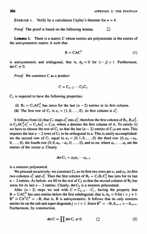
306 APPENDIX 2: THE PFAFFIAN
EXERCISE I. Verify by a calculation Cayley's theorem for n = 4.
Proof. The proof is based on the following lemma. O
Lemma 1. There is a matrix C whose entries are polynomials in the entries ofthe antisymmetric matrix A such that
B = CACT (1)
is antisymmetric and tridiagonal, that is, bf = 0 for li - jl > 1. Furthermore,detC54 0.
Proof. We construct C as a product
C, is required to have the following properties:
(i) B, = C,ACi has zeros for the last (n - 2) entries in its first column.(ii) The first row of C, is e, = (1,0,... , 0), its first column is ei .
It follows from (ii) that C, maps ei into ei ; therefore the first column of BI, BIei ,is CIACT of = C,Aef = C,a, where a denotes the first column of A. To satisfy (i)we have to choose the rest of C, so that the last (n - 2) entries of C,a are zero. Thisrequires the last n - 2 rows of C, to be orthogonal to a. This is easily accomplished:set the second row of CI equal to e2 = (0, 1, 0, ... , 0) the third row (0, a3, -a2,0, ... , 0), the fourth row (0, 0, a4, -a3, 0, ... , 0), and so on, where a1,. .. , a,, are theentries of the vector a. Clearly
detCI
is a nonzero polynomial.We proceed recursively; we construct C2 so its first two rows are e, and e2, its first
two columns e and e2. Then the first column of B2 = C2BIC2 has zero for its lastn - 2 entires. As before, we fill in the rest of C2 so that the second column of B2 haszeros for its last n - 3 entries. Clearly, detC2 is a nonzero polynomial.
After (n - 2) steps we end with C = C , ,_ 2 . . . C1, having the property thatB = CACT has zero entries below the first subdiagonal, that is, by = 0 for i > j + 1.BT = CATCT = -B, that is, B is antisymmetric. It follows that its only nonzeroentries lie on the sub and super diagonals j = i + 1. Since BT = -B, b;,;_ I = -b;.;+, .Furthermore, by construction,
detC=fldetC;#0. 13 (2)
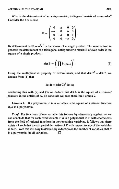
APPENDIX 2: THE PFAFFIAN 307
What is the determinant of an antisymmetric, tridiagonal matrix of even order?Consider the 4 x 4 case
B=
0 a 0 0-a 0 b 0
0 -b 0 c
0 0 -c 0
Its determinant det B = a2c2 is the square of a single product. The same is true ingeneral: the determinant of a tridiagonal antisymmetric matrix B of even order is thesquare of a single product,
detB = (flb2k.z_I)2. (3)
Using the multiplicative property of determinants, and that det CT = det C, wededuce from (1) that
det B = (det C)2 det A;
combining this with (2) and (3) we deduce that det A is the square of a rationalfunction in the entries of A. To conclude we need therefore Lemma 2.
Lemma 2. If a polynomial P in n variables is the square of a rational functionR, R is a polynomial.
Proof For functions of one variable this follows by elementary algebra; so wecan conclude that for each fixed variable x, R is a polynomial in x, with coefficientsfrom the field of rational functions in the remaining variables. It follows that thereexists a k such that the kth partial derivative of R with respect to any of the variablesis zero. From this it is easy to deduce, by induction on the number of variables, that Ris a polynomial in all variables.

APPENDIX 3
Symplectic Matrices
In Chapter 7 we studied orthogonal matrices 0; they preserve a scalar product:
(Ox, Oy) = (x, y).
Scalar products are symmetric bilinear functions; in this appendix we investigatelinear maps that preserve a nonsingular bilinear alternating function of the form(x, Ay), A a real anti-self-adjoint matrix, det A # 0. It follows that A must be of evenorder 2n. It suffices to specialize to A = J, where, in block notation,
(1)
I is the n x n unit matrix.
EXERCISE I. Prove that any real 2n x 2n anti-self-adjoint matrix A, detA # 0,can be written in the form
A = FJFT,
J defined by (1), F some real matrix, det F 0 0.
The matrix J has the following properties, which will be used repeatedly:
J2 = -I, J-t = -J = JT.
Theorem 1. A matrix S that preserves (x, Jy):
(Sx,JSy) _ (x,Jy)
Linear Algebra and Its Applications, Second Edition, by Peter D. LaxCopyright Cc'j 2007 John Wiley & Sons, Inc.
(2)
(3)
308
APPENDIX 3: SYMPLECTIC MATRICES 309
for all x and y, satisfies
STJS = J (4)
and conversely.
Proof. (Sx, JSy) = (x, STJSy). If this is equal to (x, Jy) for all x, y, STSJy = J,.for all y.
A real matrix S that satisfies (4) is called a symplectic matrix. The set of allsymplectic matrices is denoted as Sp(n).
Theorem 2. (i) Symplectic matrices form a group under matrix multiplication.(ii) If S is symplectic, so is its transpose ST.
(iii) A symplectic matrix S similar to its inverse S-1.
Proof. (i) It follows from (4) that every symplectic matrix is invertible. Thatthey form a group follows from (3). To verify (ii), take the inverse of (4); using (2)we get
S-IJ(ST)-1 = J.
Multiplying by S on the left, ST on the right shows that ST satisfies (4).To deduce (iii) multiply (4) by S-1 on the right and J-1 on the left. We get that
J-ISTJ = S-1, that is, that S-1 is similar to ST. Since ST is similar to S, (iii)follows.
Theorem 3. Let S(t) be a differentiable function of the real variable 1, whosevalues are symplectic matrices. Define G(t) by
dt S = GS.
Then G is of the form
(5)
G = JL(t), L self-adjoint. (6)
Conversely, if S(t) satisfies (5) and (6) and S(0) is symplectic, then S(t) is a family ofsymplectic matrices.
Proof. For each t (4) is satisfied; differentiate it with respect to t:
(.5r)J5 + STJIS = 0.

310 APPENDIX 3: SYMPLECTIC MATRICES
Multiply by S-1 on the right, (ST)-1 on the left:
(ST) -1 dt ST J + J (dt S) S-1 = 0.
We use (5) to define G:
Taking the transpose we get
Setting these into (7) gives
G= (s)s-'.
GT =(ST)_1 d ST.
dt
GTJ + JG = 0,
from which (6) follows. F1
EXERCISE 2. Prove the converse.
(7)
We turn now to the spectrum of a symplectic matrix S. Since S is real, its complexeigenvalues come in conjugate pairs, that is, if A is an eigenvalue, so is A. Accordingto part (iii) of Theorem 2, S and S-1 are similar; since similar matrices have the samespectrum, it follows that if \ is an eigenvalue of S, so is A-' and it has the samemultiplicity. Thus the eigenvalues of a symplectic matrix S come in groups of four:
with three exceptions:
(a) When A lies on the unit circle, that is, CAI = 1, then A-1 = X, so we onlyhave a group of two.
(b) When A is real, . = A, so we only have a group of two.(c) A = I or -1.
The possibility is still open that A = ±1 are simple eigenvalues of S; but thiscannot occur according to
Theorem 4. For a symplectic matrix S, A = 1 or -1 cannot be a simpleeigenvalue.
Proof. We argue indirectly: suppose, say, that A = -1 is a simple eigenvalue,with eigenvector h:
Sh = -h. (8)

APPENDIX 3: SYMPLECTIC MATRICES
Multiplying both sides by STJ and using (4) we get
Jh = -STJh,
311
(8)'
which shows that Jh is eigenvector of ST with eigenvalue -1.We choose any self-adjoint, positive matrix L, and set G = JL. We define the one-
parameter family of matrices S(t) as e'"S; it satisfies
dtS(t) = GS(t), S(0) = S. (9)
According to Theorem 3, S(t) is symplectic for all t.If S(0) has -1 as eigenvalue of multiplicity one, then for t small, S(t) has a single
eigenvalue near -1. This eigenvalue A equals -1, for otherwise A-I would beanother eigenvalue near -1. According to Theorem 8 of Chapter 9, the eigenvectorh(t) is a differentiable function of t. Differentiating Sh = -h yields
(.Ls)h + Sh, = -h,, h, = dt h.
Using (9) and (8) we get
Gh=h,+Sh,.
Form the scalar product with Jh; using (8)' we get
(Gh, Jh) = (h,, Jh) + (Sh,, Jh) = (h,, Jh) + (h,, ST Jh)(10)
= (h,,Jh) - (h,,Jh) = 0.
According to (6), G = JL; set this into (10); since by (2), jTj = 1, we have
(JLh, Jh) = (Lh, JTJh) = (Lh, h) = 0. (10)'
Since L was chosen to be self-adjoint and positive, h = 0, a contradiction.
EXERCISE 3. Prove that plus or minus I cannot be an eigenvalue of oddmultiplicity of a symplectic matrix.
Taking the determinant of (4), using the multiplicative property, and thatdet ST = det S we deduce that (det S)2 = I so that det S = 1 or - 1. More istrue.

312 APPENDIX 3: SYMPLECTIC MATRICES
Theorem S. The determinant of a symplectic matrix S is 1.
Proof. Since we already know that (det S)2 = 1, we only have to exclude thepossibility that det S is negative. The determinant of a matrix is the product of itseigenvalues. The complex eigenvalues come in conjugate pairs; their product ispositive. The real eigenvalues 0 1, - l come in pairs A, A', and their product ispositive. According to Exercise 3, -1 is an eigenvalue of even multiplicity; so theproduct of the eigenvalues is positive. 0
We remark that it can be shown that the space Sp(n) of symplectic matrices isconnected. Since (det S)2 = I and since S = I has determinant 1, it follows thatdet S = I for all S in Sp(n).
Symplectic matrices first appeared in Hamiltonian mechanics, governed byequations of the form
dtu = JHu,
where u(t) lies in l 2n, H is some smooth function in R2i, and H. is its gradient.
Definition. A nonlinear mapping u -> v is called a canonical transformation ifits Jacobian matrix 9v/au is symplectic.
Theorem 6. A canonical transformation changes every Hamiltonian equation(11) into another equation of Hamiltonian form:
dtv = JK,
where K(v(u)) = H(u).
EXERCISE 4. Verify Theorem 6.

APPENDIX 4
Tensor Product
For an analyst, a good way to think of the tensor product of two linear spaces is totake one space as the space of polynomials in x of degree less than n, the other asthe polynomials in y of degree less than m. Their tensor product is the space ofpolynomials in x and y, of degree less than n in x, less than in in y. A natural basis forpolynomials are the powers 1 , x, . . . , x"- t and 1, y, ... , y"'- 1, respectively; a naturalbasis for polynomials in x and y is xi);i, i < n, j < M.
This sets the stage for defining the tensor product of two linear spaces U and Vasfollows: Let lei} be a basis of the linear space U, {fj} a basis for the linear space V.Then lei Of j} is a basis for their tensor product U ® V.
It follows from this definition that
dim U ®V = (dim U)(dim V). (1)
The definition, however, is ugly, since it uses basis vectors.
EXERCISE I. Establish a natural isomorphism between tensor products definedwith respect to two pairs of distinct bases.
Happily, we can define U ® V in an invariant manner.Take the collection of all formal sums
E ui ®vi, (2)
where ui and vi are arbitrary vectors in U and V, respectively. Clearly, these sumsform a linear space.
Sums of the form
(ut+u2)®v-u1 ®v-u2®v (3)
Linear Algebra and Its Applications, Second Edition, by Peter D. LaxCopyright `:i 2007 John Wiley & Sons. Inc.
313

314
and
APPENDIX 4: TENSOR PRODUCT
u®(VI +V2) - u®vi - u®v2 (3)'
are special cases of (2). These, and all their linear combinations, are called null sums.Using these concepts we can give a basis-free definition of tensor product.
Definition. The tensor product U ® V of two finite-dimensional linear spaces Uand V is the quotient space of the space of all formal sums (2) modulo all null sums(3), (3)'.
This definition is basis-free, but a little awkward. Happily, there is an elegant wayof presenting it.
Theorem 1. There is a natural isomorphism between U ® V as defined aboveand Y(U', V), the space of all linear mappings of U' into V, where U' is the dual of U.
Proof. Let Eu; ® vi be a representative of an equivalence class in the quotientspace. For any l in If, assign to I the image El(u;)v; in V. Since every null sum ismapped into zero, this mapping depends only on the equivalence class.
The mapping L,
I -+ E l(u;)v
is clearly linear and the assignment
{ u; ®v; } - L (4)
also is linear. It is not hard to show that every L in 2(U', V) is the image of somevector in U ®V. 0
EXERCISE 2. Verify that (4) maps U ® V onto 2'(U', V).
Theorem 1 treats the spaces U and V asymmetrically. The roles of U and V can beinterchanged, leading to an isomorphism of U ® V and 2'(V', U). The dual of a mapL:U'-> V is of course a map L': V1 - U.
When U and V are equipped with real Euclidean structure, there is a natural wayto equip U ® V with Euclidean structure. As before, there are two ways of goingabout it. One is to choose orthonormal bases {e;}, {J} in U and V respectively, anddeclare {ei ®f } to be an orthonormal basis for U ® V. It remains to be shown thatthis Euclidean structure is independent of the choice of the orthonormal bases; this iseasily done, based on the following lemma.
APPENDIX 4: TENSOR PRODUCT 315
Lemma 2. Let u, z be a pair of vectors in U, v, w a pair of vectors in V. Then
(u (9 v,z ®w) = (u,z)(v, w). (5)
Proof. Expand u and z in terms of the ei, v and w in terms of f j.
u = 57 aie1, z = > bkek,
v=1,cjf, w=>2d,f,.
Then
u®v=Eaicje,®f, z ®w = 1: bkd,ek ®fi;
so
(u 0 v, z (& w) _ aicjbidjj
_ (>aibi)(>cJdJ) = {u, z) (v, w). O
Take the example presented at the beginning, where V is the space of polynomialsin x of degree < n, and V is the space of polynomials in y of degree <m. Define in Uthe square integral over an x-interval A as the Euclidean norm, and in V the squareintegral over a y-interval B. Then the Euclidean structure in U 0 V defined by (5) isthe square integral over the rectangle A x B.
We show now how to use the representation of U 0 V as .t(U', V) to derive theEuclidean structure in U ® V from the Euclidean structure of U and V. HereU'= U, soU®Vis&(U,V).
Let M and L belong to £(U, V), and let L* be the adjoint of L. We define
(M,L) = trL*M. (6)
Clearly this depends bilinearly on M and L. In terms of orthonormal bases, M and Lcan be expressed as matrices (mij) and (lij), and L* as the transpose (iji). Then
trL*M = Eljimji-
Setting L = M, we get
IIM112=(M,M)=Em,
consistent with our previous definition.Complex Euclidean structures can be handled the same way.
316 APPENDIX 4: TENSOR PRODUCT
All of the foregoing is pretty dull stuff. To liven it up, here is a one-line proof ofSchur's peculiar theorem from Chapter 10, Theorem 7: if A = (A;j) and B = (B,j)are positive symmetric n x n matrices then so is their entry by entry productM = (AijB7j).
Proof. It was observed in Theorem 6 of Chapter 10 that every positive symmetricmatrix can be written as a Gram matrix:
Alj = (u;, uj), U. C U, linearly independent,
Bij = (vj, vj), v; C V, linearly independent.
Now define g; in U ® V to be u, ® v;; by (5), (g;,gj) = (u;, uj)(v;, vj) = A;jB;j.This shows that M is a Gram matrix, therefore nonnegative.
EXERCISE 3. Show that if {u;} and {vj} are linearly independent, so are u; ® v;.Show that My is positive.
EXERCISE 4. Let u be a twice differentiable function of xl, ... , x defined in aneighborhood of a point p, where u has a local minimum. Let (A;j) be a symmetric,nonnegative matrix. Show that
uAij (p) ? 0.
8x; axj
APPENDIX 5
Lattices
Definition. A lattice is a subset L of a linear space X over the reals with thefollowing properties:
(i) L is closed under addition and subtraction; that is, if x and y belong to L, sodo x + y and x - y.
(ii) L is discrete, in the sense that any bounded (as measured in any norm) set ofX contains only a finite number of points of L.
An example of a lattice in l t is the collection of points x = withinteger components xi. The basic theorem of the subject says that this example istypical.
Theorem 1. Every lattice has an integer basis, that is, a collection of vectors inL such that every vector in the lattice can be expressed uniquely as a linearcombination of basis vectors with integer coefficients.
Proof. The dimension of a lattice L is the dimension of the linear space it spans.Let L be k-dimensional, and let p, .... , Pk be a basis in L for the span of L; that is,every vector tin L can be expressed uniquely as
t = E aapi, a1 real. (1)
Consider now the subset of those vectors t in L which are of form (1) with a1 between0 and 1:
0 < a1 < 1, j = 1,...,k. (2)
Linear Algebra and Its Applications. Second Edition, by Peter D. LaxCopyright 2007 John Wiley & Sons, Inc.
317
318 APPENDIX 5: LATTICES
This set is not empty, for its contains all vectors with aj = 0 or 1. Since L is discrete,there are only a finite number of vectors t in L of this form; denote by q, that vector tof form (1), (2) for which a, is positive and as small as possible.
EXERCISE I. Show that a, is a rational number.
Now replace p, by q, in the basis; every vector tin L can be expressed uniquely as
k
t = b,q, + b1p1, bf real.2
(3)
We claim that b, occurring in (3) is an integer; for if not, we can subtract a suitableinteger multiple of q, from t so that the coefficient b, of q, lies strictly between0 and 1:
0<b, < 1.
If then we substitute into (3) the representation ( 1 ) of q, in terms of p, , ... , Pk andadd or subtract suitable integer multiples of P2, ... , pk, we find that the p,coefficient oft is positive and less than the p, coefficient of q,. This contradicts ourchoice of qi.
We complete our proof by an induction on k, the dimension of the lattice.Denote by La the subset of L consisting of those vectors t in L whose representationof form (3), b, is zero. Clearly 4 is a sublattice of L of dimension k - 1; byinduction hypothesis La has an integer basis q2.... , qk. By (3), q, ... , qk is aninteger basis of L.
An integer basis is far from unique as is shown in the following theorem.
Theorem 2. Let L be an n-dimensional lattice in R". Let q, .... , qn andr,, ... , rn be two integer bases of L; denote by Q and R the matrices whose columnsare q, and r;, respectively. Then
Q = MR,
where M is a unimodular matrix, that is, a matrix with integer entries whosedeterminant is plus or minus 1.
EXERCISE 2. (i) Prove Theorem 2.(ii) Show that unimodular matrices form a group under multiplication.
Definition. Let L be a lattice in a linear space X. The dual of L, denoted as L', isthe subset of the dual X' of X consisting of those vectors t; for which (t, ) is aninteger for all tin L.
APPENDIX 5: LATTICES 319
Theorem 3. (i)The dual of an n-dimensional lattice in an n-dimensional linearspace is an n-dimensional lattice.
(ii) L" = L.
EXERCISE 3. Prove Theorem 3.
EXERCISE 4. Show that L is discrete if and only if there is a positive number dsuch that the ball of radius d centered at the origin contains no other point of L.

APPENDIX 6
Fast Matrix Multiplication
How many scalar multiplication are needed to form the product C of two n x nmatrices A and B? Since each entry of C is the product of a row of A with a columnof B, and since C has n2 entries, we need n3 scalar multiplication, as well as n3 - n2additions. It was a great discovery of Volker Strassen that there is a way ofmultiplying matrices that uses many fewer scalar multiplication and additions. Thecrux of the idea lies in a clever way of multiplying 2 x 2 matrices:
A - (all a12
a21 a22 / ' B= (b21 b22
AB =C= CI1 C12
C21 Cn
c1I = a11b11 +a12b21, c12 =a, ib12 + a12b22, and soon. Define
I = (all + an)(bii + b22),
II = (a21 +a22)bu,
III =au(b12-b22),
IV = an(b21 - b11),
V = (a1I +a12)b22,
VI = (a2I -a,,) (b, I + b12),
VII = (a12 -an)(b2l +b22)
Linear Algebra and Its Applications, Second Edition, by Peter D. LaxCopyright Q 2007 John Wiley & Sons, Inc.
(1)
320

APPENDIX 6: FAST MATRIX MULTIPLICATION 321
A straightforward but tedious calculation shows that the entries of the product matrixC can be expressed as follows:
cll =I+IV-V+VII, c12=III+V,c21 =II+IV, C22 =I+III-II+VI.
(2)
The point is that whereas the standard evaluation of the entries in the product matrixuses two multiplications per entry, therefore a total of eight, the seven quantities in(1) need only seven multiplications. The total number of additions and subtractionsneeded in (1) and (2) is 18.
The formulas (1) and (2) in no way use the commutativity of the quantities a andb. Therefore, (1) and (2) can be used to multiply 4 x 4 matrices by interpreting theentries a,j and b;; as 2 x 2 block entries. Proceeding recursively in this fashion, wecan use (1) and (2) to multiply any two matrices A and B of order 2k.
How many scalar multiplications M(k) have to be carried out in this scheme? Inmultiplying two square matrices of order 2k we have to perform sevenmultiplications of blocks of size 2k- I x 21-'. This takes 7M(k - 1) scalarmultiplications. So
M(k) = 7M(k - 1).
Since M(O) = 1, we deduce that
M(k) = 7k = 2k log2 7 = nl0927(3)
where n = 2k is the order of the matrices to be multiplied.Denote by A(k) the number of scalar additions-subtractions needed to multiply
two matrices of order 2k using Strassen's algorithm. We have to perform 18 additionsand 7 multiplications of blocks of size 21-I x 21-1; the latter takes 7A(k - 1)additions, the former 18(2k-I)2 = 9.22k-I. So altogether
A(k) = 9.22-I + 7A(k - 1).
Introduce B(k) = 7-kA(k); then the above recursion can be rewritten as
B(k) = 2 (4)+B(k- 1).
Summing with respect to k we get, since B(O) = 0,
B(k) 2 C7)l < (2)(3) 6:

322 APPENDIX 6: FAST MATRIX MULTIPLICATION
therefore
A(k) < 6 x 7' = 6 x 2R i°s2 7 = 6nIOs2 7 (4)
Since loge 7 = 2.807 - is less than 3, the number of scalar multiplications requiredin Strassen's algorithm is for n large, very much less than n3 the number of scalarmultiplications required in the standard way of multiplying matrices.
Matrices whose order is not a power of 2 can be turned into one by adjoining asuitable number of 1 s on the diagonal.
Refinements of Strassen's idea have led to further reduction of the number ofscalar multiplications needed to multiply two matrices. It has been conjectured thatfor any positive a there is an algorithm that computes the product of two n x nmatrices using cost n2+E scalar multiplication, where the contant depends on e.

APPENDIX 7
Gershgorin's Theorem
This result can be used to give very simple estimates on the location of theeigenvalues of a matrix, crude or accurate depending on the circumstances.
Gershgorin Circle Theorem. Let A be an n x n matrix with complex entries.Decompose it as
A = D + F, (1)
where D is the diagonal matrix equal to the diagonal of A; F has zero diagonalentries. Denote by d, the ith diagonal entry of D, and by f, the ith row of F. Define thecircular disc C, to consist of all complex numbers z satisfying
Iz-d;I<_Vill, i=1,...,n. (2)
The 1-norm of a vector f is the sum of the absolute values of its components; seeChapter 14. Claim: every eigenvalue of A is contained in one of the discs C,.
Proof. Let u be an eigenvector of A,
Au = Au, (3)
normalized as Jul. = 1, where the oo-norm is the maximum of the absolute value ofthe components u u of u. Clearly, 1 u 1 < 1 for j and it, = 1 for some i. WritingA = D + F in (3), the ith component can be written as di +fiu = A, which can berewritten as
Linear Algebra and Its Applications, Second Edition, by Peter D. LaxCopyright C 2007 John Wiley & Sons, Inc.
323
324 APPENDIX 'J: GERSHGORIN'S THEOREM
The absolute value of the product fu is <V1 1 Jul., so
IA - diI : Vill Jul. = Vill. 0
EXERCISE. Show that if C; is disjoint from all the other Gershgorin discs, then C;contains exactly one eigenvalue of A.
In many iterative methods for finding the eigenvalues of a matrix A, A istransformed by a sequence of similarity transformations into Ak so that Ak tends to adiagonal matrix. Being similar to A, each Ak has the same eigenvalues as A.Gershgorin's theorem can be used to estimate how closely the diagonal elements ofAk approximate the eigenvalues of A.

APPENDIX 8
The Multiplicity of Eigenvalues
The set of n x n real, self-adjoint matrices forms a linear space of dimensionN = n(n + I )/2. We have seen at the end of Chapter 9 that the set of degeneratematrices, that is, ones with multiple eigenvalues, form a surface of codimension 2,that is, of dimension N - 2. This explains the phenomenon of "avoided crossing,"that is, in general, self-adjoint matrices in a one-parameter family have all distincteigenvalues. By the same token a two-parameter family of self-adjoint matricesought to have a good chance of containing a matrix with a multiple eigenvalue. Inthis appendix we state and prove such a theorem about two parameter families of thefollowing form:
aA=bB+cC, a2+b2+c2= 1. (1)
Here A, B, C are real, self-adjoint n x n matrices, and a, b, c are real numbers.
Theorem (Lax). If n = 2(mod 4), then there exist a, b, c such that (1) isdegenerate, that is, has a multiple eigenvalue.
Proof. Denote by )V the set of all nondegenerate matrices. For any N in H denoteby k, < k2 < ... < k the eigenvalues of N arranged in increasing order and by ujthe corresponding normalized eigenvectors:
Nuj=kjuj, 11uj11=1,j=1,...,n. (2)
Note that each uj is determined only up to a factor ±1.Let 0 < t < 27r, be a closed curve in N. If we fix uj(O), then the normalized
eigenvector uj(t) can be determined uniquely as continuous functions of t. Since fora closed curve N(27r) = N(O),
uj(21r) = Tju(O), Tj = ±1. (3)
Linear Algebra and Its Applications. Second Edition, by Peter D. LaxCopyright 2007 John Wiley & Sons, Inc.
325

326 APPENDIX 8: THE MULTIPLICITY OF EIGENVALUES
The quantities -rj, j = 1, . . . , m are functionals of the curve N(t). Clearly:(i) Each Tj is invariant under homotopy, that is, continuous deformation in H.
(ii) For a constant curve, that is, N(t) independent of t, each Tj = 1.
N(t) = cos to + sin tB, 0 < t < 27r
is a closed curve in H. Note that N is periodic, and
N(t + a) = -N(t).
It follows that
and that
Aj(t+7r) = -An-j+1(t)
(4)
uj(t + ir) = Pjun f+1(t), (5)
where pj = ± 1. Since uj is a continuous function of t, so is pj; but since pj can onlytake on discrete values, it is independent of t.
For each value of t, the eigenvectors u 1(t), ... , u (t) form an ordered basis. Sincethey change continuously they retain their orientation. Thus the two ordered bases
u1(0),...,u,,(0) and ul(ir),...,un(ir) (6)
have the same orientation. By (5),
ul (Tr), ... , un(ir) = Pl un(0), ... , (0). (6)'
Reversing the order of a basis for n even is the same as n/2 transpositions. Sinceeach transposition reverses orientation, for n = 2(mod 4) we have an odd number oftranspositions. So in order for (6) and (6)' to have the same orientation,
n
Writing this product as
rjpj1
n/2
[JPjP j+l = -1,
we conclude there is an index k for which
PkPn-kA l = -1. (7)

APPENDIX 8: THE MULTIPLICITY OF EIGENVALUES
Using (5) twice, we conclude that
uk(21r) = Pkun-k+1(1) = PkPn-k+luk(0)
327
This shows, by (3), that Tk = PkPn-k+1, and so by (7) that Tk = -1. This provesthat the curve (4) cannot be deformed continuously in H to a point. But the curve (4)is the equator on the unit sphere a2 + b2 + c2 = 1; if all matrices of form (1)belonged to H, the equator could be contracted on the unit sphere to a point,contradicting Tk = -1
EXERCISE. Show that if n = 2(mod4), there are non x n real matrices A, B, Cnot necessarily self-adjoint, such that all their linear combinations (1) have real anddistinct eigenvalues.
Friedland, Robbin, and Sylvester have extended the theorem to alln f3, 4(mod 8), and have shown that it does not hold when n an 0, ±1(mod 8).
These results are of interest in the theory of hyperbolic partial differentialequations.
BIBLIOGRAPHY
Friedland, S., Robbin, J., and Sylvester, J. On the crossing rule, CPAM 37 (1984), 19-37.Lax, P. D. The multiplicity of eigenvalues, BuIL AMS 6 (1982), 213-214.

APPENDIX 9
The Fast Fourier Transform
In this appendix we study functions defined on a finite number of points arrangedperiodically. A function on these points is a sequence of numbers, generallycomplex, U1 ,. .. , un. In many applications, uk stands for the value at x = k/n of aperiodic function u(x) defined on the unit interval [0, 1]. The vector (ul, ... , un) = uis a discrete approximation of the function u(x).
In this appendix we shall analyze the cyclic shift mapping S defined by
S(ul,...,un) = (u2,u3,...,un,ul)
The mapping S preserves the Euclidean norm
IIu1112=E1uk12;
such mappings are called unitary (see Chapter 8). According to Theorem 9 inChapter 8, unitary mappings have a complete set of pairwise orthogonaleigenvectors ej, with eigenvalues Aj that are complex numbers of absolute value 1.We shall now calculate the eigenvector and eigenvalues of 5.
From the eigenvalue equation Se = ale, we deduce that the components(ul, ... , un) of a satisfy
u2=AuI, u3=)6u2i...,un=XUn-1, u1 =Xun.
We set ul =1l and then deduce from the first n - I equations above that
u2=A2, u3-A3a...,un= A n ,
Linear Algebra and Its Applications, Second Edition, by Peter D. LaxCopyright 0 2007 John Wiley & Sons, Inc.
328

APPENDIX 9: THE FAST FOURIER TRANSFORM 329
and from the last equation that 1 = V. This shows that the eigenvalues A are the nroots of unity Aj = exp 2 ' j), and the corresponding eigenvectors
ej = V). (1)
Each eigenvector ek has norm I I ej I I = vl"n-.Every vector it = (u1, ... , un) can be expressed as a linear combination of
eigenvectors:
u = > ajej.
Using the explicit expression (1) of the eigenvector, we can rewrite (2) as
uk = aj exp(2-'riJk
.
n
(2)
(2)'
Using the orthogonality of the eigenvectors, along with their norm IIejMI = f, wecan express the coefficients aj as
1 " 2iri 1aj = (u, ej)/n = -
( ..uk exp - Jk (3)
n 1
Jn
It is instructive to compare formulas (2)' and (3) to the expansion of periodicfunctions in terms of their Fourier series. But first we have to rewrite equation (2)' asfollows. Suppose n is odd; we rewrite the last (n - 1)/2 terms in the sum (2)' byintroducing a new index of summation I related to j by j = n -1. Then
2,ri 2iri
(-2,riexp(,-jk) = exp -(n -1))k = exp-1k
n n n
Setting this into (2)', we can rewrite it as
(i-1)/2 12ni= aj exp ( -Jk (4)Uk
where we have reverted to denote the index of summation by j and where aj isdefined by (3). A similar formula holds when n is even.
Let u(x) be a periodic function of period 1. Its Fourier series representation is
u(x) = bj exp(27rijx), (5)
330 APPENDIX 9: THE FAST FOURIER TRANSFORM
where the Fourier coefficients are given by the formula
Ib = u x ex 2irJi'x dx.f P(- ) (6)
0
Setting x = k/n into (5) gives
u(n) k(2Jri J.k).-P n
(5)'
The integral (6) can be approximated by a finite sum at the equidistant pointsxA = k/n:
n
n
bl ,,, u - exp Jk/\n/ \ 2n r
(6)'
Suppose u is a smooth periodic function, say d times differentiable. Then the(n - 1)/2 section of the Fourier series (5) is an excellent approximation to u(x):
(n-I)/2u(x) = E bjexp(2irijx) + O(n-d )
-(n- 1)/2(7)
Similarly, the approximating sum on the right-hand side of (6)' differs by 0(n-d)from b". It follows that if in (3) we take u,t = u(L), aj differs from bi by O(n-d).
When u is a smooth periodic function, its derivatives may be calculated bydifferentiating its Fourier series term by term:
o'u(x) _ bb(2rrij)"' exp(2 r(jx).
The truncated series is an excellent approximation to r'u. It follows therefore that
C27riai(2rrij),,, exp -jk
(n-I)/2 n
is an excellent approximation to 'u(k), provided that uA in (3) is taken as u(nTherein lies the utility of the finite Fourier transform: It can be used to obtain highlyaccurate approximations to derivatives of smooth periodic functions, which can thenbe used to construct very accurate approximate solutions of differential equations.
On the other hand, operations such as multiplication of u by a given smoothfunction can be carried out fast and accurately when u is represented by its values atthe points k/n. Since in the course of a calculation the operation of differentiation
APPENDIX 9: THE FAST FOURIER TRANSFORM 331
and multiplication may have to be carried out alternately many times, it is of greatestimportance that the finite Fourier transform, the passage from the point values(u1.... , Uk) to the set of Fourier coefficients (a,,. . . , a,,) and its inverse, be carriedout as fast as possible. The rest of this appendix is devoted to this task.
Using formula (3), n multiplications are needed for the computation of eachFourier coefficient aj provided that the roots of unity exp (- 2d1), . . , n1= 1, ... ,
are precomputed. Since there are n coefficients to compute, we need a total of 712multiplications to carry out the finite Fourier transform.
It is therefore a considerable surprise that the finite Fourier transform can becarried out performing only n log n multiplications, where the log is to base 2. Hereis how it works:
Assume that n is even. Denote the array of coefficients (a1, ... , a,,)' by A and thearray (ut, ... , by U. Then relation (3) can be written in matrix form
1
A =n (8)
where the it x it matrix F is F;, = Wik, where w = exp(- 2 `). The colums of F areso we can write F as
F,, _
Reorder the columns of F by first listing all of even order e2i ... , e and then the oddones, Denote the rearranged matrix by F,,:
r=
Fully written out, Fr, looks like this; here we have used the facts thatW" = 1, cv"/2 = -I:
W2 W4
W4 WR
W2 W4
W4 W1
WW2
-W ... -v 1
-W- ... -(0_1)
3
6W 1(,) 2
This suggests that we represent F, in 2 x 2 block form
= Fr
Bit B12
F" B21 B22) (9)
332 APPENDIX 9: THE FAST FOURIER TRANSFORM
We can immediately identify B11 and B21 as Fn/2. We claim that
B12 = DFn/2, B22 = -DFn/2,
where D is an n/2 x n/2 diagonal matrix with diagonal entries wT o see this, note that the first r o w of B 12 can be written as w 1(w2, w4, ... ., 1)thesecond row as w2(cv4, cvs, ... ,1), and so on. This shows that B12 = DFn/2; sinceB22 = -B 12, the rest follows.
Rearrange the components of the vector A and U, putting first all the even ones,followed by the odd ones:
Ur=
UeUve.
add Ar = (Add ) .
Then, (8) can be rewritten as
AT =1FnUr.n
Break AT and Ur into blocks; by (9):
Aeven _ 1 Fn/2 DFn/2 Uvven
Aodd) - n Fn/2 -DFn/2 Uodd
So
Aeven = n (Fn/2Ueven + DFn/2Uodd),
Aodd =1
n (Fn/2Ueven - DFn/2Uodd).
(10)
Denote by M(n) the number of multiplications needed to calculate the vector A,given U. Using formula (10), see that we have to apply Fn/2 to two different vectorswhich takes 2 M(n/2) multiplications; we have to apply D twice, another nmultiplications, and we have to multiply by 1/n, another n multiplications. Soaltogether
M(n) = 2M(n/2) + 2n. (11)
If n is a power of 2, we have similar relations between M(n/2) and M(n/4), and so on;putting these relations together, we get
M(n) = n loge n, (12)
where loge denotes logarithm to base 2.

APPENDIX 9: THE FAST FOURIER TRANSFORM 333
There are some additional computational expenses; additions and rearrangementsof vectors. The total amount of work is 5n 1092 n flops (floating point operations).
The inverse operation, expressing uk in terms of the aI [see (2)'], is the same,except that w is replaced by ao, and there is no division by n.
There is an interesting discussion of the history of the Fast Fourier Transform inthe 1968 Arden House Workshop.
When Cooley and Tukey's paper on the Fast Fourier Transform appeared,Mathematical Reviews reviewed it by title only; the editors did not grasp itsimportance.
BIBLIOGRAPHY
Cooley, J. W., and Tukey, J. W. An algorithm for the machine calculation of complex FourierSeries, Math. Comp. 19 (1965), 297-301.
The 1968 Arden House Workshop on Fast Fourier Transform, IEEE Trans. Audio Electro-acoust. AU-17, (1969).
Van Loan, C. F. Introduction to Scientific Computing, Prentice Hall, Englewood Cliffs, NJ.

APPENDIX 10
The Spectral Radius
Let X be a finite-dimensional Euclidean space, and let A be a linear mapping of Xinto X. Denote by r(A) the spectral radius of A:
r(A) = max jail, (1)
where ai rangers over all eigenvalues of A. We claim that
lit IIAAIlt/j = r(A), (2)jyx
where IIA'II denotes the norm of the jth power of A.
Proof. A straightforward estimate [see inequality (48)j of Chapter 7] shows that
IIAill t/' >_ r(A).
We shall show that
lim supllA'IIt11 < r(A).
(3)
(4)
Combining (3) and (4) gives (2).We can introduce an orthonormal basis in X, thereby turning X into C", with the
standard Euclidean norm (lxt I2 + ... + Ix512)1/2 , and A into an it x n matrix withcomplex entries. We start with the Schur factorization of A: D
Theorem 1. Every square matrix A with complex entries can be factored as
A = QTQ«,
Linear Algebra and Its Applications. Second Edition, by Peter D. LaxCopyright (t_; 2007 John Wiley & Sons, inc.
(5)
334

APPENDIX 10: THE SPECTRAL RADIUS 335
where Q is unitary and T is upper triangular:
ty =0 fori>j.
(5) is called a Schur factorization of A.
Proof If A is a normal matrix, then according to Theorem 8 of Chapter 8 it has acomplete set of orthogonal eigenvectors qi,... , q,,, with eigenvalues a,, ... , a,,:
Aqk = akgk (6)
Choose the qk to have norm 1, and define the matrix Q as
Q =
Since the columns of Q are pairwise orthogonal unit vectors, Q is unitary. Equations(6) can be expressed in terms of Q as
AQ = QD, (6)'
where D is the diagonal matrix with D,tk = at. Multiplying (6)' by Q* on the rightgives a Schur factorization of A, with T = D.
For arbitrary A we argue inductively on the order n of A.We have shown at the beginning of Chapter 6 that every n x n matrix A has at
least one eigenvalue a, possibly complex:
Aq = aq. (7)
Choose q to have norm 1, and complete it to an orthonormal basis q,, ... , q,,, q, = q,and define the matrix U to have columns q, .... , q,,:
U =
Clearly, U is a unitary matrix, and the first column of AU is aq:
AU = (aq,c...... c,,)
The adjoint U* of U has the form
(7)'
I 9i
=
9U.
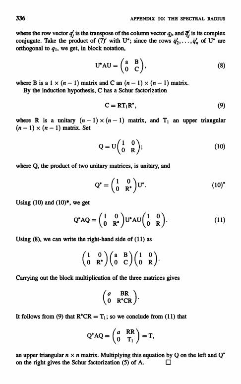
336 APPENDIX 10: THE SPECTRAL RADIUS
where the row vector q; is the transpose of the column vector qj, and 41 is its complexconjugate. Take the product of (7)' with U*; since the rows of U* areorthogonal to qt, we get, in block notation,
U*AU = f a C ), (8)
where B is a 1 x (n - 1) matrix and C an (n - 1) x (n - 1) matrix.By the induction hypothesis, C has a Schur factorization
C = RT1R*, (9)
where R is a unitary (n - 1) x (n - 1) matrix, and T1 an upper triangular(n - 1) x (n - 1) matrix. Set
Q=U` 0 R);
where Q, the product of two unitary matrices, is unitary, and
Q.=(0R*)u*.
(10)
Using (10) and (10)*, we get
Q AQ- (0 R*)U AU( 0 R). (11)
Using (8), we can write the right-hand side of (11) as
1
(0 R*)(0
C) (0 R
Carrying out the block multiplication of the three matrices gives
a BR0 R*CR
It follows from (9) that R*CR = T1; so we conclude from (11) that
* _ a RRQAQ 0 T1
=T,
an upper triangular n x n matrix. Multiplying this equation by Q on the left and Q*on the right gives the Schur factorization (5) of A.
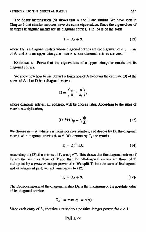
APPENDIX Io: THE SPECTRAL RADIUS 337
The Schur factorization (5) shows that A and T are similar. We have seen inChapter 6 that similar matrices have the same eigenvalues. Since the eigenvalues ofan upper triangular matrix are its diagonal entries, T in (5) is of the form
T=DA+S, (12)
where DA is a diagonal matrix whose diagonal entries are the eigenvalues as, ..., anof A, and S is an upper triangular matrix whose diagonal entries are zero.
EXERCISE I. Prove that the eigenvalues of a upper triangular matrix are itsdiagonal entries.
We show now how to use Schur factorization of A to obtain the estimate (3) of thenorm of N. Let D be a diagonal matrix
di 0D p d ,
whose diagonal entries, all nonzero, will be chosen later. According to the rules ofmatrix multiplication,
(D-'TD)i = tied . (13)
We choose dj = e1, where a is some positive number, and denote by DE the diagonalmatrix with diagonal entries dj = er. We denote by Te the matrix
TE = D:'TDE. (14)
According to (13), the entries of TE are to S. This shows that the diagonal entries ofTE are the same as those of T and that the off-diagonal entries are those of T,multiplied by a positive integer power of e. We split TE into the sum of its diagonaland off-diagonal part; we get, analogous to (12),
Te = DA + Se. (12)e
The Euclidean norm of the diagonal matrix DA is the maximum of the absolute valueof its diagonal entries:
IIDAI I = max IajI = r(A).
Since each entry of SE contains a raised to a positive integer power, for e < 1,
IISEI I < cc,
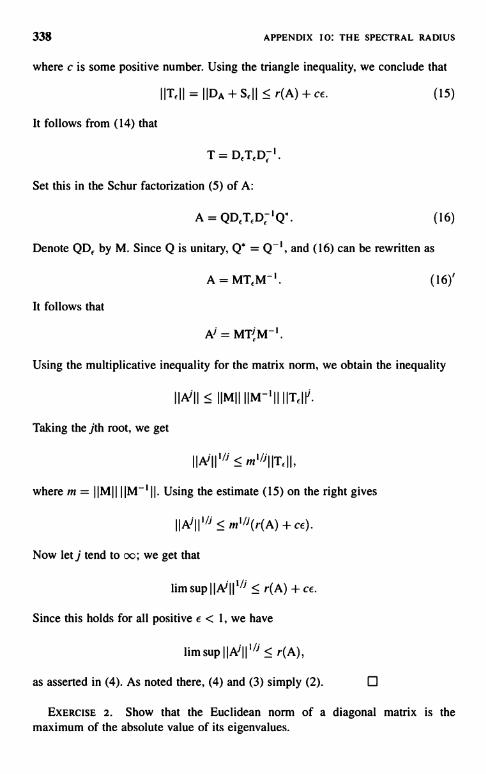
338 APPENDIX TO: THE SPECTRAL RADIUS
where c is some positive number. Using the triangle inequality, we conclude that
IIT,II = IIDA+S,1I < r(A)+cc. (15)
It follows from (14) that
T = D,T,D('.
Set this in the Schur factorization (5) of A:
A = QD,TD,'Q". (16)
Denote QD, by M. Since Q is unitary, Q* = Q-', and (16) can be rewritten as
A=MT,M-'. (16)'
It follows that
Al = MT-M-'.
Using the multiplicative inequality for the matrix norm, we obtain the inequality
I IA'I I <_ I IMI I IIM-' I I I IT,I I'.
Taking the jth root, we get
IIA'II"' < m'/"IIT,II,
where m = IIMII IIM-1 II. Using the estimate (15) on the right gives
IIA'II'/' < m"i (r(A) + cc).
Now let j tend to oo; we get that
lim sup I IA''I 111'' < r(A) + cc.
Since this holds for all positive e < 1, we have
lim sup I IA'II "' < r(A),
as asserted in (4). As noted there, (4) and (3) simply (2).
EXERCISE 2. Show that the Euclidean norm of a diagonal matrix is themaximum of the absolute value of its eigenvalues.
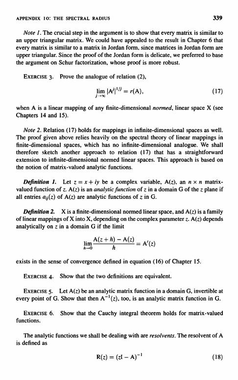
APPENDIX 10: THE SPECTRAL RADIUS 339
Note 1. The crucial step in the argument is to show that every matrix is similar toan upper triangular matrix. We could have appealed to the result in Chapter 6 thatevery matrix is similar to a matrix in Jordan form, since matrices in Jordan form areupper triangular. Since the proof of the Jordan form is delicate, we preferred to basethe argument on Schur factorization, whose proof is more robust.
EXERCISE 3. Prove the analogue of relation (2),
lim IA'I 'l1 = r(A), (17)j-.x
when A is a linear mapping of any finite-dimensional normed, linear space X (seeChapters 14 and 15).
Note 2. Relation (17) holds for mappings in infinite-dimensional spaces as well.The proof given above relies heavily on the spectral theory of linear mappings infinite-dimensional spaces, which has no infinite-dimensional analogue. We shalltherefore sketch another approach to relation (17) that has a straightforwardextension to infinite-dimensional normed linear spaces. This approach is based onthe notion of matrix-valued analytic functions.
Definition I. Let z = x + iy be a complex variable, A(z), an n x n matrix-valued function of z. A(z) is an analytic function of z in a domain G of the z plane ifall entries of A(z) are analytic functions of z in G.
Definition 2. X is a finite-dimensional normed linear space, and A(z) is a familyof linear mappings of X into X, depending on the complex parameter z. A(z) dependsanalytically on z in a domain G if the limit
limA(z + h) - A(z) =
A'(z)n-o h
exists in the sense of convergence defined in equation (16) of Chapter 15.
EXERCISE 4. Show that the two definitions are equivalent.
EXERCISE 5. Let A(z) be an analytic matrix function in a domain G, invertible atevery point of G. Show that then A-' (z), too, is an analytic matrix function in G.
EXERCISE 6. Show that the Cauchy integral theorem holds for matrix-valuedfunctions.
The analytic functions we shall be dealing with are resolvents. The resolvent of Ais defined as
R(z) = (zI - A)-' (18)
340 APPENDIX TO: THE SPECTRAL RADIUS
for all z not an eigenvalue of A. It follows from Exercise 5 that R(z) is an analyticfunction.
Theorem 2. For IzI > JAI R(z) has the expansion
0C AnR(z) = E . (19)0
Proof. By the multiplicative estimate IA" < IAA", it follows that the series on theright-hand of (19) converges for IzI > JAI.
Multiply (19) by (zI - A); term-by-term multiplication gives I on the right-handside. This proves that (19) is the inverse of (zI - A).
Multiply (19) by z' and integrate it over any circle IzI = s > IAA. On the right-hand side we integrate term by term; only the jth integral is # 0, so we get
I R(z)z' dz = 27riA'. (20)
I:1=S
Since R(z) is an analytic function outside the spectrum of A, we can, according toExercise 6, deform the circle of integration to any circle of radius.s=r(A)+e,e>0:
J R(z)z' dz = 27riAA. (20)'
11-1=r(A)+c
To estimate the norm of A! from its integral representation (20)', we rewrite the dzintegration in terms of dO integration, where 0 is the polar angle, z = se'0 anddz = sie'0 d6:
27r
Ai = 1 R(se10)ss+Ie'o(i+')dO.27r
0
(21)
The norm of an integral of linear maps is bounded by the maximum of the integrandtimes the length of the interval of integration. Since R(z) is an analytic function, it iscontinuous on the circle IzI = r(A) + e, e > 0; denote the maximum of IR(z)I onthis circle by c(c). We can then estimate the norm of A' from its integralrepresentation (21), with s = r(A) + e, as follows:
IAII < (r(A) + er+'c(e)

APPENDIX 10: THE SPECTRAL RADIUS 341
Take the jth root:
jAJj"i < m(f)"j(r(A) + f), (22)
where m(f) = (r(A) + f) c(e). Let j tend to oc in (22); we get
lim sup jA'I" < r(A) + f.
Since this holds for all positive f, no matter how small,
lim sup IAAI ""i < r(A).
On the other hand, analogously to (3),
jA'I > r(AY
for any norm. Taking the jth gives
IA'I"' > r(A).
Combining this with (21), we deduce (17).
This proof nowhere uses the finite dimensionality of the normed linear space onwhich A acts.

APPENDIX 1 1
The Lorentz Group
1. In classical mechanics, particles and bodies are located in absolute, motionlessspace equipped with Euclidean structure. Motion of particles is described by givingtheir position in absolute space as a function of an absolute time.
In the relativistic description, there is no absolute space and time, because spaceand time are inseparable. The speed of light is the same in two coordinate systemsmoving with constant velocity with respect to each other. This can be expressed bysaying that the Minkowski metric t2 - x2 - y2 - z2 is the same in both coordinatesystems-here we have taken the speed of light to have the numerical value 1.
A linear transformation of four-dimensional space-time that preserves thequadratic form t2 - x2 - y2 - z2 is called a Lorentz transformation. In this chapterwe shall investigate their properties.
We start with the slightly simpler (2 + 1)-dimensional space-time. Denote by uthe space-time vector (t, x, and denote by M the matrix
1 0 0M= 0 -1 0 (1)
0 0 -1
Clearly,
t2 - x2 - y2 = (u, Mu), (2)
where (,) denotes the standard scalar product in l .
The condition that the Lorentz transformation L preserve the quadratic form (2) isthat for all u,
(Lu, MLu) = (u, Mu)
Linear Algebra and Its Applications. Second Edition, by Peter D. LaxCopyright 2007 John Wiley & Sons, Inc.
(3)
342

APPENDIX II: THE LORENTZ GROUP
Since this holds for all a, v, and u + v, it follows that
(Lu, MLv) = (u, Mv)
343
(3)'
for all pairs u, v. The left-hand side can be rewritten as (u, L'MLv); since (3)' holdsfor all u and v, we conclude that
L'ML = M. (4)
Take the determinant of (4); using the multiplicative property of determinants,along with the fact that det M = 1, we get
(det L') (del L) = (det L)2 = 1.
This shows that every Lorentz transformation is invertible.
EXERCISE I. Show that if L is a Lorentz transformation, so is U.
(4)'
The Lorentz transformations form a group. For clearly, the composite of twotransformations that preserve the quadratic form (2) also preserves (2). Similarly, ifL preserves (2), so does its inverse.
A 3 x 3 matrix has nine elements. Both sides of (3)' are symmetric 3 x 3matrices; their equality imposes six conditions on the entries of L. Therefore,roughly speaking, the Lorentz group forms a three-dimensional manifold.
Definition. The forward light cone (flc) is the set of points in space-time forwhich t2 - x2 - y2 is positive, and t is positive. The backward light cone (blc)consists of points for which t2 - x2 - y2 is positive and t is negative.
Theorem 1. A Lorentz transformation L either maps each light cone onto itselfor onto each other.
Proof. Take any point, say (1, 0, 0)' in the flc; since L preserves the Minkowskimetric (2), the image of this point belongs to either the forward or backward lightcone, say the flc. We claim that then L maps every point a in the tic into the flc. Forsuppose on the contrary that some point u in the flc is mapped by L into the blc.Consider the interval connecting (1. 0, 0)' and u; there would be some point v on thisinterval that is mapped by L into a point w whose t-component is zero. For such apoint w, (w, Mw) < 0. Since all point v on this interval lies in the flc (v, Mv) > v. Butw = Lv, a contradiction to (3).
We show next that every point z in the flc is the image of some point a in the flc.For, since L is invertible, z = Lu for some u; since L preserves the quadratic form(2), u belongs to one of the light cones. If it were the backward light cone. then by theaigument given above L would map all points of the blc into the flc. But L maps(-1, 0, 0)' into -L(l, 0, 0)', which lies in the blc, a contradiction.
APPENDIX I I: THE LORENTZ GROUP
If L maps (1, 0, 0)' into the blc, we argue analogously; this completes the proof ofTheorem 1.
Definition. It follows from (4)' that det L = ± 1. The Lorentz transformationsthat map the tlc onto itself, and for which det L = 1, form the proper Lorentz group.
Theorem 2. Suppose L belongs to the proper Lorentz group, and maps the pointe = (1, 0, 0) onto itself. Then L is rotation around the t axis.
Proof. Le = e implies that the first column of L is (1, 0, 0)'. According to (4),L'ML = M; since Me = e, L'e = e; therefore the first column of L' is (1, 0, 0)'. Sothe first row of L is (1, 0, 0). Thus L has the form
l 0 0
L= 0
0 R
Since L preserves the Minkowski metric, M is an isometry. Since detL= 1,detM = 1; so R is a rotation.
EXERCISE 2. Show that Lorentz transformations preserve solutions of the waveequation. That is, if f (t, x, y) satisfies
then f(L(t,x, y)) satisfies the same equation.
Next we shall present an explicit description of proper Lorentz transformations.Given any point u = (t, x, y)', we represent it by the 2 x 2 symmetric matrix U:
yU_
-(t-x
y t+x
Clearly, U is real and symmetric and
detU=t'--x2-y' trU=2t.
(5)
(6)
Let W be any 2 x 2 real matrix whose determinant equals 1. Define the 2 x 2 matrixV by
WUW' = V. (7)
Clearly, V is real and symmetric and
det V = (det W) (det U) (det W') = det U, (8)
APPENDIX 11: THE LORENTZ GROUP 345
since we have assumed that det W = 1. Denote the entries of V as
r' - x' y'V - y' r' + x'
(9)
Given W, (5), (7), and (9) defines a linear transformation (t,x,y) - (1', X', Y). Itfollows from (6) and (8) that t2 - x2 - y2 = t12 - x12 - y'2. That is, each Wgenerates a Lorentz transformation. We denote it by Lw. Clearly, W and -Wgenerate the same Lorentz transformation. Conversely,
EXERCISE 3. Show that if W and Z generate the same Lorentz transformation,then Z = W or Z = -W.
The 2 x 2 matrices W with real entries and determinant 1 form a group undermatrix multiplication, called the special linear group of order 2 over the reals. Thisgroup is denoted as SL(2, R).
EXERCISE 4. Show that SL(2, R) is connected-that is, that every W in SL(2, R)can be deformed continuously within SL(2, l) into I.
Formulas (5), (7), and (9) define a two-to-one mapping of SL(2, 08) into the(2 + 1)-dimensional Lorentz group. This mapping is a homomorphism, that is,
Lwz = LwLz.
EXERCISE 5. Verify (10).
(10)
Theorem 3. (a) For W in SL(2, R), Lw belongs to the proper Lorentz group.(b) Given any two points u and v in the fic, satisfying (u, Mu) = (v, Mv), there is
a Y in SL(2, lJ) such that Lyu = v.(c) If Z is a rotation, Lz is a rotation around the t axis.
Proof. (a) A symmetric matrix U representing a point it = (t, x, y)' in the flc ispositive, and the converse is also true. For according to (6), det U = t2 - x'- - y2,tr U = 2t, and the positivity of both is equivalent to the positivity of the symmetricmatrix U.
By definitions (7) and (9), the matrix V representing v = Lwu is V = WUW';clearly, if U is a positive symmetric matrix, so is V. This shows that Lw, maps the flcinto the fic.
According to (4)', the determinant of the Lorentz transformation Lw, is 1 or -1.When W is the identity I, Lw, is the identity, and so detLI = 1. During a continuousdeformation of W, det Lw changes continuously, so it doesn't change at all.Therefore, det Lw = 1 for all W that can be deformed continuously into I. According

346 APPENDIX 11: THE LORENTZ GROUP
to Exercise 4, all W can be deformed into I; this shows that for all W, Lw is a properLorentz transformation.
(b) We shall show that given any v in the flc, there is a W in SL(2, l8) such thatLw maps to = t(1, 0, 0)' into v, where t is the positive square root of (v, Mv). Thematrix representing e is I; the matrix representing Lwte is WtIW' = tWW'. So wehave to choose W so that tWW' = V, where V represents v. Since t2 = (V.. MV) =det V and since by (a) V is positive, we can satisfy the equation for W by setting Wasthe positive square root of t-1 V.
Similarly, for any other point u in the flc for which (u, Mu) = (v, Mv), there is a Zin SL(2, u8), for which Lzte = u. Then LwLZ' maps u into v. Since W -+ Lw is ahomomorphism, LwLZ ' = L.
(c) Suppose that Z is a rotation in 1f82; then Z'Z = I. Using the commutativity oftrace, we get from V = ZUZ' that
trV = tr ZUZ' = trUZ'Z = trU
for all U. For U of form (5) and V of form (9), trU = 2t, trV = 2t', sot = t' for al l U.Since t2 - x2 - y2 = t'2 - a12 - y'2, it follows that Lz maps (t, 0, 0) into itself. Weappeal to Theorem 2 to conclude that Lz is rotation around the t axis.
EXERCISE 6. Show that if Z is rotation by angle 0, Lz is rotation by angle 20.
Theorem 4. Every proper Lorentz transformation L is of the form LY Y inSL(2, R).
Proof. Denote by u the image of e = (1,0,0) under L:
Le=u.
Since e lies in the flc, so does u. According to part (b) of Theorem 3, Lwe = u forsome W in SL(2, R). Therefore LWILe = e; according to Theorem 2, LW'L isrotation around the t axis. By part (c) of Theorem 3, along with Exercise 6, thereis a rotation Z in SL(2, J) such that Lw L = Lz; it follows thatL = LwLz = Lwz.
EXERCISE 7. Show that a symmetric 2 x 2 matrix is positive iff its trace anddeterminant are both positive.
EXERCISE 8. (a) Let L(s) be a one-parameter family of Lorentz transformationsthat depends differentiably on s. Show that L(s) satisfies a differential equation of theform
a,L = AML, (11)
where A(s) is anti-self-adjoint.
APPENDIX 11: THE LORENTZ GROUP 347
(b) Let A(s) be a continuous function whose values are anti-self-adjointmatrices. Show that every solution L(s) of (11), whose initial value is I, belongs tothe proper Lorentz group.
2. In this section we shall outline a construction of a model of non-Euclideangeometry using the Lorentz group. By a geometry of the plane, we mean a set ofelements, called points, with the following structures:
(i) a collection of subsets called lines.(ii) a group of motions that map the plane onto itself, and map lines into lines.
(iii) Angles of intersecting lines.
(iv) Distance of pairs of points.
All axioms of Euclidean geometry, except the parallel postulate, have to be satisfied.
Definition. The model, denoted as I-I, consists of the points u located in thepositive half of the hyperboloid
(u, Mu) = t2 - X - y2 = 1, t > 0. (12)
The lines are intersection of 0-0 with planes through the origin (u,p) = 0, wherep satisfies
(p, Mp) < 0. (13)
The group of motions is the proper Lorentz group.
Theorem 5. (a) Every plane (u, p) = 0 that satisfies (13) has a nonemptyintersection with H.
(b) Any two distinct points of 0-0 lie on one and only one line.(c) Every proper Lorentz transformation maps lines onto lines.
Proof. (a) Set p = (s, a, b); condition (13) means that s2 < a2 + b2. The pointu = (a2 + b2, -as, -bs) satisfies (u, p) = 0. We claim that it belongs to the tic; for
(u, Mu) = (a2 + b2)2 - (a2 + b2)s2
is positive, and so is a2 + b2. It follow that u/k, where k is the positive square root of(u, Mu), belongs to H.
(b) Conversely, suppose that the plane (u, p) = 0, p = (s, a, b), contains a pointu = (t, x, y) that belongs to the tic; then p satisfies (13). For suppose not-that is,s2 > a22 + b2. Since u = (t, x, y) belongs to the fic, we have t2 > x2 + y2.Multiplying these inequalities gives
s2t2 > (a2 + b2)(x2 + y2).
348 APPENDIX 11: THE LORENTZ GROUP
Since (u,p) = 0,
St = -(ax + by)
Applying the Schwarz inequality on the right gives the opposite of the previousinequality, a contradictions.
Given two distinct points u and v in 1-0, there is a unique p, except for a constantmultiple, that satisfies (u, p) = 0, (v, p) = 0. According to what we have shownabove, p satisfies (13) when u or v belongs to H.
(c) Take the line consisting of all points u in 0-0 that satisfy (u, p) = 0, where p isa given vector, (p, Mp) < 0. Let L be a proper Lorentz transformation; the inverseimage of the line under L consists of all points v such that u = Lv. These points vsatisfy (Lv,p) = (v, Lp) = 0. We claim that the points v lie on H, and that q = Lpsatisfies (q, Mq) < 0. Both of these assertions follow from the properties of properLorentz transformations.
Next we verify that our geometry in non-Euclidean. Take all lines (u,p) = 0through the point u = (1, 0, 0). Clearly, such a p is of the form p = (0, a, b), and thepoints u = (t, x, y) on the line (u, p) = 0 satisfy
ax + by = 0. (14)
T a k e q = (l , 1, 1); points u = (t, x, y) on the line (u, q) = 0 satisfy t + x + y = 0.For such a point u,
(u, Mu) = t2 - x2 - y2 = (x + y)2 - x2 - y2 = 2xv. (15)
The points u on the intersection of the two lines satisfy both (u,p) = 0and (u, q) = 0. If a and b are of the same sign, it follows from (14) that x and yare of the opposite sign; it follows from (15) that such a u does not lie in theflc.
Thus there are infinitely many lines through the point (1, 0, 0) that do not intersectthe line t + x + y = 0 in 0-0; this violates the parallel postulate of Euclideangeometry.
In our geometry, the proper Lorentz transformation are the analogues ofEuclidean motion translations combined with rotations. Both objects form a three-parameter family.
We turn now to the definition of distance in our geometry. Take two nearbypoints in Oil, denoted as (t, x, y) and (t + dt, x + dx, y + dy). Their image undera proper Lorentz transformation L is (t', x, y') and (t' + dt', x' + dx', y' + dy').Since L is linear, (dt', dx', dy') is the image of (dt, dx, dy) under L, andtherefore
dt2 - dxi2 - dye = dt2 - dx2 - dye,

APPENDIX 11: THE LORENTZ GROUP 349
an invariant quadratic form. Since for points of 0-0, t2 - x2 - yz = 1, we havedt = i dx + ? dy. So we choose as invariant metric
dx'- + dyz - dtz =I
rzyz
dxz + Iz
dyz -2l y
dxdy. (16)
Once we have a metric, we can define the angle between lines at their point ofintersection using the metric (16).
3. In this section we shall briefly outline the theory of Lorentz transformations in(3+1)-dimensional space-time. The details of the results and their proofs areanalogous to those described in Section 1.
The Minkowski metric in 3 + I dimensions is t2 - xz - y' - zz, and a Lorentztransformation is a linear map that preserves this metric. The Minkowski metric canbe expressed, analogously with (2), as
(u, Mu), (17)
where M is the 4 x 4 diagonal matrix whose diagonal entries are 1, -1, -1, and -1,and u denotes a point (t, x, y, z)' in (3 + 1)-dimensional space-time. The forwardlight cone is defined, as before, as the set of points u for which (u, Mu) > 0 andt>0.
A Lorentz transformation is represented by a matrix L that satisfies the four-dimensional analogue of equation (4):
L'ML = M. (18)
A proper Lorentz transformation is one that maps the flc onto itself andwhose determinant det L equals 1. The proper Lorentz transformations form agroup.
Just as in the (2 + 1)-dimensional case, proper Lorentz transformations in 3 + 1space can be described explicitly. We start by representing vectors u = (t, x, y, z)' in3 + I space by complex-valued self-adjoint 2 x 2 matrices
U= (t-x y+iz)y - iz t +x J (19)
The Minkowski metric of it can be expressed as
tz - xz - yz - zz = det U. (20)
Let W be any complex-valued 2 x 2 matrix of determinant 1. Define the 2 x 2matrix V by
V = WUW*, (21)
350 APPENDIX 11: THE LORENTZ GROUP
where W* is the adjoint of W, and U is defined by (19). Clearly, V is self-adjoint, so itcan be written as
V= r'-x, y'+iz' (22),Y -iz' t'+X'
given W, (19), (21), and (22) define a linear map (t, x, y, z) (t', x', y',z'). Take the
determinant of (21):
detV = (detW)(detU)(detW*).
Using (20), (20)', and det W = 1, it follows that
t2-x2-y2-Z2=(2-X'2-y'2-Z12.
This shows that each W generates a Lorentz transformation. We denote it as Lw.The complex-valued 2 x 2 matrices of determinant 1 form a group denoted as
SL(2, Q.
Theorem 6. (a) For every W in SL(2, C), Lw defined above is a proper Lorentztransformation.
(b) The mapping W -> Lw is a homomorphic map of SL(2, C) onto the properLorentz group. This mapping is 2 to 1.
We leave it to the reader to prove this theorem using the techniques developed inSection 1.
4. In this section we shall establish a relation between the group SU(2, C) of 2 x 2unitary matrices and SO(3, 1:8), the group of rotations in P3.
We represent a point (x, y, z)' of R3 by the 2 x 2 matrix
x y+izY - iz -x = U. (23)
Clearly,
- det U = x2 + y2 + z2. (24)
The matrices U are 2 x 2 self-adjoint matrices, trace of U = 0.
Theorem 7. Z is a 2 x 2 unitary matrix of determinant 1, and U is as above.Then
V = ZUZ' (25)

APPENDIX II: THE LORENTZ GROUP 351
is
(i) self-adjoint,(ii) det V = det U,(iii) tr V = 0.
Proof. (i) is clearly true. To see (ii) take the determinant of (25). To deduce (iii),we use the commutativity of trace-that is, that tr AB = tr BA. Thus
trV =trZUZ* =trUZ*Z=trU=0;
here we have used the fact that Z*Z = I for Z unitary.
Combining (23), (24), and (25) shows that the mapping U -> V defined by (25)engenders an orthogonal transformation of W. We denote it as OZ.
The mapping defined by (25) is analogous to the mapping of SL(2, C) onto the(3 + 1)-dimensional proper Lorentz group described in Section 3.
Theorem 8. The mapping Z -> Oz defined above is a homomorphic map ofSU(2, C) onto SO(3, R). This mapping is 2 to 1.
We leave it to the reader to prove this theorem.
We shall now show how to use this representation of rotation in l to rederiveEuler's theorem (see Section 1 of Chapter 11) that every rotation in three space isaround a uniquely defined axis. Representing the rotation as in (25), we have to showthat given any 2 x 2 unitary matrix, detZ = 1, there is a self-adjoint 2 x 2 matrix U,tr U = 0, that satisfies
ZUZ* = U.
Multiplying this relation by Z on the right, we get ZU = UZ. To find a U thatcommutes with Z, we use the eigenvector e and f of Z. They are orthogonal andsatisfy, since det Z = 1,
Ze=.ke, Zf=Xf, IXI=1.
Define U by setting
Ue = e, Uf = f .
Clearly, U is self-adjoint; since its eigenvalues are 1 and -1, tr U = 0. The axis ofrotation consists of all real multiples of U.
APPENDIX 12
Compactness of the Unit Ball
In this Appendix we shall present examples of Euclidean spaces X whose unit ball iscompact-that is, where every sequence {xk} of vectors in X, 11 xk 11 < 1, has aconvergent subsequence. According to Theorem 17 of Chapter 7, such spaces arefinite dimensional. Thus compactness of the unit ball is an important criterion forfinite dimensionality.
Let G be a bounded domain in the x, y plane whose boundary is smooth. Letu(x, ),) be a twice differentiable function that satisfies in G the partial differentialequation
au+Au=0,
where a is a positive constant, and A is the Laplace operator:
Au = u. + uXY;
(1)
(2)
here subscripts x, y denote partial derivatives with respect to these variables.Denote by S the set of solutions of equation (1) which in addition are zero on the
boundary of G:
u(x,y) = 0 for(x,y)in 8G.
Clearly, the set S of such solutions form a linear space.We define for u in S the norm
(3)
IIu1122 = Ju2(x,y). (4)G
Linear Algebra and Its Applications. Second Edition, by Peter D. LaxCopyright ri; 2007 John Wiley & Sons, Inc.
352

APPENDIX 12: COMPACTNESS OF THE UNIT BALL
Theorem 1. The unit ball in S is compact.
Proof. Multiply equation (1) by u and integrate over G:
353
0 =J
(au2 + uAu) dxdy. (5)
G
Using the definition (2) of A, we can integrate the second term by parts:
Ju(uxx+uyy)ddY=_J(u+u)drdY (6)
G
There are no boundary terms resulting from the integration by parts because u is zeroon the boundary of G. Setting (6) into (5), we get
J(u+u)dxdy=aJu2dxdy. (7)
G G
We appeal now to a compactness criterion due to Franz Rellich:
Theorem 2. (Rellich) Let R be a set of smooth functions in a bounded domainG with smooth boundary whose square integrals, along with the square integrals oftheir first derivatives over G, is uniformly bounded:
J U2<m, (8)
G
Every sequence of functions in R contains a subsequence that converges in thesquare integral norm.
The unit ball 11 u 11< 1 in S has the properties (8), since according to inequality(7) the square integral of their first derivatives is bounded by a. So Theorem 1 is aconsequence of Theorem 2.
It follows therefore from Theorem 17 of Chapter 7 that the solutions ofequation (1) that satisfy the boundary conditions (3) form a finite-dimensionalspace.
Theorem 2, and therefore Theorem 1, is not restricted to functions of twovariables or to the specific differential equation (1).
The proof of Rellich's compactness criterion would take us too far afield. But theanalogous result where the square integral norm is replaced by the maximum norm issimpler.

354 APPENDIX 12: COMPACTNESS OF THE UNIT BALL
Theorem 3. Let G be a bounded domain with a smooth boundary, and let D be aset of functions in G whose values and the values of their first derivatives areuniformly bounded in G by a common bound in. Every sequence of functions in Dcontains a subsequence that converges in the maximum norm.
EXERCISE I. (i) Show that a set of functions whose first derivatives areuniformly bounded in G are equicontinuous in G.(ii) Use (i) and the Arzela-Ascoli theorem to prove Theorem 3.

APPENDIX 13
A Characterization of Commutators
We shall prove the following result.
Theorem 1. An n x n matrix X is the commutator of two n x n matrices Aand B,
X = AB - BA,
iff the trace of X is zero.
(1)
Proof We have shown in Theorem 7 of Chapter 5 that trace is commutative-that is, that
tr AB = tr BA.
It follows that for X of form (1), tr X = 0. We show now the converse. i]
Lemma 2. Every matrix X all of whose diagonal entries are zero can berepresented as a commutator.
Proof We shall construct explicitly a pair of matrices A and B so that (1) holds.We choose arbitrarily n distinct numbers at, ... , a,, and define A to be the diagonalmatrix with diagonal entries a;:
1 0 for i#j,ai for i =j.
We define B as
X;jf
Bid= a; - ajor t Ti,
anything for i = j.
Linear Algebra and Its Applications. Second Edition, by Peter D. LaxCopyright 2007 John Wiley & Sons, Inc.
355
356 APPENDIX 13: A CHARACTERIZATION OF COMMUTATORS
Then for i # j
(AB - a;Bij - BJjaj
while
This verifies (1).
= (a1 - aj)B;j = X;j,
(AB - BA)r; = a;B1, - B, a1 = 0.
To complete the proof of Theorem 9 we make use of the observation that if X canbe represented as a commutator, so can any matrix similar to X. This can be seenformally by multiplying equation (1) by S on the left and S-' on the right:
SXS-' = SABS-' - SBAS-'
= (SAS-')(SBS-) - (SBS-')(SAS-' ).
Conceptually, we are using the observation that similar matrices represent the samemapping but in different coordinate systems.
Lemma 3. Every matrix X whose trace is zero is similar to a matrix all whosediagonal entries are zero.
Proof. Suppose not all diagonal entries of X are zero, say x,, 0. Then, sincetr X = 0, there must be another diagonal entry, say x22, that is neither zero nor equalto x,,. Therefore the 2 x 2 minor in the upper left corner of X,
(Xii X12= Y,
x2 x221
is not a multiple of the identity. Therefore there is a vector h with two componentssuch that Yh is not a multiple of h. We introduce now h and Yh as new basis in 082;with respect to this basis Y is represented by a matrix whose first diagonal elementis zero.
Continuing in this fashion we make changes of variables in two-dimensionalsubspaces that introduce a new zero on the diagonal of the matrix representing X,without distroying any of the zeros that are already there, until there are n - 1zeros on the diagonal. But since trX = 0, the remaining diagonal element iszero too.
Combining Lemma 2 and Lemma 3 gives Theorem 1.
APPENDIX 14
Liapunov's Theorem
In this Appendix we give a far-reaching extension of Theorem 20 in Chapter 10. Westart by replacing Z in that result by its negative, W = -Z,
Theorem 1. Let W be a mapping of a finite-dimensional Euclidean space intoitself whose self-adjoint part is negative:
W+W* <0. (1)
Then the eigenvalues of W have negative real part.
This can be proved the same way as Theorem 20 was in Chapter 10. We state nowa generalization of this result.
Theorem 2. Let W be a mapping of a finite-dimensional Euclidean space X intoitself. Let G be a positive self-adjoint map of X into itself that satisfies the inequality
GW + W*G < 0. (2)
Then the eigenvalues of W have negative real part.
Proof Let h be an eigenvector of W, where w is the corresponding eigenvalue:
Wh = wh. (3)
Let the left-hand side of (2) act on h, and take the scalar product with h; accordingto (2),
((GW + W"G)h, h) < 0. (4)
Linear Algebra and Its Applications. Second Edition, by Peter D. LaxCopyright c'! 2007 John Wiley & Sons. Inc.
357

358 APPENDIX 14: LIAPUNOV'S THEOREM
We can rewrite this as
(GWh, h) + (Gh, Wh) < 0.
Using the eigenvalue equation (3), this can be restated as
x(Gh, h) + .(Gh, h) < 0.
We have assumed that G is positive; this means that the quadratic form (Gh, h) ispositive. So we conclude that
A theorem of Liapunov says that the converse of Theorem 2 holds:
Theorem 3 (Liapunov). Let W be a mapping of a finite-dimensional Euclideanspace X into itself, whose eigenvalues have negative real part. Then there exists apositive self-adjoint mapping G such that inequality (2),
GW + W*G < 0, (2)
holds.
Proof. We recall from Chapter 9 the definition of the exponential of a matrix:
Wk00
EewV!
0
(5)
According to Exercise 7 there, the eigenvalues of ew are the exponentials of theeigenvalue of W.
Let t be any real number. The eigenvalues of ew` are e"'', where w is an eigenvalueof W.
Lemma 4. If the eigenvalues of W have negative real part, Iewt I tends to zeroat an exponential rate as t -> +oo.
Proof. According to Theorem 18 of Chapter 7, whose proof appears in Appendix10, for any mapping A of a finite-dimensional Euclidean space X into itself,
lim I I AA II'll= r(A), (6)
where r(A) is the spectral radius of A. We apply this to A = ew. By assumption, theeigenvalues w of W have negative real part. It follows that the eigenvalues of ew,

APPENDIX 14: LIAPUNOV'S THEOREM 359
which are of the form a"', are less than I in absolute value. But then the spectralradius of ew, the maximum of all a", is also less than 1:
r(ew) < 1.
We conclude from (6) applied to A = ew that
I I el I I < (r(ew) + - E
(7)
(8)
where a tends to zero as j oo. It follows from (7) and (8) that Ilew`II decaysexponentially as t oc through integer values.
For t not an integer, we decompose t as t = j +f, where j is an integer and f isbetween 0 and 1, and we factor ew' as
ew` = ewjewf.
So
1 1 ewr 11 <_ 11 el 1I 11 ewf I I (9)
To estimate I I ewf I I we replace in (5) W by Wf,
ewf =
x Wifk
T! '
0
and apply the additive and multiplicative estimates for the norm of a matrix:
X,
IIewf II <_ EIIWkIIJ /^!0
=ell w'llfk!
Since f lies between 0 and 1,
ellwllf < ellw'll. (10)
We can use (8) and (10) to estimate the right-hand side of (9); using j = t - f, weget
Ilewr II < (r+e)`-'elIw1l (11)
where a tends to zero as t -p oo. According to (7), r = r(ew) < 1; thus it follows from(11) that I I ew' I I decays to zero at an exponential rate as t tends to oo.
360 APPENDIX 14: LIAPUNOV'S THEOREM
The adjoint of e" is ev". Since adjoint mappings have the same norm, it followsfrom Lemma 4 that I dew-' I I tends to zero at an exponential rate as t -r cc.
We are now ready to prove Theorem 3 by writing down an explicit formula for G:
00
G = J ew"ew`dt, (12)
0
and verifying that it has the properties required in Theorem 3. But first a word aboutintegrals of functions whose values are mappings:
JA(t)df. (13)
a
There are two ways of defining integrals of form (13), where A(t) is a continuousfunction of t.
Definition 1. Express A(t) as a matrix (a;t(t)) with respect to some basis. Eachof the entries aj(t) is a continuous scalar-valued function, real or complex, whoseintegral is well-defined in calculus.
Definition 2. Form approximating sums
EA(tj)JAjJ; (14)
their limit as the subdivision [a, b] = uAj is refined is the integral (13).
EXERCISE I. Show that the sums (14) tend to a limit as the size of thesubintervals Aj tends to zero. (Hint: Imitate the proof for the scalar case.)
EXERCISE 2. Show that the two definitions are equivalent.
Note. The advantage of Definition 2 is that it can be carried over to infinite-dimensional normed linear spaces.
The integral (12) is over an infinite interval. We define it, as in the scalar case, asthe limit of the integral over [0, T] as T tends to oo.
EXERCISE 3. Show, using Lemma 4, that for the integral (12)
T-aoo
T
limJ
ev"`ew'dt
0
exists.

APPENDIX IQ: LIAPUNOV'S THEOREM 361
We show now that G, as defined by (12), has the three properties required inTheorem 3:
(i) G is self-adjoint.(ii) G is positive.
(iii) GW + W*G is negative.
To show (i), we note that the adjoint of a mapping defined by an integral of the form(13) is
b
JA.(i) dt,
(t
It follows that if the integrand A(t) is self-adjoint for each value of t, then so is theintegral (13). Since the integrand in (12) is self-adjoins, so is the integral G. asasserted in (i).
To show (ii). we make use of the observation that for an integral of form (13) andfor any vector h,
n
(h, JA(t)dth) =J
(h. A(t)h) dt.
It follows that if the integrand A(t) is self-adjoint and positive, so is the integral (13).Since the integrand in (12) is self-adjoint and positive,
(h, ewth)ewth 112 > 0,
so is the integral G. as asserted in (ii). To prove (iii), we apply the factors W and W'under the integral sign:
Xr
OW + W'G =J
(ew.`ew'tW + W'ew"sew') dt. (15)
0
Next we observe that the integrand on the right is a derivative:
Y,ew rewr
To see this, we use the rule for differentiating the product of and e'':
d ewr + d ewrdt (Y,
(16)
(17)

362 APPENDIX 14: LIAPUNOV'S THEOREM
We combine this with the rule for differentiating exponential functions (seeTheorem 5 of Chapter 9):
ewt = ewt W, d ew' = ew,t W` - W'ew..'.dt
Setting these into (17) shows that (16) is indeed the integrand in (15):
xGW + W'G = f (15)'
0
We apply now the fundamental theorem of calculus to evaluate the integral on theright of (15)' as
ew-te% t I'0
Thus we have
GW + W"G = -1,
a negative self-adjoint mapping, as claimed in (iii). This completes the proof ofTheorem 3.
The proof, and therefore the theorem, holds in infinite-dimensional Euclideanspaces.
APPENDIX 15
The Jordan Canonical Form
In this appendix we present a proof of the converse part of Theorem 12 in Chapter 6:
Theorem 1. Let A and B be a pair of n x n matrices with the followingproperties.
(i) A and B have the same eigenvalues ci , ... , ck.(ii) The dimension of the nullspaces
N. (ci) = nullspace of (A - cjI)'
and
Mm(cj) = nullspace of (B - ccI)m
are equal for all c1 and all m:
dimNm(cj) = dimMm(cj).
Then A and B are similar.
(1)
Proof. In Theorem 12 of Chapter 6, we have shown that these conditions arenecessary for A and B to be similar. We show now that they are sufficient byintroducing a special basis in which the action of A is particularly simple anddepends only on the eigenvalues cj and the dimensions (1). We shall deal with eacheigenvalue cl separately; for simplicity we take c = cj to be zero. This can beaccomplished by subtracting cI from A; at the end we shall add cI back.
Linear Algebra and Its Applications, Second Edition, by Peter D. LaxCopyright © 2007 John Wiley & Sons, Inc.
363

364 APPENDIX 15: THE JORDAN CANONICAL FORM
The nullspaces of A' are nested:
where d is the index of the eigenvalue c = 0.
Lemma 2. A maps the quotient space N;+1/Ni into N;/Ni_1, and this mappingis one-to-one.
Proof. A maps N;+1 into N1Ji therefore A maps N;+I /N1 into N;/N;_I. Let {x) bea nonzero equivalence class in N1+I /Nuu; this means that no x belongs to Ni. Itfollows that Ax does not belong to N;_1; this shows that A{x} = {Ax} is not the zeroclass in N;/Ni_,. This proves Lemma 2.
It follows from Lemma 2 that
dim (N1+1 /N1) < dim (Ni/N1-I )
The special basis for A in Nd will be introduced in batches. The first batch,
x1i ...I x1o, l0 = dim (Nd/Nd-1),
(2)
(3)
are any 10 vectors in Nd that are linearly independent mod Nd_I. The next batchis
Ax1,... , Ax,0; (4)
these belong to Nd_ 1, and are linearly independent mod Nd_2. According to (2), withi = d - 1, dim (Nd_I /Nd_2) > dim (Nd/Nd_1) = lo. We choose the next batch ofbasis vectors in Nd_I,
x1o+I,...,xlI, (5)
where 11 = dim (Nd_ I /Nd_2 ), to complete the vectors (4) to a basis of Nd_ 1 /Nd_2.The next batch is
A2 xl,...,A2xb,Axb+1,...,Ax1,. (6)
The next batch,
x1,+1, ... 5 X12, (7)
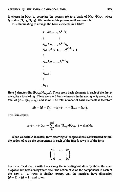
APPENDIX 15: THE JORDAN CANONICAL FORM 365
is chosen in Nd_2 to complete the vectors (6) to a basis of Nd_2/Nd_3, where12 = dim (Nd_2/Nd_3). We continue this process until we reach N1.
It is illuminating to arrange the basis elements in a table:
xl,Axl,...,Ad-lxl
x10, Axl,... , Ad-xla
xlo+1, Axl0+1, , Ad-2xfa+1
Here IJ denotes dim (Nd f/Nd -j_1). There are d basis elements in each of the first lprows, for a total of NO. There are d - 1 basis elements in the next 11 -1o rows, for atotal of (d - 1)(11 - lo), and so on. The total number of basis elements is therefore
d1o+(d- 1)(11 -Id-2)
This sum equals
d-1lo+ +Id-l =E dim (Ndf/Nd f-1) = dim Nd.
0
When we write A in matrix form referring to the special basis constructed before,the action of A on the components in each of the first 10 rows is of the form
al ... 0
0 ... 0
that is, a d x d matrix with 1 - s along the superdiagonal directly above the maindiagonal, but zeros everywhere else. The action of A on the components in each ofthe next 11 - 10 rows is similar, except that the matrices have dimension(d - 1) x (d - 1), and so on.

366 APPENDIX 15: THE JORDAN CANONICAL FORM
Recall that in order to simplify the presentation of the special basis we havereplaced A by A - cl. Putting back what we have subtracted leads to the followingmatrix form of the action of A:
Cl ... 0
1
0 ... C
that is, each entry along the main diagonal is the eigenvalue c, I - s along thesuperdiagonal directly above it, and zeros everywhere else. A matrix of this form iscalled a Jordan block, when all Jordan blocks are put together, the resulting matrix iscalled a Jordan representation of the mapping A.
The Jordan representation of A depends only on the eigenvalues of A and thedimension of the generalized eigenspaces N! (ak), j = 1, ... , dk, k = 1, .... There-fore two matrices that have the same eigenvalues and the same-dimensionaleigenspaces and generalized eigenspaces have the same Jordan representation. Thisshows that they are similar. 11
APPENDIX 16
Numerical Range
Let X be a Euclidean space over the complex numbers, and let A be a mapping of Xinto X.
Definition. The numerical range of A is the set of complex numbers
(Ax, x), IIx11=1.
Note that the eigenvalues of A belong to its numerical range.
Definition. The numerical radius w(A) of A is the supremum of the absolutevalues in the numerical range of A:
w(A) = sup I(A.x, x)I. (I)
Since the eigenvalues of A belong to its numerical range, the numerical radius of Ais > its spectral radius:
r(A) < w(A). (2)
EXERCISE I.
EXERCISE 2.
Show that for A normal, equality holds in (2).
Show that for A normal,
w(A)=IIAII (3)
Linear Algebm and Its Applications. Second Edition, by Peter D. LaxCopyright 4 2(4)7 John Wiley & Sons, Inc.
367
368 APPENDIX 16: NUMERICAL RANGE
Lemma 1. (i) w(A) < 11 A I I
(ii) II A II <_ 2w(A). (4)
Proof. By the Schwarz inequality we have
I(Ax,x)I <_ IIAxII IIxII <_ IIAII IIxII2;
since I I x I I= 1, part (i) follows.(ii) Decompose A into its self-adjoint and anti-self-adjoint parts:
A=S+iT.
Then
(Ax, x) = (Sx, x) + i(Tx, x)
splits (Ax, x) into its real and imaginary parts; therefore
I(Ax, x) I > (Sx, x), I(Ax, x)I > (Tx, x).
Taking the supremum over all unit vectors x gives
w(A) > w(S), w(A) > w(T).
Since S and T are self-adjoint,
w(S) = I I S II, w(T) =IITII
Adding the two inequalities (5), we get
2w(A)>IISII+IITII
Since IIAII <_ I I S + I I T 11, (4) follows.
Paul Halmos conjectured the following:
Theorem 2. For A as above,
w(A") < w(A)"
(5)
(6)
for every positive integer n.
APPENDIX 16: NUMERICAL RANGE 369
The first proof of this result was given by Charles Berger. The remarkable simpleproof presented here is Carl Pearcy's.
Lemma 3. Denote by rk, k = 1, ... , n, the nth roots of unity: rk = e2ilkl". Forall complex numbers z,
1-z"=11 (1-rkz),k
and
1=1E j(1-rkz).1 k#j
EXERCISE 3. Verify (7) and (8).Set A in place of z, we get
I-A"=11 (I - rkA)
and
I=IEjj(I-rkA).j k#j
Let x be any unit vector, I I x I I = 1; denote
(7)
(8)
(9)
(10)
(I - rkA)x = xj. (11)k&j
Letting (9) act on x and using (11), we get
x - A"x = (I - rjA)xj, j=1,...,n. (12)
From (10) acting on x, we get
X=I-nExj.
Take the scalar product of (12) with x; since I I x I I = 1, we get on the left
(13)
I-(A"x, x)=(x-A"x, x)=n(x-A"x,Exj); (14),
370 APPENDIX 16: NUMERICAL RANGE
in the last step we have used (13). Next use (12) on the right:
By the definition of w(A),
(14)2
I(Axj,xj)1 :5 w(A)IIxj112. (15)
Suppose that w(A) < 1. Then, since I rji = 1, it follows from (15) that the real part of(14)2 is nonnegative. Since (14)2 equals (14)1, it follows that the real part of1 - (Ax, x) is nonnegative.
Let w be any complex number, Iwl = 1. From the definition of numerical radius, itfollows that wu(wA) = w(A); therefore, by the above argument, if w(A) < 1, weobtain
I - Re(w"A"x, x) = 1 - Rew"(A"x, x) > 0.
Since this holds for all w, jwj = 1, it follows that
I(A"x, x)I < 1
for all unit vectors x. It follows that w(A") < 1 if w(A) < 1.Since w(A) is a homogeneous function of degree 1,
w(zA) = Izlw(A),
and conclusion (6) of Theorem 2 follows.
Combining Theorem 2 with Lemma 1, we obtain the following:
Corollary V. Let A denote an operator as above for which w(A) < 1. Then forall n, we have
IIA"II<2. (16)
This corollary is useful for studying the stability of difference approximations ofhyperbolic equations.
Note 1. The proof of Theorem 2 nowhere makes use of the finite dimensionalityof the Euclidean space X.
Note 2. Toeplitz and Hausdorff have proved that the numerical range of everymapping A is a convex subset of the complex plane.
EXERCISE 4. Determine the numerical range of A = (o 1) and of A2 = ( I).
APPENDIX t6: NUMERICAI. RANGE 371
BIBLIOGRAPHY
Halmos, P. R. A Hilherr Space Problem Book. Van Nostrand, New York. 1967.
Lax, P. D., and Wendroff, B. Difference schemes for hyperbolic equations with high order ofaccuracy, CPAM 17 (1964). 381-398.
Lax, P. D., and Nirenberg. L. On stability for difference schemes: a sharp form of Garding'sinequality. CPAM 19 (1966), 473-492.
Pearcy, C. An elementary proof of the power inequality for the numerical radius. MichiganMath. J. 13 (1966), 289-291.


Index
Adjoint, 84, 85Annihilator, 15Arzela-Ascoli, 354Avoidance of crossing, 141
Basis, 5ordered, 326orthonormal, 80
Bellman xiv, 240Bohnenblust, 240Bounded set, 195
Caratheodory's theorem, 195Cauchy:
matrix, 308sequence, 92
Cayley-Hamilton theorem, 67Cayley's Theorem, 305Characteristic polynomial, 61, 63Characterstic value see EigenvalueChebyshev:
iteration, 252polynomial, 253
Closed set, 193, 218Codimension, 16Commutator, 355Commuting maps, 74Compactness of unit ball, 352Compactness local, 92, 93Completeness, 92
Condition number, 248Conjugate gradient, 246, 256Convergence, 92
rate of, 252, 254, 260Convex set, 187
extreme point, 195gauge function, 188hull, 194interior point, 188support function, 193
Cooley, 333Coset see Quotient spaceCross product, 99
Deift, 269, 276Determinant, 45, 65
Cauchy, 303Cramer's rule, 54integral formula for, 157Laplace expansion, 52multiplicative property of, 49of positive matrices, 154, 156Vandermonde, 302
Difference equations, 23Differential equations, see VibrationDifferentiation:
of determinant, 127rules of, 122
Dimension, 5codimension, 16
Linear Algebra and Its Applications, Second Edition, by Peter D. LaxCopyright © 2007 John Wiley & Sons, Inc.
373
374
Domain space, 19Dot product, see Scalar productDoubly stochastic matrix, 197Dual:
lattice, 318norm, 221, 231space, 14
Duality theorem, 206economics interpretation of, 208
Eigenvalue, 59, 60, 262of anti-selfadjoint map, 112index, 72multiple, 68of selfadjoint map, 106simple, 129smallest largest, 113, 114, 166of unitary map, 113variational characterization, 113
Eigenvector, 59, 60expansion, 64generalized, 69
Energy see vibrationError, 248Euclidean structure, 79
complex, 95Euler's theorem, 172Exponential function, 111, 127, 128
Farkas-Minkowski theorem, 203Fast matrix multiplication, 320Fast Fourier transform, 328Fibonacci sequence, 62Finite Fourier transform, 119, 328Fischer, 116Flaschka, 269Fluid flow, 177
curl, 179divergence, 180
Francis, 263Frequency, 180Friedland, Robbin and Sylvester, 327Frobenius theorem, 243Function of selfadjoint mappings, I l l
analytic, 140monotone, 151
Fundamental theorem, 20
Game theory, 209min max theorem, 210
Gauge function, 188Gauss, 246
Gaussian elimination, 39Gershgorin's theorem, 323Givens, 246, 269Google, 242Gram matrix, 152, 316Gram-Schmidt procedure, 81
Hadamard, 157Hahn-Banach theorem, 191
complex version, 226Halmos-Berger-Pearcy, 369Hamiltonian equation, 312Helly's theorem, 199Herglotz, 152Hermitean symmetric, 101Hestenes, 246Hilbert-Schmidt norm, 99Holder inequality, 215Householder, 246, 266Hyperplane, 187
separation theorem, 190, 192
Inner product, see Scalar productInterpolation, 22Inverse, 25
Isometry, See also orthogonaland unitary matrix, 87
Isomorphism, 3Iteration:
Chebyshev, 252, 253conjugate gradient, 256iterative methods, 248steepest descent, 249
Jacobi, 246Jacobian, 177Jordan form xii, 366
Konig-Birkhoff theorem, 198Krein-Milman theorem, 199
Lanczos, 246Lattice, 317
dust, 318integer basis, 318
Law of Inertia, 105Lax, 325Liapunov's Theorem, 358
INDEX
INDEX
Linear:bilinear, 79combination, 4dependence, 5function, 13independence,5operator, 20space, 1subspace, 4system of equations, 39transformation, 20
Linear mapping(s), 19algebra of, 24invertible, 25, 233norm of, 89, 230transpose of, 26
Loewner, 151Lorentz
group, 343transformation, 342
Matrix, 33anti-selfadjoint, 112block, 38column rank, 37diagonal, 38Gram, 152, 316Hermitean, 101Hessian, 102identity, 38Jacobian, 177multiplication of, 34, 35, 320normal, 112orthogonal, 89positive, 237positive selfadjoint,
117, 143row rank, 37selfadjoint, 101similar, 38symmetric, 101symplectic, 309transpose, 36tridiagonal, 38unimodular, 318unitary, 96valued function, 122
Minimal polynomial, 72, 73Minmax principle, 116, 118
of game theory, 210Monotonic matrix function, 151Minkowski metric, 342, 349Moser's Theorem, 273Muraki, 142
Nanda, 269Non-Euclidean geometry, 347Norm(s), 89
equivalent, 217Euclidean, 79dual, 90of mapping, 230of matrix, 89
Normal mode, 184Nonmed linear space, 214
complex, 225Nullspace, 20Numerical
radius, 367range, 367
Orientation, 44Orthogonal, 80
complement, 82group, 89matrix, 89, 108projection, 83
Orthonormal basis, 80
Parallelogram law, 227Permutation, 46
group, 34, 46matrix, 197signature of, 47
Person's theorem, 237Pfaffian, 305Polar decomposition, 169Polynomial,
characteristic, 61, 63minimal, 72
Population evolution, 242Positive definite, see Positive
selfadjointPositive selfadjoint mapping, 117, 143Principal minor, 131, 162Projection, 30
orthogonal, 110Phythagorean theorem, 80
375
376
QR algorithm, 263Quadratic form, 102
diagonal form, 103Quadrature formula, 17Quotient space, 8
nonmed, 225
Random, 200Range, 20Rank see row and column rankRayleigh quotient, 114Reflection, 89, 226Rellich's theorem, 140, 353Residual, 249Resolution of the identity, 110Riesz, F, 152, 220Rigid motion, 172
angular velocity vector, 176infinitesimal generator, 174
Rotation, 172Rounding, 247
Scalar, 2Scalar product, 77, 79Schur factorization, 335Schur's theorem, 153, 316Schwarz inequality, 79Selfadjoint, 106
anti-selfadjoint, 112part, 112
Similarity, 29, 55Simplex, ordered, 44Singular value, 170Solving systems of linear equations,
Chebyshev iteration, 252optimal three-term iteration, 256steepest descent, 249three-term Chebyshev
iteration, 255Gaussian elimination, 39
Spectral Theorem, 70of commuting maps, 74mapping theorem, 66redius, 97, 334resolution, 110of selfadjoint maps, 106
Spectrum of a matrix:anti-selfadjoint, 112orthogonal, 86, 113
selfadjoint, 106symplectic, 309unitary, 113
Square root of positive matrix, 145Steepest descent see iterationStiefel, 246Stochastic matrix, 240Strassen, 320Subspace, 4distance from, 84, 223Support function, 193Symmetrized product, 148Symplectic matrix, 309
group, 309
Target space, 19Tensor product, 313Toda flow, 269Tomei, 269Trace, 55, 65Transpose:
of linear map, 26of matrix, 36
Triangle inequality, 80, 215Tukey, 333
Underdetermined systems of linearequation, 21
Unitary:map, 96group, 96
Vandermonde matrix, 302determinant, 302
Vector, 1norm of, 79, 214valued function, 121
Vector space see Linear spaceViberation, 180
amplitude, 180, 182energy, 180, 182frequency of, 180phase, 180
Volume, 44Signed, 45
von Neumann, 213, 246and Wigner, 141
Wieland-Hoffman theorem, 164
INDEX
PRAISE FOR THE FIRST EDITION
I,, ;or gluduate
- i;c mofhemetiiitrn s bot}kshell."
-Ialli L'r,'l`li!I JIiIvll rii17rJi of
Linear Algebra and rrs Applications, Second fair ion presents linear algebra as the theory andpractice of linear spaces and linear maps with a unique focus on the analytical aspects as well asthe numerous applications of the subject. In addition to thorough coverage of linear equations,matrices, vector spaces. game theory. and numerical analysis. the Second Edition features student-friendly additions that enhance the book's accessibility, including expanded topical coverage inthe early chapters, additional exercises, and solutions to selected problems.
Beginning chapters are devoted to the abstract structure of finite dimensional vector spaces, andsubsequent chapters address convexity and the duality theorem as well as describe the basicsof normed linear spaces and linear maps between Wormed spaces.
Further updates and revisions have been included to reflect the most up-to-date coverage of thetopic. including:
The QR algorithm for finding the eigenvalues of a self-adjoint matrix
The Householder algorithm for turning self-adjoins matrices into tridiagonal Form
The compactness of the unit ball as a criterion of finite dimensionality of a normed linear space
Additionally, eight new appendices have been added and cover topics such as: the Fast FourierTransform; the spectral radius theorem; the Lorentz group; the compactness criterion for finitedimensionality, the characterization of commentators; proof of Liapunods stability criterion; theconstruction of the Jordan Canonical form of matrices: and Carl Pearcy's elegant proof of Halmos'conjecture about the numerical range of matrices.
Clear. concise. and superbly organized, Linear Algebra and Its Applications, Second Edition servesas an excellent text for advanced undergraduate- and graduate-level courses in linear algebra. Itscomprehensive treatment of the subject also makes it an ideal reference or self-study for industryprofessionals.
PETER D. LAX, PHD, is Professor Emeritus of Mathematics at the Courant Institute ofMathematical Sciences at New York University. Dr. Lax is the recipient of the Abel Prize for 2005 "forhis groundbreaking contributions to the theory and application of partial differential equations andto the computation of their solutions. * A student and then colleague of Richard Courant. Fritz John,and K, 0. Friedrichs. he is considered one of the world's leading mathemat cians, He has had a longand distinguished career in pure and applied mathematics. and with over fifty years of experience inthe field. he has made significant contributions to various areas of research, including inregratablesystems, fluid dynamics. and solitonic physics, as well as mathematical and scientific computing.
* The Abel Pre 1065 Pest Release
Subscribe to our fray Math ',mitts eNewcIetter atwww.w'ley.corri fenewsletters
ISO" r
i I ' "' .I,, 1-0"t;'-5 ht M3I,C5
WI LEY-1)INTERSCIENCE
I so7WILEY
2007