LIMITING DISTRIBUTION OF THE PRESENT VALUE OF A PORTFOLIO

BY GARY PARKER

Simon Fra~er Umvers'ttv

ABSTRACT

An approximation of the distribution of the present value of the benefits of a portfolio of temporary insurance contracts is suggested for the case where the size of the portfolio tends to infinity. The model used Is the one presented in PARKER (1922b) and involves random interest rates and future hfenmes Some justifications of the approximation are given. Illustrations for hmttmg portfolios of temporary insurance contracts are presented for an assumed Ornstem-Uhlenbeck process for the force of interest

KEYWORDS

Force of interest, Ornsteln-Uhlenbeck process, Portfolio of pohcles; Present value function; Limiting distribution

I . INTRODUCTION

When considering random mterest rates in actuarial funcnons, a question of particular interest is the distribution of the plesent value of a portfolio of policies Studying such distributions could be very useful in areas such as pricing, valuation, solvency analysis and reinsurance.

Some references which considered stochastic interest rates in actuarial functions are BOYLE (1976), W~LKIE (1976), WATERS (1978), PANJER and BELLHOUSE (1980), DEVOLDER ( ] 986), GIACOTTO (1986), DHAENE (1989), DUFRESNE (1988), BEEKMAN and FUELLING (1990), PARKI~R (1992b).

Recently, DUFRESNE (1990) derived the distribution of a perpetuity for i.i d interest rates. FREES (1990) recurswely expressed by an integral equation the distribution of a block of n-year annumes for i i d interest rates.

This paper, taken for the most part from the author's Ph.D thests (PARKER (1992a)), presents an approximation of the hmiting distribution, as the number of policies tend to infinity, of the average present value of the benefits for a specific type of portfolio of insurance contracts Although, theoretically, the approach may be used for any stochastic process for the interest rates, tt is more convenient for Gausslan processes The approximation is justified by two correlation coefficients which happen to be relanvely high mainly because of the defininon of the present value function. Some illustrations of the distribution function of the present value of portfolios using the Ornstem-Uhlenbeck process are presented Finally, the

AST1N BULLETIN. Vol 24. No I. 1994

4 8 GARY PARKER

moments of some approximate distributions are compared with the corresponding exact moments

2. A PORTFOLIO

Consider a portfolio of temporary insurance contracts, each with sum insured 1, issued to c lives insured aged x. Let Z (c ) be the random present value of the benefits of the portfolio

PARKER (1922b) used a definition of 2;(c) involving a summation over the c contracts of the portfolio. That is

c

(2.1) Z ( c ) = ~ Z , , I = l

where Z,, ~s the present value of the benefit for the ith life insured of the portfolio. This definmon ts convement for calculating the moments of Z (c ) because it ms possible to simplify the expressmns for these moments under the assumption that the future lifetimes of the c policyholders are mutually independent.

Another definition which ms eqmvalent appears to be more appropnate for studying the hmltmg distribution of the random variable g ( c ) .

Instead of summing over the c policies, one could consider summing the present value of the benefits in a given year over the n pohcy-years of the contract Algebraically, we have

Iw- 1

Z . , ( c ) = 2 C, e - ' O + l ) , t=o

(2.2)

where

I l + l

(2.3) y (i + 1) = 6, ds, 0

de is the force of interest at time s and c,, : = 0, 1, .. , n - 1 is the random variable denoting the number of pohcms where the death benefit ~s actually paid at time t + 1. We let c,, be the number of lives insured surviving to the end of the term, n Note that the sum of the c, 's from t equal 0 to n is c, the total number of pohcies m the porffoho. Thus,

(24) ~ c, = c I=0

When studying Z,(c), we will assume that the future lifetimes of the lives insured are mutually independent and independent of the forces of interest {d~}~ >_ 0. In this case, the {c,}'/= i is multinominal We will also assume that the discounting of all the benefits for the policies in the portfolios is done with the same Gausslan forces of interest.

In the next sectmn, we consider hmmng portfohos, i.e portfohos where the number of contracts tends to infinity.

L I M I T I N G D I S T R I B U T I O N O F T H E PRESENT V A L U E O F A P O R T F O L I O 49

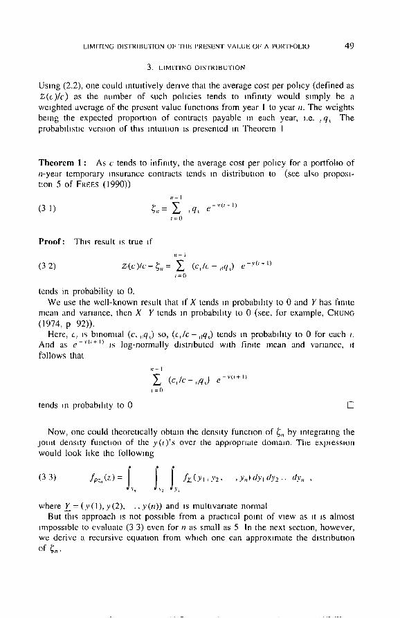
3. L I M I T I N G D I S T R I B U T I O N

Using (2.2), one could lntmtively derive that the average cost per pohcy (defined as Z ( c ) / c ) as the number of such policies tends to mfimty would simply be a weighted average of the present value functions from year I to year n. The weights being the expected propomon of contracts payable m each year, Le. ,~q~ The probabdlstlc version of th~s mtUltton is presented in Theorem I

T h e o r e m 1 : As c tends to infinity, the average cost per policy for a portfoho of n-year temporary insurance contracts tends m distributton to (see also proposi- tion 5 of FREES (1990))

t ; - I

t = 0

P r o o f : This result is true if

n - I

(3 2) Z ( c ) / c - ~ , , = ~ (c,/~ - ,~q,) e -.'~'+ll t = 0

tends in probabili ty to 0. We use the well-known result that if X tends m probabili ty to 0 and Y has fimte

mean and variance, then X Y tends m probabdlty to 0 (see, for example, CHUNG (1974, p 92)).

Here, c, is bmomtal (c, ,,q,) so, ( c , / c - ,,q,) tends m probab,l l ty to 0 for each t. And as e -~'l'+l~ Js log-normally d~stnbuted with fimte mean and varmnce, it follows that

tends m probabdtty to 0

n - I

~ (c,/c-,~qO e t=O

- ' ¢ i : + I)

[]

Now, one could theoretically obtain the density function of ~,, by integrating the jomt density functton of the y ( t ) ' s over the appropriate domain. The expressmn would look hke the following

Ve ~2 YL

where Y=(y(I),y(2), . , y ( n ) ) and is multivariate normal But this approach is not possible from a practical point of view as it is almost

impossible to evaluate (3 3) even for n as small as 5 In the next secuon, however, we derive a recursive equatton from whmh one can approximate the dtstnbut~on of ~..

50 GARY PARKER

4. APPROXIMATION

Since ~,, Is a summation over the policy-years, it is easy to break it down into the sum of ~,_ i and a term for the nth policy year. The recurslve equation for ~,z is then given by :

n - I n - 2

~, '= 2 ,'q, e - " l ' + l ) = 2 ,q, e-" l '+ ' l+, , -J ,q , e - ' ( " ) = 0 ~ = 0

(4.1) ~,, = ~,~_ i + . _ i,q, e - 'u ' l

Let z, be a possible realization of z, and vj be a possible realization of y(j) Let the function g,,(z., y,,). a somewhat unusual function based on the dlstrlbu-

non of ¢,~ and the density function of y(n). be defined as:

(4.2) g,, (z,,, y,,) = P(~,, --< z,,) f,'u,I (y,,l~,, --< z,,),

or equivalently,

(4 3) g,,(z,,, y,,) = f , u,l(Y,,) P(~,, <- z,,ly (n) --.y,).

From this last definition, it fol lows Immediately that the distribution function of ~, is given by:

F ~ . ( z , , ) = [ " g , ( z , , . y , , ) d y e , (4.4) d - ~c

where the funcnon g, (z,, Y,,) may be calculated with a high degree of accuracy from the following recurslve equation

(45) g , , ( z , , , , , , , ) ~ I i ~ f , , , , ) ( y , , l y ( n - l ) = y , , _ , ) x

- - Vn 7 x g , , - i ( z , , - , , - i Jq , e , ) , - i ) d y , , - i

with the starting value '

(46) g j ( z , , y , ) = ~b~ ~ / - i - ~ ) If z,-->q~ e - "

0 otherwise

We use the notation ¢ ( ) to denote the probability density function of a zero mean and un,t variance normal random variable. Note also that given that y ( n - l) equal y,,_ ~, y(n) is normally distributed with mean

(47) E [ y ( n ) t y ( n - l ) = y , , _ t ]

coy (y(n) , y(n - 1)) =Ely(n)] + { .v , , - i -Ely(n-1)1}

Wly(n)l

LIMITING DISTRIBUTION OF THE PRESENT VALUE OF A PORTFOLIO 5 1

and variance

(4.8) V i y ( n ) l y ( n - l ) = y , , _ ~l = Vly(n) l -

( s e e , for example, MORRISON (1990, p . 9 2 ) )

coy 2 ( y ( n ) , y ( n - 1))

V l y ( n - 1)]

To derive (4.5), we start by noting that from ( 4 . 1 ) , we have that"

(49) P(~,, --< z,,ly(n) = y . ) = P(~._ l <- z , , - , ,_ i,q, e-Y"IY(n) =Y.)

Now using (42), (4.3) and (4.9), we have

(4.10) g.(z,~.Y, ,)=P(~,,- i <--z,,-.-i~q, e -y") x

x f~( , )(Y, , l~, , - I--<Zn-, , - t tq , e - " ' )

The conditional probability density function of y(n) In (4.10) may be written as: (MELSA and SAGE (1973, p. 98))

(4.11) f, . t ,)(y,~l~,,_l--<Z,,-, ,-itq, e - " )

= I i ~ f w ' ) ( y ' l y ( n - I ) = Y " - " ~ " - ' < - - z " - " - " q ' e-~") x

x L,(,,_ii ( y , , _ l l ~ . _ ] - ~ z , , - , , - i ~ q ,

Equation (4.3) imphes that

(412) f,,i,,_l)(V,,_ll:£,,_t <--Z,,--,,_llq, e-Y") -

e-"") dy,,_ i .

g , , _ j ( z , , - ,, _ l l q , e - '" . y , , _ i )

P ( ~ ' , _ ] - < z , , - ,, _ J l q , e - " )

If we now make the following approximation (see the next section for some justifications)

(413) f ,~, , )(y , , ly(n-l)=y, ,_~.~, ,_t--<z, , - , ,_~Lq, e .... )_=

--f~ t,,)(y,,ly ( n - I) =y,,_ ,),

then equation (411) becomes

(4 14) f , t , , l(y, , l~._l <-- Z,, - . - t~q, e-"°) ~ f , , ( ,~)(y , , ly(n-1)=y._ 0 x

9 . - i (z,, - . - IIq, e - ' ° . Y,,- i) x dy,,_ I

P(~,,-I <- Z,,-,,-l~q., e -~")

Finally substmltlng this last expression (4.14) into (410), we obtain (45). To obtain the starting value (4.6), we simply have to note that:

-y(1) (415) ~l =q, e

52 GARY PARKER

and that

(4 16)

Then, since (4.17)

we have that

g , (z l ,Y,) = P ( ~ t - < z t l y ( I ) = y , ) f~t,l(V,)

=P(~ ' I - -<z l lv( l )=v , ) . ~p(:v,-Ely(l)])V[3~(li] ~

~,=q, e - " If y ( I ) = y , .

(4 18) P(~l ~ Z i I v ( I ) : Y ' ] ) = I l if zl-->q,e (o otherwise

Finally, by combining (4 18) and (4 16). we obtain (4 6) This completes the derivation of (4 5) and (4.6)

Before doing numerical evaluations of approximation (4.5). it is ,nportant to study In greater details and to justify the approximation (4 13) involved here This is done in the next section.

5. JUSTIFICATIONS

Looking at the steps leading to (4.5), we note that the result ~s not exact due only to approxlmatmn (4.13) made m order to obtain a recurslve equation revolving only known quanutles This approximation may be justified theoretically by looking at two particular correlation coefficients, one of which vahdates the approximation for large values of n and the other for small values of n

5.1 Correlat ion between y (n) and y (n - 1)

From the subject of multivariate analysis, we know that the approximation (4.13) will be acceptable if y(n) and y ( n - I) are highly correlated (see, for example, MARINA, KENT and BmBY (1979, Section 6.5)) This is true since If they are highly correlated, knowing y(n- I) would e×plaln much of y(n). Now if thls is the case, introducing any other variable, correlated or not with v(n), in the regression model to further explain y(n) cannot improve the situation much.

Looking back at the definition ofy(n) (see (2.3)) it is clear that y(n - l) and v(n) must be highly correlated. Their correlation coefficient will be given by: (Ross (1988, p. 280))

coy (y(n), y(n - 1)) (5.1) O(y(n), y ( n - 1 ) ) -

{V[y(n)l V [ y ( n - I ) ] } 1:2

Note that if the force of interest is modeled by a White Noise process, i.e.

(5.2) 6, N(ZI. 2

LIMITING DISTRIBUTION OF THE PRESENT VALUE OF A PORTFOLIO 53

where ~t is understood that its integral, y(t), is a Wiener process, it can be shown that, the expected value of y ( t ) Is

(5 3) E [ y ( t ) l = A t

and ~ts autocovarmnce funcuon ~s

(5 4) cov (y(s ) , y( t ) ) = o,2~, mm (s, t)

If the force of interest i,; modeled by the following Ornstem-Uhlenbeck process.

(5.5) d~t = - o~ (6, - ~) dr + ~ d W , ,

with initial value 6o, then y( t ) has an expected value of

(5.6) E l y ( t ) l = 6 r + ( 6 o - 6 )

a n d its a t t t o c o v a t l a n c e f u n c t i o n is

0 2 (5 7 ) COV ( y ( ~ ) , y ( t ) ) = - - m m ( s , t ) +

o~ 2

O 2 + - - 1 - 2 + 2 e - ~ + 2 e - ~ - e - " l ' - ' ~ - e - " ° + ' ) l

2 ~ 3

(see, PARKER (1922b, equations 38 and 39)) The correlation coefficients between y(n) and y(n - I) for different values of n,

when the force of mtere,,t is modeled by a White Noise (see (5 2)) and when it ts modeled by an Ornstem-Uhlenbeck process (see (5.5)) with parameter o~ = . I, 2 or 5 are presented m Table I

T A B L E I

CORRI:LATION COEI I-ICIEN I BETWEEN V (It) AND y (It -- I ) FORCE O1" IN1EREST AS WHIIL NOIM AND ORNSTEIN-UIILENBFCK PROCESSES

. While Noise Orns tem-Uhlenbcck

t~= I ~ = 2 ~ = 5

2 7071 8773 8707 8516 3 8165 9474 9423 9270 4 8660 9701 9659 95~5 5 8944 9804 9769 9664 6 9129 9860 9829 9739 7 9258 9894 9867 9788 8 9354 9916 9891 9821 9 9428 9931 9909 9846

10 9487 9942 9922 9865 20 9747 9980 9969 9940 40 9874 9992 9987 9972 60 9916 9995 9991 9981

54 GARY PARKER

Results for the White Noise process are presented here because this process involves ~.~ d. forces of interest, therefore, leading to the lowest correlation coefficients Results for the Ornstein-Uhlenbeck process are presented because it ~s the process used for dlustrat~on purposes m the next section.

Note that the correlation coefficient between y(n) and y(n - I) Is not influenced by the parameter o,o of the White Noxse process. For the Omsteln-Uhlenbeck process, the parameter 60, 6 and cr have no incidence on the correlation coefficients

Table 1 clearly shows that y(n) and y ( n - 1 ) are very highly correlated, especmlly for large values of n. Therefore, approximation (4.13) made to obtain the recursive equation (4.5) should be acceptable

Another correlation coefficient could also JUStify approximation (4 13), indepen- dently of the one discussed here This is the subject of the next section.

5.2. Correlation between e-Y~"J and ~.

Again from the subject of multivariate analysis, we know that the approximation (4 13) would also be acceptable ff y(n - I) and ~,,_ ~ contained about the same useful reformation to explain ~,(n) (see, for exemple, MARDIA, KF:NT and BIBBY (1979. Section 65)) . This may be investigated by studying the correlation coefficients between e - ' I,,-~) and ~,,_

If e - ' ° ' ) and ~,, are highly correlated, the approximation would be reasonable. The correlation coefficient between these two random varmbles is: (Ross (1988, p. 280))

cov (e-'C"~, ~,,) (5.8) ~o (e - ' ~"), ~,,) = - -

{ V l e - ' l " l Vl~,,ll 1/2"

Using (3.1), we obtain

(5.9) ~o (e-'{"J, ~,,) =

I t - I

2 I = l )

{ Vie-~"11 i=(1 j=O

,~q, coy (e - ' ("), e - ,.i, + i))

n-I t 5 Y~ ,,q, jIq, coy (e - '~ '+J) ,e -'~j÷l))

where coy (e - '1'), e -'11)) is given by

(510) cov (e -~ ( ' l , e - ' l J ) )=Ele -''~'~ e - ' l J q - E [ e - ' " ~ l Ele-"~J)l

Note that ff the force of interest is Gauss~an, the expected values revolved m (5.10) are simply the expected values of lognormal variables (see PARKER (1992b, Section 6)).

The correlation coeff,clents between e - ' ~'J and ~,,, for different values of n, when the force of interest is modeled by a White Noise or an Omsteln-Uhlenbeck process with particular parameters are presented m the following table. The mortality rates used are the male ultimate rates of the CA 1980-82 mortahty table (CowARD (1988, pp. 227-231 )).

LIMITING DISTRIBUTION OF THE PRESENT VALUE OF A PORTFOLIO

TABLE 2

CORRI~LAIION COEJ I-ICIENF BETWEEN e - ~ (n) AND ~,t FORCE OF INILRESr AS WHITE NOISE AND ORNSTEIN-UIILENBECK PROCE.SSES

55

White Nozse A = 06, cr~,= 01

~ = 3 0

Ornstem-Uhlenbeck ,'3 = 06, b~l = I , ot = I

o = 01 a = 3 0 o'= 02 a = 3 0 o = 01 .~=50

I I 0 0 0 0 I 0 0 0 0 I 0 0 0 0 I 0 0 0 0 2 9447 9899 9899 9912 3 9199 9824 9824 9849 4 9064 9770 9770 9802 5 8980 9728 9727 9765 6 8925 9693 9692 9735 7 8890 9665 9663 9708 8 8868 9642 9638 9684 9 8856 9622 9617 9662

10 8851 9605 9599 9641 20 8969 9535 9518 9455 40 8999 9368 9321 8693 60 8486 8730 8494 - -

Note that o ( e --~(~), ~ ) is 1 This imphes that approximation (4.13) ~s exact for n = 2. The correlation coefficients of Table 2 suggest that the approximation should be good, especially for small values of n.

Combining the two conclusions drawn from the results presented m Table I and Table 2, we note that the approxmlat]on should be acceptable for all values o f n

N o w t h a t a p p r o x m a a t l o n (4 5) a p p e a r s to b e j u s t i f i e d , w c m a y u s e i t t o f i n d t h e

dlstnbuuon of ~,,. Equations (4 4) and (4 5) may be computed by numerical integration or by some discret[zation method Although some methods are certamly more accurate than others, it is not our intention in this paper to discuss or compare the possible methods In the next section, we present some results obtained by an arb~trardy chosen dlscretlzatlon of (4.5)

6. ILLUSTRATIONS

Figure 1 Illustrates the cumulative distribution funcuon of ~',,, n = 5, 10, 15, 20 and 25, the Iim|tlng average cost per policy for temporary insurance contracts ~ssued at age 30 and with the force of interest modeled by a Ornsteln-Uhlenbeck process with parameters ~ = 06, b 0 = . l , o~=.1 and o = . 0 1 . The mortality rates are again the male ultimate tales of the CA 1980-82.

The range of possible values for ~5 is much shorter than the one for ~25. This is due to the fact that with a hmltmg portfoho, there is no fluctuation due to mortahty, and therefore, all the possible variations in the random varmble ~,, are caused by the force of interest. When there are only five years of fluctuating force of interest revolved, ~t is clear that the results will be less spread than when there are 25 years of fluctuating force of interest. Finally, it should be obvious why ~25 takes larger values than ~5-

5 6 GARY PARKER

0.8

0 . 6

0.4

0 . 2

f 4

I

I I

/

I I

I

• ' I ' '

f " /

/ "

/ i

/ /

/ /

/ t

i i i

i I

I I

I I

I

f

I

I I

I

. _J

0 O. Ol O. 02 O. 03 0.04 O. 05

Z n

hGURL I Cumulauvc d~,,trtbut,on funcuon ol ~,, Temporary insurance pohcJes issued al age 30, Orn~tem-Uhlenbcck 6 = 06 J o = I ~ = I o = 01

5 years I 0 year,~ 15 years

- - - - 20 years - - 25 years

There is no doubt that the dlstrlbut~on of ~,, provides very useful mformauon m solvency problems. One may also be interested m using such reformation for pricing or valuation of a portfoho of insurance pohcles. In this regard, the relevant mformauon is contained m the right tall of the d~stnbtmon of ~,,.

Table 3 contains some numerical values of the right tall of the distnbuuons of ~5 and ~25 dlustrated in Figure 1

From Table 3, we know, for example, that a company charging a single prcnuum of 005602 to each hfe insured of a very huge portloho of 5-year temporary contracts wdl meet ~ts future habdmes wffh a probablhty of about 995.

T A B L E 3

RIGHT TAll. OI "IIIL APPROXIMArl: DISTRIBUTION OF ~ . , 5 AND 25 YI ARq II MPORARY INSURANCE ISSUI:D A']

AGE 30, ORNSFEIN-UHLkNBECK f ) = 0 0 {~o= I ~ = I O = 01

5 5,ears temporary 25 years temporary

Zs r ~ (zs) zz~5 F~2, (z.2s)

~)5381 940609 036135 966095 005436 972183 038092 982494 005547 992830 040048 989498 005602 995229 042004 994551 005823 997927 049827 999505

LIMITING DISTRIBUTION OF THE PRESEN'r VALUE OF A PORTFOLIO 57

7. VALIDATIONS

A validation of the results described above has been done by companng the exact first three moments of ~,, with its estimated first three moments from the approxmmte distribution.

A dlscrenzanon of the variable (~,, has been used to estunate the moments of the approximate &strlbutlon. Algebramally, the ruth moment of ~,, about the ongm has been approximated by the following equation.

h

,=o ~, 2 ) "

where z,,[i], t = 1, 2 . . . . . h is the ith ordered value of ~,, at which F~:,. was evaluated. For the illustrations presented above, h was chosen to be 25. To deal with the extremmes of the d,stnbunons the following values were arbitrarily defined as.

(72) z , , 1 0 , = z , , [ I , . ( .z,,[2,-z,,[l ,).2

(7.3) z"[h + l ] = z"[h] + l z ' [h] - z " l h - I ]

(7.4) F~. (z,, [01) = 0

(75) F¢(z , , lh+ I I) = I

The exact moments of ~,, about the origin may be obtained by using the definition of ¢,, given by (3 1) Its ruth moment about the origin is then given by

11 (76) E[~,'~'] = E ,~q~ e - ' l ' + I) . k \ , = o

Now, with m equal I, the first moment is

,I- [ (7.7) EI¢ , , I= ~ El,,q,

t=O

e - ~ ( , + l ) ]

With m equal 2, the second moment is

(78) Ell2[ =E ,Iq, e - " ( '+ l l ;iq, e -'~(~+ll t ~ k,d = 0

1 - , - I n~ l 1 (79) =EL =~0 , ,q, ),6/, e - v ° ÷ l ) - v C ~ + l , j = 0

n- I n- I (7.10) = Y~ Y~ ,Iq, j tq, Ele-"('+I)-"(~+E)I.

t=O j=O

5 8 G A R Y PARKER

Wtth m equal 3, the third moment is

n - I n - I n - I

(7.11) E [ ~ ] = ,~, ~ ,~ ,,q, j,q, ~q~ E[e - ' ° + l ) - ' l J + l ) - ' t ~ + l ) ] I = 0 j = 0 k = 0

Note that the moments of ~,, are exactly the hmitlng moments of the average cost per pohcy studied m PARKER (1992b)

Table 4 presents, for different terms of temporary insurance contracts issued at age 30, the exact moments of ~,,, E[~,'~'], and the difference between the exact and the estimated moments (gtven by (7.l)), Le. E[~ ; i ' ] - E'[~;'], for m equal 1, 2 and 3, The force of interest ~s modeled by an Ornsteln-Uhlenbeck process with parameters 6 = 06, 60= .1 , o~= 1 and a = . 0 1 .

T A B L E 4

COMPARISON OF EXACT AND APPROXIMATF MOMENIS OF ~. , tt/-YIzAR TEMPORARY INSURANCE ISSUED AT AGE 30, ORNSTF.IN-UHLENBE(K 6 = 06 b 0 = I a = I O = OI

m = I m = 2 m = 3 m = I m = 2 m = 3 ( x I0) ( x 1130) ( x I000) ( x I0) ( x 100) ( x I000)

I 0 1 1 9 7 00014 00000 00000 00000 00000 2 02284 00052 001301 00000 00000 00000 3 03291 00108 00004 00000 00000 00000 4 04246 00180 00008 - 00001 130000 00000 5 05160 00266 013014 - 00003 00000 00000

I 0 09517 00909 00087 - 00017 - 00004 - 0000 I 15 14163 02023 00292 - 00031 - 00011 - 00003 20 19731 03964 00811 - 00041 - 00024 - 00009 25 26356 07167 02013 - 00054 - 00053 - 00030

Note that, m order to present more s~gmficanl digits, the first m o m e n t has been mult~phed by 10, the second m o m e n t m u h J p h e d by 100 and the third m o m e n t mul t lphed by 1000

From Table 4, we note that the exact and approximate first three moments of ~,, agree to at least four, five and stx decimal places respecttvely (for n <-- 25). Thts is excellent, especially if one considers that many approximations were involved before obtaining the esumated moments of ~,,, Ell , ,] .

Let tile relattve error for the ruth moment of ~,, be:

(7 12) IE[~i~']- E[~i '[I

Then, for any term, tl, the relative error on the expected value of ~n IS about .2 % or less. For its second moment, it ts about .7 % or less. And for tts third montent, it is about 1.5 % or less

The results for other parameters of the Ornstem-Uhlenbeck process and for other ages at tssue, not dlustrated here, were all excellent The maximum relattve error observed, generally for the thtrd moment, being about 3%. Although for the

LIMITING DISTRIBUTION OF THE PRESENT VALUE OF A PORTFOLIO 59

illustrations presented here, the error ts always negative, for other situations it may be positive or even alternate over different ranges of values of the term, n. In all cases, however, the relattve error ~s small.

From the justificattons made in Section 5 and from the validations presented here, it appears that the approxmmtton (4.13) suggested to obtain the resurswe equation (4 5) has to be highly acceptable.

8 CONCLUSION

The resultg of this paper provzdes a way of approximating the distribution of hmttlng portfohos that ts valid for any process for the force of interest as long as the conditional density function of y(n) given y ( n - I) IS known and expression (5.10) can be evaluated As indicated earher, choosing a Gausslan process slmphfy things considerably

Although equation (4.5) might not be acceptable for any random variables, the very nature of the problem under consideration here, i.e. the present value of future benefits, has some particular propemes which imply that the approximation ~s good The worse possible case for Gausstan Interest rates is when they are independent, l e White NoJse process Even in this case, the correlation resulting between consecutive present value functions is fairly high.

There is no doubt that knowmg the distribution of the average cost per policy is useful for pricing, valuation, solvency and reinsurance The approximation sug- gested m this paper ~s certainly accurate enough for most smtatlons one may encounter, tt is more justifiable and less subjectwe than the testing of a hmlted number of scenarios and it avoid,; the extremely lengthy simulations reqmred to obtain reasonable information about the taft of the distribution

ACKNOWLEDGEMENT

Comments from an anonyrnous referee are gratefully acknowledged.

REFERENCES

BEI~KMAN J A and FUELLING C P (1990) Interest and Monahty Randomness m Some Annume~ hl~uran~e Mathematlc.~ and Economtc~ 9, 185-196

BOYLL P P (1976) Rates of Return as Random Variables JRI XLIlI, 693-713 CHUNG K L (1974) A Course m Probabthty Theory Second edtllon, 365 pp, Academic Press. New

York COWARD L E (1988) Mercer Handbook of Canadian Pension and Welfare Plan~ 9th edition, 337 pp,

CCH Canadmn, Don Malls DI:'VOLDLR P (1986) Op6rauons Slochashques de Capltahsatlon ASTIN Bullenn 16S, $5--$30 DHAENe J (1989) Stochastic lnterest Rates and Autoregress~ve Integrated Mowng Average Processes

ASTIN Bulletin 19, 131-138 DOFRF.SNF. D (1988) Moments of Pension Contrlbullon ~, and Fund Levels when Rates of Return are

Random Journal of the Institute of Actuaries 115, part Ill, 535-544 DUFRESNt; D (1990) The Distribution of a Peq'~ttnty, with Apphcanons to Risk Theory and Pension

funding Acandmavtan Actuarial Journal, 39-79 FRJZLS E W (.1990) Stochashc Lde Contingencies with Solvency Conslderauons Tran.~actton of the

Society of Actuartev XLll, 91-148

60 GARY PARKER

Giacor lo C (1986) Stochasuc Modelhng of Interegt Rate,, Actuarial vs Equd.bnum Approach Jomnal of Rt~k and In~urame 53, 435-453

MARDIA K V. KI~Nq J T and BmnY J M (1979) Multtvartate Analygt~, 463 pp, Academic Pies~ London

MELSA J L and SAGE A P (1973) An Inltodu~tton to Ptobabtht~ and Sto~hastt~ Pioces~es. 403 pp, Prentice-Hall, New Jersey

MorrisoN D F (1990) Multtvartate Stattrtt~al Method~ 3rd edmon, 586 pp, McGraw-Htll lnc, New Yolk

PANJFR H H and BLLLttOUSE D R (1980) Stocha~,ttc Modelhng ol Interest Rates and Apphcatlons to Lde Contmgenoes Journal of Rtvk and Insurance 47, 91-110

PARKER G (1992,1) An Apphcal.on ol Stochastic Interest Rates Models m Life Assurance. 229 pp, Ph D thesis, Henot-Watt Umvers~ty

ParKEr G (1992b) Moments of the present value of a portfoho of pohoes To appear m S~andmavtan Actuarial Journal

Ros'; S (1988) A Ftr~t Course m Ptobabthtv 3rd edfllon, 420 pp, MacMillan, New York WAIERS It R (1978) The Moments and Distributions of Actuarial Functions Jomnal of the ht~tttute of

Actuartei 11)5, Part I, 61-75 WILKBF A D (1976) The Rate of Interest as a Stochastic Process-Theory and Apphcatlons Proc 20th

Internattonal Congte~ of Actualte~. 7~'~kvo 1, 325-338

GARY PARKER

Department of Mathemattca and Stattsttcs, Simon Fraser Umverstty,

Bunlaby, B C V5A IS6. Canada