limitations of imaging with first-order diffraction tomography · slaney et d.: imaging with...
TRANSCRIPT

860 IEEE TRANSACTIONS ON MICROWAVE THEORY AND TECHNIQUES, VOL. MIT-32, NO. 8, AUGUST 1984
used in systems that permit noninvasive imaging of tissue
characteristics which are not identifiable by other tech-
niques. The system design has gray level resolution of 256
levels and spatial resolution of 5 X 5 mm. Both of these
resolutions are sufficient to provide necessary information
for indicating the potential of microwave-induced thermo-
plastic imaging as a useful method for imaging biological
tissues. The hybrid parallel/serial design yields good pic-
ture quality of reasonable cost, provided the object is
quasi-stationary.
REFERENCES
[1]
[2]
[3]
[4]
[5]
[6]
[7]
[8]
[9]
[10]
A. C. Kak, “ Special issue on computerized medical imaging,” IEEETrans. Biomed. Eng., vol. 28, pp. 49-234, 1981.G. L. Brownell, T. F. Budinger, P. C. Lanterbur, and P. L.McGreer, “Position tomography and nuclear magnetic resonance;Science, vol. 215, pp. 619-626, 1982.J. C. Lin, Microwave A uditoty Effects and Applications. Sprin-gfield: Charles C. Thomas, 1978.R. G. Olsen, “ Generation of acoustic images from the absorption ofpulsed microwave energy,” in Acoustic Imaging, vol. 11, J. P.Powers, Ed. New York: Plenum, 1982, pp. 53-59.R. G. Olsen and J. C. Lin, “Acoustic imaging of a model of ahuman hand using pulsed microwave irradiation,” Bioelectromagn.,
vol. 4, pp. 397–400, 1983.L. S. Gournay, “Conversion of electromagnetic to acoustic energyby surface heating,” J. Acorot. Sot. Am., vol. 40, no. 6, pp.1322-1330, 1966.R. S. Cobbold, Transducers for Biomedical Measurements: Principles
and Applications. New York: Wiley-Interscience 1974, pp.170-174.Analog Devices, Data Acquisition Data Book. vol. 1, 1982, pp.14-20.C. A. Vergers, Handbook of Electrical Noise. Blue Ridge, Summit:TAB, 1979.H. Taub and D. Schilling, Principles of Communication Systems.New York: McGraw-Hill, 1971.
James C. Lin was born in 1942 and received theB.S., M. S., and Ph.D. degrees in electncaf en-gineering from the University of Washington inSeattle.
Presently, he is Head of the Department ofBioengineering at the University of Illinois atChicago, where he also serves as a Professor ofBioengineering and of Electrical Engineering, andas Director of the College of EngineeringRobotics and Automation Laboratory. Heformerly held professorial appointments at
Wayne State Uriiversity in Detroit and the University of Washington. Hispublications have appeared in many joumafs and books, and include thebook on Microwave Auditory Eflects and Applications (Springfield:Thomas, 1978). He received an IEEE Transactions Prize Paper Award in1976 and a National Research Service Award in 1982.
Professor Lin has been a scientific consultant to numerous private,state, and federaf agencies. He is a member of the editorial board ofBioelectromagnetics, IEEE TRANSACTIONSON MICROWAVE THEORY AND
TECHNIQUES, Journal of Microwave Power, and Journal of EnvironmentalPathology and Toxicology. He has served on the IEEE Committee on Manand Radiation (COMAR), Robotics and Automation Council,IEEE/EMBS Committee on Biomedical Robotics (Chair), IEEE/MTTCommittee on Biological Effects and Medical Applications (Chair), ANSISubcommittee C95.4 (chaired its Dosimetry Working Group), andURSI/US Nationaf Comr@ttee of the National Academy of Science. Hehas been a member of the Board of Governors for the IntemationafMicrowave Power Institute and the Board of Governors for the Bioelec-tromagnetics Society. He afso served on the Governor’s Task Force toReview Project Seafarer (Michigan) in 1976.
*
Karen H. Chan photo and biography unavailable at time of publication.
Limitations of Imaging with First-OrderDiffraction Tomography
MALCOLM SLANEY, STUDENT MEMBER, IEEE, AVINASH C. KAK, MEMBER, IEEE,
AND ‘LAWRENCE E. LARSEN, SENIOR MEMBER, IEEE
Abstract —In this paper, the resnlts of computer simulations used todetermine the domains of applicability of the first-order Born and Rytov
approximations in tilffraction tomography for cross-sectiosmt (or three-di-mensiormf) imaging of biosystems are shown, These computer simulationswere conducted on single cylinders, since in this case analytical expressionsare available for the exact scattered fields. The simnfations establish thefirst-order Born approximation to be valid for objects where the product of
the relative refractive index and the diameter of the cylinder is less than
0.35X. ‘flte first-order Ryto~ approximation is vafid. with essentially no
Manuscript received October 12, 1983; revised March 9, 1984.M. Slaney and A. C. Kak are with the School of Electncaf Engineering,
Purdue University, West Lafayette, IN 47907.L. E. Larsen is with Microwaves Department, Walter Reed Army
Institute of Research, Washington, DC 20012,
constraint on the size of the cylinde~ however, the relative refractive indexmust be less than a few percent.
We have also reviewed the msnmptions made in the first-order Born andRytov approximations for diffraction tomography. Frrrther, we have re-viewed the derivation of the Fourier Diffraction projection Theorem, whichforms the basis of the first-order reconstruction algorithms. We then showhow this derivation points to new FFT-based implementations for thehigher order diffraction tomography algorithms that are currently being
developed.
I. INTRODUCTION
D URING THE past ten years, the medical community
has increasingly called on X-Ray computerized
tomography (CT) to help make its diagnostic images. With
0018-9480/84/0800-0860$01.00 01984 IEEE
SLANEY et d.: IMAGING WITH FIRST-ORDER DIFFRACTION TOMOGRAPHY 861
this increased interest has also come an awareness of the
dangers of using ionizing radiation, and this, for example,
has made X-Ray CT unsuitable for use in mass screening
of the female breast. As a result, in recent years, much
attention has been given to imaging with alternative forms
of energy, such as low-level microwaves, ultrasound, and
MR (magnetic-resonance). Ultrasonic B-scan imaging has
rdready found widespread clinical applications; however, it
lacks the quantitative aspects of ultrasonic computed
tomography, which, in turn, can only be applied to soft
tissue structures such as the female breast.
A necessary attribute of any form of radiation used for
biological imaging is that it be possible to differentiate
between different tissues on the basis of propagation
parameters. It has already been demonstrated by Larsen
and Jacobi [15] that this condition is satisfied by micro-
wave radiation with the relative dielectric constant and the
electric loss factor in the 1–10-GHz range. When used for
tomography, a distinct feature of microwaves is that they
allow one to reconstruct cross-sectional images of the
molecular properties of the object. The dielectric properties
of the water molecule dominate the interaction of micro-
waves and biological systems [13], [14], and thus by inter-
rogating the object with microwaves it is possible to image,
for example, the state of hydration of an object.
The past interest in microwave imagery has focused
primarily on either the holographic, or the pulse-echo
modes. In the holographic mode, most attention has focused
on conducting targets in air, although there are exceptions
as represented by the work of Yue ei al. [27] wherein
low-dielectric-constant slabs embedded in earth were
imaged. The approach of Yue et al. is not applicable to the
cross-sectional imaging of complicated three-dimensional
objects, because of the underlying assumptions made re-
garding the availability of a priori information about the
‘propagators’ in a volume cell of the object. Another
example of microwave imaging with holography is the
work of Gregoris and Iizuka [6], wherein conductors and
planar dielectric voids were holographically imaged inside
flat dielectric layers. A reflection from the air-dielectric
interface provided the reference beam. Again, this work is
not particularly relevant for microwave imaging of biosys-
tems since many important biological constituents are di-
electrics dominated by water. When used in the pulse-echo
mode, microwaves again possess limited usefulness due to
the requirement that the object be in the far field of the
transmit/receive aperture.
Tomography represents an attractive alternative to both
holography and pulse-echo for cross-sectional (or three-
dimensional) reconstruction of geometrically complicated
biosystems, but there is a fundamental difference between
tomographic imaging with X-rays and microwaves. X-rays,
being nondiffracting, travel in straight lines, and therefore,
the transmissiorl data measures the line integral of some
object parameter along straight lines. This makes it possi-
ble to apply the Fourier-slice theorem [22], which says that
the Fourier transform of a projection is equal to a slice of
the two-dimensional Fourier transform of the object.
On the other hand, when microwaves are used for tonm-
graphic imaging, the energy often does not propagate along
straight lines. When the object inhomogeneities are large
compared to a wavelength, energy propagation is char-
acterized by refraction and multipath effects. Moderate
amounts of ray bending induced by refraction can be taken
into account by combining algebraic reconstruction algo-
rithms [2] with digital ray tracing and ray linking algo-
rithms [1].
When the object inhomogeneities become comparable in
size to a wavelength, it is not appropriate to talk about
propagation along lines or rays, and energy transmission
must be discussed in terms of wavefronts and fields
scattered by the imhomogeneities. In spite of these difficul-
ties, it has been shown [5], [10], [18], [26] that with certain
approximations a Fourier-slice-like theorem can be for-
mulated. In [21], this theorem was called the Fourier Diff-
raction Projection Theorem. It may simply be stated as
follows:
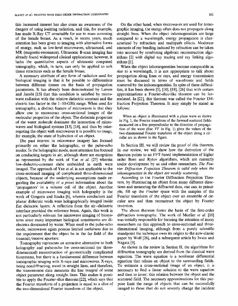
When an object is illuminated with a plane wave as shownin Fig. 1, the Fourier transform of the forward scattered fieldsmeasured on a line perpendicular to the direction of propaga-tion of the wave (line TT in Fig. 1) gives the values of thetwo-dimensional Fourier transform of the object along a cir-cular arc as shown in the figure.
In Section III, we will review the proof of this theorem.
In our review, we will show how the derivation of the
theorem points to an FFT-based implementation of higher
order Born and Rytov algorithms, which are currently
under development by us and other researchers. The Fou-
rier Diffraction Projection Theorem is valid only when the
inhomogeneities in the object are weakly scattering.
According to the Fourier Diffraction Projection Theo-
rem, by illuminating an object from many different direc-
tions and measuring the diffracted data, one can, in princi-
ple, fill up the Fourier space with the samples of tlheFourier transform of the object over an ensemble of cir-
cular arcs and then reconstruct the object by Fourier
inversion.
The above theorem ~forms the basis of the first-order
diffraction tomography. The work of Mueller et al. [18]
was initially responsible for focusing the attention of many
researchers on this approach to cross-sectional and three-
dimensional imaging, although from a purely scientific
standpoint the technique owes its origins to the now-classic
paper by Wolf [26], and a subsequent article by Iwata and
Nagata [9].
As shown in the review in Section II, the algorithms for
diffraction tomography are derived from the classical wave
equation. The wave equation is a nonlinear differential
equation that relates an object to the surrounding fields.To estimate a cross-sectional image of an object, it is
necessary to find a linear solution to the wave equation
and then to invert, this relation between the object and the
scattered field. The necessary approximations for this pur-
pose limit the range of objects that can be successfully
imaged to those that do not severely change the incident

862 IEEE TRANSACTIONS ON MICROWAVE THEORY AND TECHNIQUES, VOL. MTT-32, NO. 8, AUGUST 1984
....Meaaured forward . . . ...”””” ““...
eeattered tteld
.’””””””*4 ““”””..
W
....”-—Fourier transform
\ .—“.%,
\ Y ....
\\
\
=7P-\\\\\
space domain
Fig. 1. The Fourier diffraction theorem.
‘\\
\
frequeney domain
field or have a small refractive index gradient compared to
the surrounding media. In Section II, we will first review
the two most common approximations used, the first-order
Born and Rytov; and then in Section IV, we will show tlheeffects of these approximations on computer-simulated re-
constructions made from exact data.
These simulations will establish the first-order Born ap-
proximation to be valid for objects where the product of
the change in refractive index and the diameter is less than
0.35 A, and the first-order Rytov approximation for changes
in the refractive index of less than a few percent, with
essentially no constraint on the object size.
II. ASSUMPTIONS UNDERLYING FIRST-ORDER
DIFFRACTION TOMOGRAPHY
Diffraction tomography is based on a linear solution to
the wave equation. The wave equation relates an objectand the scattered field, and by linearizing it we can find art
estimate of a cross section of the object based on the
scattered field. The approximations used in the lineariza-
tion process are crucial to the success of diffraction tomogr-
aphy, and we will be careful to highlight the assumptions.
In a homogeneous medium, electromagnetic waves satisfy
a homogeneous wave equation of the form
(V’2+k&)4(?)=0 (:1)
where the wavenumber k. represents the spatial frequency
of the plane wave and is a function of the wavelength A, or
k. = 27r/X. It is easy to verify that a solution to (1) is given
by a plane wave
*(7) = eJZ’”7 (2)
where ~0 is the wave vector of the wave and satisfies the
relation l~o I = k.. For imaging, the interest is in an inho-
mogeneous medium, so the more general form of the wave
equation is written as
(V2+k(7)2)~(?)=0. (3)
For electromagnetic fields, if the effects of polarization are
ignored, k(?) can be considered to be a scalar function
representing the refractive index of the medium. We then
write
k(?) =kon(?) =ko[l+n~(?)] (4)
where k. now represents the average wavenumber of themedia, and n(?) is the refractive index as given by
‘(’)=i’TT (5)
The parameter na(?) represents the deviation from the
average of the refractive index. In general, it will be
assumed that the object of interest has finite support, so
n ~( 7) is zero outside the object. Here, we have used ~ and
c to represent the magnetic permeability and dielectric
constant and the subscript zero to indicate their average
values.
SLANEY et (d.: IMAGING WITH FIRST-ORDER DIFFRACTION TOMOGRAPHY 863
If the second-order terms in nd (i.e., no<< 1) are ignored point inhomogeneity, the Green’s function can be consid-
we find ered to represent the field resulting from a single point
(V2+k~)t(?)= -2k~n8(7)+(?)= -~(7)0(7) (6)
where 0(7) = 2k~n ~(?) is usually called the object func-
tion.
Note that (6) is a scalar wave propagation equation. Its
use implies that there is no depolarization as the electro-
magnetic wave propagates through the medium. It is known
[8] that the depolarization effects can be ignored only if the
wavelength is much smaller than the correlation size of the
inhomogeneities in the object. If this condition is not
satisfied, then, strictly speaking, the following vector wave
propagation equation must be used:
scatterer.
Since (11) represents the radiation from a two-dimen-
sional impulse source, the total radiation from all sources
on the right-hand side of (11) must be given by the
following superposition:
+~(7)=/G(H’) 0(7’) +(7)d7’. (15)
In general, it is impossible to solve (15) for the scattered
field, so approximations must be made. Two types of
approximations will be considered: the Born and the Rytov.
A. The Born Approximation
v2~(r)+k~n2~(?)–2v[1:.i =0 (7)
The Born approximation is the simpler of the two ap-
proaches. Consider the total field +(?) expressedas the. ... .
where ~ is the electric-field vector. A vector theory forsum of the incident field $.(7), and a small perturbation
diffraction tomography based on this equation has yet to+3(?) as in (9). The integral of ‘(15) is now written as
be developed.
In addition, *0(7), the incident field, is also defined as~,(?) =~G(7-7’)O(?’)~ O(?’)dr’
(v2+k;)~O(7) =0. (8)J
+ G(?–?’)0(7’)+~( ?’)dr’. (16)
Thus, tjO(7) represents the source field or the field present
without any object inhomogeneities. The total field may be If the scattered field ~$(?) is small compared to ~O(?), the
expressed as the sum of the incident field and the scattered effects of the second integral can be ignored to arrive at the
field approximation
+(?)=+.(?)++.(7) (9) ~,(7) =/G(7–?’)0(7’)~ 0(7’) dr’, (17)
with ~, satisfying the wave equation
(v’+k;)id~)=-+(~)o(~) (lo)
which is obtained by substituting (8) and (9) in (6). This
form of the wave equation will be used in the work to
follow.
The scalar Helmholtz equation (10) cannot be solved for
~,(?) directly, but a solution can be written in terms of a
Green’s function [16]. The Green’s function, which is a
solution of the differential equation
This constitutes the first-order Born approximation. For a
moment, let’s denote the scattered fields obtained in tlhismanner by @\l)(?). If one wished to compute $:’)(?), which
represents the second-order approximation to the scattered
fields, that could be accomplished by substituting *O i- ~i~)
for $0 in the right-hand side of (17), yielding
J~j2J(7) = G(7- 7’)0(7’)[1#0(7’)+ ~jl)(?’)] dr’. (18)
In general, we may write
(v2+k~)G(?l?’) =-?l(7-7’) (11)~~+’)(7) =~G(?-P)O(7’)[~0 (7’)+ ~~)(7)]dr’
is written in 3-space as
(1,9)#oRG(?l?’)=m
’12) for the higher (i+ l)th approximation to the scattered
with fields in terms of the ith solution, Since the science of
R= I?–?’l.reconstructing objects with higher order approximations is
(13) not fully developed, this particular point will not be pursued
In two dimensions, the solution of (11) is written in terms any further, and the first-order scattered fields will be
of a zero-order Hankel function of the first kind, and can represented by ~, (i.e., without the superscript).
be expressed as Note again that the first-order Born approximation is
valid only when the magnitude of the scattered fieldG(717’) = {Hjl)(kOR). (14)
+,(7)=+(7)-$.(7) (20)
In both cases, the Green’s function G(?l?’) is only a is smaller than that of the incident field tjO. If the object is
function of the difference 7 – ?’, so the argument of a cylinder of constant refractive index, it is possible to
the Green’s function will often be represented as simply express this condition as a function of the size of the object
G(? – ?’). Because the object function in (11) represents a (radius= a) and the refractive index. Let the incident wave

864 IEEE TRANSACTIONS ON MICROWAVE THEORY AND TECHNIQUES, VOL. MTr-32, NO. 8, AUGUST 1984
$.(?) ~e a plane wave propagating in the direction of thevector kO. For a large object, the field inside the object will
not be given by
~ (7)= 4’0~JeC,(7) + Ae~Z0”7 (21)
but instead will be a function of the change in refractive
index n ~. Along a ray through the center of the cylinder
and parallel to the direction of propagation of the incident
plane wave, the field inside the object becomes a slow (or
fast) version of the incident wave or
~object(~) = A.W+”8)ZOF (22)
Since the wave is propagating through the object, the
phase difference between the incident field and the field
inside the object is approximately equal to the integral of
the change in refractive index through the object. There-
fore, for a cylinder, the total phase shift through the object
is approximately
Phase Change = 47rn6 ~ (23)
where A is the wavelength of the incident wave. For the
first-order Born approximation to be valid, a necessary
condition is that the change in phase between the incident
field and the wave propagating through the object be less
than T. This condition can be expressed mathematically as
Anaa <—.
4(24)
B. The Rytov Approximation
The Rytov approximation is valid under slightly less
severe restrictions. It is derived by considering the total
field to be represented as [8]
~(?) = e$(~ (25)
and rewriting the wave equation (1) as
(V@)2+V2@ +k~=-2k~n8. (26)
Expressing the total phase @ as the sum of the incident
phase function $0 and the scattered complex phase ~, or
@(7) =@o(7)+ $.(?) (27)
where
*O(?) = e%(o (28)
we find that
( vqJ2+2vl#oT43 + ( V41J2+ V’+.
+V2@, +k:(l+2n8) =0. (29)
As in the Born approximation, it is possible to set the zero
perturbation equation equal to zero to find
2V~0.V+, + V2@~ = –(V@, )2–2k~n8. (30)
This equation is inhomogeneous and nonlinear, but can
be linearized by considering the following relation
V’($oo$) = v’+~”o$ +2V*O”V+S + +Ov’+,. (31)
Recalling that
+0= ~eJL?F (32)
we find
2+OV+0. V$. + +OV 20, = V’($O@, )+ k;toq$. (33)
This result can be substituted into (30) to find
(V2+k~)4@,= - 40[(V@,)2+2k&a]. (34)
As before, the solution to this differential equation can
again be expressed as an integral equation. This becomes
V@, = ~v,G(~– 0tO[(V%)2+2k;n~] dr’ (35)
where the Green’s function is given by (14).
Under the Rytov approximation, it is assumed that the
term in brackets in the above equation can be approxi-
mated by
(v’@, )2+2k~na = 2k&t8. (36)
When this is done, the first-order Rytov approximation to
the scattered phase O, becomes
Substituting the expression for ~, given in (17) yields
(38)
It is important to note that, in spite of the similarity of
the Born (17) and the Rytov (37) solutions, the approxima-
tions are quite different. As will be seen later, the Born
approximation produces a better estimate of the scattered
amplitude for large deviations in the refractive index for
objects small in size. On the other hand, the Rytov ap-
proximation gives a more accurate estimate of the scattered
phase for large-sized objects with small deviations in re-
fractive index.
When the object is small and the refractive index de-
viates only slightly from the surrounding media, it k possi-
ble to show that the Born and the Rytov approximations
produce the same results. Consider our definition of the
scattered phase in (25) and (27). Expanding the scattered
phase in the exponential with the Rytov solution to the
scattered field, it is seen
+(~) = e+o(i)+%(n = +o(~)eexp(-~zo ‘Jf’,(~. (39)
For very small ~,(?), the first exponential can be written
in terms of the power series expansion to find
t(7) =+o(~)[l +exp(–.jZ0.7) 4,(7) ]=+o(7)+ *f(7).
(40)
Thus, when the magnitude of the scattered field is very
small, the Rytov approximation simplifies to the Born
approximation.
The Rytov approximation is valid under a less restrictive
set of conditions than the Born approximation [4], [11]. In

SLANEY et al.: IMAGING WITH FIRST-06ER DIFFRACTION TOMOGRAPHY
deriving the Rytov approximation, the assumption was
made that
(V@,) 2+2k~n8 = 2k~na. (41)
Clearly this is true only when
n,>> (wd2k; “
(42)
This can be justified by observing that, to a first approxi-
mation, the scattered phase ~, is linearly dependent on n ~
[4]. If no is small, then
(Vq5S)2~n; (43)
will be even smaller, and, therefore, the first term in (41)
above can be safely ignored. Unlike the Born approxima-
tion, the size of the object is not a factor in the Rytov
approximation. The term VOJ is the change in the complex
scattered phase per unit distance, and by substituting k. =
27r/A, we find a necessary condition for the validity of the
Rytov approximation is
[1V4.A 2n8 >> —
2T “(44)
Therefore, in the Rytov approximation, it is the change in
scattered phase +, over one wavelength that is important
and not the total phase. Thus, because of the v operator,
the Rytov approximation is valid when the phase change
over a single wavelength is small.
III. INVERSION OF THE SCATTERED FIELDS
The Fourier Diffraction Theorem relates the Fourier
transform of the scattered field, the diffracted projection,
to the Fourier transform of the object along a circular arc.
While a number of researchers have derived this theory
[18], [5], [21], [12], we would like to propose a system
theoretic analysis of this result which is fundamental to
first-order diffraction tomography. This approach is super-
ior not only because it allows the scattering process,to be
visualized in the Fourier domain, but also because it points
to efficient FFT-based computer implementations of higher
order Born and Rytov algorithms currently under develop-
ment. Since it appears that the higher order algorithms will
be more computationally intensive, any savings in the
computing effort involved is potentially important.
Consider the effect of a single plane wave incident on an
object. The forward scattered field will be measured at a
receiver line as shown in Fig. 2. We will find an expression
for the field scattered by the object 0(?) by analyzing (17)
in the Fourier domain. We will use the plots of Fig. 3 toillustrate the transformations that take place.
The first-order Born equation for the scattered field (17)
can be considered as a convolution of the Green’s function
G(7) and the product of the object function 0(7) and the
incident field $.(?). First, we will define the following
865
Y
Measured field t
I
*
Incident plane wave
Fig. 2. A typical diffraction tomography experiment.
Fourier transform pairs:
where we have used the relationships
(46)
~ = (a, ~) and (a, /?) being the spatial frequencies along
the x and y directions, respectively.
The integral solution to the wave equation (17) can now
be written in terms of these Fourier transforms
J,(ii)= G(x){ b(A)*&(I)} (47)
where we have used ‘ *‘ to represent convolution. When
the illumination field ~0 consists of a single plane wave
with ~0 = ( kX, kY ) satisfying the following relationship
k;=k~+k; (49)’
its Fourier transform is given by
JO(I)=2778(X- ZI)). (50)
The delta function causes the ,convolution of (47) to be-
come a shift in the frequency domain as given by
o(x) *Jo(I) =2r6(i–&). (51)
866 IEEE TRANSACTIONS ON MICROWAVE THEORY AND TECHNIQUES, VOL. MT’E32, NO. 8, AUGUST 1984
(a)
Y
k
(b)
(c)
(d)
Aky
k
(e)
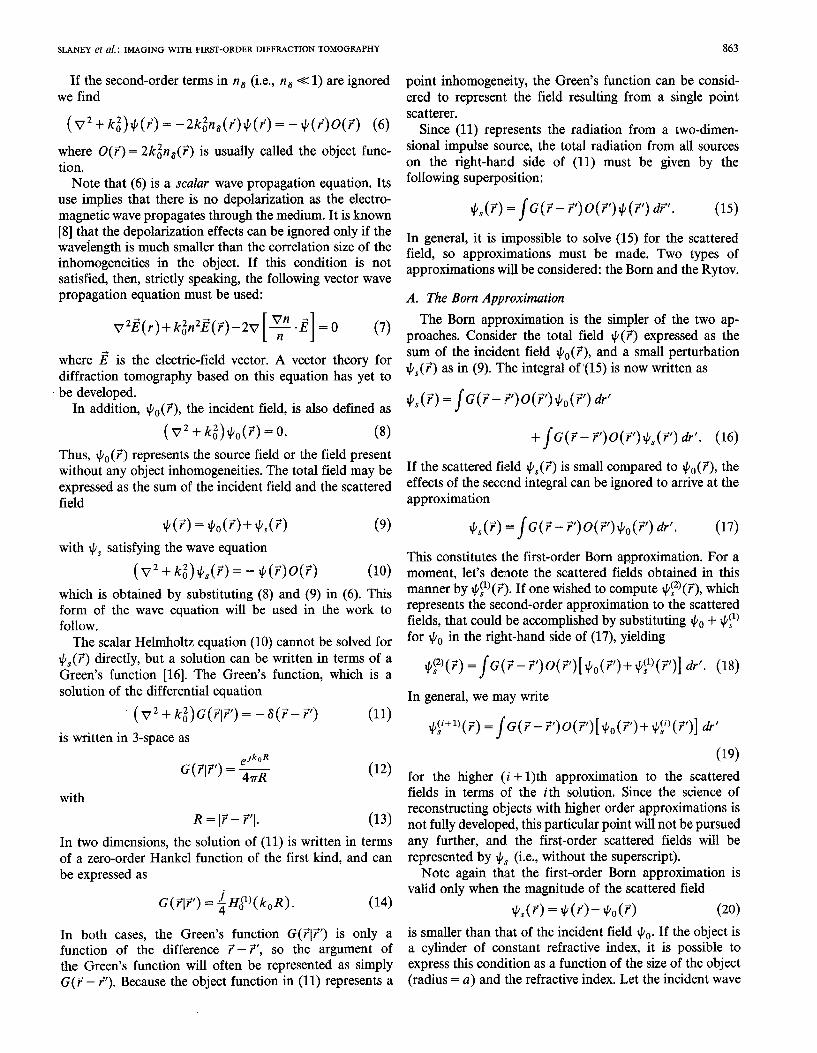
Fig. 3. Fourier spectrum representation of diffraction tomography ex-periment. (a) The object function, (b) the incident field, (c) the scatter-ing potential, (d) the Green’s function, and (e) the scattered field.
This convolution is illustrated in Fig. 3(a~–(c) for a plane
wave propagating with direction vector kO = (O, kO). Fig.
3(a) shows the Fourier transform of a single cylinder of
radius L!, and Fig. 3(b) is the Fourier transform of the
incident field. The resulting convolution in the frequency
domain (or multiplication in the space domain) is shown in
Fig. 3(c).
To find the Fourier transform of the Green’s function,
the Fourier transform of (11) is taken to find
(- A2+k:)~(~lF’)=- e-~l”r (52)
where A2 = a2 +/32. Rearranging terms, we see that
–“x.?’G(A17’)= :2’k3 (53)
has a singularity for all ~ such that
A2=a2+~2=k;. (54)
In the space domain, the two-dimensional Green’s func-
tion, (14), has a singularity at the origin so it is necessary to
approximate the function by using a two-dimensional aver-
age of the values near the singularity. An approximation to
G(A) is shown in Fig. 3(d).
The Fourier transform representation is misleading be-
cause it represents a point scatterer as both a sink and a
source of waves. A single plane wave propagating from left
to right can be considered in two different ways depending
on the point-of-view. From the left side of the scatterer, the
point scatterer represents a sink to the wave, while to the
right of the scatterer the wave is spreading from a source
point. Clearly, it is not possible for a scatterer to be both a
point source and sink and later, when the expression for
the scattered field is inverted, it will become necessary to
choose a solution that leads to outgoing waves only.
The effect of the convolution shown in (17) is a multipli-
cation in the frequency domain of the shifted object func-
tion, (51), and the Green’s function, (53), evaluated at7’= O. The scattered field is written as
(55)
This result is shown in Fig. 3(e) for a plane wave propagat-
ing along the y axis. Since the largest frequency domain
components of the Green’s function satisfy (l), the Fourier
transform of the scattered field is dominated by a shifted
and sampled version of the object’s Fourier transform.
We will now derive an expression for the field at the
receiver line. For simplicity, it will be assumed that the
incident field is propagating along the positive y axis or
k. = (O, ko). The scattered field along the receiver line
(x, y =1) is simply the inverse Fourier transform of the
field in (55). This is written as
which, using (55), can be expressed as
(57)
We will carry out the integration with respect to ~. For a
given a, the integral has a singularity at
&2= ~{k; - a2 . (58)
Using contour integration, we can close the integration
path at infinity and evaluate the integral with respect to/3

SLANEY et a[.: IMAGING WITH FIRST-ORDER IXFFRACTION TOMOGRAPHY 867
Fig. 4. Path of integration to calculate two-dimensionafscatteredfields.
along the path shown in Fig. 4 to find
IObject’sky
I Object’s
k.
*$(x,y=/) =Jrl(a; l)eJ”’da+Jr2(~;l)eJ”’d~I
Fig. 5. The transmitted and reflected fields provide information abouttwo different arcsin the object’sFourier domain.
(59)
where receiver line at y = 1 greater than the object. This can be
o(a,~~– ‘0) ~jp/considered transmission tomography. Conversely, the
rl = (60) dashed line indicates the locus of solutions for y= 1 less
j2{~ than the object or the reflection tomography case.
Straight-ray (i.e., X-ray) tomography is based on the
Fourier Slice Theorem [10], [22]and
O(rx, -/k;-a* – ‘0)e-j-lr2 = (61)– j2{~
Examining the above pair of equations, it is seen that 1’1
represents the solution in terms of plane waves traveling
along the positive y axis while 172represents plane waves
traveling in the – y direction. In both cases, as a ranges
from – /c. to ko, r represents the Fourier transform of the
object along a semi-circular arc.
Since we are interested in the forward traveling waves,
only the plane waves represented by the rl solution are
valid, and thus the scattered field beeomes
+.(x, y= 1) =Jrl(a; i)ejaxda, 1> object (62)
where we have chosen the value of the square root to lead
only to outgoing waves.
Taking the Fourier transform of both sides of (62), we
find that
J(+, x,y=l)e-’axdx =f’(a,l). (63)
But since r(x, 1) is equal to a phase-shifted version of the
object function, the Fourier transform of the scattered field
along the line y = 1 is related to the Fourier transform of
the object along a circular arc, The use of the contour
integration is further justified by noting that only those
waves that satisfy the relationship
a2+~2=k; (64)
will be propagated, and thus it is safe to ignore all waves
not on the ko-circle.
This result is diagramed in Fig, 5. The circular arc
represents the locus of all points (a, /3) such that /3=
+ f=. The solid line shows the outgoing waves for a
The Fourier transform of a parallel projection of an imagef(x, y) taken at an angle O gives a slice of the two-dimen-sional transform, F( w], W2) subtending an angle O with theriq axis.
This is diagramed in Fig. 6.
Equation (63) leads us to a similar result for diffraction
tomography. Recall that a and /3 in (63) are related by
/! I=/p. (65)
Thus, f’(a), the Fourier transform of the received field, is
proportional to O(a, P – ko), the Fourier transform of theobject along a circular arc. This result has been called the
Fourier Diffraction Projection Theorem [21] and is dia-
gramed in Fig. 1,
We have derived an expression, (63), that relates the
scattering distribution of an objeet to the field received at a
line. Within the diffraction limit, it is possible to invert this
relation to estimate the object scattering distribution based
on the received field.
A number of experimental procedures have been pro-
posed to collect the data required to reconstruct the com-
plete object. A single incident plane wave generates infor-
mation along an arc in the object’s Fourier domain, and by
rotating the object [18], varying the frequency of the il-
luminating field [12], or by synthesizing an aperture [19], it
is possible to fill up the Fourier space.
In addition, there are two types of algorithms that can
be used to estimate the object. As proposed by Soumekh
et al. [23], they can be described as interpolation in either
the frequency or space domain. A comparison of these two
methods has been published in [21].
The Fourier Diffraction Projection Theorem establishes
a connection between the diffracted projections and an
estimate of the object’s Fourier transform along circular

868 IEEE TRANSACTIONS ON MICROWAVE THEORY AND TECHNIQUES, VOL. Mm-32, NO.8, AUGUST1984
..................................
\
W2
@A
B
+ w,
“.. ...
space domain frequency domain
Fig. 6. The Fourier slicetheorem.
arcs. The fact that the frequency domain samples are
available over circular arcs, whereas, for fast Fourier inver-
sion, it is desired to have samples over a rectangular lattice,
is a source of computational difficulty with a direct Fourier
inversion technique. Mueller et al. [17] have shown that by
using nearest neighbor interpolation, it is possible to ade-
quately map the data onto a rectangular grid and then use
an FFT algorithm to invert the data. More sophisticated
approaches are discussed in [21].
An interpolation procedure in the space domain was first
proposed by A. J. Devaney [5]. This approach is similar to
the backprojection algorithm [10] that made X-ray tomog-
raphy successful, but since a propagation filter is applied
to the projection data as it is smeared over the image plane,
it has been called filtered-backpropagation. Since the prop-
agation filter is depth-dependent, this approach is com-
putationally more expensive than the frequency domain
interpolation approach, It has been shown [21] that recon-
structed images with bilinear interpolation are comparable
in quality to those produced by filtered-backpropagation.
IV. DISTORTIONS INTRODUCED BY
FIRST-ORDER ALGORITHMS
Several hundred computer simulations were performed
to study the fundamental limitations of first-order diffrac-
tion tomography. In diffraction tomography, there are
different approximations involved in the forward and in-
verse directions. In the forward process, it is necessary to
assume that the object is weakly scattering so that either
the Born or the Rytov approximations can be used. Once
we arrive at an expression for the scattered field, it is
necessary to not only measure the scattered fields but then
numerically implement the inversion process.
The mathematical and experimental efiects limit the
reconstruction in different ways. The most severe mathe-
matical limitations are imposed by the Born and the Rytov
approximations. These approximations are fundamental to
the reconstruction process and limit the range of objects
that can be examined. On the other hand, the experimental
limitations are caused because it is only possible to collect
a finite amount of data. Up to the limit in resolution
caused by evanescent waves, it is possible to improve a
reconstruction by collecting more data.
By carefully setting up the simulations, it is possible to
separate the effects of these errors. To study the effects of
the Born and the Rytov approximations, it is necessary to
calculate (or even measure) the exact fields and then make
use of the best possible (most exact) reconstruction for-
mulas available. The difference between the reconstruction
and the actual object can then be used as a measure of the
quality of the approximations.
These simulations are similar to a study performed by
Azimi and Kak. In [3], the effects of multiple scattering on
first-order diffraction tomography algorithms were dis-
cussed for objects consisting of multiple cylinders, It was
concluded that even when object inhomogeneities are as
small as 5 percent of the background, multiple scattering
can introduce severe distortions in first-order reconstruc-
tions.
A. Qualitative Analysis
The exact field for the scattered field from a cylinder as
shown by Weeks [25] was calculated for cylinders of vari-
ous sizes and refractive index. In the simulations thatfollow, a single plane wave was incident on the cylinder,
and the scattered field was calculated along a line at a
distance of 100 wavelengths from the origin.
At the receiver line, the received wave was measured at
512 points spaced at 1/2 wavelength intervals. In all cases,
the rotational symmetry of a single cylinder at the origin
was used to reduce the computation time of the simula-
tions.
The simulations were performed for refractive indices
that ranged from O.1-percent change (refractive index of
1.001) to a 20-percent change (refractive index of 1.2), For
each refractive index, cylinders of size 1, 2, 4, and 10

SLANEY et a[.: IMAGING WITH FIRST-ORDER DIFFRACTION TOMOGRAPHY
1.001 1.01 1.,10 1.20
1A
21
4X.
1OA
Fig. 7. Reconstructionsusing the Born approximation for cylinders ofradius 1, 2, 4, and 10A, aud refractive indices of 1.001,1.01, 1.10, and1.20.
wavelengths were reconstructed. This gave a range of phase
changes across the cylinder (see (23) above) from 0.0047r to
87r. The resulting reconstructions using the Born approxi-
mation are shown in Fig. 7,
Clearly, all the cylinders of refractive index 1.001 in Fig.
7 were perfectly reconstructed. As (24) predicts, the results
get worse as the product of refractive index and radius gets
larger. The largest refractive index that was successfully
reconstructed was for the cylinder in Fig. 7 of radius 1
wavelength and a refractive index that differed by 20
percent from the surrounding medium.
While it is hard to evaluate the two-dimensional recon-
structions, it is certainly reasonable to conclude that only
cylinders where the phase change across the object was less
than or equal to 0.877 were adequately reconstructed. In
general, the reconstruction for each cylinder where thephase change across the cylinder was greater than n shows
severe artifacts near the center. This limitation in the phase
change across the cylinder is consistent with the condition
expressed in (24) above.
A similar set of simulations was also done for the Rytov
approximation, and is shown in Fig. 8. In this case, the
reconstructions were performed for cylinders of radius 1, 2,
40, and 100 A, and refractive indices of 1.001, 1,01, 1.05,
and 1.10. Because of the large variation in cylinder sizes,
al reconstructions were performed so that the estimated
object filled half of the reconstruction matrix. While the
error in the reconstructions does increase for larger cylin-
ders and higher refractive indices, it is possible to success-
fully reconstruct larger objects with the Rytov approxima-
tion.
B. Qualitative Comparison of the Born and
Rytov Approximation
Reconstructions using exact scattered data show the
similarity of the Born and Rytov approximations for. small
objects with small changes in the refractive index. For. a
cylinder of radius 1 wavelength and a refractive index that
differs by 1 percent from the surrounding medium, the
resulting reconstructions are shown in Fig. 9. In both cases,
869
I.cml 1.01 I .06 1.10
Ii
2!.
40i
Iooh
Fig. 8. Reconstructionsusing the Rytov approximation for cylinders ofradius 1,2,40, and 100A, and refractive indicesof 1.001,1.01,1.05, anc~1.10.
A Rytov
Fig. 9. Born and Rytov reconstructionsof a 1 cylinder of 1A radius and1.01refractive index.
the reconstructions are clean and the magnitude of the
reconstructed change in refractive index is close, to the
simulated object.
On the other hand, the reconstructions of objects that
are large or have a refractive index that differ by a large
factor from one illustrate the differences between the Born
and the Rytov approximations. Fig. 10 shows a simulated
reconstruction for an object of radius 1 and refractive
index of 1.20. In this region, the Born approximation i;s
superior to the Rytov.
According to Chemov [4] and Keller [11], the Rytov
approximation should be much superior to the Born for
objects much larger than a wavelength, Reconstructions

870 IEEE TRANSACTIONS ON MICROWAVE THEORY AND TECHNIQUES, VOL MTT-32,NO.8, AUGUST 1984
I’!lBorn
Fig. 10. Reconstructions of a radius 1A cylinder and refractive index1.20showingthe advantageof the Born over the Rytov.
Fig. 11. Reconstructions of a radius 40A cylinder and refractive index1.01showing the advantageof Rytov over the Born.
were done based on the exact scattered wave from a
cylinder of radius 40 wavelengths and a refractive index
that differed by 1 percent from the surrounding medium.
The reconstructed refractive index is shown in Fig. 11.
While the Born approximation has provided a good esti-
mate of the size of the object, the reconstruction near the
center is clearly not accurate.
The results in Figs. 10 and 11 are consistent with the
regions of validity of the Born and Rytov approximations.
The Born approximation is sensitive to the total phase shift
in the object. Thus, in the reconstruction of Fig. 10, the
Born approximation has done a good job of representing
the step change in refractive index, but as the incident field
undergoes a phase shift through the object, the reconstruc-
tion becomes poor. On the other hand, the Rytov ap-
proximation is sensitive to the change in refractive index.
Thus, the Rytov reconstruction is accurate near the center
of the object but provides a very poor reconstruction near
the boundary of the object.
C. Quantitative Studies
In addition to the qualitative studies, a quantitative
study of the error in the Born and Rytov reconstructions
was also performed. As a measure of error, we used the
relative mean squared error in the reconstruction of the
object function integrated over the entire plane. If the
actual object function is 0(7) and the reconstructed object
function is 0’(7), then the relative Mean Squared Error
(MSE) is
To study
MSE =j“~[O(~)-O’(~)]2dF
(66)
jj[O(7)]2d7 “
the quantitative difference between the Born
and the Rytov approximations, several hundred simulated
reconstructions were performed. For each simulation, the
exact scattered field was calculated for a single cylinder
with an arbitrary radius and refractive index. The recon-
structions were divided into two sets to highlight the dif-
ference between the Born and the Rytov approximations.
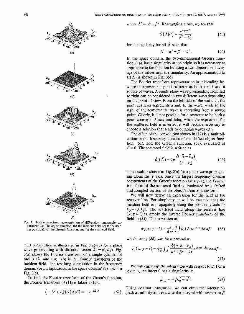
The plots of Fig. 12 present a summary of the mean
squared error for cylinders of 1, 2, and 3 A in radius and
twenty refractive indices between 1,01 and 1.20. In each
case, the error for the Born approximation is shown as a
solid line, while the error for the Rytov approximation is
shown as a dashed line. The exact scattered fields were
calculated at 512 receiver points along a receiver line 10X
from the center of the cylinder.
Only for the 1A cylinders is the relative mean squared
error for the Born approximation always lower than the
Rytov. It is interesting to note that, while the Rytov
approximation shows a steadily increasing error with higher
refractive indices, the error in the Born reconstruction is
relatively constant until a threshold is reached. For the 2A
and the 3A cylinder, this breakpoint occurs at a phase shift
of 0.6 and 0.77r. Thus, a criteria for the validity of the Born
approximation is that the product of the radius of the
cylinder in wavelengths and the change in refractive index
must be less than 0.175.
Fig. 13 presents a summary of the relative mean squared
errors for cylinders with refractive indices of 1.01, 1.02,
and 1.03 and for forty radii between 1 and 40 L Because
the size of the cylinders varied by a factor of forty, the
simulation parameters were adjusted accordingly. For a
cylinder of radius R, the scattered field was calculated for
512 receivers along a line 2R from the center of the
cylinder and spaced at l/16R intervals.
SLANEY et d: IMAGINGWITHFIRST-ORDERDIFFRACTIONTOMOGRAPHY 871
t900000-
.emaoo-
.750000-1:
~ .6.??000- ;~ :
* SYooooo-.z.# .’JEaoo- )’
,’,,
.?50000- /’,>’
,/-,1.3000- /.
.-
. .-.
.,..’
..----
~..-.,
/ .--.-”~-.
-~..
.000 1.0s375 t.05750 1.081?51,105001!12675 t.tY2al tlt76?5 I.aooo
Refracctue lnde%
2.4
0.00000 ,1.010001.03375 I!05750 t,oatn 1.10540 1.126r5 1.tY.2Yo1.176.?51,,?0000
Refract~ve Index
t .00000
emmo
]
a750000
& ,6E5000-
~ /
$ ,s00000-. /’
; ,. ,$ ,37$000- /’,
,,
.2%000- ,’/’
.’..’
.125000- .,-.
1.01
t .00000-
J.emoo-.?KiOoo-
& .6.zmOO-
;
$ .%0000-.$; .’37300-
.s50000-
0 tc?moo
L___—.-- ---------- -----------0,00000+t t
6 (1 16 .?1 a 30 35 w
Cyl mder Radtus
t.00000-
.8?5000- I.mooo -
~ .6?%00-
&
$ @Yooooo-.z# .%5000-
.mooo -
,t.?woo----
1.02
--.------------------ “------
1.00000
;WYOoo
0.00000-1 #16 tt t6 a 25 30 Ss WI
,
0,000004t.01000 1.03975 1.0S7?41.06!25 t.10%001.1?S75!.1SS54 1.176251..20000
Refract Lve index
$ IYooooo
II
; .3?5000
.aaooo
0.00000
Cyl mder Rad~us
6 11 16 21 .?5 % 35 w
Cyl lnder Rad t us
Fig. 12. The relative mean squarederror of the Born (solid lines) aud Fig. 13. The relative mean squarederror of the Born (solid lines) andRytov (dashed lines) approximations as a function of refractive index Rytov (dashed fines) approximations as a function of radius for cylin-for cylinders of radius 1, 2, and 3A. ders of refractive index 1.01,1.02, mid 1.03.

872 IEEE TRANSACTIONS ON MICROWAVE THEORY AND TECHNIQUES, VOL. MTT-32, NO. 8, AUGUST1984
In each of the simulations, the Born approximation is
only slightly better than the Rytov approximation until the
Born approximation crosses its threshold with a phase shift
of 0.7n-. Because the error in the Rytov approximation is
relatively flat, it is clearly superior for large object and
small refractive indices. Using simulated data and the
Rytov approximation, we have successfully reconstructed
objects as large as 2000A in radius.
D. Phase Error in the Born Approximation
The importance of the total phase shift of the incident
field under the Born approximation was confirmed by
considering the unwrapped phase of the reconstruction. Ho
and Carter [7] proposed that the Born approximation
actually reconstructs an estimate of the object function
multiplied by the total field.
Recall the integral equation (15) which forms the basis
of our reconstruction process:
~,(?) =~O(?’)+0(7’)G( 7-7’)d~. (15)
An alternative to the Born approximation is to define
(67)
and to substitute this modified object function 0’(7) for
0(7) in the integral of (17) above to find
+,(7) =~0’(7’)+o(7’)G( H’)dF’. (17)
Since $.(7) and G(? – ?’) are known exactly, for a single
incident plane wave, the relationship between the scattered
field and 0’(7) is exact. In practice, a tomographic image
is formed using the information from multiple incident
plane waves, and thus the reconstruction of 0’(?) can only
provide approximate information about the failure of the
Born approximation under large phase changes.
It is the relation between our exact estimate for 0’(?)
and the actual object function 0(?) that we would like to
investigate. Under the first Born approximation, we have
assumed that
+o(~)>>+.(~) (68)
and thus to a good approximation
+(7)=+.(7)! (69)
Here
(70)
and thus our reconstruction procedure yields a good esti-
mate of the object.
For objects that do not satisfy the Born approximation,
part of the reconstruction error shows up as a phase shift.
In (23), we estimated that a ray passing through the center
of a homogeneous cylinder undergoes a phase shift of
4i7n8aPhase Change = ~. (23)
Phase of Reconstruction (Not to Scale)
Refractive Index 1.01 Refractive Index 1.03
Refractive Index 1.06 Refractive Index 1.07
Refractive Index 1.10
Fig. 14.
Refractive Index 1.20
Refractive Index 1.16
Totaf unwrapped phase of the Born reconstnrction for a 10Acylinder with a refractive index between 1.01 and 1.20.
Thus, to a first approximation, the reconstruction of 0’(7)
is related to the actual object function 0(?) by
0’(?) = o(~) elz~(~j~/~) (71)
where d represents the distance to the boundary of the
object.
This approximate relationship was studied through a
number of simulations. Fig. 14 shows the phase of the
reconstruction of a cylinder with radius 10A and refractive
index that varied between 1.01 and 1.20. The phase of the
reconstruction was unwrapped with a phase unwrapping
algorithm proposed by Tribolet [24] and extended to two
dimensions by O’Conner and Huang [20].
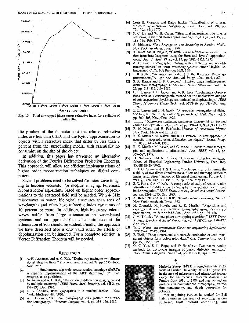
The total phase error at the center of a 10X cylinder is
shown in Fig. 15. While the total phase error does increasewith refractive index at large refractive indices, it is ap -
parent that a more complete theory is needed to estimate
the object function more accurately,
V. CONCLUSIONS
By carefully designing a simulation procedure, we have
isolated the effects of the first-order Born and Rytov
approximations in diffraction imaging. While both proce-
dures can produce excellent reconstructions for small ob-
jects with small refractive index changes, they both quickly
break down when their assumptions are violated. The
assumptions limit the Born approximation to objects where
SIANEY d a[.: IMAGING WITH FIRST-OROER DIFFRACTION TOMOGRAPHY
23. ?065-
zO.e20a -
t7.9w6 -.wc
~ ‘=’07”v
~ 1?.s19?s-
Lhal 9.mwtt -Wm
E6. WtbO -
3,55759 -
.-~1,01000 1,0337Y 1.05750 1.0s1?S 1.10500 1.1.?S7S1.t5?S0 1.17625 t.?QOOO
l?efrac~lve Index
Fig. 15. Totaf unwrapped phase versus refractive index for a cylinder ofradius 10A.
the product of the diameter and the relative refractive
index are less than 0.35A and the Rytov approximation to
objects with a refractive index that differ by less than 2
percent from the surrounding media, with essentially no
constraint on the size of the object.
In addition, this paper has presented an alternative
derivation of the Fourier Diffraction Projection Theorem.
This approach will allow for efficient implementations of
higher order reconstruction techniques on digital com-
puters.
Several problems need to be solved for microwave imag-
ing to beeome successful for medical imaging. Foremost,
reconstruction algorithms based on higher order approxi-
mations to the scattered field will be needed. With 4-GHz
microwaves in water, biological structures span tens of
wavelengths and often have refractive index variations of
10 percent or more. In addition, high-frequency microw-
aves suffer from large attenuation in water-based
systems, and an approach that takes into account the
attenuation effects should be studied. Finally, the approach
we have described here is only valid when the effects of
depolarization can be ignored. For a complete solution, a
Vector Diffraction Theorem will be needed.
REFERENCES
[1] A. H. Andersen and A. C. Kak, “ Digitaf ray tracing in two-dimen-sionaf refractive fields< J. Acoust. Sot. Am., vol. 72, pp. 1593–1606,NOV. 1982.
[2] _, “Simultaneous algebraic reconstruction technique (SAR~:A superior implementation of the ART algorithm; UltrasonicImaging, to be published.
[3] M. Azimi and A. C. Kak, “ Distortion in diffraction imaging causedby multiple scattering IEEE Trans. Med. Imaging, vol. MI-2, pp.176-195, Dec. 1983.
[4] L. A. Chemov, Wave Propagation in a Random Medium. NewYork: McGraw-Hill, 1960.
[5] A. J. Devaney, “A filtered backpropogation algorithm for diffrac-tion tomography: Ultrasonic Imaging, vol. 4, pp. 336–350,1982.
[6]
[7]
[8]
[9]
[10]
[11]
[12]
[13]
[14]
[15]
[16]
[17]
[18]
[19]
[20]
[21]
[22]
[23]
[24]
[25]
[26]
[27]
873
Loris B. Greg,oris and Keigo Iizuka, “Visualization of intenmfstructure by &crowave holography;’ Proc. IEEE, vol. 594, pp.791-792, Mav 1970.P. C. Ho and W. H. Carter, “ Strncturaf measurement by inversescattering in the first Born approximation,” Appl. Opt., vol. 15, pp.313-314. Feb. 1976.A. M&m, Wave Propagation and Scattering in Random Media.
New York: Academic Press, 1978.K. Iwata and R. Nagata, “Calculation of refractive index distrib-ution from interferograms using the Born and Rytov’s approxima-tions; Jap. J. Appl. Phys.j vol. 14, pp. 1921-1927, 1975.A. C. Kak, “Tomographic imaging with diffracting and non-dif-fracting sources,” in Array Processing Systems, Simon Haykin, Fkf.Englewood Cliffs, NJ: Prentice Hall, 1984.J. B. Keller, “Accuracy and validity of the Born and Rytov ap-proximations; J. Opt. Sot. Am., vol. 59, pp. 1003-1004, 1969.S. K, Kenue and J, F. Greenleaf, “Limited angle muhifrequencydiffraction tomogral.rhv,” IEEE Trans. Sonics Ultrasonics, vol. SU-29, pp. 213-217,-Juiy ~982.L. E. Larsen, J. H. Jacobi, and A. K. Kreyj “Preliminary obser-va-tions with an electromagneticmethod for the noninvasive analysisof cell suspensionphysiology and induced pathophysiology~ IEEETrans. Microwave Thepry Tech., vol. MTT-26, pp. 581-595, Aug.1978.L. E. Larsen and J. H. Jacobi, “Microwave interrogation of dielec-tric targets: Part 1: By scattering parameters,” Med. Phys., vol. 5,
PP. 500-508, Nov./Dee. 1978.“Microwave scattering parameter imagery of an isolated
c=e’kidney~ Med. Phys., vol. 6, pp. 394-403, Sept./Ott. 1979.P. M. Morse and H. Feshbach, Methods of Theoretical Physics.New York: McGraw-Hill, 1953.R. K. Mueller, M. Kaveh, and R. D. Iversen, “A new approach. toacoustic tomography using diffraction techniques,” A coast, Imag.,
vol. 8, pp. 615–628, 1980.R. K. Mueller, M. Kaveh, and G. Wade, “Reconstructive tomog~a-phy and applications to ultrasonic” Proc. IEEE, vol. 67, pp.567-587, 1979.D. Nahamoo and A. C. K&, “Ultrasonic diffraction imagitr,g,”School of Ele@caf Engineering, Purdue University, Tech. Rep.TR-EE-82-20, 1982.B. T. O’Conrior and T. S. Huang, “Techniques for determining thestability of two-dimensionaf recursive filters and their application toimage restoration,” School of Electrical Engineering, Purdue Uni-versity, Tech. Rep. TR-EE-78-18, pp. 6–24, May 1978.S. X. Pan and A. C. Kak, “A computational study of reconstinctionalgorithms for diffraction tomography: Interpolation vs. filteredbackpropagation~ IEEE Trans. A court., Speech and Signal Process-
ing, pp. 1262–1275, Oct. 1983.A. Rosenfeld and A. C. Kak, Digital Picture Processing, 2nd ed.New York: Academic Press, 1982.M. Soumekh, M. Kaveh, and R. K. Mueller, “Algorithms andexperimental results in acoustic tomography using Rytov’s ap-proximation,” in ICASSP 83 Proc., Apr. 1983, pp. 135-138.J. M. Tribolet, “A new phase unwrapping algorithm< IEEE Trans.Acoo.rt., Speech and Signal Processing, vol. ASSP-25, pp. 170-1.77,Apr. 1977.W. L. Weeks, Electromagnetic Theory for Engineering Applications.New York: Wiley, 1964.E. Wolf, “ ‘rhree-dimensional structure determination of semi-trans-parent objects form holographic data; Opt. Communicant., vol. 1,pp. 153-156,1969.0. C. Yue, E. L. Rope, and G. Tricoles, “Two reconstructionmethods for microwave imaging of buried dielectric anomalie,”IEEE Trans. Computers, vol. C-24, pp. 381-390, Apr. 1975.
*
Malcolm Slaney (M83) is completing his, Ph.D.work at Purdue University, West Lafayette, IN,in the area of microwave and ultrasound tomog-raphy. He has been a Research Associate atPurdue from 1981 to 1984 and has worked onproblems in computerized tomography, diffrac-tion tomography, and depth perception forrobotics.
Prior to joining Purdue, he worked for BellLaboratories in the areas of switching systemssoftware, fault tolerant computing, and

874 IEEE TRANSACTIONS ON MICROWAVE THEORY AND TECHNIQUES, vOL. MTr-32$ NO, 8, AUGUST 1984
high-speed digital networks. Over the past few years, he afso has consultedwith several companies in the areas of digitaf control systems, X-raytomography, and doppler ultrasound.
Mr. Slaney is a member of ACM and Eta Kappa Nu.
*
Avinash C. Kak (M71) is currently a Professor ofElectrical Enzineenng at Purdue University, WestLafayette, Ifi. His c~rrent research interests arein computed imaging, image processing, andartificia3 intelligence. He has coauthored Digital
Picture Processing, vols. 1 and 2 (New York:Academic), a second edition of which was pub-lished in 1983. He is an Associate Editor ofComputer Vision, Graphics and Image Processing(New York: Academic), and Ultrasonic Imaging
(New York: Academic). He was also a Guest
Editor of the February 1981 SDeciaf Issue on Commrted Imazinz of theIEEE TRANSACTIONSON BIO~DICAL ENGINEEIUN& During &e last tenyears, he has consulted in the areas of computed imaging for manyindustrial and governmental organizations.
*
Lawrence E. Larsen (M81-SM82) attended andreceived the M.D. degree magna cum laude fromthe University of Colorado, Fort Collins, in 1968.He was awarded an NIH postdoctoral fellowshipin biophysics at UCLA for the period 1968–1970.
He then served in the United States Army as aResearch Physiologist in the Department of i’@crowave Research at the Wafter Reed Army In-stitute of Research during 1970–1973. From 1973to 1975, he accepted a faculty appointment in theRadiology Department at the Baylor College of
Medicine in Houston, TX, wh=~e he- taught physiology- and computersciences. In 1975, he returned to the Walter Reed Army Institute ofResearch as the Associate Chief of Microwave Research. He was ap-pointed the Department Chief in 1977 and presently serves in that rolewith the rank of Colonel, Medical Corps. He holds several patents.
Hyperthermia and Inhomogeneous TissueEffects Using an Annular Phased Array
PAUL F. TURNER
Abstract —A regional hypcrthermia Annular Phased Array (APA) appli-
cator is described, and examples of its various heating patterns, obtained by
scanning the electric fields with a smafl E-field sensor, are illustrated. Also
shown are the effects of different frequencies of an elliptical phantom
cylinder having a l-cm-thick artificial fat wall and the generaf dimensions
of the humau trunk. These studies show the APA’s ability to achieve
uniform heating at lower frequencies (below 70 MHz) or to focus centraf
heating at moderately higher frequencies (above 70 MHz). The influence
of human anatomical contours in afterirrg heating patterns is discussed
using results obtained with a female mannequin having a thin latex shell
filled with tissue-equivalent phantom. Field perturbations caused by intem-
afly embedded low-dielectric structures are presented, showing the localized
effects of smafl objects whose surfaces are perpendicular to the electric
field.
I. INTRODUCTION
E LECTROMAGNETIC (EM) hyperthermia has been
clinically tested, for the most part, with superficial
tumors in which the response is easily measured, Results
obtained in these clinical trials corroborate findings from
Manuscript received October 12, 1983; revised March 8, 1984.The author is with BSD Medical Corporation, 420 Chipeta Way, Suite
220, Salt Lake City, UT 84108.
earlier in vivo and in vitro experiments that show this
technique to be capable of selectively treating cancerous
tumors. Much of the real potential of hyperthermia, how-
ever, lies in its ability to treat deep-seated localized tumors
for which surgical removal is not a feasible solution. Such
tumors have consistently presented one of the most dif-
ficult challenges facing both oncologists and technical re-
searchers.
In response to this need, BSD Medical Corporation has
developed an EM Annular Phased Array, or APA (patent
pending), shown in Fig. 1, which has undergone testingsince 1979 and which, during that time, has been shown to
be capable of transmitting heating power directly to central
body tissues [1]. The interaction of the human body and
the EM field generated by the APA has been studied with
phantom models [2], anesthetized laboratory animals [1],
[3], and terminally ill human cancer patients [4], [5], Re-
sults obtained in these trials show that deep regional
hyperthermia is not only possible, but effective in control-
ling solid tumors in the center of the body. (Actual clinical
application of this method is still restricted, primarily
0018-9480/84/0800-0874$01.00 01984 IEEE