Likelihood Methods in EcologyJune 2nd – 13th, 2008

New York, NY

Instructors:Charles Canham and María Uriarte

Teaching AssistantCharles Yackulic

Daily Schedule

Morning- 8:30 – 10:00 Lecture

- 10:00 – 10:30 Break

- 10:30 – 12:30 Lab Lunch 12:30 – 2:00 Afternoon

- 2:00 – 3:00 Discussion

- 3:00 – 3:30 Break

- 3:30 – 5:30 Individual Projects

Syllabus

Introduction Know your data Formulate models Estimate parameters Evaluate individual models Compare alternate models Inference from models Advanced topics

Likelihood is much more than a statistical method...(it can completely change the way you ask and answer questions…)

Introduction to Likelihood and Model Comparison

Lecture 1

Day 1 Lecture...

Probability and probability density functions

Statistical inference Classical “frequentist” statistics

- Limitations and mental gyrations... The “likelihood” alternative

- Basic principles and definitions Model comparison as a generalization of

hypothesis testing A simple example: The maximum

likelihood approach to linear regression

A simple definition of probability for discrete events...

“...the ratio of the number of events of type A to the total number of all possible events (outcomes)...”

The enumeration of all possible outcomes is called the sample space (S).     If there are n possible outcomes in a sample space, S, and m of those are favorable for event A, then the probability of event, A is given as    

P{A} = m/n

Probability defined more generally...

Consider an outcome X from some process that has a set of possible outcomes S:

- If X and S are discrete, then P{X} = X/S

- If X is continuous, then the probability has to be defined in the limit:

b

a

ba dxxgxXxP )(}{

Where g(x) is a probability density function (PDF)

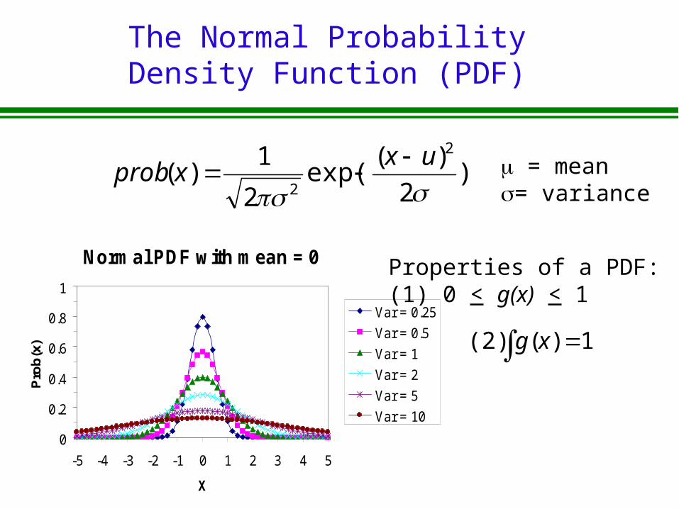
The Normal Probability Density Function (PDF)

Normal PDF with mean = 0

0

0.2

0.4

0.6

0.8

1

-5 -4 -3 -2 -1 0 1 2 3 4 5

X

Pro

b(x

)

Var = 0.25

Var = 0.5

Var = 1

Var = 2

Var = 5

Var = 10

)2

)(exp(

2

1)(

2

2 ux

xprob

= mean= variance

Properties of a PDF:(1) 0 < g(x) < 1

1)( (2) xg

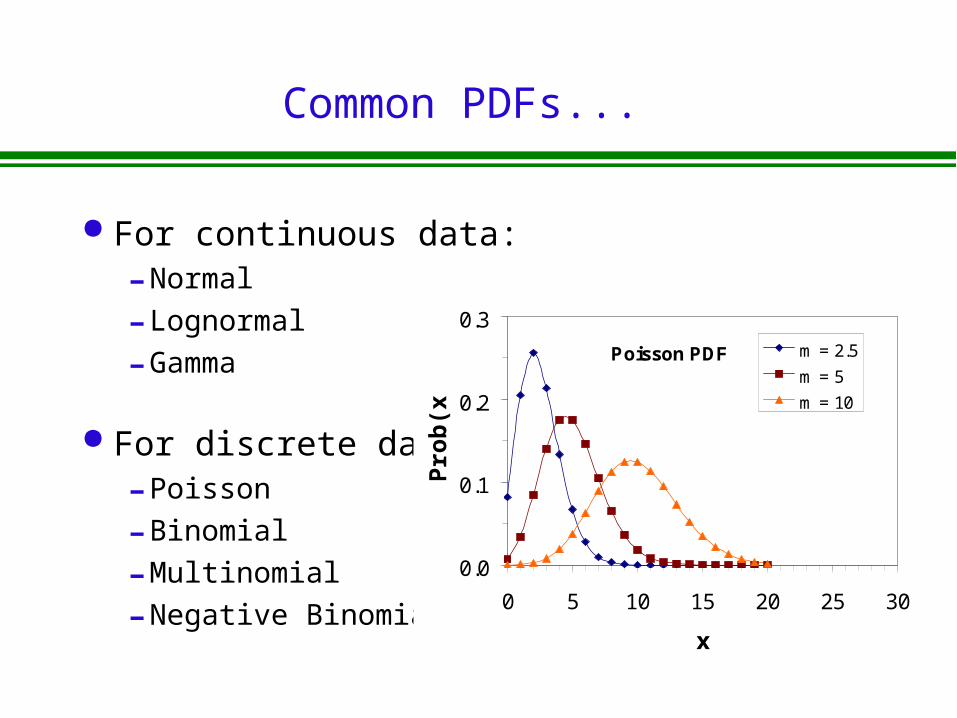
Common PDFs...

For continuous data:- Normal

- Lognormal

- Gamma

For discrete data:- Poisson

- Binomial

- Multinomial

- Negative Binomial

Poisson PDF

0.0

0.1

0.2

0.3

0 5 10 15 20 25 30

x

Pro

b(x

)

m = 2.5

m = 5

m = 10

Inference defined...

“a : the act of passing from one proposition, statement, or judgment considered as true to another whose truth is believed to follow from that of the former b : the act of passing from statistical sample data to generalizations (as of the value of population parameters) usually with calculated degrees of certainty”

Source: Merriam-Webster Online Dictionary

Statistical Inference...

... Typically concerns inferring properties of an unknown distribution from data generated by that distribution ...

Components:

-- Hypothesis testing

-- Point estimation

-- Model comparison

Probability and Inference

How do you choose the “correct inference” from your data, given inevitable uncertainty and error?

Can you assign a probability to your certainty in the correctness of a given inference?- (hint: if this is really important to you, then you

should consider becoming a Bayesian, as long as you can accept what I consider to be some fairly objectionable baggage…)

Assigning Probabilities to Hypotheses

Unfortunately, hypotheses (or even different parameter estimates) can not generally be treated as “data” (outcomes of trials)

Statisticians have debated alternate solutions to this problem for centuries- (with no generally agreed upon solution)

One Way Out: Classical “Frequentist” Statistics and Tests of Null Hypotheses

Probability is defined in terms of the outcome of a series of repeated trials..

Hypothesis testing via “significance” of pre-defined “statistics” :- What is the probability of observing a particular value of a

predefined test statistic, given an assumed hypothesis about the underlying scientific model, and assumptions about the probability model of the test statistic...

- Hypotheses are never “accepted”, but are “rejected” (categorically) if the probability of obtaining the observed value of the test statistic is very small (“p-value”)

An Implicit Assumption

The data are an approximate “sample” of an underlying “true” reality –

i.e., there is a true population mean, and the sample provides an estimate of it...

An example: Student’s “t” statistic

ns

uxt

/

Where u = hypothesized population mean

n = sample size s2 = sample variance

2

1

2 )(1

1xx

ns

n

ii

x= estimated sample mean

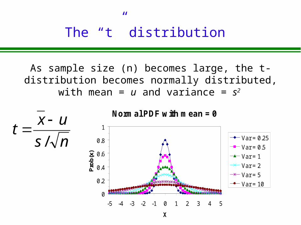
The “t” distribution

As sample size (n) becomes large, the t-distribution becomes normally distributed, with mean = u and

variance = s2

Normal PDF with mean = 0

0

0.2

0.4

0.6

0.8

1

-5 -4 -3 -2 -1 0 1 2 3 4 5

X

Pro

b(x

)

Var = 0.25

Var = 0.5

Var = 1

Var = 2

Var = 5

Var = 10

ns

uxt

/

Limitations of Frequentist Statistics

Do not provide a means of measuring relative strength of observational support for alternate hypotheses (merely helps decide when to “reject” individual hypotheses in comparison to a single “null” hypothesis...)- So you conclude the slope of the line is not = 0.

How strong is your evidence that the slope is really 0.45 vs. 0.50?

Extremely non-intuitive: just what is a “confidence interval” anyway...

Confidence Intervals

“...If a series of samples are drawn and the mean of each calculated, 95% of the means would be expected to fall within the range of two* standard errors above and two below the mean of these means...”

Source: http://bmj.bmjjournals.com/collections/statsbk/4.shtml

*actually, 1.96

A typical definition:

Standard Normal Distribution

0

0.1

0.2

0.3

0.4

0.5

-3 -2 -1 0 1 2 3

Standard Error of the Mean

Pro

babi

lity

cumulative prob. = 95%

The “null hypothesis” approach

When and where is “strong inference” really useful?

When is it just an impediment to progress?

Stephens et al. 2005. Information theory and hypothesis testing: a call for pluralism. Journal of Applied Ecology 42:4-12.

Platt, J. R. 1964. Strong inference. Science 146:347-353

Chamberlain’s alternative: multiple working hypotheses

Science rarely progresses through a series of dichotomously branched decisions…

Instead, we are constantly trying to choose among a large set of alternate hypotheses- Concept is very old, but the computational

power needed to adopt this approach has only recently become available…

Chamberlain, T. C. 1890. The method of multiple working hypotheses. Science 15:92.

Hypothesis testing and “significance”

Nester’s (1996) Creed:

•TREATMENTS: all treatments differ•FACTORS: all factors interact•CORRELATIONS: all variables are correlated•POPULATIONS: no two populations are identical in any respect•NORMALITY: no data are normally distributed•VARIANCES: variances are never equal•MODELS: all models are wrong•EQUALITY: no two numbers are the same•SIZE: many numbers are very small

Nester, M. R. 1996. An applied statistician’s creed. Applied Statistician 45:401-410

Hypothesis testing vs. estimation

“The problem of estimation is of more central importance, (than hypothesis testing).. for in almost all situations we know that the effect whose significance we are measuring is perfectly real, however small; what is at issue is its magnitude.” (Edwards, 1992, pg. 2)“An insignificant result, far from telling us that the effect is non-existent, merely warns us that the sample was not large enough to reveal it.” (Edwards, 1992, pg. 2)

Hypothesis testing and probability: the likelihood compromise

Probability (of the data) can not generally be used directly to test alternate hypotheses (about parameters)...

Fisher and the concept of “Likelihood”...http://www.economics.soton.ac.uk/staff/aldrich/fisherguide/prob+lik.htm“Likelihood and Probability in R. A. Fisher’s Statistical Methods for Research Workers” (John Aldrich) A good summary of the evolution of Fisher’s ideas on probability, likelihood, and inference… Contains links to PDFs of Fisher’s early papers… A second page shows the evolution of his ideas through changes in successive editions of Fisher’s books…

)|()|( xPxP

The “Likelihood Principle”

)|()|( xPxL

In plain English: “The likelihood (L) of the set of parameters (θ) (in the scientific model), given an observation (x) is proportional to the probability of observing the data, given the parameters...”

{and this probability is something we can calculate, using the appropriate underlying probability model (i.e. a PDF)}

Calculating Likelihood and Log-Likelihood for Datasets

)|(|1

n

iixgXLLikelihood

For i = 1..n independent observations, and a vector X of observations (xi):

Logarithms are easier to work with, so...

n

iixgXL

1

)|(ln|ln likelihood-Log

)|( ixgwhere is the PDF of the appropriate probability model

Likelihood “Surfaces”

The variation in likelihood for any given set of parameter values defines a likelihood “surface”...

For a model with just 1 parameter, the surface is simply a curve:

-155

-153

-151

-149

-147

2 2.1 2.2 2.3 2.4 2.5 2.6 2.7 2.8

Parameter Estimate

Lo

g-L

ikel

iho

od

“Support” and “Support Limits”

Log-likelihood = “Support” (Edwards 1992)

-155

-153

-151

-149

-147

2 2.1 2.2 2.3 2.4 2.5 2.6 2.7 2.8

Parameter Estimate

Lo

g-L

ike

liho

od

2-unit support interval

Maximum likelihood estimate

Models, Truth, and “Full Reality”(The Burnham and Anderson

view...)

“We believe that “truth” (full reality) in the biological sciences has essentially infinite dimension, and hence ... cannot be revealed with only ... finite data and a “model” of those data...

... We can only hope to identify a model that provides a good approximation to the data available.”

(Burnham and Anderson 2002, pg. 20)

“Thus, our general problem is to assess the relative merits of rival hypotheses in the light of observational or experimental data that bear upon them....” (Edwards, pg 1).

The crux of the problem...

Edwards, A.W.F. 1992. Likelihood. Expanded Edition. Johns Hopkins University Press.

The most important point of the course…

Any hypothesis test can be framed as a comparison of alternate models…

(and being free of the constraints imposed by the alternate models embedded in classical statistical tests is perhaps the

most important benefit of the likelihood approach…)

Example: Analysis of Covariance

A traditional ANCOVA model (homogeneous slopes):

What is restrictive about this model?

How would you generalize this in a likelihood framework?- What alternate models are you testing with the standard

frequentist statistics?

- What more general alternate models might you like to test?

groups 1..njfor

bxay iiji

“It will not be sufficient, when faced with a mass of observations, to plead special creation, even though, as we shall see, such a hypothesis commands a higher numerical likelihood than any other.”

(Edwards, 1992, pg. 1, in explaining the need for a rigorous basis for scientific inference, given uncertainty in nature...)

But is likelihood enough?

The importance of seeking simple answers...

The “full” model

What I irreverently call the “god” model: everything is the way it is because it is…

In statistical terms, this is simply a model with as many parameters as observations

- i.e.: xi = θiThis will always be the model with the highest likelihood!(but it won’t be the most parsimonious)…

Parsimony, Ockham’s razor, and drawing elephants...

William of Ockham (1285-1349):

“Pluralitas non est ponenda sine neccesitate”

“entities should not be multiplied unnecessarily”

“Parsimony: ... 2 : economy in the use of means to an end; especially : economy of explanation in conformity with Occam's razor” (Merriam-Webster Online Dictionary)

So how many parameters DOES it take to draw an elephant...?*

*30 would “carry a chemical engineer into preliminary design” (Wel, 1975) (cited in B&A, pg 30)

Information Theory perspective:

“How much information is lost when using a simple model to approximate reality?”

Answer: the Kullback-Leibler Distance (generally unknowable)

More Practical Answer: Akaike’s Information Criterion (AIC) identifies the model that minimizes KL distance KxLAIC 2)|(ln(2

The brave new world…

Science is the development of simplified models as explanations (approximations) of reality…

The “quality” of the explanation (the model) will be a balance of many factors (both quantitative and qualitative)