likelihood-based approaches to modeling the neural code

3Likelihood-Based Approaches toModeling the Neural CodeJonathan Pillow

One of the central problems in systems neuroscience is that of characteriz-ing the functional relationship between sensory stimuli and neural spike re-sponses. Investigators call this the neural coding problem, because the spiketrains of neurons can be considered a code by which the brain represents infor-mation about the state of the external world. One approach to understandingthis code is to build mathematical models of the mapping between stimuli andspike responses; the code can then be interpreted by using the model to pre-dict the neural response to a stimulus, or to decode the stimulus that gave riseto a particular response. In this chapter, we will examine likelihood-based ap-proaches, which use the explicit probability of response to a given stimulusfor both fitting the model and assessing its validity. We will show how thelikelihood can be derived for several types of neural models, and discuss theo-retical considerations underlying the formulation and estimation of such mod-els. Finally, we will discuss several ideas for evaluating model performance,including time-rescaling of spike trains and optimal decoding using Bayesianinversion of the likelihood function.

3.1 The Neural Coding Problem

Neurons exhibit stochastic variability. Even for repeated presentations of afixed stimulus, a neuron’s spike response cannot be predicted with certainty.Rather, the relationship between stimuli and neural responses is probabilistic.Understanding the neural code can therefore be framed as the problem of de-termining p(y|x), the probability of response y conditional on a stimulus x. Fora complete solution, we need to be able compute p(y|x) for any x, meaning adescription of the full response distribution for any stimulus we might presentto a neuron. Unfortunately, we cannot hope to get very far trying to measurethis distribution directly, due to the high dimensionality of stimulus space (e.g.,the space of all natural images) and the finite duration of neurophysiology ex-periments. Figure 3.1 shows an illustration of the general problem.

A classical approach to the neural coding problem has been to restrict at-

54 3 Likelihood-Based Approaches to Modeling the Neural Code Jonathan Pillow

......

p(y|x2)

x1

x2

p(y|x1)???x ystimulus response

p(y|x)goal:

Neural Coding Problem

Figure 3.1 Illustration of the neural coding problem. The goal is to find a modelmapping x to y that provides an accurate representation of the conditional distribu-tion p(y|x). Right: Simulated distribution of neural responses to two distinct stimuli,x1 and x2 illustrating (1) stochastic variability in responses to a single stimulus, and (2)that the response distribution changes as a function of x. A complete solution involvespredicting p(y|x) for any x.

tention to a small, parametric family of stimuli (e.g., flashed dots, movingbars, or drifting gratings). The motivation underlying this approach is theidea that neurons are sensitive only to a restricted set of stimulus features, andthat we can predict the response to an arbitrary stimulus simply by knowingthe response to these features. If x{ψ} denotes a parametric set of features towhich a neuron modulates its response, then the classical approach posits thatp(y|x) ≈ p(y|xψ), where xψ is the stimulus feature that most closely resemblesx.

Although the “classical" approach to neural coding is not often explicitlyframed in this way, it is not so different in principle from the “statistical mod-eling" approach that has gained popularity in recent years, and which we pur-sue here. In this framework, we assume a probabilistic model of the neural re-sponse, and attempt to fit the model parameters θ so that p(y|x, θ), the responseprobability under the model, provides a good approximation to p(y|x). Al-though the statistical approach is often applied using stimuli drawn stochasti-cally from a high-dimensional ensemble (e.g. Gaussian white noise) rather thana restricted parametric family (e.g. sine gratings), the goals are essentially sim-ilar: to find a simplified and computationally tractable description of p(y|x).The statistical framework differs primarily in its emphasis on detailed quanti-tative prediction of spike responses, and in offering a unifying mathematicalframework (likelihood) for fitting and validating models.

3.2 Model Fitting with Maximum Likelihood 55

3.2 Model Fitting with Maximum Likelihood

Let us now turn to the problem of using likelihood for fitting a model of anindividual neuron’s response. Suppose we have a set of stimuli x = {xi} anda set of spike responses y = {yi} obtained during a neurophysiology experi-ment, and we would like to fit a model that captures the mapping from x toy. Given a particular model, parametrized by the vector θ, we can apply atool from classical statistics known as maximum likelihood to obtain an asymp-totically optimal estimate of θ. For this, we need an algorithm for computingp(y|x, θ), which, considered as a function of θ, is called the likelihood of the data.The maximum likelihood (ML) estimate θ̂ is the set of parameters under whichthese data are most probable, or the maximizer of the likelihood function:

θ̂ = arg maxθ

p(y|x, θ). (3.1)

Although this solution is easily stated, it is unfortunately the case that formany models of neural response (e.g. detailed biophysical models such asHodgkin-Huxley) it is difficult or impossible to compute likelihood. Moreover,even when we can find simple algorithms for computing likelihood, maximiz-ing it can be quite difficult; in most cases, θ lives in a high-dimensional space,containing tens to hundreds of parameters (e.g. describing a neuron’s receptivefield and spike-generation properties). Such nonlinear optimization problemsare often intractable.

In the following sections, we will introduce several probabilistic neural spikemodels, derive the likelihood function for each model, and discuss the factorsaffecting ML estimation of its parameters. We will also compare ML with stan-dard (e.g. moment-based) approaches to estimating model parameters.

3.2.1 The LNP Model

One of the best-known models of neural response is the linear-nonlinear-Poisson(LNP) model, which is alternately referred to as the linear-nonlinear “cascade”model. The model, which is schematized in the left panel of figure 3.2, consistsof a linear filter (k), followed by a point nonlinearity (f ), followed by Pois-son spike generation. Although many interpretations are possible, a simpledescription of the model’s components holds that:

• k represents the neuron’s space-time receptive field, which describes howthe stimulus is converted to intracellular voltage;

• f describes the conversion of voltage to an instantaneous spike rate, ac-counting for such nonlinearities as rectification and saturation;

• instantaneous rate is converted to a spike train via an inhomogeneous Pois-son process.


The parameters of this model can be written as θ = {k, φf}, where φf are theparameters governing f . Although the LNP model is not biophysically realis-tic (especially the assumption of Poisson spiking), it provides a compact andreasonably accurate description of average responses, e.g., peri-stimulus timehistogram (PSTH), in many early sensory areas.

10 1 0 00 0 0 1 00 10 10 000 000 0 0 00 0

time

Response

...

...

...

...

dependency structure

Stimulus

Poisson

spiking

nonlinearity

linear filter

k f

LNP model

Figure 3.2 Schematic and dependency structure of the linear-nonlinear-Poissonmodel. Left: LNP model consists of a linear filter k, followed by a point nonlinearityf , followed by Poisson spike generation. Right: Depiction of a discretized white noiseGaussian stimulus (above) and spike response (below). Arrows indicate the causal de-pendency entailed by the model between portions of the stimulus and portions of theresponse. The highlighted gray box and gray oval show this dependence for a singletime bin of the response, while gray boxes and arrows indicate the (time-shifted) de-pendency for neighboring bins of the response. As indicated by the diagram, all timebins of the response are conditionally independent given the stimulus (equation (3.2)).

Another reason for the popularity of the LNP model is the existence of asimple and computationally efficient fitting algorithm, which consists in usingspike-triggered average (STA) as an estimate for k and a simple histogram pro-cedure to estimate φf (see [6, 8]). It is a well-known result that the STA (or“reverse correlation”) gives an unbiased estimate of the direction of k (i.e. theSTA converges to αk, for some unknown α) if the raw stimulus distributionp(x) is spherically symmetric, and f shifts the mean of the spike-triggered en-semble away from zero (i.e. the expected STA is not the zero vector) [7, 15].However, the STA does not generally provide an optimal estimate of k, exceptin a special case we will examine in more detail below [16].

First, we derive the likelihood function of the LNP model. The right panel offigure 3.2 shows the dependency structure (also known as a graphical model)between stimulus and response, where arrows indicate conditional dependence.For this model, the bins of the response are conditionally independent of oneanother given the stimulus, an essential feature of Poisson processes, whichmeans that the probability of the entire spike train factorizes as

p(y|x, θ) =∏

i

p(yi|xi, θ), (3.2)


where yi is the spike count in the ith time bin, and xi is the stimulus vectorcausally associated with this bin. Equation (3.2) asserts that the likelihood ofthe entire spike train is the product of the single-bin likelihoods. Under thismodel, single-bin likelihood is given by the Poisson distribution with rate pa-rameter ∆f(k·xi), where k·xi, is the dot product of k with xi and ∆ is the widthof the time bin. The probability of having yi spikes in the ith bin is therefore

p(yi|xi, θ) =1yi!

[∆f(k · xi)]yi e−∆f(k·xi), (3.3)

and the likelihood of the entire spike train can be rewritten as:

p(y|x, θ) = ∆n∏

i

f(k · xi)yi

yi!e−∆f(k·xi), (3.4)

where n is the total number of spikes.We can find the ML estimate θ̂ = {k̂, φ̂f} by maximizing the log of the likeli-

hood function (which is monotonically related to likelihood), and given by

log p(y|x, θ) =∑

i

yi log f(k · xi)−∆∑

i

f(k · xi) + c, (3.5)

where c is a constant that does not depend on k or f . Because there is an extradegree of freedom between the amplitude of k and input scaling of f , we canconstrain k to be a unit vector, and consider only the angular error in estimatingk. By differentiating the log-likelihood with respect to k and setting it to zero,we find that the ML estimate satisfies:

λk̂ =∑

i

yif ′(k̂ · xi)f(k̂ · xi)

xi −∆∑

i

f ′(k̂ · xi)xi, (3.6)

where λ is a Lagrange multiplier introduced to constrain k to be a unit vec-tor. As noted in [16], the second term on the right hand converges to a vectorproportional to k if the stimulus distribution p(x) is spherically symmetric. (Itis the expectation over p(x) of a function radially symmetric around k.) If wereplace this term by its expectation, we are left with just the first term, whichis a weighted STA, since yi is the spike count and xi is the stimulus precedingthe ith bin. This term is proportional to the (ordinary) STA if f ′/f is constant,which occurs only when f(z) = eaz+b.

Therefore, the STA corresponds to the ML estimate for k whenever f is ex-ponential; conversely, if f differs significantly from exponential, equation (3.6)specifies a different weighting of the spike-triggered stimuli, and the tradi-tional STA is suboptimal. Figure 3.3 illustrates this point with a comparisonbetween the STA and the ML estimate for k on spike trains simulated usingthree different nonlinearities. In the simulations, we found the ML estimate bydirectly maximizing log-likelihood (equation (3.5)) for both k and φf , begin-ning with the STA as an initial estimate for k. As expected, the ML estimateoutperforms the STA except when f is exponential (rightmost column).


-2 0 2 -2 0 2-2 0 2

0

50

100

filter output

0.25 0.5 1 2 4 8 16

0

5

10

15

20

time (min)

recitified-linear

0

50

100

filter output

0.25 0.5 1 2 4 8 16

0

10

20

30

time (min)

exponential

0

50

100

ra

te

(sp

/s)

filter output

0.25 0.5 1 2 4 8 16

0

10

20

30

40

time (min)

e

rro

r (d

e

g

)

STA

ML

linear

nonlinearity:

convergence:

Figure 3.3 Comparison of spike-triggered average (STA) and maximum likelihood(ML) estimates of the linear filter k in an LNP model. Top row: three different typesof nonlinearity f : a linear function (left), a half-wave rectified linear function (middle),and an exponential. For each model, the true k was a 20-tap temporal filter with bipha-sic shape similar to that found in retinal ganglion cells. The stimulus was temporalGaussian white noise with a frame rate of 100 Hz, and k was normalized so that filteroutput had unit standard deviation. Bottom row: Plots show the convergence behaviorfor each model, as a function of the amount of data collected. Error is computed as theangle between the estimate and the true k, averaged over 100 repeats at each stimuluslength.

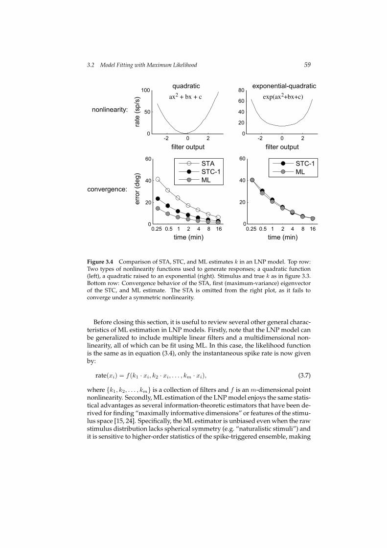
Figure 3.4 shows a similar analysis comparing ML to an estimator derivedfrom spike-triggered covariance (STC) analysis, which uses the principal eigen-vector of the STC matrix to estimate k. Recent work has devoted much atten-tion to fitting LNP models with STC analysis, which is relevant particularly incases where the f is approximately symmetric [10, 22, 26, 1, 25, 3, 23]. The leftcolumn of figure 3.4 shows a simulation where f is a quadratic, shifted slightlyfrom the origin so that both the STA and the first eigenvector of the STC pro-vide consistent (asymptotically convergent) estimates of k. Both, however, aresignificantly outperformed by the ML estimator. Although it is beyond thescope of this chapter, a derivation similar to the one above shows that thereis an f for which the ML estimator and the STC estimate are identical. Therelevant f is a quadratic in the argument of an exponential, which can also berepresented as a ratio of two Gaussians (see [20] for a complete discussion).The right column of figure 3.4 shows results obtained with such a nonlinearity.If we used a similar nonlinearity in which the first term of the quadratic is neg-ative, e.g. f(x) = exp(−x2), then f produces a reduction in variance along k,and the STC eigenvector with the smallest eigenvalue is comparable to the MLestimate [20].


-2 0 2

0

50

100

ra

te

(sp

/s)

filter output

STA

STC-1

ML

0.25 0.5 1 2 4 8 16

0

20

40

60

time (min)

e

rro

r (d

e

g

)

-2 0 2

0

20

40

60

80

filter output

0.25 0.5 1 2 4 8 16

0

20

40

60

time (min)

STC-1

ML

ax2 + bx + c

exponential-quadratic

nonlinearity:

convergence:

quadratic

exp(ax2+bx+c)

Figure 3.4 Comparison of STA, STC, and ML estimates k in an LNP model. Top row:Two types of nonlinearity functions used to generate responses; a quadratic function(left), a quadratic raised to an exponential (right). Stimulus and true k as in figure 3.3.Bottom row: Convergence behavior of the STA, first (maximum-variance) eigenvectorof the STC, and ML estimate. The STA is omitted from the right plot, as it fails toconverge under a symmetric nonlinearity.

Before closing this section, it is useful to review several other general charac-teristics of ML estimation in LNP models. Firstly, note that the LNP model canbe generalized to include multiple linear filters and a multidimensional non-linearity, all of which can be fit using ML. In this case, the likelihood functionis the same as in equation (3.4), only the instantaneous spike rate is now givenby:

rate(xi) = f(k1 · xi, k2 · xi, . . . , km · xi), (3.7)

where {k1, k2, . . . , km} is a collection of filters and f is an m-dimensional pointnonlinearity. Secondly, ML estimation of the LNP model enjoys the same statis-tical advantages as several information-theoretic estimators that have been de-rived for finding “maximally informative dimensions” or features of the stimu-lus space [15, 24]. Specifically, the ML estimator is unbiased even when the rawstimulus distribution lacks spherical symmetry (e.g. “naturalistic stimuli”) andit is sensitive to higher-order statistics of the spike-triggered ensemble, making


it somewhat more powerful and more general than STA or STC analysis. Un-fortunately, ML also shares the disadvantages of these information-theoreticestimators: it is computationally intensive, difficult to use for recovering mul-tiple (e.g. > 2) filters (in part due to the difficulty of choosing an appropriateparametrization for f ), and cannot be guaranteed to converge to the true max-imum using gradient ascent, due to the existence of multiple local maxima inthe likelihood function.

We address this last shortcoming in the next two sections, which discussmodels constructed to have likelihood functions that are free from sub-optimallocal maxima. These models also introduce dependence of the response onspike-train history, eliminating a second major shortcoming of the LNP model,the assumption of Poisson spike generation.

3.2.2 Generalized Linear Model

The generalized linear model (or GLM), schematized in figure 3.5, generalizesthe LNP model to incorporate feedback from the spiking process, allowing themodel to account for history-dependent properties of neural spike trains suchas the refractory period, adaptation, and bursting [16, 27]. As shown in thedependency diagram (right panel of figure 3.5), the responses in distinct timebins are no longer conditionally independent given the stimulus; rather, eachbin of the response depends on some time window of the recent spiking activ-ity. Luckily, this does not prevent us from factorizing the likelihood, which cannow be written

p(y|x, θ) =∏

i

p(yi|xi, y[i−k : i−1], θ), (3.8)

where y[i−k : i−1] is the vector of recent spiking activity from time bin i − k toi− 1. This factorization holds because, by Bayes’ rule, we have

p(yi, y[i−k : i−1]|x, θ) = p(yi|y[i−k : i−1],x, θ)p(y[i−k : i−1]|x, θ), (3.9)

and we can apply this formula recursively to obtain equation (3.8). (Note, how-ever, that no such factorization is possible if we allow loopy, e.g. bidirectional,causal dependence between time bins of the response.)

Except for the addition of a linear filter, h, operating on the neuron’s spike-train history, the GLM is identical to the LNP model. We could therefore call itthe “recurrent LNP” model, although its output is no longer a Poisson process,due to the history-dependence induced by h. The GLM likelihood function issimilar to that of the LNP model. If we let

ri = f(k · xi + h · y[i−k : i−1]) (3.10)

denote the instantaneous spike rate (or “conditional intensity” of the process),then the likelihood and log-likelihood, following equation (3.4) and (3.5), are


Stimulus


Response

10 1 0 00 0 0 1 00 10 10 000 000 0 0 00 0

generalized linear model

f

spikingnonlinearitylinear filter

+

post-spike waveform

k f

h

Figure 3.5 Diagram and dependency structure of a generalized linear model. Left:Model schematic, showing the introduction of history-dependence in the model viaa feedback waveform from the spiking process. In order to ensure convexity of thenegative log-likelihood, we now assume that the nonlinearity f is exponential. Right:Graphical model of the conditional dependencies in the GLM. The instantaneous spikerate depends on both the recent stimulus and recent history of spiking.

given by:

p(y|x, θ) = ∆n∏

i

ryi

i

yi!e−∆ri (3.11)

log p(y|x, θ) =∑

i

yi log ri −∆∑

i

ri + c. (3.12)

Unfortunately, we cannot use moment-based estimators (STA and STC) toestimate k and h for this model, because the consistency of those estimatorsrelies on spherical symmetry of the input (or Gaussianity, for STC), which thespike-history input term y[i−k : i−1] fails to satisfy [15].

As mentioned above, a significant shortcoming of the ML approach to neu-ral characterization is that it may be quite difficult in practice to find the maxi-mum of the likelihood function. Gradient ascent fails if the likelihood functionis rife with local maxima, and more robust optimization techniques (like simu-lated annealing) are computationally exorbitant and require delicate oversightto ensure convergence.

One solution to this problem is to constrain the model so that we guaran-tee that the likelihood function is free from (non-global) local maxima. If wecan show that the likelihood function is log-concave, meaning that the negativelog-likelihood function is convex, then we can be assured that the only max-ima are global maxima. Moreover, the problem of computing the ML estimateθ̂ is reduced to a convex optimization problem, for which there are tractablealgorithms even in very high-dimensional spaces.

As shown by [16], the GLM has a concave log-likelihood function if the non-linearity f is itself convex and log-concave. These conditions are satisfied ifthe second-derivative of f is non-negative and the second-derivative of log f


is non-positive. Although this may seem like a restrictive set of conditions—itrules out symmetric nonlinearities, for example—a number of suitable func-tions seem like reasonable choices for describing the conversion of intracellularvoltage to instantaneous spike rate, for example:

• f(z) = max(z + b, 0)

• f(z) = ez+b

• f(z) = log(1 + ez+b),

where b is a single parameter that we also estimate with ML.Thus, for appropriate choice of f , ML estimation of a GLM becomes compu-

tationally tractable. Moreover, the GLM framework is quite general, and caneasily be expanded to include additional linear filters that capture dependenceon spiking activity in nearby neurons, behavior of the organism, or additionalexternal covariates of spiking activity. ML estimation of a GLM has been suc-cessfully applied to the analysis of neural spike trains in a variety of sensory,motor, and memory-related brain areas [9, 27, 14, 19].

3.2.3 Generalized Integrate-and-Fire Model

We now turn our attention to a dynamical-systems model of the neural re-sponse, for which the likelihood of a spike train is not so easily formulatedin terms of a conditional intensity function (i.e. the instantaneous probabilityof spiking, conditional on stimulus and spike-train history). Recent work hasshown that the leaky integrate-and-fire (IF) model, a canonical but simplifieddescription of intracellular spiking dynamics, can reproduce the spiking statis-tics of real neurons [21, 13] and can mimic important dynamical behaviors ofmore complicated models like Hodgkin-Huxley [11, 12]. It is therefore naturalto ask whether likelihood-based methods can be applied to models of this type.

Figure 3.6 shows a schematic diagram of the generalized IF model [16, 18],which is a close relative of the well-known spike response model [12]. Themodel generalizes the classical IF model so that injected current is a linear func-tion of the stimulus and spike-train history, plus a Gaussian noise current thatintroduces a probability distribution over voltage trajectories. The model dy-namics (written here in discrete time, for consistency) are given by

vi+1 − vi∆

= −1τ

(vi − vL) + (k · xi) + (h · y[i−k : i−1]) + σNi∆− 12 , (3.13)

where vi is the voltage at the ith time bin, which obeys the boundary conditionthat whenever vi ≥ 1, a spike occurs and vi is reset instantaneously to zero.∆ is the width of the time bin of the simulation, and Ni is a standard Gaus-sian random variable, drawn independently on each i. The model parametersk and h are the same as in the GLM: linear filters operating on the stimulusand spike-train history (respectively), and the remaining parameters are: τ ,the time constant of the membrane leak; vL, the leak current reversal potential;and σ, the amplitude of the noise.


10 1 0 00 0 0 1 00 10 10 000 000 0 0 00 0


0 50 100

0

0

time (ms)

p

(sp

ike

)

vo

lta

g

e

likelihood of a single ISI

i

leaky integrator

threshold

noise

post-spike

current

linear filter

k

hN

generalized IF model

Figure 3.6 Generalized integrate-and-fire model. Top: Schematic diagram of modelcomponents, including a stimulus filter k and a post-spike current h that is injected intoa leaky integrator following every spike, and independent Gaussian noise to accountfor response variability. Bottom left: Graphical model of dependency structure, show-ing that the likelihood of each interspike interval (ISI) is conditionally dependent ona portion of the stimulus and spike-train history prior to the interspike interval (ISI).Bottom right: Schematic illustrating how likelihood could be computed with MonteCarlo sampling. Black trace shows the voltage (and spike time) from simulating themodel without noise, while gray traces show sample voltage paths (to the first spiketime) with noise. The likelihood of the ISI is shown above, as a function of the spiketime (black trace). Likelihood of an ISI is equal to the fraction of voltage paths crossingthreshold at the true spike time.

The lower left panel of figure 3.6 depicts the dependency structure of themodel as it pertains to computing the likelihood of a spike train. In this case,we can regard the probability of an entire interspike interval (ISI) as depend-ing on a relevant portion of the stimulus and spike-train history. The lowerright panel shows an illustration of how we might compute this likelihood fora single ISI under the generalized GIF model using Monte Carlo sampling.Computing the likelihood in this case is also known as the “first-passage time”problem. Given a setting of the model parameters, we can sample voltage tra-


jectories from the model, drawing independent noise samples for each trajec-tory, and following each trajectory until it hits threshold. The gray traces showshow five such sample paths, while the black trace shows the voltage path ob-tained in the absence of noise. The probability of a spike occurring at the ith binis simply the fraction of voltage paths crossing threshold at this bin. The blacktrace (above) shows the probability distribution obtained by collecting the firstpassage times of a large number of paths. Evaluated at the actual spike, thisdensity gives the likelihood of the relevant ISI. Because of voltage reset follow-ing a spike, all ISIs are conditionally independent, and we can again write thelikelihood function as a product of conditionally independent terms:

p(y|x, θ) =∏tj

p(y[tj−1+1 : tj ]|x, y[0 : tj ], θ), (3.14)

where {tj} is the set of spike times emitted by the neuron, y[tj−1+1 : tj ] is theresponse in the set of time bins in the jth ISI, and y[0 : tj ] is the response duringtime bins previous to that interval.

The Monte Carlo approach to computing likelihood of a spike train can inprinciple be performed for any probabilistic dynamical-systems style model.In practice, however, such an approach would be unbearably slow and wouldlikely prove intractable, particularly since the likelihood function must be com-puted many times in order find the ML estimate for θ. However, for the gen-eralized IF model there exists a much more computationally efficient methodfor computing the likelihood function using the Fokker-Planck equation. Al-though beyond the scope of this chapter, the method works by “density prop-agation” of a numerical representation of the probability density over sub-threshold voltage, which can be quickly computed using sparse matrix meth-ods. More importantly, a recent result shows that the log-likelihood functionfor the generalized IF model, like that of the GLM, is concave. This means thatthe likelihood function contains a unique global maximum, and that gradientascent can be used to find the ML estimate of the model parameters (see [17]for a more thorough discussion). Recent work has applied the generalized IFmodel to the responses of macaque retinal ganglion cells using ML, showingthat it can be used to capture stimulus dependence, spike-history dependence,and noise statistics of neural responses recorded in vitro [18].

3.3 Model Validation

Once we have a used maximum likelihood to fit a particular model to a set ofneural data, there remains the important task of validating the quality of themodel fit. In this section, we discuss three simple methods for assessing thegoodness-of-fit of a probabilistic model using the same statistical frameworkthat motivated our approach to fitting.

3.3 Model Validation 65

3.3.1 Likelihood-Based Cross-Validation

Recall that the basic goal of our approach is to find a probabilistic model suchthat we can approximate the true probabilistic relationship between stimulusand response, p(y|x), by the model-dependent p(y|x, θ). Once we have fit θusing a set of training data, how can we tell if the model provides a good de-scription of p(y|x)? To begin with, let us suppose that we have two competingmodels, pA and pB , parametrized by θA and θB , respectively, and we wish todecide which model provides a better description of the data. Unfortunately,we cannot simply compare the likelihood of the data under the two models,pA(y|x, θA) vs. pB(y|x, θB), due to the problem of overfitting. Even thoughone model assigns the fitted data a higher likelihood than the other, it may notgeneralize as well to new data.

As a toy example of the phenomenon of overfitting, consider a data set con-sisting of 5 points drawn from a Gaussian distribution. Let model A be a singleGaussian, fit with the mean and standard deviation of the sample points (i.e.the ML estimate for this model). For model B, suppose that the data come froma mixture of five very narrow Gaussians, and fit this model by centering oneof these narrow Gaussians at each of the 5 sample points. Clearly, the secondmodel assigns higher likelihood to the data (because it concentrates all proba-bility mass near the sample points), but it fails to generalize–it will assign verylow probability to new data points drawn from the true distribution which donot happen to lie very near the five original samples.

This suggests a general solution to the problem of comparing models, whichgoes by the name cross-validation. Under this procedure, we generate a new setof “test” stimuli, x∗ and present them to the neuron to obtain a new set of spikeresponses y∗. (Alternatively, we could set aside a small portion of the data atthe beginning.) By comparing the likelihood of these new data sets under thetwo models, pA(y∗|x∗, θA) vs. pB(y∗|x∗, θB), we get a fair test of the models’generalization performance. Note that, under this comparison, we do not ac-tually care about the number of parameters in the two models: increasing thenumber of parameters in a model does not improve its ability to generalize. (Inthe toy example above, model B has more parameters but generalizes muchmore poorly. We can view techniques like regularization as methods for reduc-ing the effective number of parameters in a model so that overfitting does notoccur.) Although we may prefer a model with fewer parameters for aesthetic orcomputational reasons, from a statistical standpoint we care only about whichmodel provides a better account of the novel data.

3.3.2 Time-Rescaling

Another powerful idea for testing validity of a probabilistic model is to usethe model to convert spike times into a series of i.i.d. random variables. Thisconversion will only be successful if we have accurately modeled the proba-bility distribution of each spike time. This idea, which goes under the nametime-rescaling [5], is a specific application of the general result that we can con-


vert any random variable into a uniform random variable using its cumulativedensity function (CDF).

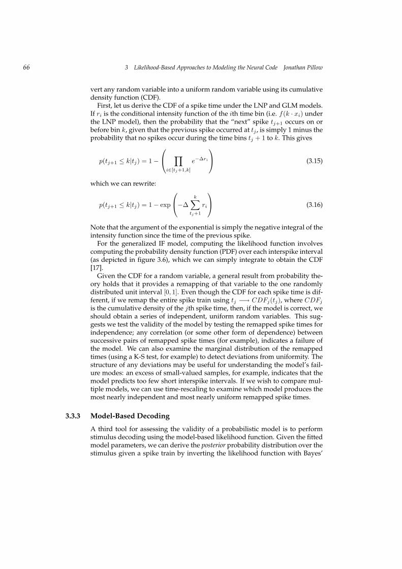
First, let us derive the CDF of a spike time under the LNP and GLM models.If ri is the conditional intensity function of the ith time bin (i.e. f(k · xi) underthe LNP model), then the probability that the “next” spike tj+1 occurs on orbefore bin k, given that the previous spike occurred at tj , is simply 1 minus theprobability that no spikes occur during the time bins tj + 1 to k. This gives

p(tj+1 ≤ k|tj) = 1− ∏

i∈[tj+1,k]

e−∆ri

(3.15)

which we can rewrite:

p(tj+1 ≤ k|tj) = 1− exp

−∆

k∑tj+1

ri

(3.16)

Note that the argument of the exponential is simply the negative integral of theintensity function since the time of the previous spike.

For the generalized IF model, computing the likelihood function involvescomputing the probability density function (PDF) over each interspike interval(as depicted in figure 3.6), which we can simply integrate to obtain the CDF[17].

Given the CDF for a random variable, a general result from probability the-ory holds that it provides a remapping of that variable to the one randomlydistributed unit interval [0, 1]. Even though the CDF for each spike time is dif-ferent, if we remap the entire spike train using tj −→ CDFj(tj), where CDFjis the cumulative density of the jth spike time, then, if the model is correct, weshould obtain a series of independent, uniform random variables. This sug-gests we test the validity of the model by testing the remapped spike times forindependence; any correlation (or some other form of dependence) betweensuccessive pairs of remapped spike times (for example), indicates a failure ofthe model. We can also examine the marginal distribution of the remappedtimes (using a K-S test, for example) to detect deviations from uniformity. Thestructure of any deviations may be useful for understanding the model’s fail-ure modes: an excess of small-valued samples, for example, indicates that themodel predicts too few short interspike intervals. If we wish to compare mul-tiple models, we can use time-rescaling to examine which model produces themost nearly independent and most nearly uniform remapped spike times.

3.3.3 Model-Based Decoding

A third tool for assessing the validity of a probabilistic model is to performstimulus decoding using the model-based likelihood function. Given the fittedmodel parameters, we can derive the posterior probability distribution over thestimulus given a spike train by inverting the likelihood function with Bayes’

3.3 Model Validation 67

rule:

p(x|y, θ) =p(y|x, θ)p(x)

p(y|θ) , (3.17)

where p(x) is the prior probability of the stimulus (which we assume to beindependent of θ), and the denominator is the probability of response y givenθ. We can obtain the most likely stimulus to have generated the response y bymaximizing the posterior for x, which gives the maximum a posteriori (MAP)estimate of the stimulus, which we can denote

x̂MAP = arg maxx

p(y|x, θ)p(x) (3.18)

since the denominator term p(y|θ) does not vary with x.For the GLM and generalized IF models, the concavity of the log-likelihood

function with respect to the model parameters also extends to the posteriorwith respect to the stimulus, since the stimulus interacts linearly with modelparameters k. Concavity of the log-posterior holds so long as the prior p(x)is itself log-concave (e.g. Gaussian, or any distribution of the form αe−(x/σ)γ

,with γ ≥ 1). This means that, for both of these two models, we can performMAP decoding of the stimulus using simple gradient ascent of the posterior.

If we wish to perform decoding with a specified loss function, for example,mean-squared error, optimal decoding can be achieved with Bayesian estima-tion, which is given by the estimator with minimum expected loss. In the caseof mean-squared error, this estimator is given by

x̂Bayes = E[x|y, θ], (3.19)

which is the conditional expectation of x, or the mean of the posterior distribu-tion over stimuli. Computing this estimate, however, requires sampling fromthe posterior distribution, which is difficult to perform without advanced sta-tistical sampling techniques, and is a topic of ongoing research.

Considered more generally, decoding provides an important test of modelvalidity, and it allows us to ask different questions about the nature of theneural code. Even though it may not be a task carried out explicitly in thebrain, decoding allows us to measure how well a particular model preservesthe stimulus-related information in the neural response. This is a subtle point,but one worth considering: we can imagine a model that performs worse un-der cross-validation or time-rescaling analyses, but performs better at decod-ing, and therefore gives a better account of the stimulus-related informationthat is conveyed to the brain. For example, consider a model that fails to ac-count for the refractory period (e.g. an LNP model), but which gives a slightlybetter description of the stimulus-related probability of spiking. This modelassigns non-zero probability to spike trains that violate the refractory period,thereby “wasting” probability mass on spike trains whose probability is actu-ally zero, and performing poorly under cross-validation. The model also per-forms poorly under time-rescaling, due to the fact that it over-predicts spike


rate during the refractory period. However, when decoding a real spike train,we do not encounter violations of the refractory period, and the “wasted” prob-ability mass affects only the normalizing term p(y|θ). Here, the model’s im-proved accuracy in predicting the stimulus-related spiking activity leads to aposterior that is more reliably centered around the true stimulus. Thus, eventhough the model fails to reproduce certain statistical features of the response,it provides a valuable tool for assessing what information the spike train car-ries about the stimulus, and gives a perhaps more valuable description of theneural code. Decoding may therefore serve as an important tool for validat-ing likelihood-based models, and a variety of exact or approximate likelihood-based techniques for neural decoding have been explored [28, 4, 2, 18].

3.4 Summary

We have shown how to compute likelihood and perform ML fitting of severaltypes of probabilistic neural models. In simulations, we have shown that MLoutperforms traditional moment-based estimators (STA and STC) when thenonlinear function of filter output does not have a particular exponential form.We have also discussed models whose log-likelihood functions are provablyconcave, making ML estimation possible even in high-dimensional parameterspaces and with non-Gaussian stimuli. These models can also be extended toincorporate dependence on spike-train history and external covariates of theneural response, such as spiking activity in nearby neurons. We have exam-ined several statistical approaches to validating the performance of a neuralmodel, which allow us to decide which models to use and to assess how wellthey describe the neural code.

In addition to the insight they provide into the neural code, the models wehave described may be useful for simulating realistic input to downstreambrain regions, and in practical applications such as neural prosthetics. Thetheoretical and statistical tools that we have described here, as well as the vastcomputational resources that make them possible, are still a quite recent de-velopment in the history of theoretical neuroscience. Understandably, theirachievements are still quite modest: we are some ways from a “complete”model that predicts responses to any stimulus (e.g., incorporating the effectsof spatial and multi-scale temporal adaptation, network interactions, and feed-back). There remains much work to be done both in building more power-ful and accurate models of neural responses, and in extending these models(perhaps in cascades) to the responses of neurons in brain areas more deeplyremoved from the periphery.

References

[1] Aguera y Arcas B, Fairhall AL (2003) What causes a neuron to spike? Neural Computa-tion, 15(8):1789–1807.

3.4 Summary 69

[2] Barbieri R, Frank L, Nguyen D, Quirk M, Solo V, Wilson M, Brown E (2004) DynamicAnalyses of Information Encoding in Neural Ensembles. Neural Computation, 16:277–307.

[3] Bialek W, de Ruyter van Steveninck R (2005) Features and dimensions: mo-tion estimation in fly vision. Quantitative Biology, Neurons and Cognition, arXiv:q-bio.NC/0505003.

[4] Brown E, Frank L, Tang D, Quirk M, Wilson M (1998) A statistical paradigm for neuralspike train decoding applied to position prediction from ensemble firing patterns ofrat hippocampal place cells. Journal of Neuroscience, 18:7411–7425.

[5] Brown E, Barbieri R, Ventura V, Kass R, Frank L (2002) The time-rescaling theorem andits application to neural spike train data analysis. Neural Computation, 14:325–346,2002.

[6] Bryant H, Segundo J (1976) Spike initiation by transmembrane current: a white-noiseanalysis. Journal of Physiology, 260:279–314.

[7] Bussgang J (1952) Crosscorrelation functions of amplitude-distorted gaussian signals.RLE Technical Reports, 216.

[8] Chichilnisky EJ (2001) A simple white noise analysis of neuronal light responses. Net-work: Computation in Neural Systems, 12:199–213.

[9] Chornoboy E, Schramm L, Karr A (1988) Maximum likelihood identification of neuralpoint process systems. Biological Cybernetics, 59:265–275.

[10] de Ruyter van Steveninck R, Bialek W (1988) Real-time performance of a movement-senstivive neuron in the blowfly visual system: coding and information transmissionin short spike sequences. Proceedings of Royal Society of London, B, 234:379–414.

[11] Gerstner W, Kistler W (2002) Spiking Neuron Models: Single Neurons, Populations, Plas-ticity. Cambridge, UK: University Press.

[12] Jolivet R, Lewis T, Gerstner W (2003) The spike response model: a framework topredict neuronal spike trains. Springer Lecture Notes in Computer Science, 2714:846–853.

[13] Keat J, Reinagel P, Reid R, Meister M (2001) Predicting every spike: a model for theresponses of visual neurons. Neuron, 30:803–817.

[14] Okatan M, Wilson M, Brown E (2005) Analyzing Functional Connectivity Using aNetwork Likelihood Model of Ensemble Neural Spiking Activity. Neural Computation,17:1927–1961.

[15] Paninski L (2003) Convergence properties of some spike-triggered analysis tech-niques. Network: Computation in Neural Systems, 14:437–464.

[16] Paninski L (2004) Maximum likelihood estimation of cascade point-process neuralencoding models. Network: Computation in Neural Systems, 15:243–262.

[17] Paninski L, Pillow J, Simoncelli E (2004) Maximum likelihood estimation of a stochas-tic integrate-and-fire neural model. Neural Computation, 16:2533–2561.

[18] Pillow JW, Paninski L, Uzzell VJ, Simoncelli EP, Chichilnisky EJ (2005) Prediction anddecoding of retinal ganglion cell responses with a probabilistic spiking model. Journalof Neuroscience, 25:11003–11013.

[19] Pillow JW, Shlens J, Paninski L, Chichilnisky EJ, Simoncelli EP (2005) Modeling thecorrelated spike responses of a cluster of primate retinal ganglion cells. SFN Abstracts,591.3.


[20] Pillow JW, Simoncelli EP (2006) Dimensionality reduction in neural models: aninformation-theoretic generalization of spike-triggered average and covariance anal-ysis. Journal of Vision, 6(4):414–428.

[21] Reich DS, Victor JD, Knight BW (1998) The power ratio and the interval map: spikingmodels and extracellular recordings. Journal of Neuroscience, 18:10090–10104.

[22] Schwartz O, Chichilnisky EJ, Simoncelli EP (2002) Characterizing neural gain controlusing spike-triggered covariance. In T G Dietterich, S Becker, and Z Ghahramani, ed-itors, Advances in Neural Information Processing Systems, volume 14, Cambridge, MA:MIT Press.

[23] Schwartz O, Pillow JW, Rust NC, Simoncelli EP (2006) Spike-triggered neural charac-terization. Journal of Vision, 6(4):484–507.

[24] Sharpee T, Rust N, Bialek W (2004) Analyzing neural responses to natural signals:maximally informative dimensions. Neural Computation, 16:223–250.

[25] Simoncelli E, Paninski L, Pillow J, Schwartz O (2004) Characterization of neural re-sponses with stochastic stimuli. In M. Gazzaniga, editor, The Cognitive Neurosciences,3rd edition, Cambridge, MA: MIT Press.

[26] Touryan J, Lau B, Dan Y (2002) Isolation of relevant visual features from randomstimuli for cortical complex cells. Journal of Neuroscience, 22:10811–10818.

[27] Truccolo W, Eden UT, Fellows MR, Donoghue JP, Brown EN (2004) A point processframework for relating neural spiking activity to spiking history, neural ensembleand extrinsic covariate effects. Journal of Neurophysiology, 93(2):1074–1089.

[28] Warland D, Reinagel P, Meister M (1997) Decoding visual information from a popu-lation retinal ganglion cells. Journal of Neurophysiology, 78:2336–2350.

Index

acausal, 122attention, 101attention, Bayesian model of, 249average cost per stage, 273

Bayes filter, 9Bayes rule, 298Bayes theorem, 6Bayesian decision making, 247Bayesian estimate, 8, 9Bayesian estimator, 114Bayesian inference, 235Bayesian network, 12belief propagation, 12, 235belief state, 285bell-shape, 111Bellman equation, 267Bellman error, 272bias, 113bit, 6

causal, 122coding, 112conditional probability, 4continuous-time Riccati equation, 281contraction mapping, 268contrasts, 94control gain, 282convolution code, 119convolution decoding, 121convolution encoding, 119correlation, 5costate, 274covariance, 4Cramér-Rao bound, 113, 115Cramér-Rao inequality, 11cross-validation, 65curse of dimensionality, 272

decision theory, 295decoding, 53, 112decoding basis function, 121deconvolution, 120differential dynamic programming,

282direct encoding, 117discounted cost, 273discrete-time Riccati equation, 282discrimination threshold, 116distributional codes, 253distributional population code, 117doubly distributional population code,

121Dynamic Causal Modeling (DCM), 103dynamic programming, 266

economics, 295EEG, 91encoding, 112entropy, 7estimation-control duality, 287Euler-Lagrange equation, 278evidence, 12expectation, 4expectation-maximization, 121extended Kalman filter, 285extremal trajectory, 275

filter gain, 284firing rate, 112Fisher Information, 11Fisher information, 115fMRI, 91Fokker-Planck equation, 286

gain of population activity, 118general linear model, 91

320 13 Bayesian Statistics and Utility Functions in Sensorimotor Control Konrad P. Körding and Daniel M. Wolpert

generalized linear model (GLM), 60graphical model, 12

Hamilton equation, 278Hamilton-Jacobi-Bellman equation,

271Hamiltonian, 275hemodynamic response function, 92hidden Markov model, 238, 285hierarchical inference, 255hyperparameter, 12hypothesis, 6

importance sampling, 285independence, 5influence function, 277information, 6information filter, 284information state, 285integrate-and-fire model, generalized,

62iterative LQG, 282Ito diffusion, 269Ito lemma, 271

joint probability, 4

Kalman filter, 9, 283Kalman smoother, 285Kalman-Bucy filter, 284kernel function, 119KL divergence, 8Kolmogorov equation, 286Kullback-Leiber divergence, 8

Lagrange multiplier, 276law of large numbers, 118Legendre transformation, 278likelihood, 6linear-quadratic regulator, 281log posterior ratio, 248loss function, 114

MAP, 8marginal likelihood, 12marginalization, 12Markov decision process, 269mass-univariate, 91maximum a posterior estimate, 8maximum a posteriori estimator, 67

maximum aposterior estimator, 287maximum entropy, 122maximum likelihood, 55, 114maximum likelihood estimate, 8maximum likelihood Estimator, 114maximum principle, 273mean, 4MEG, 91Mexican hat kernel, 120minimal variance, 114minimum-energy estimator, 287MLE, 8model selection, 12model-predictive control, 276motion energy, 118multiplicity, 121mutual information, 7

neural coding problem, 53

optimality principle, 266optimality value function, 266

particle filter, 9, 285Poisson distribution, 112Poisson noise, 115Poisson process, 56policy iteration, 267population code, 111population codes, 111population vector, 113posterior distribution, 114posterior probability, 6posterior probability mapping(PPM),

99preferred orientation, 111PrimerMarginal, 12prior distribution, 114prior probability, 6probabilistic population code, 118probability, 3probability density, 3probability distribution, 3product of expert, 122

random field, 122random field theory (RFT), 99Rauch recursion, 285recurrent network, linear, 240recurrent network, nonlinear, 242

Index 321

regularization, 11reverse correlation, 56rollout policy, 276

spike count, 112spike-triggered average (STA), 56spike-triggered covariance (STC), 58spiking neuron model, 243square-root filter, 284statistical parametric mapping (SPM),

99stimulus decoding, 113stimulus encoding, 112sufficient statistics, 285

temporally changing probability, 122time-rescaling, 53tuning curve, 111, 114

unbiased, 114unbiased estimate, 115uncertainty, 7, 116, 118, 120, 296unscented filter, 285utility, 296

value iteration, 267variance, 4, 113variance components , 97visual attention, 249visual motion detection, 244Viterbi algorithm, 287

Zakai’s equation, 286

likelihood-based approaches to modeling the neural code

Documents