lightwave refraction and its consequences: a viewpoint of...

$: Lightwave Refraction and Its Consequences: A Viewpoint of …cdn.intechopen.com/pdfs/33200/InTech-Lightwave_refraction_and_its... · 9 Lightwave Refraction and Its Consequences: A$
9

Lightwave Refraction and Its Consequences: A Viewpoint of Microscopic Quantum

Scatterings by Electric and Magnetic Dipoles

Chungpin Liao, Hsien-Ming Chang, Chien-Jung Liao, Jun-Lang Chen and Po-Yu Tsai National Formosa University (NFU)

Advanced Research and Business Laboratory (ARBL) Chakra Energetics, Ltd.

Taiwan

1. Introduction

In optics, it is well-known that when a visible light beam, e.g., traveling from air (or more

strictly, vacuum) into a piece of smooth flat glass at an angle relative to the normal of the

air-glass interface, some proportion of the light will be bounced off at the reflection angle

equal to the incident angle. However, when the light beam is with its oscillating electric field

parallel to the plane-of-incidence (POI, i.e., the plane constituted by both propagation

vectors of the incident and reflected light waves, as well as the interface normal vector)

(called the p-wave), there is a particular incident angle at which no bounce-off would occur.

This particular angle is known as the Brewster angle ( B ) (Hecht, 2002). In contrast, when

the light beam is with its electric field vector perpendicular to the plane-of-incidence (called

the s-wave), no such angle exists (Hecht, 2002). In fact, this is only true for uniform,

isotropic, and nonmagnetic (or equivalently, with its relative magnetic permeability ( r )

equal to unity at the optic frequency of interest) materials such as the above glass piece.

Indeed, it is known that for magnetic materials, there may instead exist Brewster angles for

the s-waves, while none for the p-waves (as will be demonstrated in Section 2).

Traditionally, whichever the case, the Brewster angle is a solid property of the material in

question with respect to a given light frequency of interest. Namely, there is a one-to-one

correspondence between the Brewster angle and the incident light frequency. However, it is

one of the purposes of this chapter to show that the Brewster angle of the material in hand

can in principle be modified into a new controllable variable, even dynamically, if a post-

process microscopic method called “dipole engineering” is applicable on that material.

Among its predictions, the traditionally fixed Brewster angle of a specific material now not

only becomes dependent on the density and orientation of incorporated permanent dipoles,

but also on the incident light intensity (more precisely, the incident wave electric field

strength). Further, two conjugated incident light paths would give rise to different refracted

wave powers (Liao et al., 2006).

www.intechopen.com

Advanced Photonic Sciences

216

In order to reveal the intricacies of the mechanism of the proposed permanent dipole engineering subsequently, existing important result of Doyle (Doyle, 1985) is first thoroughly detailed. That is, the Fresnel equations and Brewster angle formula are to be arrived at intuitively and rigorously obtained, by viewing all light-wave-induced dipole moments (including both electric and magnetic dipoles) as the microscopic sources causing the observed macroscopic optical phenomena at an interface, as compared to the traditional academic “Maxwell” approach ignoring the dipole picture. Then, equipped with such-developed intuitive and quantitative physical picture, the readers are then ready to appreciate the way those optically-responsive, permanent dipoles are externally implemented into a selected host matter and their rendered effects. Namely, the Brewster angle of a selected host material becomes alterable, likely at will, and ultimately new optical materials, devices and applications may emerge.

2. Brewster angle and “scattering” form of Fresnel equations

Arising from Maxwell’s equations (through assuming linear media and adopting monochromatic plane-waves expansion), Fresnel equations provide almost complete quantitative descriptions about the incident, reflected and transmitted waves at an interface, including information concerning energy distribution and phase variations among them (Hecht, 2002). Two of the Fresnel equations are relevant to reflections associated with both the p and s components (Hecht, 2002):

cos cos

cos cos

ss r i rt i t ri t

si rt i t ri ti

E n nr

n nE

(1)

cos cos

cos cos

pp r ri t i rt i t

pri t i rt i ti

E n nr

n nE

(2)

where E is the electric field, r is the relative magnetic permeability, 1/2r rn is the

index of refraction ( r being the relative dielectric coefficient), superscripts “p” and “s” stand for the p-wave and s-wave components, while subscripts “i”, “r” and “t” denote incident, reflected and transmitted components, respectively. When the incident angle ( i ) is equal to a particular value ( B ), one of the above reflection coefficients would vanish, then such value of the incident angle is known as the Brewster angle ( B ). Note that for the most familiar case in which the light wave is incident from vacuum onto a linear nonmagnetic medium ( 1r ), only the p-wave possesses a Brewster angle, not the s-wave.

In the following, to get ready for our proposed idea while without loss of generality, the medium on the incident side is designated to be vacuum (i.e., 1in ) for simplicity. In addition, to further facilitate our purpose, the Fresnel equations in the equivalent “scattering” form (due to Doyle) are retyped here (Doyle, 1985):

1 1 cos

2 cos sin

sin

prt

pr r r r t ii

i t i

t

E

E

(3)

www.intechopen.com

Lightwave Refraction and Its Consequences: A Viewpoint of Microscopic Quantum Scatterings by Electric and Magnetic Dipoles

217

1 1 cos

1 1 cos

sin

sin

pr r r r t ir

pr r r r t ii

t i

t i

E

E

(4)

1 1 cos

2 cos sin

sin

srt

sr r r r t ii

i t i

t

E

E

(5)

1 1 cos

1 1 cos

sin

sin

sr r r r t ir

sr r r r t ii

t i

t i

E

E

(6)

Namely, the right hand sides of Eq. (3)-(6) are in the form of D S, with D being the first

bracketed term, representing single dipole (electric and magnetic) oscillation; while S being

the second term, depicting the collective scattering pattern generated by the whole array of

dipoles. While S is nonzero, where D vanishes (Eq. (4) or (6)) is the condition for the

Brewster angle to arise either for the p-wave or the s-wave. That is (Doyle, 1985),

2tan1

p r r rB

r r

(7)

2tan1

r r rsB

r r

(8)

Note that if the medium is characterized by r r , only the s-wave may experience the

Brewster angle; while in the r r situation, only the p-wave can. Indeed, in the most

familiar case of light going from vacuum into a piece of glass whose 1r r , there is the

Brewster angle only for the p-wave.

In the following, an alternative derivation of the “scattering” form Fresnel equations (Eq. (4)-(6)) will be reproduced from (Doyle, 1985) in somewhat details, which stems from the viewpoint of treating induced microscopic (electric and magnetic) dipoles as the effective sources of macroscopic EM waves at the interface. Then, effective ways to implement the proposed permanent dipoles on a host material will be proposed, which will in principle allow us to achieve variant Brewster angles and thus to create novel materials, devices, even new applications.

3. ’’Scattering” form Fresnel equations from the dipole source viewpoint

Microscopically, all matters including optical materials are made of atoms or molecules, each of which further consists of a positive-charged nucleus (or nuclei) and some orbiting

www.intechopen.com


218

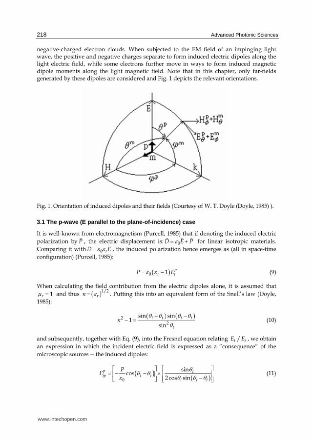
negative-charged electron clouds. When subjected to the EM field of an impinging light wave, the positive and negative charges separate to form induced electric dipoles along the light electric field, while some electrons further move in ways to form induced magnetic dipole moments along the light magnetic field. Note that in this chapter, only far-fields generated by these dipoles are considered and Fig. 1 depicts the relevant orientations.

Fig. 1. Orientation of induced dipoles and their fields (Courtesy of W. T. Doyle (Doyle, 1985) ).

3.1 The p-wave (E parallel to the plane-of-incidence) case

It is well-known from electromagnetism (Purcell, 1985) that if denoting the induced electric

polarization by P

, the electric displacement is: 0D E P for linear isotropic materials.

Comparing it with 0 rD E , the induced polarization hence emerges as (all in space-time

configuration) (Purcell, 1985):

0 1 pr tP E

(9)

When calculating the field contribution from the electric dipoles alone, it is assumed that

1r and thus 1/2rn . Putting this into an equivalent form of the Snell’s law (Doyle,

1985):

2

2

sin sin1

sin

i t i t

t

n

(10)

and subsequently, together with Eq. (9), into the Fresnel equation relating /t iE E , we obtain

an expression in which the incident electric field is expressed as a “consequence” of the

microscopic sources -- the induced dipoles:

0

sincos

2 cos sin

p tt iip

i t i

PE

(11)

www.intechopen.com


219

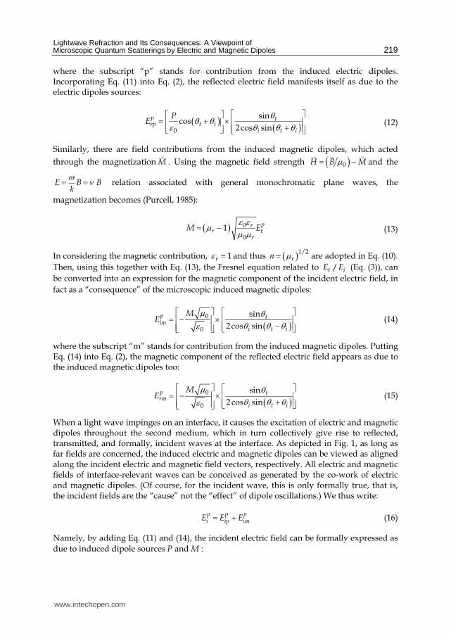
where the subscript “p” stands for contribution from the induced electric dipoles. Incorporating Eq. (11) into Eq. (2), the reflected electric field manifests itself as due to the electric dipoles sources:

0

sincos

2 cos sinp trp t i

i t i

PE

(12)

Similarly, there are field contributions from the induced magnetic dipoles, which acted

through the magnetization M

. Using the magnetic field strength 0H B M and the

E B Bk

relation associated with general monochromatic plane waves, the

magnetization becomes (Purcell, 1985):

0

0

1 prr t

r

M E (13)

In considering the magnetic contribution, 1r and thus 1/2rn are adopted in Eq. (10).

Then, using this together with Eq. (13), the Fresnel equation related to /t iE E (Eq. (3)), can

be converted into an expression for the magnetic component of the incident electric field, in

fact as a “consequence” of the microscopic induced magnetic dipoles:

0

0

sin

2 cos sin

p tim

i t i

ME

(14)

where the subscript “m” stands for contribution from the induced magnetic dipoles. Putting Eq. (14) into Eq. (2), the magnetic component of the reflected electric field appears as due to the induced magnetic dipoles too:

0

0

sin

2 cos sinp trm

i t i

ME

(15)

When a light wave impinges on an interface, it causes the excitation of electric and magnetic dipoles throughout the second medium, which in turn collectively give rise to reflected, transmitted, and formally, incident waves at the interface. As depicted in Fig. 1, as long as far fields are concerned, the induced electric and magnetic dipoles can be viewed as aligned along the incident electric and magnetic field vectors, respectively. All electric and magnetic fields of interface-relevant waves can be conceived as generated by the co-work of electric and magnetic dipoles. (Of course, for the incident wave, this is only formally true, that is, the incident fields are the “cause” not the “effect” of dipole oscillations.) We thus write:

p p pi ip imE E E (16)

Namely, by adding Eq. (11) and (14), the incident electric field can be formally expressed as

due to induced dipole sources P and M :

www.intechopen.com


220

0

0 0

sincos

2 cos sin

p tt ii

i t i

MPE

(17)

As a verification, if putting forms of these sources (i.e., Eq. (9) and (13) in which the induced

P and M are expressed in term of ptE ) back into Eq. (17), it is found that the obtained

transmission coefficient of the p-wave is exactly that of Eq. (3).

Similarly, conceiving the reflected electric field as:

p p pr rp rmE E E (18)

Adding Eq. (12) and (15), the reflected electric field appears as due to the induced dipole

sources P and M :

0

0 0

sincos

2 cos sinp tr t i

i t i

MPE

(19)

Similarly, putting forms of the dipoles sources (i.e., Eq. (9) and (13) in which P and M are

expressed in terms of ptE ) back into Eq. (19), and using the newly obtained p

iE vs. p

tE relation (i.e., Eq. (17)), it is found that the obtained reflection coefficient of the p-wave is

exactly that of Eq. (4), in “scattering” form.

3.2 The s-wave (E perpendicular to the plane-of-incidence) case

Likewise, following Fig. 1 again, we can also express the incident and reflected electric fields of the s-wave as due to those induced electric and magnetic dipoles:

0

0 0

sincos

2 cos sins ti t i

i t i

MPE

(20)

0

0 0

sincos

2 cos sins tr t i

i t i

MPE

(21)

and that the transmission and reflection coefficients are indeed found to be those of Eq. (5) and (6), respectively, in “scattering” form.

4. The proposed permanent dipoles engineering

4.1 Observations and inspirations

From the above elaboration, it becomes obvious that the electric and magnetic dipoles can be much more than mere pedagogical tools for picturing dielectrics and magnetics, as indeed proven by Doyle (Doyle, 1985). In fact, treating them as microscopic EM wave sources from the outset, the “scattering” form of Fresnel equations (i.e., Eq. (3)-(6)), and consequently, the Brewster angle formulas (Eq. (7) and (8)) can all be reproduced. Then, emerging from such

www.intechopen.com


221

details come our inspired purposes. Namely, by acquainting ourselves with the role played by these induced dipoles (or, the microscopic scattering sources), it is then intuitively straightforward to learn how new macroscopic optical phenomena, such as the new Brewster angle may be generated if extra anisotropic optically-responsive permanent dipoles were implemented onto the originally isotropic host material in discussion (Liao et al., 2006).

In other words, now the notions of P and M are further extended to include the total

effects resulting from both the induced and permanent dipoles.

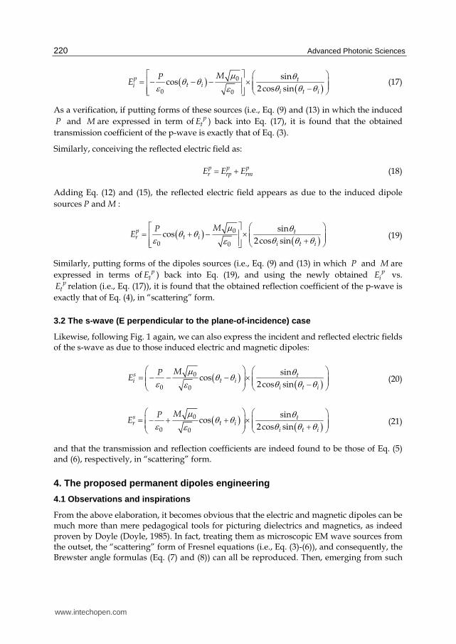
For instance, in Eq. (17), the cos t i factor multiplying on P (but not on M ) is due to

the fact that the induced polarization P (along ptE ) has only a fractional contribution to

piE determined by the vector projection as shown in Fig. 2, for the p-wave situation. Now, if

an external polarization vector 0P (as the collective result of many imposed electric

dipoles responding to the incident lightwave of radian frequency at the incident angle i )

is introduced within a host material, then, e.g., for the p-wave case, all electric dipoles’

contribution to piE (i.e., Eq. (17)) is now 0 0cos cosinduced i t iP P , or 0 0 01 cos cosp

r t i t iE P (see Fig. 2). Namely, there is now an additional

second anisotropic term resulting from externally imposed dipoles whose contribution may

not necessarily be less than the induced dipoles of the original isotropic host. Note that the

incident light-driven response of these externally imposed permanent dipoles is frequency

dependent, and therefore, the above 0P really stands for that amount of polarization at the

relevant optical frequency of interest and the lightwave’s incident angle i . In other words,

a “DC” polarization will never enter the above equation, and 0ptP E would be constant for

each specific i if the added dipoles, and hence the resultant polarization, are linear.

Fig. 2. P-wave configuration at the interface and the orientation of embedded permanent electric dipoles (Courtesy of W. T. Doyle (Doyle, 1985) ).

www.intechopen.com


222

Thus, if the dipole-engineered total contribution is recast in the traditional form, viz., 0 1 cosp

r t i tE , then it is clear that the modified relative dielectric coefficient is equivalently (Liao et al., 2006):

00

0

cos

cosi

r rpi tt

P

E

(22)

where 0 is the angle between the imposed extra polarization vector and the interface plane (see Fig. 2). Thus, by putting Eq. (22) into the p-wave Brewster angle formula (Eq. (7)), a new Brewster angle ( B ) would then emerge:

2tan1

p r r rB

r r

(23)

4.2 Justification of the effectiveness and meaningfulness of implementing optically-responsive dipoles

A justification of the effectiveness of the proposed permanent dipole engineering is straightforward by noting the following fact. Namely, had the original host material been transformed into a new material by adding in a considerable amount of certain second substance, then 0P in the above really would have stood for the extra induced dipole effect resulting from this second substance.

However, to this end, an inquiry may naturally arise as to whether the outcome of the proposed dipole-engineering approach being nothing more than having a material of multi-components from the outset. The answer is clearly no, and there are much more meaningful and practical intentions behind the proposed method. First of all, this is a controllable way to make new materials from known materials without having to largely mess around with typically complicated details of manufacturing processes pertaining to each involved material (if the introduced permanent dipoles are noble enough). Indeed, we have been routinely attempting to create various materials by combining multiple substances, and yet have also been very much limited by problems related to chemical compatibility, phase transition, in addition to many processing and economic considerations. Secondly, permanent dipole engineering would further allow delicate, precise means of manipulating the material properties, such as varying the dipole orientation to render desired optical performance on host materials of choice. Thirdly, all existing techniques known to influence dipoles can be readily applied on the now embedded dipoles to harvest new optical advantages, such as by electrically biasing the dipoles to adjust the magnitude of permanent dipole moment (in terms of 0P ) in the frequency range of interest.

4.3 Different refracted wave powers on two conjugated incident light paths

If, instead of picking the incidence from the left hand side as depicted in Fig. 2, a conjugate path, i.e., from the right hand side, is taken (see, Fig. 3), then the formula for Eq. (22) becomes (Liao et al., 2006):

00

0

cos

cosi

r rpt it

P

E

(24)

www.intechopen.com


223

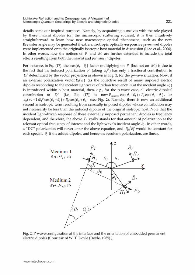
Unconventional Brewster angle can be found by Eq. (23) (p-wave case).

Fig. 3. P-wave configuration and the orientation of embedded permanent electric dipoles (Conjugated Incident Light Path, courtesy of W. T. Doyle (Doyle, 1985) ).

In other words, the traditionally fixed Brewster angle of a specific material now not only becomes dependent on the density and orientation of incorporated permanent dipoles, but also on the incident light intensity (more precisely, the incident wave electric field strength). Further, two conjugated incident light paths would give rise to different refracted wave powers (Liao et al., 2006), (Haus & Melcher, 1989).

4.4 The surface embedded with a thin distributed double layer

The traditional Fresnel equations in the electromagnetic theory have been used in determining the light power distribution at an interface joining two different media in general. They are known to base upon the so-called “no-jump conditions” ((Haus & Melcher, 1989), (Hecht, 2002)) wherein the interface-parallel components of the electric and magnetic fields of a plane wave continue seamlessly across the interface, respectively:

|| ||0 0E and H (25)

where a bQ Q Q stands for the discontinuity of the physical quantity Q by crossing from

the a side to the b side of the interface, and || (or ) is with respect to the interface plane.

The general configuration of light incidence can be decomposed into the p-wave and s-wave

situations. For the p-wave case, the lightwave’s electric field is on the plane of incidence

(POI) (see Fig. 4), and for the s-wave situation, it is pointing perpendicularly out of the POI.

www.intechopen.com


224

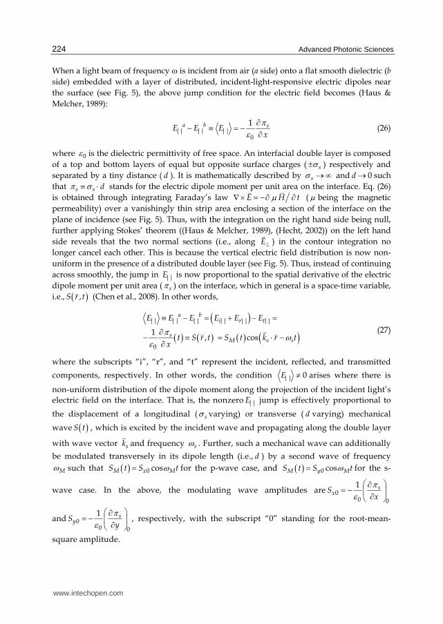
When a light beam of frequency is incident from air (a side) onto a flat smooth dielectric (b

side) embedded with a layer of distributed, incident-light-responsive electric dipoles near

the surface (see Fig. 5), the above jump condition for the electric field becomes (Haus &

Melcher, 1989):

|| || ||0

1a b sE E Ex

(26)

where 0 is the dielectric permittivity of free space. An interfacial double layer is composed

of a top and bottom layers of equal but opposite surface charges ( s ) respectively and

separated by a tiny distance ( d ). It is mathematically described by s and 0d such

that s s d stands for the electric dipole moment per unit area on the interface. Eq. (26)

is obtained through integrating Faraday’s law E H t ( being the magnetic

permeability) over a vanishingly thin strip area enclosing a section of the interface on the

plane of incidence (see Fig. 5). Thus, with the integration on the right hand side being null,

further applying Stokes’ theorem ((Haus & Melcher, 1989), (Hecht, 2002)) on the left hand

side reveals that the two normal sections (i.e., along E

) in the contour integration no

longer cancel each other. This is because the vertical electric field distribution is now non-

uniform in the presence of a distributed double layer (see Fig. 5). Thus, instead of continuing

across smoothly, the jump in ||E is now proportional to the spatial derivative of the electric

dipole moment per unit area ( s ) on the interface, which in general is a space-time variable,

i.e., ,S r t

(Chen et al., 2008). In other words,

|| || || || || ||

0

1, cos

a bi r t

sM s s

E E E E E E

t S r t S t k r tx

(27)

where the subscripts “i”, “r”, and “t” represent the incident, reflected, and transmitted

components, respectively. In other words, the condition || 0E arises where there is

non-uniform distribution of the dipole moment along the projection of the incident light’s

electric field on the interface. That is, the nonzero ||E jump is effectively proportional to

the displacement of a longitudinal ( s varying) or transverse ( d varying) mechanical

wave S t , which is excited by the incident wave and propagating along the double layer

with wave vector sk

and frequency s . Further, such a mechanical wave can additionally

be modulated transversely in its dipole length (i.e., d ) by a second wave of frequency

M such that 0 cosM x MS t S t for the p-wave case, and 0 cosM y MS t S t for the s-

wave case. In the above, the modulating wave amplitudes are 00 0

1 sxS

x

and 00 0

1 syS

y

, respectively, with the subscript “0” standing for the root-mean-

square amplitude.

www.intechopen.com


225

Fig. 4. (a) Refraction with p-wave incidence and (b) refraction with s-wave incidence.

Fig. 5. Surface integration of Faraday’s law enclosing a section of the double layer and regions above (a) and below (b) it.

www.intechopen.com


226

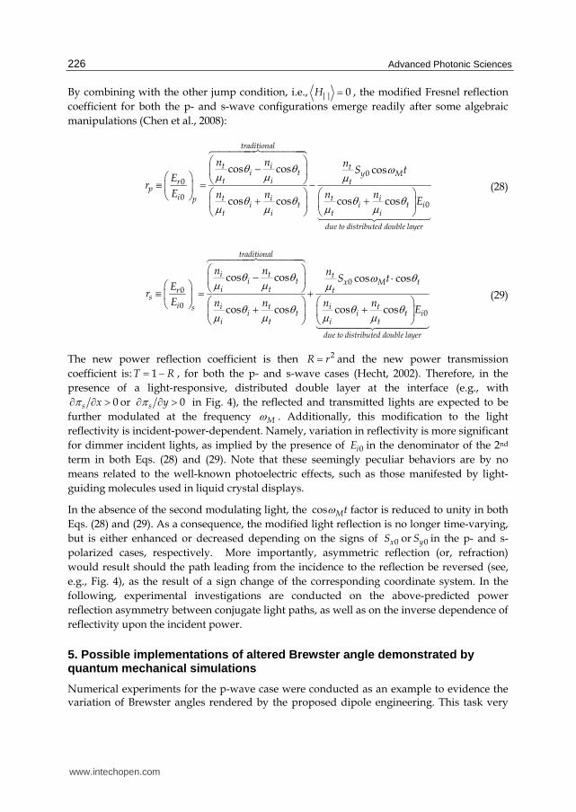
By combining with the other jump condition, i.e., || 0H , the modified Fresnel reflection

coefficient for both the p- and s-wave configurations emerge readily after some algebraic

manipulations (Chen et al., 2008):

00

00

cos cos cos

cos cos cos cos

traditional

t i ti t y M

t ir tp

i t i t ipi t i t i

t i t i

due to distributed double layer

n n nS t

Er

E n n n nE

(28)

00

00

cos cos cos cos

cos cos cos cos

traditional

i t ti t x M t

i tr ts

i i t i tsi t i t i

i t i t

due to distributed double layer

n n nS t

Er

E n n n nE

(29)

The new power reflection coefficient is then 2R r and the new power transmission

coefficient is: 1T R , for both the p- and s-wave cases (Hecht, 2002). Therefore, in the

presence of a light-responsive, distributed double layer at the interface (e.g., with

0s x or 0s y in Fig. 4), the reflected and transmitted lights are expected to be

further modulated at the frequency M . Additionally, this modification to the light

reflectivity is incident-power-dependent. Namely, variation in reflectivity is more significant

for dimmer incident lights, as implied by the presence of 0iE in the denominator of the 2nd

term in both Eqs. (28) and (29). Note that these seemingly peculiar behaviors are by no

means related to the well-known photoelectric effects, such as those manifested by light-

guiding molecules used in liquid crystal displays.

In the absence of the second modulating light, the cos Mt factor is reduced to unity in both

Eqs. (28) and (29). As a consequence, the modified light reflection is no longer time-varying,

but is either enhanced or decreased depending on the signs of 0xS or 0yS in the p- and s-

polarized cases, respectively. More importantly, asymmetric reflection (or, refraction)

would result should the path leading from the incidence to the reflection be reversed (see,

e.g., Fig. 4), as the result of a sign change of the corresponding coordinate system. In the

following, experimental investigations are conducted on the above-predicted power

reflection asymmetry between conjugate light paths, as well as on the inverse dependence of

reflectivity upon the incident power.

5. Possible implementations of altered Brewster angle demonstrated by quantum mechanical simulations

Numerical experiments for the p-wave case were conducted as an example to evidence the variation of Brewster angles rendered by the proposed dipole engineering. This task very

www.intechopen.com


227

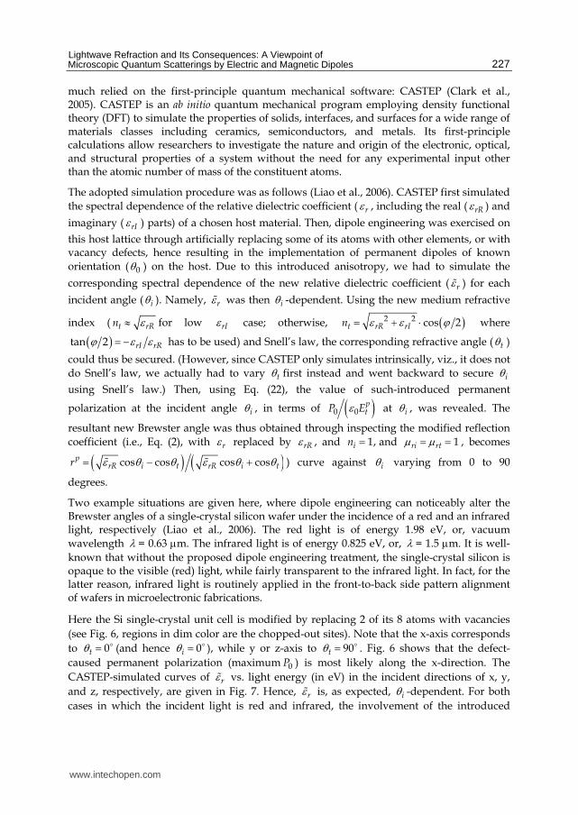
much relied on the first-principle quantum mechanical software: CASTEP (Clark et al., 2005). CASTEP is an ab initio quantum mechanical program employing density functional theory (DFT) to simulate the properties of solids, interfaces, and surfaces for a wide range of materials classes including ceramics, semiconductors, and metals. Its first-principle calculations allow researchers to investigate the nature and origin of the electronic, optical, and structural properties of a system without the need for any experimental input other than the atomic number of mass of the constituent atoms.

The adopted simulation procedure was as follows (Liao et al., 2006). CASTEP first simulated

the spectral dependence of the relative dielectric coefficient ( r , including the real ( rR ) and

imaginary ( rI ) parts) of a chosen host material. Then, dipole engineering was exercised on

this host lattice through artificially replacing some of its atoms with other elements, or with vacancy defects, hence resulting in the implementation of permanent dipoles of known

orientation ( 0 ) on the host. Due to this introduced anisotropy, we had to simulate the

corresponding spectral dependence of the new relative dielectric coefficient ( r ) for each

incident angle ( i ). Namely, r was then i -dependent. Using the new medium refractive

index ( t rRn for low rI case; otherwise, 2 2 cos 2t rR rIn where

tan 2 rI rR has to be used) and Snell’s law, the corresponding refractive angle ( t )

could thus be secured. (However, since CASTEP only simulates intrinsically, viz., it does not

do Snell’s law, we actually had to vary t first instead and went backward to secure i

using Snell’s law.) Then, using Eq. (22), the value of such-introduced permanent

polarization at the incident angle i , in terms of 0 0ptP E at i , was revealed. The

resultant new Brewster angle was thus obtained through inspecting the modified reflection

coefficient (i.e., Eq. (2), with r replaced by rR , and 1,in and 1ri rt , becomes cos cos cos cosprR i t rR i tr ) curve against i varying from 0 to 90

degrees.

Two example situations are given here, where dipole engineering can noticeably alter the Brewster angles of a single-crystal silicon wafer under the incidence of a red and an infrared light, respectively (Liao et al., 2006). The red light is of energy 1.98 eV, or, vacuum

wavelength = 0.63 m. The infrared light is of energy 0.825 eV, or, = 1.5 m. It is well-

known that without the proposed dipole engineering treatment, the single-crystal silicon is opaque to the visible (red) light, while fairly transparent to the infrared light. In fact, for the latter reason, infrared light is routinely applied in the front-to-back side pattern alignment of wafers in microelectronic fabrications.

Here the Si single-crystal unit cell is modified by replacing 2 of its 8 atoms with vacancies

(see Fig. 6, regions in dim color are the chopped-out sites). Note that the x-axis corresponds

to 0t (and hence 0i ), while y or z-axis to 90t . Fig. 6 shows that the defect-

caused permanent polarization (maximum 0P ) is most likely along the x-direction. The

CASTEP-simulated curves of r vs. light energy (in eV) in the incident directions of x, y,

and z, respectively, are given in Fig. 7. Hence, r is, as expected, i -dependent. For both

cases in which the incident light is red and infrared, the involvement of the introduced

www.intechopen.com


228

optically-responsive defect polarization is very much dependent on the its relative

orientation with respect to the refractive p-wave’s electric field ( ptE ) (see Figs. 8 and 9).

Indeed, as evident from Fig. 2, it is most significant when ptE is in the direction of the

permanent polarization (maximum 0P ).

Fig. 6. Unit cell of the modified Si crystal with two vacancies (Space group: FD-3M (227); Lattice parameters: a: 5.43, b: 5.43, c: 5.43; ┙: 90º, ┚: 90º, ┛: 90º).

Fig. 7. The modified relative dielectric coefficient spectra ( r rR rIi ), with the refractive

light’s propagation directions shown for x, y, and z axes, for 0 0 .

www.intechopen.com


229

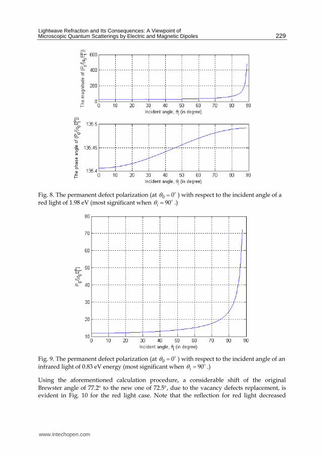
Fig. 8. The permanent defect polarization (at 0 0 ) with respect to the incident angle of a

red light of 1.98 eV (most significant when 90i .)

Fig. 9. The permanent defect polarization (at 0 0 ) with respect to the incident angle of an

infrared light of 0.83 eV energy (most significant when 90i .)

Using the aforementioned calculation procedure, a considerable shift of the original

Brewster angle of 77.2 to the new one of 72.5, due to the vacancy defects replacement, is evident in Fig. 10 for the red light case. Note that the reflection for red light decreased

www.intechopen.com


230

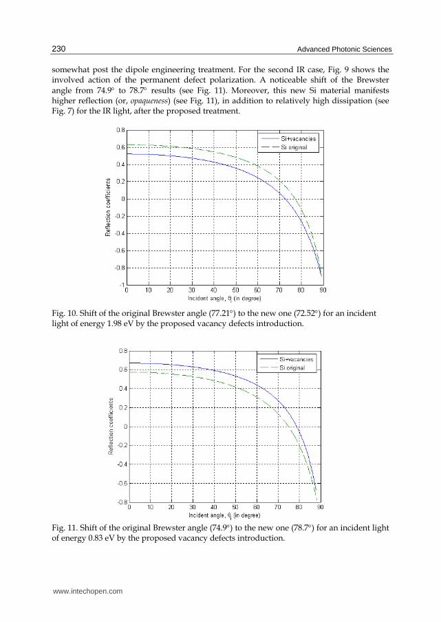
somewhat post the dipole engineering treatment. For the second IR case, Fig. 9 shows the involved action of the permanent defect polarization. A noticeable shift of the Brewster

angle from 74.9 to 78.7 results (see Fig. 11). Moreover, this new Si material manifests higher reflection (or, opaqueness) (see Fig. 11), in addition to relatively high dissipation (see Fig. 7) for the IR light, after the proposed treatment.

Fig. 10. Shift of the original Brewster angle (77.21) to the new one (72.52) for an incident light of energy 1.98 eV by the proposed vacancy defects introduction.

Fig. 11. Shift of the original Brewster angle (74.9) to the new one (78.7) for an incident light of energy 0.83 eV by the proposed vacancy defects introduction.

www.intechopen.com


231

In the above, the shifted Brewster angles for both cases are associated with considerable

dissipation caused by the introduced defects, as implied by Fig. 7. In particular, the defect-

modified silicon wafer would absorb the total power of the p-wave incident at the Brewster

angle. Nonetheless, this should not represent as sure characteristics for the general

situations. For example, a B -altering surface material (to be coated on the original host in a

post-process manner) may have its permanent polarization implemented via replacing some

of its atoms with other elements, instead of vacancies, and thus may not show such

dissipating behavior.

6. Poled PVDF films and asymmetric reflection experiments

6.1 Background on the PVDF material ((Pa llathadka, 2006), (Zhang et al., 2002)) and its preparations

Polyvinylidene difluoride, or PVDF (molecular formula: -(CH2CF2)n-), is a highly non-

reactive, pure thermoplastic and low-melting-point (170C) fluoropolymer. As a specialty plastic material in the fluoropolymer family, it is used generally in applications requiring the highest purity, strength, and resistance to solvents, acids, and bases. With a glass transition temperature (Tg) of about -35oC, it is typically 50-60% crystalline at room temperature. However, when stretched into thin film, it is known to manifest a large piezoelectric coefficient of about 6-7 pCN-1, about 10 times larger than those of most other polymers. To enable the material with piezoelectric properties, it is mechanically stretched and then poled with externally applied electric field so as to align the majority of molecular chains ((Pallathadka, 2006) , (Zhang et al., 2002)). These polarized PVDFs fall in 3 categories in general, i.e., alpha (TGTG'), beta (TTTT), and gamma (TTTGTTTG') phases, differentiated by how the chain conformations, of trans (T) and gauche (G), are grouped. FTIR (Fourier transform IR) measurements are normally employed for such differentiation purposes ((Pallathadka, 2006) , (Zhang et al., 2002)). With variable electric dipole contents (or, polarization densities) these PVDF films become ferroelectric polymers, exhibiting efficient piezoelectric and pyroelectric properties, making them versatile materials for sensor and battery applications.

In our experiments, PVDF films of Polysciences (of PA, USA) are subjected to non-uniform mechanical and electric polings to generate -PVDF films of distributed dipolar regions. By applying infrared light beams on these poled -PVDF films, the evidences of enhanced asymmetric refraction at varying incident angles as well as its inverse dependence on the incident power are sought for.

6.2 FTIR measurement setup

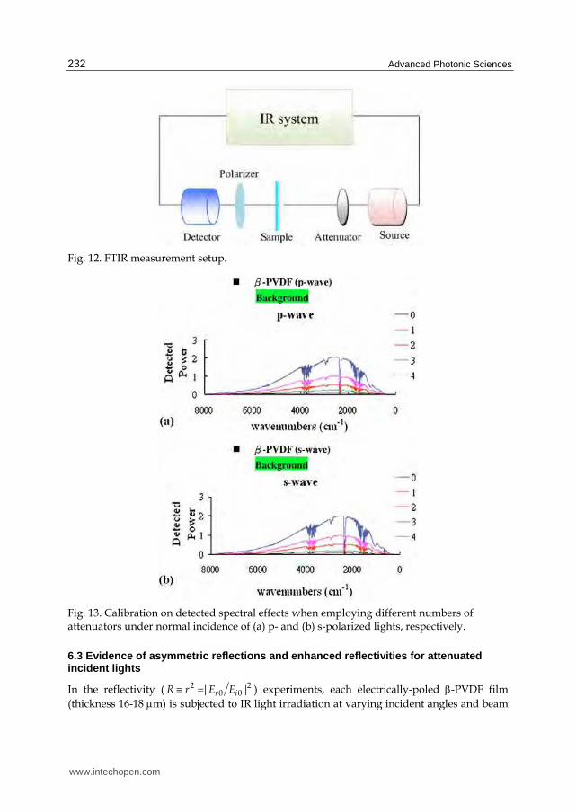
The adopted experimental setup takes full advantage of the original commercial FTIR measurement structure (Varian 2000 FT-IR) (Chen et al., 2008). The intended investigations are facilitated by putting an extra polarizer (Perkin-Elmer) in front of the detector and some predetermined number of optical attenuators (Varian) before the sample (see, Fig. 12). Figs. 13(a) and 13(b) show the detector calibration results under different numbers of attenuating sheets for both the p- and s-wave incidence, respectively. As is obvious, the detected intensities degraded linearly with the number of attenuators installed and the spectra remain morphologically similar.

www.intechopen.com


232

Fig. 12. FTIR measurement setup.

Fig. 13. Calibration on detected spectral effects when employing different numbers of attenuators under normal incidence of (a) p- and (b) s-polarized lights, respectively.

6.3 Evidence of asymmetric reflections and enhanced reflectivities for attenuated incident lights

In the reflectivity ( 2 20 0| |r iR r E E ) experiments, each electrically-poled -PVDF film

(thickness 16-18 m) is subjected to IR light irradiation at varying incident angles and beam

www.intechopen.com


233

intensities (via using the above attenuator films) (Chen et al., 2008). Even though a PVDF

film encompasses many double layers along its thickness, the reason the above theoretical

derivations based on a single double layer (see Fig. 5) should still apply is that there are non-

uniform vertical polarizations (or, electric fields) at the surface. In other words, the resultant

gradients in the incident-light-responsive planar dipole moment would then render nonzero

interfacial jump of ||E as addressed by Eq. (26).

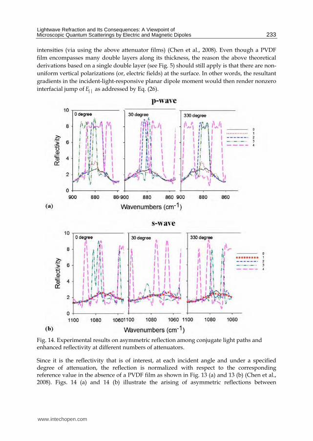
Fig. 14. Experimental results on asymmetric reflection among conjugate light paths and enhanced reflectivity at different numbers of attenuators.

Since it is the reflectivity that is of interest, at each incident angle and under a specified degree of attenuation, the reflection is normalized with respect to the corresponding reference value in the absence of a PVDF film as shown in Fig. 13 (a) and 13 (b) (Chen et al., 2008). Figs. 14 (a) and 14 (b) illustrate the arising of asymmetric reflections between

www.intechopen.com


234

conjugate incident paths (e.g., incidence at 30 versus 330) for both the p- and s-polarized infrared lights under various degrees of intended attenuation (Chen et al., 2008). In the above, the incident angle is defined by rotating clockwise the poled-PVDF sample under top-view of the setup of Fig. 12. Hence, reversing the light reflection path indeed causes a different reflected power to arise, as predicted by the aforementioned theoretical exploration. Note that, however, in traditional FTIR measurements, decrease in the detected intensity has been routinely attributed to increased absorption by PVDF films. Nevertheless, for an obliquely incident light the beam path within PVDF is only slightly larger than that in a normal incident situation. Thus, the resultant infinitesimal increase in PVDF absorption should never be sufficient to account for the detected large difference in reflected power. Notably, the detected decrease in intensity should instead be attributed to enhanced reflection caused by distributed dipoles on the poled PVDF films.

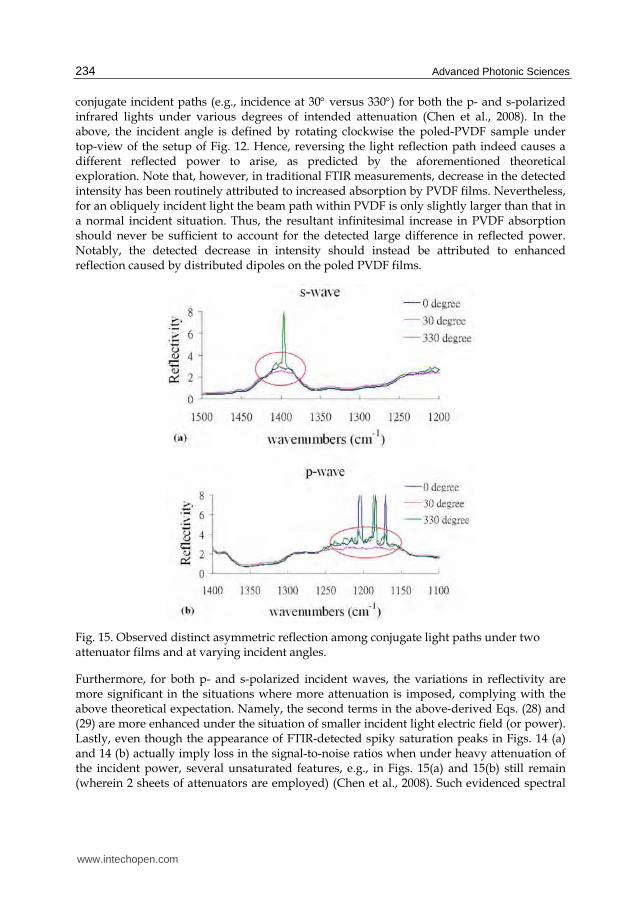
Fig. 15. Observed distinct asymmetric reflection among conjugate light paths under two attenuator films and at varying incident angles.

Furthermore, for both p- and s-polarized incident waves, the variations in reflectivity are more significant in the situations where more attenuation is imposed, complying with the above theoretical expectation. Namely, the second terms in the above-derived Eqs. (28) and (29) are more enhanced under the situation of smaller incident light electric field (or power). Lastly, even though the appearance of FTIR-detected spiky saturation peaks in Figs. 14 (a) and 14 (b) actually imply loss in the signal-to-noise ratios when under heavy attenuation of the incident power, several unsaturated features, e.g., in Figs. 15(a) and 15(b) still remain (wherein 2 sheets of attenuators are employed) (Chen et al., 2008). Such evidenced spectral

www.intechopen.com


235

features strongly endorse the above theoretical claim that the reflectivity variation of a dimmer light is more outstanding than that of a brighter one.

7. PVDF experiment on varying Brewster angle

7.1 PVDF new Brewster angle

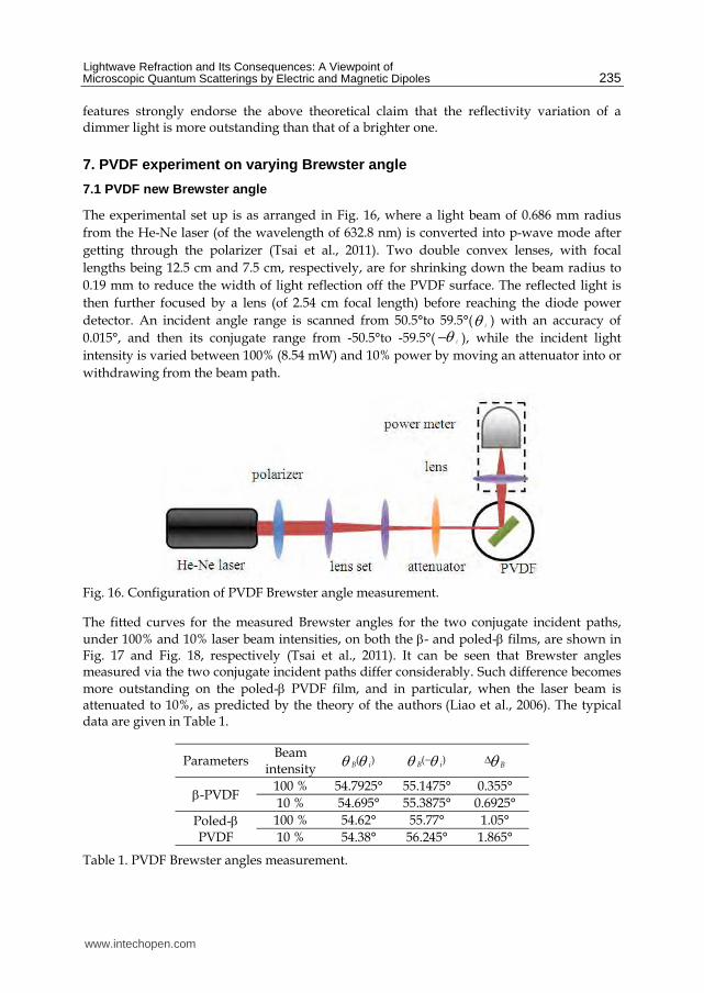
The experimental set up is as arranged in Fig. 16, where a light beam of 0.686 mm radius

from the He-Ne laser (of the wavelength of 632.8 nm) is converted into p-wave mode after

getting through the polarizer (Tsai et al., 2011). Two double convex lenses, with focal

lengths being 12.5 cm and 7.5 cm, respectively, are for shrinking down the beam radius to

0.19 mm to reduce the width of light reflection off the PVDF surface. The reflected light is

then further focused by a lens (of 2.54 cm focal length) before reaching the diode power

detector. An incident angle range is scanned from 50.5°to 59.5°( i ) with an accuracy of

0.015°, and then its conjugate range from -50.5°to -59.5°( i ), while the incident light

intensity is varied between 100% (8.54 mW) and 10% power by moving an attenuator into or

withdrawing from the beam path.

Fig. 16. Configuration of PVDF Brewster angle measurement.

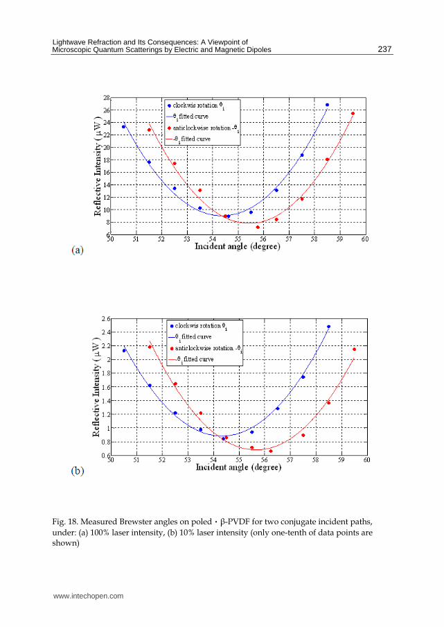
The fitted curves for the measured Brewster angles for the two conjugate incident paths,

under 100% and 10% laser beam intensities, on both the - and poled- films, are shown in Fig. 17 and Fig. 18, respectively (Tsai et al., 2011). It can be seen that Brewster angles measured via the two conjugate incident paths differ considerably. Such difference becomes

more outstanding on the poled- PVDF film, and in particular, when the laser beam is attenuated to 10%, as predicted by the theory of the authors (Liao et al., 2006). The typical data are given in Table 1.

Parameters Beam

intensity ( )

B i ( )B i

B

-PVDF 100 % 54.7925° 55.1475° 0.355°

10 % 54.695° 55.3875° 0.6925°

Poled- PVDF

100 % 54.62° 55.77° 1.05°

10 % 54.38° 56.245° 1.865°

Table 1. PVDF Brewster angles measurement.

www.intechopen.com


236

It is noted that although even the intrinsic phase PVDF possesses birefringence and this can lead to different Brewster angles as in the above too, the difference degree is at most around 0.129°, and hence may be ignored.

Fig. 17. Measured Brewster angles on・┚-PVDF for two conjugate incident paths, under: (a)

100% laser intensity, (b) 10% laser intensity (only one-tenth of data points are shown)

www.intechopen.com


237

Fig. 18. Measured Brewster angles on poled・┚-PVDF for two conjugate incident paths,

under: (a) 100% laser intensity, (b) 10% laser intensity (only one-tenth of data points are shown)

www.intechopen.com


238

This can be verified by putting into Eq. (23) the known ordinary and extraordinary refractive indices of PVDF and getting the Brewster angles of 54.814° and 54.933°,

respectively. Further, the fact that the larger deviation is evidenced in the poled- phase, as

compared with that from the phase, indicates that permanent dipoles are indeed the cause of such alteration in Brewster angles.

By putting the above experimental data (i.e., Table 1) into Eq. (23), the relative dielectric coefficients ( r ) for both the - and poled- PVDF films are extracted and tabulated in Table 2 (Tsai et al., 2011).

Parameters Beam

intensity ( )

r i ( )r i

-PVDF 100 % 2.008 1.994

10 % 2.062 2.1

Poled- PVDF

100 % 1.983 1.948

10 % 2.16 2.239

Table 2. Relative dielectric coefficients through fitting experimental data.

Then, the averaged effective permanent polarization 0P and orientation 0 can be extracted through trial-and-error (see, Table 3) by putting these coefficients into Eqs. (22) and (24), and using the relations:

p p

t iptE E and i t i2 cos cos cos

p

air air tt n n n . In the above, 0

p

iS CE , 1

isinsint air tn n , with S , 0 , and C being the irradiating light

intensity per unit area, the vacuum permittivity (i.e., 128.85 10 F/m), and the light speed in vacuum, respectively, and

2

r on (Tsai et al., 2011).

Parameters 0

0P

-PVDF 41.64° 9 21.0226 10 /C m

Poled- PVDF 61.62° 9 21.7843 10 /C m

Table 3. Extracted effective permanent polarizations and orientations of dipole-engineered PVDF films.

It can be seen that the electro-poling has caused the permanent polarization to increase somewhat, and most of all, its orientation with respect to the interface to add around 20°.

7.2 Novel 2D refractive index ellipse

Owing to its intrinsic uniaxial birefringence property ((Matsukawa et al., 2006), (Yassien et

al., 2010)), when a light is incident upon a PVDF film (as formed, without poling), the

www.intechopen.com


239

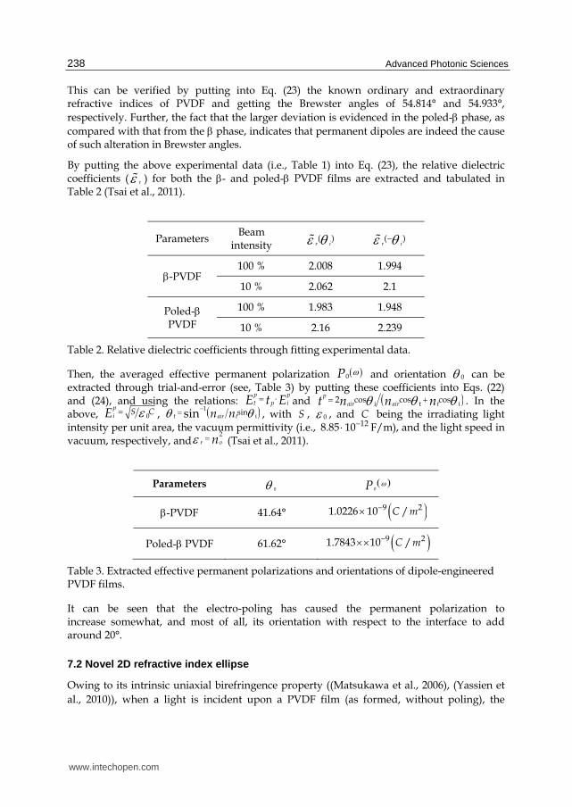
refracted light is decomposed into an ordinary wave and an extraordinary wave, which

correspond to refractive indices of no and ne , respectively. Namely, when the plane-of-

incident is formed by the light’s propagating direction vector k

and the uniaxis z (see, Fig.

19), with the angle between them being , then a slice on the 3D refractive index ellipsoid

cutting perpendicular to k

will give rise to an elliptic contour which is of the minor axis no

and major axis ns in a relationship expressed as:

n

sin

n

cos

n eos2

2

2

2

2

1 (30)

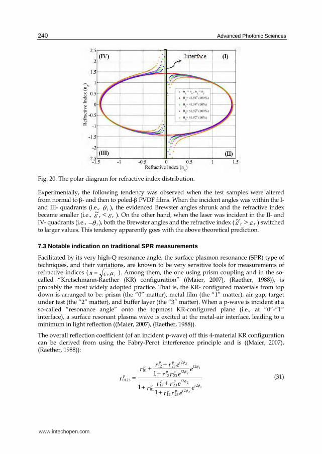
However, the whole picture will change considerably in the presence of ordered permanent

dipoles. Namely, unlike the traditional elliptic contour in red color in the polar diagram Fig.

20, unconventional contours in blue and green represent 2D (two dimension) refractive

index surfaces of the situation on -PVDF (i.e., 64.410 °) under 100 % and 10 % laser

power, respectively; and those in purple and orange colors are on poled- PVDF (i.e.,

62.610 °) under 100 % and 10 % laser power, respectively (Tsai et al., 2011). Note that, in

Fig. 20, as the ordinate dimension is along the direction of interface (in green) and the

abscissa along the norm in real setup, both the I and III quadrants describe the refraction in

the incident angle range of 0°~ 90° (i.e., i ), and quadrants II and IV depicts that of 0°~ -90°

(i.e., i ). Hence, the dipole-engineered ones would demonstrate open splittings near the

traditional incident angles. Among them, the deviation should be more outstanding for the

case with the test film being poled- than -PVDF, and especially when at lower incident

laser power (Tsai et al., 2011).

Fig. 19. Construction of the refractive index surface.

www.intechopen.com


240

Fig. 20. The polar diagram for refractive index distribution.

Experimentally, the following tendency was observed when the test samples were altered from normal to - and then to poled- PVDF films. When the incident angles was within the I- and III- quadrants (i.e., i ), the evidenced Brewster angles shrunk and the refractive index became smaller (i.e., rr ~ ). On the other hand, when the laser was incident in the II- and IV- quadrants (i.e., i ), both the Brewster angles and the refractive index ( rr ~ ) switched to larger values. This tendency apparently goes with the above theoretical prediction.

7.3 Notable indication on traditional SPR measurements

Facilitated by its very high-Q resonance angle, the surface plasmon resonance (SPR) type of techniques, and their variations, are known to be very sensitive tools for measurements of refractive indices ( rrn ). Among them, the one using prism coupling and in the so-called “Kretschmann-Raether (KR) configuration” ((Maier, 2007), (Raether, 1988)), is probably the most widely adopted practice. That is, the KR- configured materials from top down is arranged to be: prism (the “0” matter), metal film (the “1” matter), air gap, target under test (the “2” matter), and buffer layer (the “3” matter). When a p-wave is incident at a so-called “resonance angle” onto the topmost KR-configured plane (i.e., at “0”-“1” interface), a surface resonant plasma wave is excited at the metal-air interface, leading to a minimum in light reflection ((Maier, 2007), (Raether, 1988)).

The overall reflection coefficient (of an incident p-wave) off this 4-material KR configuration can be derived from using the Fabry-Perot interference principle and is ((Maier, 2007), (Raether, 1988)):

eerr

errr

eerr

errr

ri

ipp

ippp

iipp

ippp

p

1

2

2

1

2

2

22

2312

22312

01

22

2312

22312

01

0123

11

1

(31)

www.intechopen.com


241

And, the overall reflectivity in power is: rR p0123

2 , where r p01 , r p

12 , r p23 are reflection

coefficients at “0”-“1”, “1”-“2”, and “2”-“3” interfaces according to the traditional Fresnel

equations; and dcosk iiii 0 are phase angles associated with matters “1” and “2”,

respectively; and k0 is incident wave vector; and d11 and d 22 are relative dielectric

coefficient / layer thickness of the metal film and material under test, respectively.

However, it is found in the above experiments that in the presence of permanent dipoles,

not only is the Brewster angle dependent on the incident light power as well as the dipole

orientation, but also that two conjugate incident light paths result in distinctively different

refractions. Therefore, although the form of Eq. (31) remains the same in the presence of

permanent dipoles, values of local reflection coefficients involved can vary considerably

from those of their classical counterparts. In other words, the traditional confidence in SPR

type of measurements may be in jeopardy when the material under test is embedded with

permanent dipoles, as will be shown in what follows.

Consider a KR-configured SPR measurement setup as an example. It includes: a lens (SF 11)

of relative dielectric coefficient of 7786.1 2 , a silver metal film of 52 nm ( d1 ) thickness of a

relative dielectric coefficient of i67.06.17 (Raether, 1988), a PVDF film (as grown, or ,

or poled-) as the material under test of thickness of about 15 m ( d 2 ), with its original

relative dielectric coefficients being no2 and ne

2 , and a buffer layer of air of a relative

dielectric coefficient of about 1. This configuration is then subjected to the irradiation of a

light beam , from a 632.8 nm wavelength He-Ne laser, of the incident angles ranging within

50°~70°( i ) and its conjugate counterpart paths within the angle range -50°~ -70°( i ).

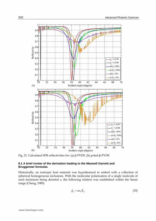
The numerical calculation result based on the above setup is shown in Fig. 21 and

indicates the following (Tsai et al., 2011). The birefringence (i.e., ne besides no ) of as-

grown PVDF suffices to give a maximal SPR resonance angle deviation of about 0.5°

(away from 58°). This deviation of resonance angles is considerably amplified in the -

(2.5°) and poled- (4°) cases, owing to the increase of permanent polarization density and

alignment. In such sensitive SPR type of measurements, these large deviations of

resonance angles represent large distortions in the light reflectivity, as illustrated in Fig.

21. Notably, it also affirms the theoretical prediction (see, Eq. (24)) that the reflectivity

coefficient is inversely proportional to the strength of the incident (or, transmitted) light

electric field. All these findings indicate that traditional SPR type of measurements needs

to exercise precaution when the material under test is embedded with permanent dipoles.

For example, most living cells are with cell walls made of two opposite double layers of

dipolar molecules (Alberts et al., 2007).

8. The quasistatic macroscopic mixing theory for magnetic permeability

Although mixing formulas for the effective-medium type of approximations for the

dielectric permittivities in the infinite-wavelength (i.e., quasistatic) limit (Lamb et al., 1980),

such as the Maxwell Garnett formula (Garnett, 1904), have been popularly applied in the

whole spectral range of electromagnetic fields, their magnetic counterpart has seldom been

addressed up to this day. The current effort is thus to derive such an equation to

approximately predict the final permeability as the result of mixing together several

magnetic materials (Chang & Liao, 2011).

www.intechopen.com


242

Fig. 21. Calculated SPR reflectivities for: (a) ┚-PVDF, (b) poled-┚-PVDF.

8.1 A brief review of the derivation leading to the Maxwell Garnett and Bruggeman formulas

Historically, an isotropic host material was hypothesized to embed with a collection of spherical homogeneous inclusions. With the molecular polarization of a single molecule of such inclusions being denoted α, the following relation was established within the linear range (Cheng, 1989):

0 m mp E (32)

www.intechopen.com


243

where mp

was the induced dipole moment and mE

was the polarizing electric field intensity

at the location of the molecule. Since the treatment was aiming for uniform spherical

inclusions, the polarizability became a scalar, such that mE

was expressed as (Purcell, 1985):

m p nearE E E E (33)

Here E

was the average field within the bulk host, pE

was the electric field at this

molecular location caused by all surrounding concentric spherical shells of the bulk, and

nearE

was due to asymmetry within the inclusion. In those cases of interest where either the

structure of the inclusion was regular enough, such as a cubical or spherical particulate, or

all incorporated molecules were randomly distributed, nearE

became essentially zero. It was

further approximated that 0/ 3mE E P (Purcell, 1985), to be elaborated later, with P

being the polarization density associated with a uniformly polarized sphere, and ε0 being

the permittivity in free space. Hence, given Eq. (32), with the number density of such

included molecules denoted as n, and mP np (Cheng, 1989), the polarization density was

further expressed as:

0 0/ 3 P n E P (34)

However, it was well-known that for isotropic media 01rP E where εr stood for the

relative permittivity (i.e., the electric field at the center of a uniformly polarized sphere (with

P

being its polarization density) was 0/ 3P ). Then, a relation known as the Lorentz-

Lorenz formula readily followed ((Lorenz, 1880), (Lorentz, 1880)):

3 1

2

r

rn (35)

In those special cases where the permittivity of each tiny included particle was εs and the host material was vacuum (εr =1), such that n = V-1 (V being the volume of the spherical inclusions), and Eq. (35) would have to satisfy (Garnett, 1904):

0

0

32

ss

V (36)

Combining Eqs. (35) and (36) gave the effective permittivity (εeff) of the final mixture (Garnett, 1904):

00 0 0

0 0

32

s

eff r

s s

ff

(37)

with f = nV being the volume ratio of the embedded tiny particles (0 ≤ f ≤ 1) within the final mixture. If, instead of vacuum, the host material was with a permittivity of εh, Eq. (37) was then generalized to the famous Maxwell Garnett mixing formula:

32

s h

eff h h

s h s h

ff

(38)

www.intechopen.com


244

For the view in which the inclusion was no longer treated as a perturbation to the original host material, Bruggeman managed to come up with a more elegant form wherein different ingredients were assumed to be embedded within a host (Bruggeman, 1935). By utilizing Eqs. (35) and (36), he had:

0 0

0 02 2

eff ii

ieff i

f (39)

where fi and εi are the volume ratio and permittivity of the i-th ingredient.

8.2 The magnetic flux density at the center of a uniformly magnetized sphere

surface current can be expected to appear on the surface of a uniformly magnetized sphere

(wherein M

is the finalized net anti-responsive magnetization vector, see Fig. 22).

Fig. 22. Situation for calculation of the central magnetic flux density on a uniformly magnetized sphere.

In Fig. 22,

SK is the induced anti-reactive surface current density (in A/m) on the sphere’s

surface. By integrating all surface current density on strips of the sphere’s surface the

magnetic flux density ( cB

) at the center of a uniformly magnetized sphere is obtained to be

(Lorrain & Corson, 1970):

02

3

c

MB (40)

8.3 Magnetic permeabilit ies formula mixing

Now, this time consider an isotropic host material embedded with a collection of spherical

homogeneous magnetic particles. Given the magnetic flux density at the location of a single

molecule of the inclusions being mB

, the following relation holds in general:

www.intechopen.com


245

m c nearB B B B (41)

where B

is the average magnetic flux density within the bulk host and nearB

is due to the

asymmetry in the inclusion. In those cases of interest where either the structure of the

included particles is regular enough, such as a cubical or spherical particulate, or all

incorporated molecules are randomly distributed, nearB

can be taken as zero.

If the magnetic field intensity at the location of the molecule is denoted mH

, the induced

magnetic dipole moment (mm) is:

m m mm H (42)

where m is the molecular magnetization of the molecule. Because M

equals mnm

, we have

(Cheng, 1989)

m m m mM n H H (43)

where m is known as the magnetic susceptibility. Hence, mB

can be further expressed as

(Cheng, 1989)

0 0 01 1 m r m m m m mB H n H H (44)

with μr being the relative permeability. By incorporating Eq. (41) and Eq. (44) into Eq. (43) we obtain:

0

0

2

1 3

m

m

n MM B

n (45)

Further, for isotropic magnetized materials (Cheng, 1989):

0

11 ,r

r

r

BM H

or

0

1

r

r

B M (46)

Substituting Eq. (46) into Eq. (45) gives (Chang & Liao, 2011)

3 1

2 5

rm

rn (47)

In the special case where the host material is vacuum (μr = 1) and the permeability of the spherical particles is μs, n = V-1 (V being the volume of a spherical particle), and Eq. (47) is satisfied by:

0

0

32 5

s

m

s

V (48)

www.intechopen.com


246

Combining Eqs. (47) and (48) gives the effective permeability (μeff) of the final mixture, i.e. (Chang & Liao, 2011),

00 0 0

0 0

32 5 2

eff r f

f (49)

Where f = nV is the volume ratio of the embedded particles within the mixture (0 ≤ f ≤ 1). In the more general situations where the host is no longer vacuum but of the permeability μh, then the more general mixing formula of permeabilities becomes (Chang & Liao, 2011):

32 5 2

s h

eff h h

s h s h

ff

(50)

As with Bruggeman’s approach for dielectrics (Bruggeman, 1935), the derived magnetic permeability formula can be generalized to the multi-component form (Chang & Liao, 2011):

0 0

0 02 5 2 5

eff ii

ieff i

f (51)

where fi and μi denote the volume ratios and permeabilities of the involved different inclusions, respectively. Or (Chang & Liao, 2011),

1 1

2 5 2 5

reff rii

ireff ri

f (52)

Although the actual mixing procedures can vary widely such that substantial deviations may result between the theoretical and measured values, Eq. (52) should still serve as a valuable guide when designing magnetic materials or composites.

9. A practical method to secure magnet ic permeability in optical regimes

As widely known, electronic polarization is involved in the absorption of electromagnetic wave within materials and this mechanism is represented by permittivity even in light-wave frequencies. However, refractive index which describes light absorption and reflection is calculated in terms of permittivity and permeability (accounting for magnetization). But permeability spectra in light frequencies are hardly available for most materials. In contrast with it, permeabilities for various materials are fairly well documented at microwave frequencies (see, for example, (Goldman, 1999) and (Jorgensen, 1995)). It is noted that more often than not an electronic permittivity spectrum (εr(ω)) is secured by measuring its corresponding refractive index (N(ω)) while bluntly assuming its relative permeability (μr) to be unity. Obviously, this approach is one-sided and inappropriate. In particular, as we are entering the nanotech era, many new possibilities should emerge and surprise us with their novel optical permeabilities, for example, the originally nonmagnetic manganese crystal can be made ferromagnetic once its lattice constant is varied (Hummel, 1985). In this section, a method is proposed such that reliable optical permeability values can be obtained numerically.

The magnetic permeability of a specific material emerges fundamentally from wavefunctions of its electrons. In the popular density functional theory (DFT) approach, the

www.intechopen.com


247

role of these electron wavefunctions is taken by the one-electron spinorbitals, called the

Kohn-Sham orbitals ( os ) (see, e.g., (Shankar, 1994) and (Atkins & Friedman, 1997)). A

spinorbital is a product of an orbital wavefunction and a spin wavefunction:

os o s (53)

where o is the orbital part, and s is the spin part of os .

In the density functional theory, these spinorbitals are solutions to the equation:

2

1i

n

osi

r r

, (54)

where r is the local charge probability density function. Then, the exact ground-state

electronic energy as well as other electronic properties of this n-electron system are known

to be unique functions of ┩ ((Shankar, 1994), (Atkins & Friedman, 1997)). Further, the overall

wavefunction satisfying the Pauli exclusion principle is often expressed in terms of the

Slater determinant ((Shankar, 1994), (Atkins & Friedman, 1997)) as:

1 2 3

1/2! det

ntotal os os os osr n r r r r , (55)

Hence, the primitive transition rate of a typical electronic excitation within a material of interest can now be expressed in terms of the Fermi’s golden rule ((Shankar, 1994), (Atkins & Friedman, 1997)) as:

20 01 0 0

,

f fi i

total os os os osf i

R C H E E , (56)

where H1 is the first order perturbation to the Hamiltonian of electrons caused by a light

wave propagating within; 0i

os (of 0i

osE ) and 0f

os (of 0f

osE ) are the electron states (energies)

before and after the perturbation (H1) takes place, respectively; ω is the radian frequency of

the propagating light wave; ħ is Planck constant divided by 2┨; and C is a proportional

constant. H1 in Eq. (56) can be expressed as (Shankar, 1994):

1

02

M

eH A P

mc

(57)

where 0A

is the vector potential of the injected light wave; MP

is the momentum operator of

electrons in the material of interest. MP

represents electrons’ straight-line motion which

constitute electronic polarization. Thus substituting Eq. (57) into Eq. (56) will result in Rtotal

proportional to the imaginary part of εr (i.e. εrI). At the same time (Shankar, 1994),

1

02

M

eH B

mc

(58)

where 0B

is the magnetic flux density of the injected light wave; M is the magnetic

moment operator of electrons in the material of interest. M represents electrons’ angular

www.intechopen.com


248

momentum which constitutes magnetization. Thus substituting Eq. (58) into Eq. (56) will

result in Rtotal proportional to the imaginary part of μr (i.e. μrI).

Because

0M sP (59)

Thus according to Eq. (57), the spin part of os and εrI are irrelative. But s contains

angular momentum and therefore must be involved in μrI. From Eq. (56) and Eq. (58), we

can obtain μrI as follows:

Applying a spin-orbit decomposition (see Eqs. (53) and (55)) on the kernel of the transition rate expression in Eq. (56) suggests the convenience of defining parameters as follows:

0 0 01 0 1 0 0f f fi i i

os os o s o s totalH H t ,

(60a)

0 1 0f i

o o oH t , (60b)

0 1 0f i

s s sH t , (60c)

where through explicit matrix operations, it can be shown that

total o st t t , (61)

As a result, Eq. (56) can be rewritten as:

0 00 0

, ,

f fi i

total os os os o s os os o sf i f i

R C t E E C t t E E R R , (62)

where

20 01 0 0

,

f fi i

o o o o o of i

R C H E E , (63)

20 01 0 0

,

f fi i

s s s s s sf i

R C H E E , (64)

with Co and Cs being constant coefficients.

As aforementioned, despite being termed “electronic transition rate” to account for the

lightwave absorption within a material, the primitive transition rate Rtotal is in essence a

series of delta functions situated at varying frequencies (or energies, see Eq. (56)), and thus

is too spikey to be real. In fact, this spikey nature results from our attempt to describe the

dynamics of multitudes of electrons by a limited number of Kohn-Sham orbitals. Therefore,

Rtotal ought to be “smoothed” prior to being converted to a realistic absorption spectrum.

Here, Gaussian functions are adopted to replace all delta functions. The smoothed Rtotal, Ro

and Rs are now denoted as R'total, R'o and R's, respectively, and thus from Eq. (62) we have:

www.intechopen.com


249

total o sR R R , (65)

It is a common practice in the first-principle quantum mechanical calculations (such as by the computer codes CASTEP and DMol3 ((Clark et al., 2005), (Delley, 1990)) that R'o is normally set equal to εrI simulated with the “spin polarized” option in these kind of codes turned off (as in the nonmagnetic case).

Substituting Eq. (58) into Eq. (64) gives R's. And then the product of R'o and R's, R'total, is proportional to μrI (the scaling factor is defined as CM). With μr being linear and causal, there is an exact one-to-one correspondence between its real and imaginary parts as prescribed by the Kramers-Kronig relation (see, e.g., (Landau & Lifshitz, 1960)). Thus, the real part of μr (i.e., μrR ) is readily available once μrI is numerically obtained. To make all this happen, the calculation of R's is now in order.

Within the formulation of R's spectrum (see its unsmoothed form in Eq. (64)), physical

quantities 0f

s , 0i

s , Esf0 and Esi0 would emerge from CASTEP or DMol3 ((Clark et al.,

2005), (Delley, 1990)) simulations by selecting the “spin polarized” option. In evaluating the

bracketed term in Eq. (64), we first have:

0 0 01 0 0 0

0 0

1

2 2f f fi i i

s s s s M s s s

et H B S B

mc , (66)

where M S ( S

being the spin angular momentum), with the gyromagnetic ratio

2

ge

mc and g = 2 (Shankar, 1994), such that 0 0 0 0

2 2x x y y z z

e eS B S B S B S B

mc mc

in

Cartesian coordinate. Further, it is known that the spin angular momentum around the z

axis (Sz) (i.e., eigenvectors of 0f

s and 0i

s possess only two possible eigenvalues: either

+ħ/2 (spin up) or -ħ/2 (spin down), with ħ being the Planck’s constant divided by 2┨. Hence,

the two possible states of 0f

s and 0i

s expressed on the eigenbasis of Sz are (Shankar,

1994):

Spin up: 1

0s , spin down: 0

1s , while the spin angular momenta Sx, Sy and Sz

are: 0 1 0 1 0

, ,1 0 0 0 12 2 2

x y z

iS S S

i

(Shankar, 1994).

Hence, the value of the bracketed term ts of Eq. (66) varies according to the four possible

combinations of 0f

s and 0i

s , namely:

1. 0f

s and 0i

s both spin up such that

0 0

0 0 0 02 2

f i

s s s x x y y z z

e et S B j m S B S B S B jm

mc mc

00 00

0 1 0 1 0 11 0

1 0 0 0 1 02 2 2 2 4

yx zz z

B ie B B eB t

imc mc

www.intechopen.com


250

2. 0f

s spin up, and 0i

s spin down such that 0 04

s x y xy

et B iB t

mc

.

3. 0f

s spin down, and 0i

s spin up such that *

0 04

s x y xy

et B iB t

mc

.

4. 0f

s and 0i

s both spin down such that 04

s z z

et B t

mc

.

It is obvious that the values of |ts|2 for cases 1 and 4 are identical, i.e., |tz|2 ≡ Tz; and those for cases 2 and 3 are the same and are |txy|2 ≡ Txy.

To simplify the R's calculation without loss of generality, the magnetic flux density vector of

a linearly polarized electromagnetic wave is oriented to parallel to the z axis, i.e., 0 0zB B

( 0 0 0x yB B ). As a result, only Tz is relevant in the R's calculation. Further, as implied by its

representation, Tz is invariant in value regardless of what the initial and final energy levels

(Esf0 and Esi0) are in a transition, so long as Fermi’s golden rule is satisfied. This property

greatly facilitates the calculation of R's, in that R's now simply becomes proportional to the

number of identical-spin transition electron pairs. Within each transition pair there is an

energy difference of ħω while being irradiated by a linearly polarized light of frequency ω.

In first-principle quantum mechanical simulation codes, such as the CASTEP and DMol3, a finite number of Esf0 and Esi0 are generated to approximate the transitions of a multitude of electrons within a material of interest. In other words, each output energy value actually stands for a narrow continuous band of states centered at this specific value. Therefore, to simulate more closely to the reality, all delta functions of Esf0 and Esi0 are replaced with Gaussian functions prior to being added up into continuous density spectra, for both the “all spin-up” (case 1) and “all spin-down” (case 4) states, respectively. Since the magnetic properties are manifested by unpaired spins, and on the same energy level a spin-up is neutralized by a spin-down (Pauli’s exclusion principle), the net spin density spectrum is thus settled by subtracting that of the spin-downs from that of the spin-ups.

With all inner work laid out, the detailed procedure for evaluating R's is outlined as follows:

1. Subtract the density spectrum of the spin-down states from that of the spin-ups to result in the net spin density spectrum. The positive part of it is the net spin-up density spectrum, and the absolute value of the other part is the net spin-down density spectrum.

2. Randomly sample the net spin-up density spectrum at each energy of interest and denote the sampled energy value Ei if it is lower than the Fermi level, otherwise, name it Ej.

3. Define Pi,j, as the product of ni and nj, where ni and nj are the density-of-states at Ei and Ej, respectively. Namely, Pi,j is proportional to the number densities associated with a transition pairs of net spin-up electrons linked by an energy difference of Ei,j ≡ (Ej - Ei).

4. Calculate Pi,j’s and Ei,j’s for each (Ei, Ej) pair to get the net spin-up Pi,j vs. Ei,j collection. 5. Obtain the Pi,j vs. Ei,j collection for the net spin-down states in a similar fashion. 6. Then, obtain the union of the Pi,j vs. Ei,j collection of the net spin-downs and that of the

net spin-ups to result in the total Pi,j-Ei,j collection. 7. Replace all Pi,j delta peaks by Gaussian functions to arrive at the desired continuous

spectrum of R's.

www.intechopen.com


251

As mentioned, in those cases where the “spin polarized” option in, e.g., CASTEP is turned off, the resultant εrI spectra actually gives R'o in Eq. (65). With both R's and R'o being revealed, the optical μr spectrum of interest can be secured within a proportional constant CM, and then the Kramers-Kronig relation. Finally, this universal constant CM is uncovered by comparing the erected μrI spectrum with existing data covering from low to lightwave frequencies (Lide & Frederikse, 1994).

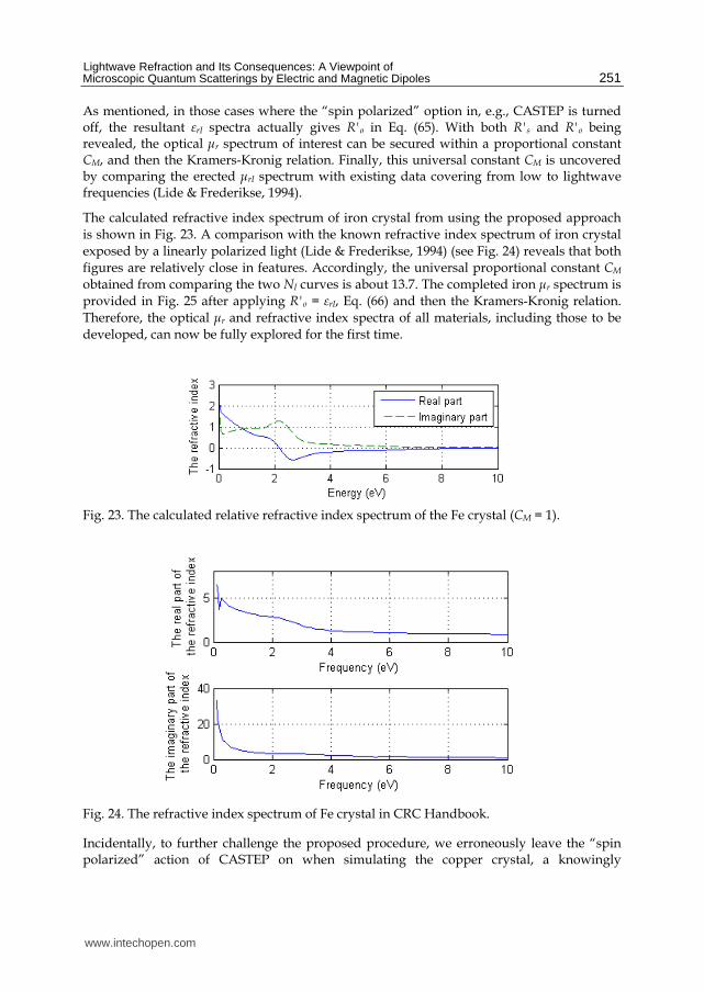
The calculated refractive index spectrum of iron crystal from using the proposed approach

is shown in Fig. 23. A comparison with the known refractive index spectrum of iron crystal

exposed by a linearly polarized light (Lide & Frederikse, 1994) (see Fig. 24) reveals that both

figures are relatively close in features. Accordingly, the universal proportional constant CM

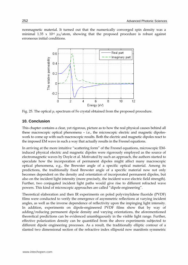
obtained from comparing the two NI curves is about 13.7. The completed iron μr spectrum is

provided in Fig. 25 after applying R'o = εrI, Eq. (66) and then the Kramers-Kronig relation.

Therefore, the optical μr and refractive index spectra of all materials, including those to be

developed, can now be fully explored for the first time.

Fig. 23. The calculated relative refractive index spectrum of the Fe crystal (CM = 1).

Fig. 24. The refractive index spectrum of Fe crystal in CRC Handbook.

Incidentally, to further challenge the proposed procedure, we erroneously leave the “spin polarized” action of CASTEP on when simulating the copper crystal, a knowingly

www.intechopen.com


252

nonmagnetic material. It turned out that the numerically converged spin density was a minimal 1.35 x 10-4 μB/atom, showing that the proposed procedure is robust against erroneous initial conditions.

Fig. 25. The optical μr spectrum of Fe crystal obtained from the proposed procedure.

10. Conclusion

This chapter contains a clear, yet rigorous, picture as to how the real physical causes behind all

these macroscopic optical phenomena – i.e., the microscopic electric and magnetic dipoles-

work to come up with such macroscopic results. Both the electric and magnetic dipoles react to

the imposed EM wave in such a way that actually results in the Fresnel equations.

In arriving at the more intuitive “scattering form” of the Fresnel equations, microscopic EM-induced physical electric and magnetic dipoles were rigorously employed as the source of electromagnetic waves by Doyle et al. Motivated by such an approach, the authors started to speculate how the incorporation of permanent dipoles might affect many macroscopic optical phenomena, e.g., the Brewster angle of a specific optical material. Among its predictions, the traditionally fixed Brewster angle of a specific material now not only becomes dependent on the density and orientation of incorporated permanent dipoles, but also on the incident light intensity (more precisely, the incident wave electric field strength). Further, two conjugated incident light paths would give rise to different refracted wave powers. This kind of microscopic approaches are called “dipole engineering”.

Theoretical elaboration and then IR experiments on poled polyvinylidene fluoride (PVDF) films were conducted to verify the emergence of asymmetric reflections at varying incident angles, as well as the inverse dependence of reflectivity upon the impinging light intensity. In addition, experiments on dipole-engineered PVDF films show that by way of adding/reducing permanent dipole density and varying orientations, the aforementioned theoretical predictions can be evidenced unambiguously in the visible light range. Further, effective polarization density can be quantified from the above experiments subjected to different dipole engineering processes. As a result, the traditionally elliptic contour of a slanted two dimensional section of the refractive index ellipsoid now manifests symmetric

www.intechopen.com


253

open splittings at near the traditional incident angle. It implies that severe challenge to the accuracy of traditional surface plasmon resonance measurements may arise in the presence of permanent dipoles of various morphologies, such as in the forms of nano-particles or membrane double layers.

Traditional approach of obtaining electric permittivity through directly measuring a material’s refractive index begins to appear flawed at dawn of the nanotech era. On the other hand, achieving novel magnetics and thus new materials of variable refractive indices starts to become meaningful. However, unlike its electric counterpart, data for optical magnetic permeability is hardly available for most materials. An effective method is proposed to secure practically accurate optical permeabilities through manipulating electronic transition rates generated by first-principle quantum mechanical simulations.

11. References

Alex J. Goldman. (1999). Handbook of Modern Ferromagnetic Materials, Springer, Kluwer Academic Publishers, Norwell, MA. (Goldman, 1999)

B. Alberts, A. Johnson, J. Lewis, M. Raff, K. Roberts. (2007). Molecular Biology of the Cell, Garland Science, New York. (Alberts et al., 2007)

B. Delley. (1990). "An allelectron numerical method for solving the local density functional

for polyatomic molecules", The Journal of Chemical Physics, vol. 92, (1990), 508. (Delley, 1990)

Chungpin Liao, Hsien-Ming Chang, and Chien-Jung Liao. (2006). “Manipulating the Brewster angles by using microscopically coherent dipole quanta and its possible implications,” IEEE Journal Lightwave Technology, vol. 24, no. 8, (Aug 2006), pp. 3248-3254. (Liao et al., 2006)

D. A. G. Bruggeman. (1935). „Berechnung verschiedener physi-kalischer Konstanten von heterogenen Substanzen. I. Di-elektrizitätskonstanten und Leitfähigkeiten der Mischkörper aus isotropen Substanzen“, Annalen der Physik, vol. 416, (1935), pp. 665-679. (Bruggeman, 1935)

D. R. Lide, H. P. R. Frederikse. (1994). CRC Handbook of Chemistry and Physics, pp.123-124, CRC-Press, Boca Raton, FL. (Lide & Frederikse, 1994)

David K. Cheng. (1989). Field and Wave Electromagnetics, second ed., Addison-Wesley Pub. Co., Reading, MA. (Cheng, 1989)

E. Hecht. (2002). Optics, 4th Ed., Addison Wesley, New York. (Hecht, 2002) Edward M. Purcell. (1985). Electricity and Magnetism, 2nd Ed., Education Development

Center, Inc., MA. (Purcell, 1985) Finn Jorgensen. (1995). The Complete Handbook of Magnetic Recording, McGraw-Hill, New

York. (Jorgensen, 1995) H. A. Haus and J. R. Melcher. (1989). Electromagnetic Fields and Energy, Prentice-Hall, New

York. (Haus & Melcher, 1989) H. A. Lorentz. (1880). „Ueber die Beziehung zwischen der Fortpflanzungsgeschwindigkeit

des Lichtes und der Körperdichte“, Annalen der Physik, vol. 9, (1880), pp. 641-665. (Lorentz, 1880)

H. Raether. (1988). “Surface Plasmons on Smooth and Rough Surfaces and on Gratings,” In: Springer Tracts in Modern Physics, Springer, Berlin. (Raether, 1988)

Hsien-Ming Chang and Chungpin Liao. (2011). "A Parallel Derivation to the Maxwell-Garnett Formula for the Magnetic Permeability of Mixed Materials", World Journal of Condensed Matter Physics, in press. (Chang & Liao, 2011)

www.intechopen.com


254

J. C. Maxwell Garnett. (1904). “Colours in Metal Glasses and in Metallic Films”, Philosophical Transactions of the Royal Society of London. Series A, Containing Papers of a Ma-thematical or Physical Character, vol. 203, (1904), pp. 385-420. (Garnett, 1904)

Jun-Lang Chen, Min-Yen Shieh, Hsin Her Yu, Chungpin Liao, Hsien-Ming Chang, Bin-Huang Yang, and Zi-Peng Zhao. (2008). "Asymmetric reflectivity from surfaces with distributed dipoles and IR experiments on poled polyvinylidene difluoride films", APPLIED PHYSICS LETTERS, vol. 93, 011902, (July 2008). (Chen et al., 2008)

K.M. Yassien, M. Agour, C. von Kopylow and H.M. EI-Dessouky. (2010). “On the digital holographic interferometry of fibrous material, I: Optical properties of polymer and optical fibers,” Optics and Lasers in Engineering , Vol. 48, Issue 5, (2010), pp. 555-560. (Yassien et al., 2010)

L. Lorenz. (1880). „Ueber die Refractionsconstante“, Annalen der Physik, Vol. 11, (1880), pp. 70-103. (Lorenz, 1880)

L.D. Landau, E.M. Lifshitz. (1960). Electrodynamics of Continuous Media, pp. 260-263, Pergamon Press, Oxford. (Landau & Lifshitz, 1960)

M. Matsukawa, K. Shintani, S. Tomohiro and N. Ohtori. (2006). “Application of Brillouin scattering to the local anisotropy and birefringence measurements of thin layers,” Ultrasonics, Vol.44, Suppl. 1, (2006), pp. e1555-e1559. (Matsukawa et al., 2006)

P. W. Atkins and R. S. Friedman. (1997). Molecular quantum mechanics, Oxford University Press, New York. (Atkins & Friedman, 1997)

Paul Lorrain, Dale R. Corson. (1970). Electromagnetic Fields and Waves, second ed., W.H.Freeman & Co Ltd, San Francisco. (Lorrain & Corson, 1970)

Po-Yu Tsai, Chien-Jung Liao, Wen-Kai Kuo, Chungpin Liao. (2011). "Birefringence caused by the presence of permanent dipoles and its possible threat on the accuracy of traditional surface plasmon", World Journal of Condensed Matter Physics, in press. (Tsai et al., 2011)

Pramoda K. Pallathadka. (2006). “Solid state 19F NMR study of crystal transformation in PVDF and its nanocomposites (polyvinylidene fluoride)”, Polymer Engineering and Science, 46(12), 1684-7, (2006). (Pallathadka, 2006)

Q. M. Zhang, V. Bharti, G. Kavarnos. (2002). "Poly (Vinylidene Fluoride) (PVDF) and its Copolymers", In: Encyclopedia of Smart Materials, M. Schwartz (Ed.), Volumes 1-2, pp. 807-825, John Wiley & Sons, and references therein. (Zhang et al., 2002)

R. Shankar. (1994). Principles of Quantum Mechanics, Springer Science & Business Media, New York. (Shankar, 1994)

Rolf E. Hummel. (1985). Electronic Properties of Materials, pp. 243-247, Springer-Verlag, New York. (Hummel, 1985)

S. A. Maier. (2007). Plasmonics: Fundamental and Applications, Springer, New York. (Maier, 2007) Stewart J. Clark, M.D. Segall, Christopher J Pickard, P.J. Hasnip, M. I. J. Probert, Keith

Refson, and Mike C. Payne. (2005). "First principles methods using CASTEP", Zeitschrift Fuer Kristallographie, vol. 220, (2005), pp. 567-570. (Clark et al., 2005)

W. Lamb, D. M. Wood, and N. W. Ashcroft. (1980). “Long-wavelength electromagnetic propagation in heterogeneous media”, Physical Review B, vol. 21, no. 6, (March 1980), pp. 2248-2266. (Lamb et al., 1980)

W. T. Doyle. (1985). “Scattering approach to Fresnel’s equations and Brewster’s law,” Am. J. Phys., 53 (5), pp. 463-468. (Doyle, 1985)

www.intechopen.com

Advanced Photonic SciencesEdited by Dr. Mohamed Fadhali

ISBN 978-953-51-0153-6Hard cover, 374 pagesPublisher InTechPublished online 21, March, 2012Published in print edition March, 2012

InTech EuropeUniversity Campus STeP Ri Slavka Krautzeka 83/A 51000 Rijeka, Croatia Phone: +385 (51) 770 447 Fax: +385 (51) 686 166www.intechopen.com

InTech ChinaUnit 405, Office Block, Hotel Equatorial Shanghai No.65, Yan An Road (West), Shanghai, 200040, China

Phone: +86-21-62489820 Fax: +86-21-62489821

The new emerging field of photonics has significantly attracted the interest of many societies, professionalsand researchers around the world. The great importance of this field is due to its applicability and possibleutilization in almost all scientific and industrial areas. This book presents some advanced research topics inphotonics. It consists of 16 chapters organized into three sections: Integrated Photonics, Photonic Materialsand Photonic Applications. It can be said that this book is a good contribution for paving the way for furtherinnovations in photonic technology. The chapters have been written and reviewed by well-experiencedresearchers in their fields. In their contributions they demonstrated the most profound knowledge andexpertise for interested individuals in this expanding field. The book will be a good reference for experiencedprofessionals, academics and researchers as well as young researchers only starting their carrier in this field.

How to referenceIn order to correctly reference this scholarly work, feel free to copy and paste the following:

Chungpin Liao, Hsien-Ming Chang, Chien-Jung Liao, Jun-Lang Chen and Po-Yu Tsai (2012). LightwaveRefraction and Its Consequences: A Viewpoint of Microscopic Quantum Scatterings by Electric and MagneticDipoles, Advanced Photonic Sciences, Dr. Mohamed Fadhali (Ed.), ISBN: 978-953-51-0153-6, InTech,Available from: http://www.intechopen.com/books/advanced-photonic-sciences/lightwave-refraction-and-its-consequences-a-viewpoint-microscopic-quantum-scatterings-by-electric-an

lightwave refraction and its consequences: a viewpoint of...

Documents