light water reactor sustainability program a simple ... iic system technologies/simple... · a...
TRANSCRIPT

INL/EXT-15-34729
Light Water Reactor Sustainability
Program
A Simple Demonstration of Concrete
Structural Health Monitoring
Framework
March 2015
U.S. Department of Energy
Office of Nuclear Energy

DISCLAIMER
This information was prepared as an account of work sponsored by an
agency of the U.S. Government. Neither the U.S. Government nor any
agency thereof, nor any of their employees, makes any warranty, expressed
or implied, or assumes any legal liability or responsibility for the accuracy,
completeness, or usefulness, of any information, apparatus, product, or
process disclosed, or represents that its use would not infringe privately
owned rights. References herein to any specific commercial product,
process, or service by trade name, trade mark, manufacturer, or otherwise,
does not necessarily constitute or imply its endorsement, recommendation,
or favoring by the U.S. Government or any agency thereof. The views and
opinions of authors expressed herein do not necessarily state or reflect
those of the U.S. Government or any agency thereof.

INL/EXT-15-34729 Revision 0
A Simple Demonstration of Concrete Structural Health Monitoring Framework
Sankaran Mahadevan, Vivek Agarwal, Guowei Cai, Paromita Nath, Yanqing Bao,
Jose Maria Bru Brea, Noah Myrent, David Koester, Douglas Adams, David Kosson
March 2015
Idaho National Laboratory Idaho Falls, Idaho 83415
http://www.inl.gov
Prepared for the
U.S. Department of Energy Office of Nuclear Energy
Under DOE Idaho Operations Office Contract DE-AC07-05ID14517

(This page intentionally left blank)


v
ABSTRACT
Assessment and management of aging concrete structures in nuclear power
plants require a more systematic approach than simple reliance on existing code
margins of safety. Structural health monitoring of concrete structures aims to
understand the current health condition of a structure based on heterogeneous
measurements to produce high-confidence actionable information regarding
structural integrity that supports operational and maintenance decisions.
This ongoing research project is seeking to develop a probabilistic
framework for health diagnosis and prognosis of aging concrete structures in a
nuclear power plant that is subjected to physical, chemical, environment, and
mechanical degradation. The proposed framework consists of four elements:
damage modeling, monitoring, data analytics, and uncertainty quantification.
This report describes a proof-of-concept example on a small concrete slab
subjected to a freeze-thaw experiment that explores techniques in each of the four
elements of the framework and their integration. An experimental set-up at
Vanderbilt University’s Laboratory for Systems Integrity and Reliability is used
to research effective combinations of full-field techniques, which include infrared
thermography, digital image correlation, and ultrasonic measurement. The
measured data are linked to the probabilistic framework. The thermography,
digital image correlation data, and ultrasonic measurement data are used for
Bayesian calibration of model parameters, diagnosis of damage, and prognosis of
future damage. The proof-of-concept demonstration presented in this report
highlights the significance of each element of the framework and their
integration.

vi
(This page intentionally left blank)

vii

viii
EXECUTIVE SUMMARY
One challenge for the current fleet of light water reactors in the United States is age-related
degradation of their passive assets that include concrete, cables, piping, and reactor pressure vessel. As
the current fleet of nuclear power plants (NPPs) continue to operate up to 60 years or beyond, it is
important to understand the current and the future health condition of passive assets under different
operating conditions that would support operational and maintenance decisions. To ensure long-term safe
and reliable operation of the current fleet, the U.S. Department of Energy’s Office of Nuclear Energy
funds the Light Water Reactor Sustainability (LWRS) Program to develop the scientific basis for
extending the operation of commercial light water reactors beyond the current license extension period.
The LWRS Program has three pathways. The online monitoring research of assets in nuclear power plants
is within the scope of research activities performed within the Advanced Instrumentation, Information,
and Control Systems Technologies Pathway. This effort also leverages the research performed within the
Material Aging and Degradation Pathway.
Among different passive assets of interest, concrete structures are investigated in this research project.
Reinforced concrete structures found in NPPs can be grouped into four categories: primary containment,
containment internal structures, secondary containments/reactor buildings, and spent fuel pool and
cooling towers. These concrete structures are affected by a variety of degradation mechanisms, related to
chemical, physical, and mechanical causes, and irradiation. The age-related degradation of concrete
results in gradual microstructural changes (slow hydration, crystallization of amorphous constituents,
reactions between cement paste and aggregates, etc.). Changes over long periods of time must be
measured, monitored, and analyzed to best support long-term operation and maintenance decisions.
Structural health monitoring (SHM) of concrete structures aims to understand the current health
condition of a structure based on heterogeneous measurements to produce high-confidence actionable
information regarding structural integrity and reliability. To achieve this research objective, Vanderbilt
University, in collaboration with Idaho National Laboratory (INL) and Oak Ridge National Laboratory
(ORNL) has proposed a probabilistic framework of research activities for the health monitoring of NPP
concrete structures subject to physical, chemical, and mechanical degradation. A systematic approach
proposed to assess and manage aging concrete structures requires an integrated framework that includes
the following four elements: damage modeling, monitoring, data analytics, and uncertainty quantification.
After proposing the above framework, a 2-day workshop was organized at Vanderbilt University in
November 2014 to identify the research gaps and opportunities for advancing the state-of-the-art in
concrete structures health management. Subsequently, researchers at Vanderbilt University and INL
developed a proof-of-concept example, using a small concrete slab and an aggressive freeze-thaw cycling,
that explores techniques in each of the four elements of the framework and their integration. Effective
combinations of full-field monitoring techniques, and related data analytics, structural modeling, and
diagnosis/prognosis techniques need to be identified for different types of concrete structures under
different loading and operating conditions. An experimental set-up at Vanderbilt University’s Laboratory
for Systems Integrity and Reliability is used to demonstrate the framework using infrared thermography,
digital image correlation (DIC), and ultrasonic measurement. The measured data are linked to a
probabilistic framework; the monitoring data is input to the Bayesian network for Bayesian calibration of
the model parameters, and for uncertainty quantification of diagnosis and prognosis results.
Some of the outcomes of this proof-of-concept demonstration example included:
1. The experiment and the analyses were conducted in four stages: intact slab, slab with drilled holes,
slab with holes subjected to freeze-thaw Cycle 1, and slab with holes subjected to freeze-thaw
Cycle 2.

ix
2. Finite element analysis (FEA) was used for prognosis, and its parameters were calibrated using
monitoring data. Four types of FEA models were developed, corresponding to the four stages of the
experiment mentioned above.
3. The FEA models were used to develop Gaussian process surrogate models to reduce the
computational effort in Bayesian calibration of model parameters using monitoring data, in Step 5
below.
4. Strain observations from DIC, and temperature observations from infrared thermography were used to
calibrate the finite element model parameters in the first two stages. Thermography images and
ultrasonic measurements in Stages 3 and 4 were used to inform the diagnosis and prognosis.
5. All modeling, experimental, and data analytics results were integrated using a Bayesian network, to
systematically quantify the uncertainty in model calibration, diagnosis, and prognosis. Quantifying
the uncertainty in diagnosis and prognosis is valuable for decision-making.
The methodologies described in this milestone report are focused on concrete SHM measurements,
data analytics, and development of uncertainty-quantified diagnostic and prognostics models that will
support continuous assessment of concrete performance. The proof-of-concept demonstration presented in
this report highlights the significance of each element of the framework and their integration.
In the next phase of the research, modeling of Alkali-Silica Reaction (ASR) degradation will be
developed using the Multiphysics Object Oriented Simulation Environment (MOOSE). The MOOSE
implementation would guide research in identifying and refining appropriate full-field monitoring
techniques. Vanderbilt University will collect and analyze data using a concrete slab with induced ASR
degradation, and advance the uncertainty quantification approaches and the integration framework. The
resulting comprehensive approach will facilitate the development of a quantitative, risk-informed
framework that would be generalizable for a variety of concrete structures.

x
ACKNOWLEDGMENTS
This report was made possible through funding by the U.S. Department of
Energy (DOE) Light Water Reactor Sustainability (LWRS) Program. We are
grateful to Richard Reister of DOE, and Bruce Hallbert and Kathryn McCarthy at
Idaho National Laboratory (INL) for championing this effort.

xi
(This page intentionally left blank)
xii
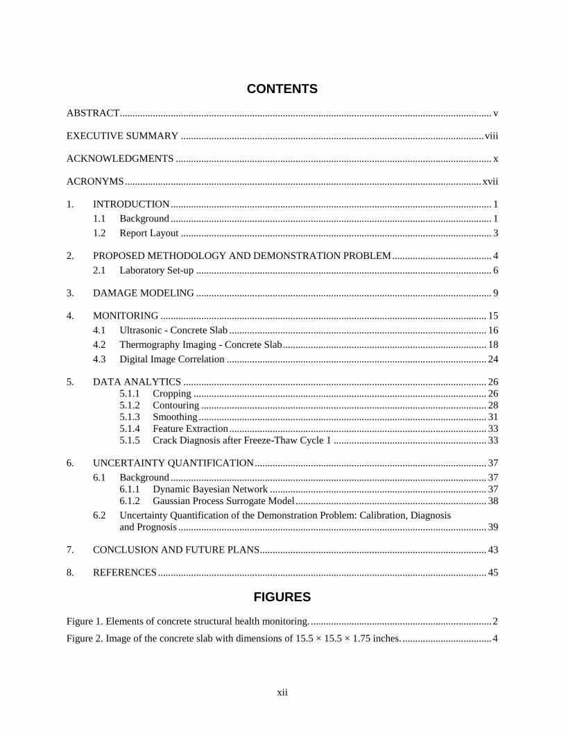
CONTENTS
ABSTRACT .................................................................................................................................................. v
EXECUTIVE SUMMARY ....................................................................................................................... viii
ACKNOWLEDGMENTS ............................................................................................................................ x
ACRONYMS ............................................................................................................................................ xvii
1. INTRODUCTION .............................................................................................................................. 1
1.1 Background .............................................................................................................................. 1
1.2 Report Layout .......................................................................................................................... 3
2. PROPOSED METHODOLOGY AND DEMONSTRATION PROBLEM ....................................... 4
2.1 Laboratory Set-up .................................................................................................................... 6
3. DAMAGE MODELING .................................................................................................................... 9
4. MONITORING ................................................................................................................................ 15
4.1 Ultrasonic - Concrete Slab ..................................................................................................... 16
4.2 Thermography Imaging - Concrete Slab ................................................................................ 18
4.3 Digital Image Correlation ...................................................................................................... 24
5. DATA ANALYTICS ....................................................................................................................... 26 5.1.1 Cropping ................................................................................................................... 26 5.1.2 Contouring ................................................................................................................ 28 5.1.3 Smoothing ................................................................................................................. 31 5.1.4 Feature Extraction ..................................................................................................... 33 5.1.5 Crack Diagnosis after Freeze-Thaw Cycle 1 ............................................................ 33
6. UNCERTAINTY QUANTIFICATION ........................................................................................... 37
6.1 Background ............................................................................................................................ 37 6.1.1 Dynamic Bayesian Network ..................................................................................... 37 6.1.2 Gaussian Process Surrogate Model ........................................................................... 38
6.2 Uncertainty Quantification of the Demonstration Problem: Calibration, Diagnosis
and Prognosis ......................................................................................................................... 39
7. CONCLUSION AND FUTURE PLANS ......................................................................................... 43
8. REFERENCES ................................................................................................................................. 45
FIGURES
Figure 1. Elements of concrete structural health monitoring. ....................................................................... 2
Figure 2. Image of the concrete slab with dimensions of 15.5 × 15.5 × 1.75 inches. ................................... 4

xiii
Figure 3. Image of the concrete slab with dimensions of 15.5 × 15.5 × 1.75 inches constrained
with a steel frame. ......................................................................................................................... 5
Figure 4. Temperature profile used to apply heat to the slab. ....................................................................... 5
Figure 5. A schematic representation of holes drilled into the side of the concrete slab. ............................. 6
Figure 6. Crack produced by the freeze-thaw cycles. ................................................................................... 6
Figure 7. Experimental set-up in the Laboratory for Systems Integrity and Reliability at
Vanderbilt University. (Left) Concrete slab with holes along with the ultrasonic
measurement unit. (Right) Concrete slab with thermography imaging and DIC
measuring units. ............................................................................................................................ 7
Figure 8. Location of the two thermocouples used to control the thermal blanket. ...................................... 7
Figure 9. Flow chart showing the connections of the measured data to the four elements of the
PHM framework. .......................................................................................................................... 8
Figure 10 Model configuration in Abaqus for slabs (a) intact and (b) damaged. ......................................... 9
Figure 11. Heat applied at one surface of the slab FEA model. (a) Intact slab, (b) slab with holes. .......... 10
Figure 12. Finite element mesh for (a) intact slab and (b) slab with holes. ................................................ 10
Figure 13. Temperature contours for (a) intact slab and (b) slab with holes. ............................................. 11
Figure 14. Strain contours for (a) intact slab, and (b) slab with holes. ....................................................... 11
Figure 15. Plot of (a) temperature and (b) maximum principal strain against thermal conductivity
k1. ................................................................................................................................................ 12
Figure 16. Plot of (a) temperature and (b) maximum principal strain against coefficient of thermal
convection k2. ............................................................................................................................. 13
Figure 17. (a) Cracked regions after diagnosis. (b) Predicted crack locations at section cut at
center of the slab. ........................................................................................................................ 14
Figure 18. Locations where the ultrasonic probe was placed. .................................................................... 16
Figure 19. Cross section of the 0.5-inch-diameter hole. ............................................................................. 17
Figure 20. Ultrasonic signal at Location 1. ................................................................................................. 17
Figure 21. Thermographic images of the healthy slab and damaged slab measured at a specific
time during the thermal cycle, damage areas are identified with arrows. ................................... 20
Figure 22. Thermographic results with and without the frame on slab....................................................... 24
Figure 23. Strain images of the healthy slab and damaged slab measured at the end of the thermal
cycle. ........................................................................................................................................... 26
Figure 24. Original image (left) and cropped image (right) at time 20 minutes. ........................................ 27
Figure 25. Contour of intact slab (left) and filled contour of intact slab (right) at 20 minutes. .................. 29
Figure 26. Contour of the slab with drilled holes (left) and filled contour of slab with drilled holes
(right) at 20 minutes. .................................................................................................................. 30
Figure 27. Extracted feature without smoothing (left) and extracted feature after smoothing
(right); the white spots shown on the right image are the suspected damage areas at
20 minutes................................................................................................................................... 32

xiv
Figure 28. Feature extracted for the slab with drilled holes, with frame (left), and without frame
(right), at 20 minutes. ................................................................................................................. 34
Figure 29. Feature extracted for the slab with the holes, at 18 min (left) and 40 min (right) ..................... 35
Figure 30. Diagnosis of slab with holes, before freeze-thaw Cycle 1 (left), and after freeze-thaw
Cycle 1 (right), at 20 minutes. .................................................................................................... 36
Figure 31. Bayesian Network illustration. .................................................................................................. 37
Figure 32. Gaussian process surrogate model example. ............................................................................. 39
Figure 33. Dynamic Bayesian Network. ..................................................................................................... 40
Figure 34. GP surrogate model for healthy slab (a) and damaged slab (b), ( ) vs . ......................... 41
Figure 35. Prior and posterior of and , updated by temperature and strain at t=0 and t=1,
respectively. ................................................................................................................................ 41
TABLES
Table 1. Material properties. ......................................................................................................................... 9
Table 2. Finite element mesh information. ................................................................................................. 10
Table 3. Ultrasonic measurement of the holes’ depth. ................................................................................ 18
Table 4. Mean and standard deviation. ....................................................................................................... 41

xv
(This page intentionally left blank)

xvi

xvii
ACRONYMS
ASR Alkali-Silica Reaction
BN Bayesian Network
DBN Dynamic Bayesian Network
DIC Digital Image Correlation
DOE Department of Energy
FEA Finite Element Analysis
GP Gaussian Process
IR Infra-red
INL Idaho National Laboratory
LASIR Laboratory for Systems Integrity and Reliability
LWRS Light Water Reactor Sustainability
MCMC Markov chain Monte Carlo
MOOSE Multiphysics Object-Oriented Simulation Environment
NDE Non-Destructive Evaluation
NIST National Institute of Standards and Technology
NPP Nuclear Power Plant
ORNL Oak Ridge National Laboratory
PHM Prognostics and Health Management
SHM Structural Health Monitoring

xviii
(This page intentionally left blank)

1
1. INTRODUCTION
As many existing nuclear power plants (NPPs) continue to operate beyond their license life, plant
structures, systems, and components suffer deterioration that affects their structural integrity and
performance. Health monitoring is an essential technology for insuring that the current and future state of
a NPP will meet performance and safety requirements. This project focuses on concrete structures in
NPPs. The concrete structures are grouped into four categories: primary containment, containment
internal structures, secondary containment/reactor buildings, and other structures such as used fuel pools,
dry storage casks, and cooling towers. These concrete structures are affected by a variety of chemical,
physical, and mechanical degradation mechanisms such as alkali-silica reaction (ASR), chloride
penetration, sulfate attack, carbonation, freeze-thaw cycles, shrinkage, and mechanical loading
(Naus, 2007). The age-related deterioration of concrete results in continuing microstructural changes
(slow hydration, crystallization of amorphous constituents, reactions between cement paste and
aggregates, etc.). Therefore, it is important that changes over long periods of time are measured,
monitored, and analyzed to best support long-term operation and maintenance decisions.
Structural health monitoring (SHM) is required to produce actionable information regarding structural
integrity that when conveyed to the decision-maker enables risk management with respect to structural
integrity and performance. The methods and technologies employed include the assessment of the critical
measurements, monitoring, and the analysis of aging concrete structures under different operating
conditions. In addition to the specific system being monitored, information may also be available for
similar or nominally identical systems in a fleet, as well as legacy systems. Therefore, Christensen (1990)
suggested that assessment and management of the aging concrete structures in NPPs require a more
systematic approach than simple reliance on existing code margins of safety.
Through the Light Water Reactor Sustainability (LWRS) Program, several national laboratories, and
Vanderbilt University have begun the concrete SHM research and development as per the proposed
framework discussed in the following section. The goal of this research is to enable plant operators to
make risk-informed decisions on structural integrity, remaining useful life, and performance of concrete
structures across the nuclear fleet. The long-term research objective of this project is to produce
actionable information regarding structural integrity that supports operational and maintenance decision
making, which is individualized for a given structure and its performance goals. In addition, the project
supports the research objectives of all three pathways under the LWRS Program.
This report presents a demonstration example performed at Vanderbilt University utilizing the
full-field techniques to assess the degradation in a small concrete slab. The demonstration example
showcases the effectiveness of the proposed concrete SHM framework. The summary of initial research
findings and future research activities are also presented in this report.
1.1 Background
Vanderbilt University, in collaboration with Idaho National Laboratory (INL) and Oak Ridge
National Laboratory (ORNL) personnel, proposed a framework for health diagnosis and prognosis of
aging concrete structures in NPPs subject to physical, chemical, and mechanical degradation
(Mahadevan et al., 2014 and Agarwal and Mahadevan, 2014). The proposed framework (as shown in
Figure 1) will investigate for the health of NPP concrete structures by integrating four technical elements:
(1) Damage modeling, (2) Monitoring, (3) Data analytics, and (4) Uncertainty quantification. For details
on each element of the proposed framework, refer Mahadevan et al. (2014). The framework will enable
plant operators to make risk-informed decisions on the structural integrity, remaining useful life, and
performance of concrete structures.

2
Figure 1. Elements of concrete structural health monitoring.
Damage Modeling: This element leverages the modeling of chemical, physical and mechanical
degradation mechanisms (such as alkali-aggregate reaction, chloride penetration, sulfate attack,
carbonation, freeze-thaw cycles, shrinkage, and radiation damage) in order to assist monitoring and risk
management decisions. Alkali-aggregate reaction is currently receiving prominent attention; however,
other appropriate damage mechanisms for NPP concrete structures can also be included. The interactions
of multiple mechanisms need significant consideration. The task requires modeling and computational
advances and combined-physics experiments, and the integration of multiple models through an
appropriate simulation framework.
Monitoring: This element explores effective combination of promising SHM techniques for full-field
multi-physics monitoring of concrete structures. Optical, thermal, acoustic, and radiation-based
techniques will be investigated for full-field imaging. Examples of these techniques include digital image
correlation (DIC), infrared imaging, velocimetry and ultrasonic, and X-ray tomography. A particular
consideration is the linkage of chemical degradation mechanisms to the observed degradation, which
requires synergy between the damage modeling and monitoring research.
Data analytics: The information gathered from multiple health monitoring techniques results in high
volume, rate, and variety (heterogeneity) of data. This element leverages big data techniques to store,
process, and analyze heterogeneous data (numerical, text and image) and arrive at effective inference of
concrete degradation. The data analytics framework can also integrate information from model prediction,
laboratory experiments, plant experience and inspections, and expert opinion. Data mining, classification
and clustering, feature extraction and selection, and fault signature analyses with heterogeneous data can
be orchestrated through a Bayesian network for effective inference

3
Uncertainty quantification: This element will quantify the uncertainty in health diagnosis and
prognosis in a manner that facilitates risk-management decisions. Sources of natural variability, data
uncertainty and model uncertainty arising in both modeling and monitoring activities can be considered
and their effects quantified. In addition to measurement and processing errors, data uncertainty due to
sparse and imprecise data for some quantities, and due to large data on other quantities (data quality,
relevance, scrubbing) can be considered. Model uncertainty in multi-physics degradation modeling due to
model form, model parameters, and solution approximations can be included. The various uncertainty
sources do not combine in a simple manner; therefore a systematic Bayesian network approach should be
developed for comprehensive uncertainty quantification in a manner that is informative to the
decision-maker for operation, maintenance, inspection and other risk-management activities.
The ongoing research is seeking to develop a probabilistic framework for health diagnosis and
prognosis of aging concrete subjected based on proposed framework. In November 2014, Vanderbilt
University organized a 2-day workshop on research needs in online monitoring of concrete structures.
Thirty invitees from academia, industry, and government participated in the workshop. The presentations
and discussions at the workshop surveyed current activities related to concrete structures deterioration
modeling and monitoring, and identified the challenges, knowledge gaps, and opportunities for advancing
the state-of-the-art. The details of the workshop are summarized in the report by Mahadevan et al. (2014).
The ongoing research at Vanderbilt University and INL is leveraging and synthesizing current knowledge
and ongoing national/international research efforts in individual directions to advance the state-of-the-art
in full field, multi-physics assessment of concrete structures.
1.2 Report Layout
The objective of this report is to demonstrate how the four elements of concrete SHM are connected
via a simple demonstration example. A concrete slab with the dimensions of 15.5 × 15.5 × 1.75 inches is
used, as shown in Figure 2. The report is organized as follows: Section 2 discusses the demonstration
example, laboratory experimental set-up, and the integration methodology. Section 3 presents the finite
element analysis (FEA) modeling of the concrete slab. The results of the imaging techniques applied to
monitor the concrete slab sample are explained in Section 4. Data analysis of the collected monitoring
data is presented in Section 5. Section 6 presents the integration of all available data and modeling results
to perform uncertainty quantification. Research summary and future activities are discussed in Section 7.

4
2. PROPOSED METHODOLOGY AND DEMONSTRATION PROBLEM
Based on the initial review of literature, presentations, and discussions on current activities related to
concrete structures deterioration modeling and monitoring at the workshop (Mahadevan et al., 2014), this
research will investigate monitoring of physical-chemical-mechanical coupled degradation in concrete via
full-field imaging techniques (thermal, optical, and acoustic). Effective combinations of full-field
techniques need to be identified for different types of concrete structures under different loading and
operating conditions. In this report, possible full-field techniques include infrared imaging, DIC, and
ultrasonic.
The full-field techniques are applied to a commercially available small concrete slab with the
dimensions of 15.5 × 15.5 × 1.75 inches as shown in Figure 2. No information about its fabrication is
available and is presumed to have no physical, chemical, or mechanical damage to begin with. The
concrete slabs were constrained and unconstrained. The purpose of constraining the sample was to
increase the stresses and be able to detect them using the full-field techniques. The concrete samples were
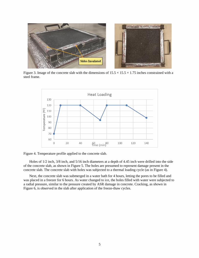
constrained with a steel frame shown in Figure 3. Heat was applied to the bottom of the concrete slab
using a silicone thermal blanket as per the temperature profile, shown in Figure 4, to induce strains in the
slab due to thermal expansion. To reduce heat loss in the concrete sample due to the convection and
conduction effects between the thermal blanket and the steel frame, insulation sheets were installed. The
heat blanket was covered with a rectangular insulation sheet. Moreover, the frame’s sides were wrapped
with the insulation material. The material properties of the sheet determined the maximum temperature
applied to the sample, its melting temperature is 160°F, but for precaution a lower temperature was used.
The initial temperature of the slab and equipment was 70°F, which is the ambient temperature in the
Laboratory for Systems Integrity and Reliability (LASIR). Each thermal cycle had a total duration of 70
minutes. During the first 10 minutes of the first thermal cycle, the blanket temperature increased to 120°F.
The temperature was held at 120°F for 30 minutes and then for the next 30 minutes the HEATCON® unit
was turned off to allow the temperature to drop to 95°F. The second cycle was similar to the first cycle,
but the positive slope differed from the first cycle. The positive slope for the first cycle was 5°F/min and
for the second cycle was 3°F/min.
Figure 2. Image of the concrete slab with the dimensions of 15.5 × 15.5 × 1.75 inches.
5
Figure 3. Image of the concrete slab with the dimensions of 15.5 × 15.5 × 1.75 inches constrained with a
steel frame.
Figure 4. Temperature profile applied to the concrete slab.
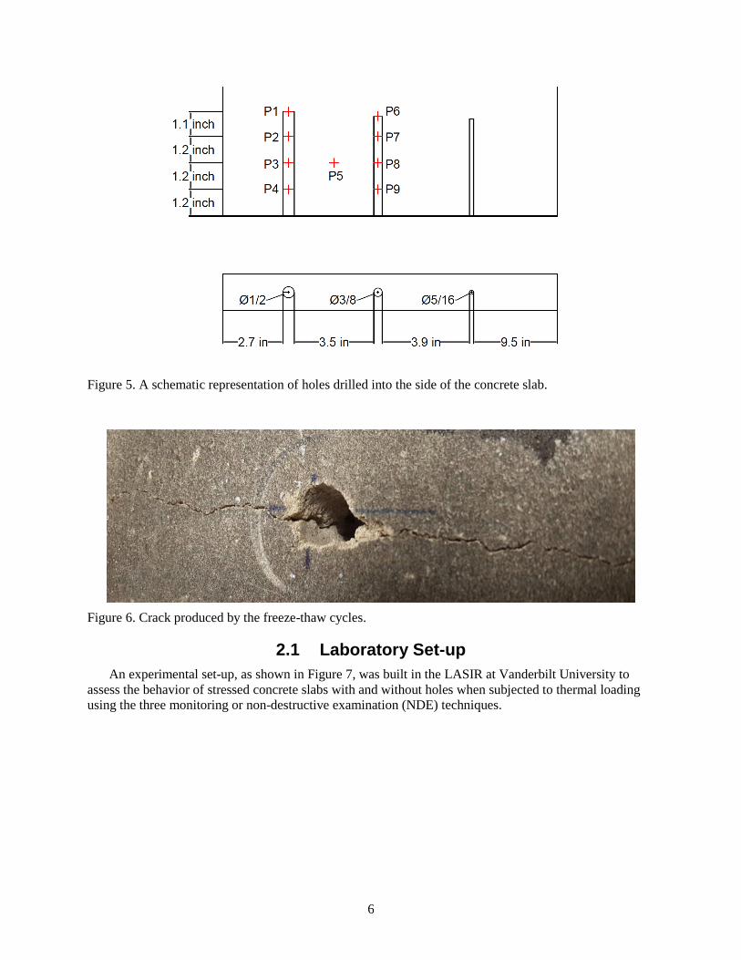
Holes of 1/2 inch, 3/8 inch, and 5/16 inch diameters at a depth of 4.45 inch were drilled into the side
of the concrete slab, as shown in Figure 5. The holes are presumed to represent damage present in the
concrete slab. The concrete slab with holes was subjected to a thermal loading cycle (as in Figure 4).
Next, the concrete slab was submerged in a water bath for 4 hours, letting the pores to be filled and
was placed in a freezer for 6 hours. As water changed to ice, the holes filled with water were subjected to
a radial pressure, similar to the pressure created by ASR damage in concrete. Cracking, as shown in
Figure 6, is observed in the slab after application of the freeze-thaw cycles.
6
Figure 5. A schematic representation of holes drilled into the side of the concrete slab.
Figure 6. Crack produced by the freeze-thaw cycles.
2.1 Laboratory Set-up
An experimental set-up, as shown in Figure 7, was built in the LASIR at Vanderbilt University to
assess the behavior of stressed concrete slabs with and without holes when subjected to thermal loading
using the three monitoring or non-destructive examination (NDE) techniques.

7
Figure 7. An experimental set-up in the LASIR at Vanderbilt University. (Left) Concrete slab with holes
along with the ultrasonic measurement unit. (Right) Concrete slab with thermography imaging and DIC
measuring units.
For thermography imaging, FLIR® Infrared (IR) camera was used to detect the temperature contours
on the surface of the concrete slab. These contours were analyzed to detect flaws or defects in the slabs
that cannot be easily detected by visual inspection. For DIC, two high-speed video cameras to track the
motion of speckles painted onto the surface of the slab were utilized. The speckles are produced due to
strain and deformation of the concrete slab during the duration of the cyclic thermal loading. Both FLIR®
IR camera and DIC were set up to capture images of the concrete slab every 2 minutes. For ultrasonic
inspection, a General Electric Phased array unit was used to detect the damage in the slab by sending out
a signal and measuring the time of flight of the transmitted signal when it reflects from each surface in the
material (for example, cracks, holes, or large aggregate). The density of the material is used along with a
5 MHz ultrasonic probe to detect the location and depth of holes and cracks in the concrete samples.
In addition, the HEATCON® composite system controller was connected to the thermal blanket and
used to program a defined thermal cycle that can be repeated as many times as needed for a test. Two
thermocouples were used to measure and monitor the heat applied by thermal blanket. One thermocouple
was placed beneath the blanket and the other thermocouple was place between the thermal blanket and the
concrete sample, as shown in Figure 8.
Figure 8. Location of the two thermocouples used to measure and monitor the heat applied by the thermal
blanket.

8
For this demonstration example, the four stages of concrete structure status considered include, slab
with no holes, slab with holes, slab subjected to freeze-thaw Cycle 1, and slab subjected to freeze-thaw
Cycle 2. In each stage, both FEA modeling and NDE monitoring techniques are employed. After
analyzing the NDE data, temperature and strain distribution, and crack configuration are obtained. The
temperature and strain distribution obtained during the first two stages is used to calibrate unknown
parameters of a FEA model. Using the Bayesian calibration, the posterior distribution of unknown
parameters is obtained. The outcomes from experiments and models are integrated into dynamic Bayesian
network to do Bayesian calibration, diagnosis, and prognosis. Specifically, the diagnosis of crack
configuration is performed after the first freeze-thaw cycle in Stage 3, and the prognosis of future crack
configuration is performed after the second freeze-thaw cycle in Stage 4. The uncertainty associated with
the crack configuration diagnosis is utilized to predict future crack configuration in Stage 4. The flow
chart in Figure 9 summarizes how the four elements of the proposed framework are integrated during four
stages.
Figure 9. Flow chart showing the connections of the measured data to the four elements of the proposed
SHM framework.

9
3. DAMAGE MODELING
The demonstration example only considered mechanical damage and no chemical mechanisms. Thus,
the modeling was performed at the macro-level; using the commercially available Abaqus FEA software
(2011) to develop finite element models of concrete slabs. The model configurations shown in Figure 10,
were used for FEA during the first two stages:
1. Concrete slab without holes
2. Concrete slab with three holes drilled into the side edge, with 1/2 inch, 3/8 inch and 5/16 inch
diameters and a depth of 4.45 inch.
Figure 10 Model configuration in Abaqus for slabs (Left) without holes and (Right) with holes.
Three (3) FEA models were created for the slab, representing the three stages considered: (1) slab
without holes, (2) slab with the holes, and (3) slab with the holes subjected to freeze-thaw cycle. Each of
the three models is subjected to two types of boundary conditions, corresponding to the experimental
setup: (1) free edges and (2) constrained edges. Solid homogeneous sections were used for finite element
modeling. In the material property module, the properties shown in Table 1 were assigned to the model.
The properties were selected based on the research performed by Xu and Chung (2000).
Table 1. Material properties.
Density 1.99 gm/cm3
Young’s Modulus 2.92 GPa
Coefficient of thermal expansion 1×10⁻⁵
Specific heat 0.703 J/g K
Thermal conductivity ( ) 0.33−0.72 W/(mK)
Coefficient of convection ( ) 5−25 W/m2K
The slab was subjected to two cycles of heat loading as described in Section 2. The initial temperature
of the slab was set at the room temperature of 70°F. The temperature cycles were applied at one surface,
as shown in Figure 11, consistent with the thermal loading applied by using the thermal blanket for the
laboratory experiments.
Drilled holes
10
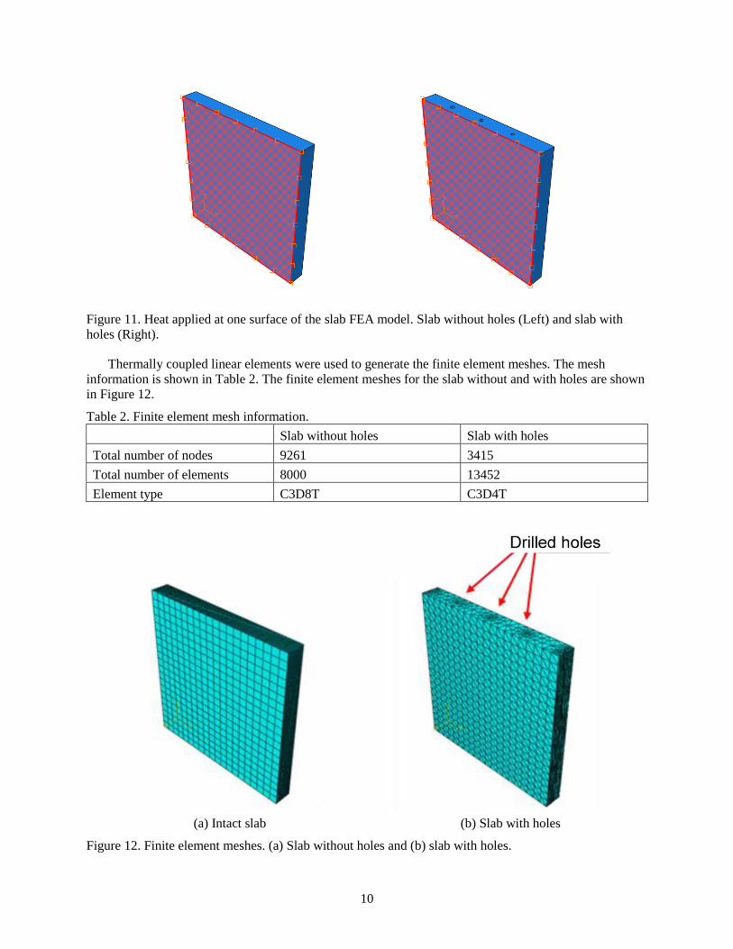
Figure 11. Heat applied at one surface of the slab FEA model. Slab without holes (Left) and slab with
holes (Right).
Thermally coupled linear elements were used to generate the finite element meshes. The mesh
information is shown in Table 2. The finite element meshes for the slab without and with holes are shown
in Figure 12.
Table 2. Finite element mesh information.
Slab without holes Slab with holes
Total number of nodes 9261 3415
Total number of elements 8000 13452
Element type C3D8T C3D4T
(a) Intact slab (b) Slab with holes
Figure 12. Finite element meshes. (a) Slab without holes and (b) slab with holes.

11
The structural models were used to compute temperature and maximum principal strain at the
midpoint of the surface opposite to the thermal loading surface. Temperature response results for the slab
without holes and slab with holes are shown in Figure 13. The contours show areas where holes are
present for the slab with holes. The maximum principal strain response results for the slab without holes
and slab with holes are shown in Figure 14. The contours show areas where holes are present (Figure
14(b)).
(a) Slab without holes (b) Slab with holes
Figure 13. Temperature contours. (a) Slab without holes and (b) slab with holes.
(a) Slab without holes (b) Slab with holes
Figure 14. Strain contours. (a) Slab without holes and (b) slab with holes.
The material parameters considered in Table 1 are random quantities. Of these parameters, thermal
conductivity ( ) and coefficient of convection ( ) have major impact on the temperature and strain
results. These two parameters were considered sources of epistemic uncertainties in this demonstration.
The parameters and are considered to have a range of values as shown in Table 1. Twenty-five
(25) pairs of and values were generated by the Latin hypercube design of experiment explained in
Section 6.1.
The temperature and maximum principal strain outputs were obtained from the structural FEA model for
the different pairs of and .
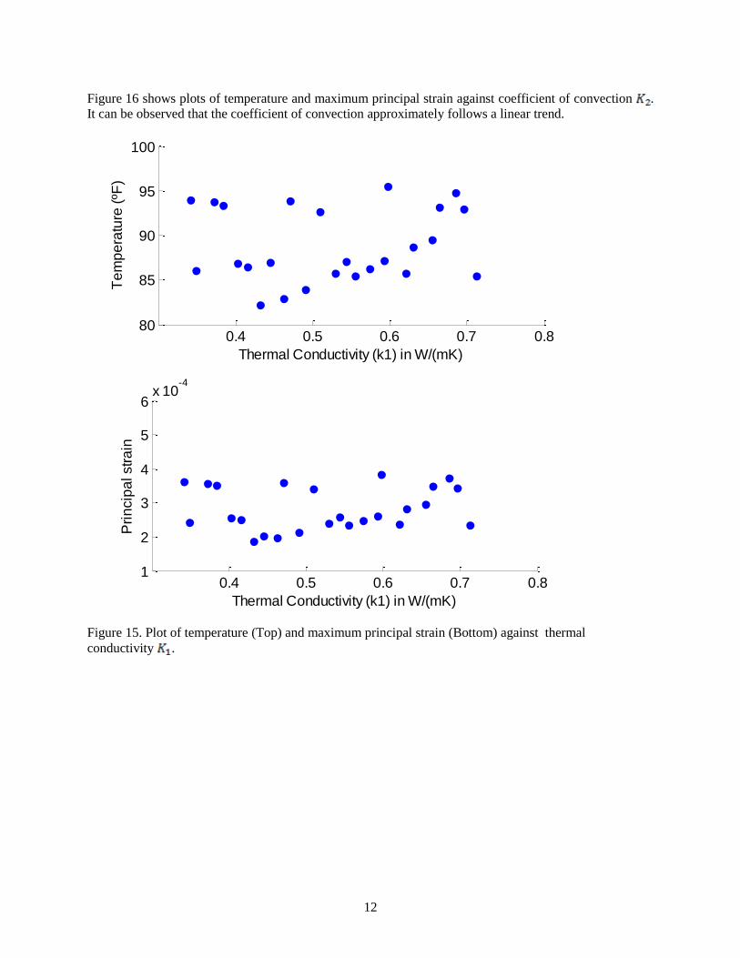
Figure 15 shows scattered plots of temperature and maximum principal strain against thermal
conductivity. It can be observed that there is no trend for thermal conductivity. On the other hand,
12
Figure 16 shows plots of temperature and maximum principal strain against coefficient of convection .
It can be observed that the coefficient of convection approximately follows a linear trend.
0.4 0.5 0.6 0.7 0.880
85
90
95
100
Thermal Conductivity (k1) in W/(mK)
Te
mp
era
ture
(ºF
)
0.4 0.5 0.6 0.7 0.81
2
3
4
5
6x 10
-4
Thermal Conductivity (k1) in W/(mK)
Pri
ncip
al str
ain
Figure 15. Plot of temperature (Top) and maximum principal strain (Bottom) against thermal
conductivity .

13
5 10 15 20 2580
85
90
95
100
Coefficient of convection (k2) in W/m2K
Te
mp
era
ture
(ºF
)
5 10 15 20 251
2
3
4
5
6x 10
-4
Coefficient of convection (k2) in W/m2K
Pri
ncip
al str
ain
Figure 16. Plot of temperature (Top) and maximum principal strain (Bottom) against coefficient of
thermal convection .
These results were used to build a surrogate model for Bayesian calibration of and . The
surrogate mode is explained in Section 6.
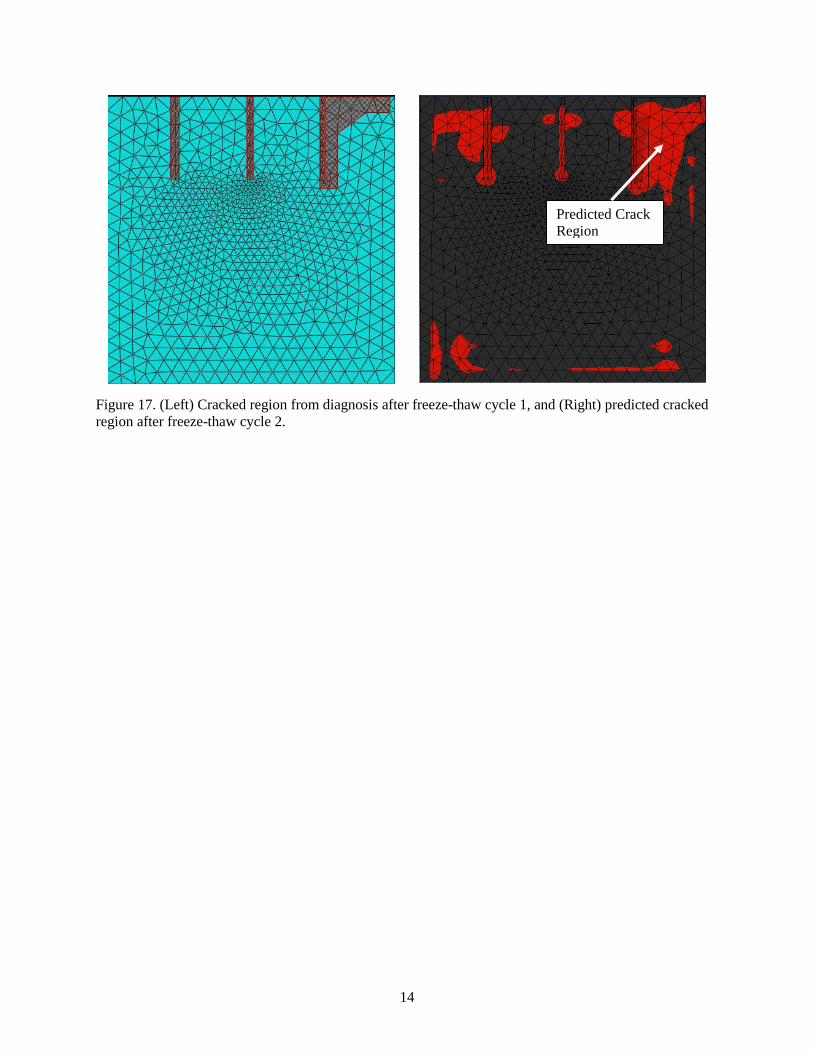
In the next stage, the cracks generated due to freeze-thaw cycles were incorporated in the finite
element model. The crack diagnosis is done by data analytics described in Section 3.1.6. The finite
element model is used for prognosis. Figure 17 shows the predicted crack locations at the center of the
slab after another freeze-thaw cycle using the calibrated values of and .
Six sets of crack diagnoses using different features were obtained from data analytics and
corresponding crack areas were predicted using the model. This prediction result is used in Section 6.1.2
for uncertainty quantification of crack growth.
14
Figure 17. (Left) Cracked region from diagnosis after freeze-thaw cycle 1, and (Right) predicted cracked
region after freeze-thaw cycle 2.
Predicted Crack
Region

15
4. MONITORING
Based on the initial review of literature, presentations, and discussions on current activities related to
concrete structures deterioration modeling and monitoring at the workshop (Mahadevan et al., 2014), this
research will investigate monitoring of physical and mechanical coupled degradation in concrete via
full-field imaging techniques. Effective combinations of full-field techniques should be identified for
different types of concrete structures under different loading and operating conditions. In this report,
possible full-field techniques include infrared imaging, DIC, and ultrasonic. This section briefly discusses
these techniques.
Infrared thermography maps the thermal load path in a material. In the case of concrete, cracking,
spalling, and delamination all create a discontinuity in the thermal load path. Additionally, rebar and
tensioning cables can be easily detected due to the difference in thermal conductivity coefficients between
steel and concrete. Thermography has even been shown to detect debonding between the reinforcing steel
and concrete. Infrared thermography can be either an active or passive monitoring technique. When heat
is locally added to the structure to create a temperature gradient, it is referred to as active. If the solar heat
is used to provide heat to produce the temperature gradient, it is considered passive. Passive infrared
thermography is preferred because it is less energy intensive. Electric Power Research Institute (EPRI)
showed the feasibility of infrared thermography by mapping a 450,000ft2 dam. During the 2 days that
EPRI spent mapping the dam, numerous potential delamination sites were identified (Renshaw, 2014).
Kobayashi and Banthia (2011) combined induction heating with infrared thermography to detect
corrosion in reinforced concrete. Induction heating uses electromagnetic induction to produce an increase
in temperature in the rebar. When corrosion is present, it inhibits the diffusion of heat from the rebar to
the surrounding concrete. Infrared thermography is then used to capture the temperature gradient. It was
concluded that the temperature rise in corroded rebar is higher than that in a non-corroded rebar, a more-
corroded rebar yields a smaller temperature rise on the surface, and the technique is more effective with
larger bar diameters and smaller cover depths (Kobayashi and Banthia, 2011). Further research may be in
order to evaluate the combination of induction heating and infrared thermography as a means to identify
debonded rebar.
Digital Image Correlation is an optical NDE technique. It can be conducted quickly, which allows it
to be used as a screening method. DIC is capable of measuring deformation, displacement, and strain of a
structure (Bruc, 2012). During a NPP routine pressure tests on the containment vessels, when the internal
pressure reaches 60 psi, it would provide an ideal condition to use DIC to determine the deformation of
the concrete containment. DIC is capable of detecting surface defects such as cracks, micro-cracks, and
spalling, but is unable to detect any subsurface defects. DIC is commercially available.
Ultrasonic testing utilizes high-frequency oscillating sound pressure waves. In a recent study led by
ORNL, five NDE techniques were evaluated, including shear-wave ultrasound and semi-coupled
ultrasonic tomography. The shear-wave ultrasound consisted of a 4 × 12 array that was capable of
producing real time three-dimensional imaging. The semi-coupled ultrasonic tomography was excellent at
identifying internal void areas and unbonded, embedded rebar. Both techniques did show some
limitations; the semi-coupled ultrasonic tomography was unable to detect well-bonded rebar, and the
shear-wave ultrasound is in need of post-processing of the data. The shear-wave ultrasound is currently in
commercial production, but the semi-coupled ultrasonic tomography is not (Clayton, 2014).
The slabs were heated with the thermal blanket and the data was collected using DIC, infrared
thermography, and ultrasonic measurement. The concrete slab was tested under three conditions:
(1) without holes, (2) with holes, and (3) with holes and freeze-thaw cycling. The concrete slab was tested
with and without the steel frame to better understand the effect of boundary conditions on the results.
16
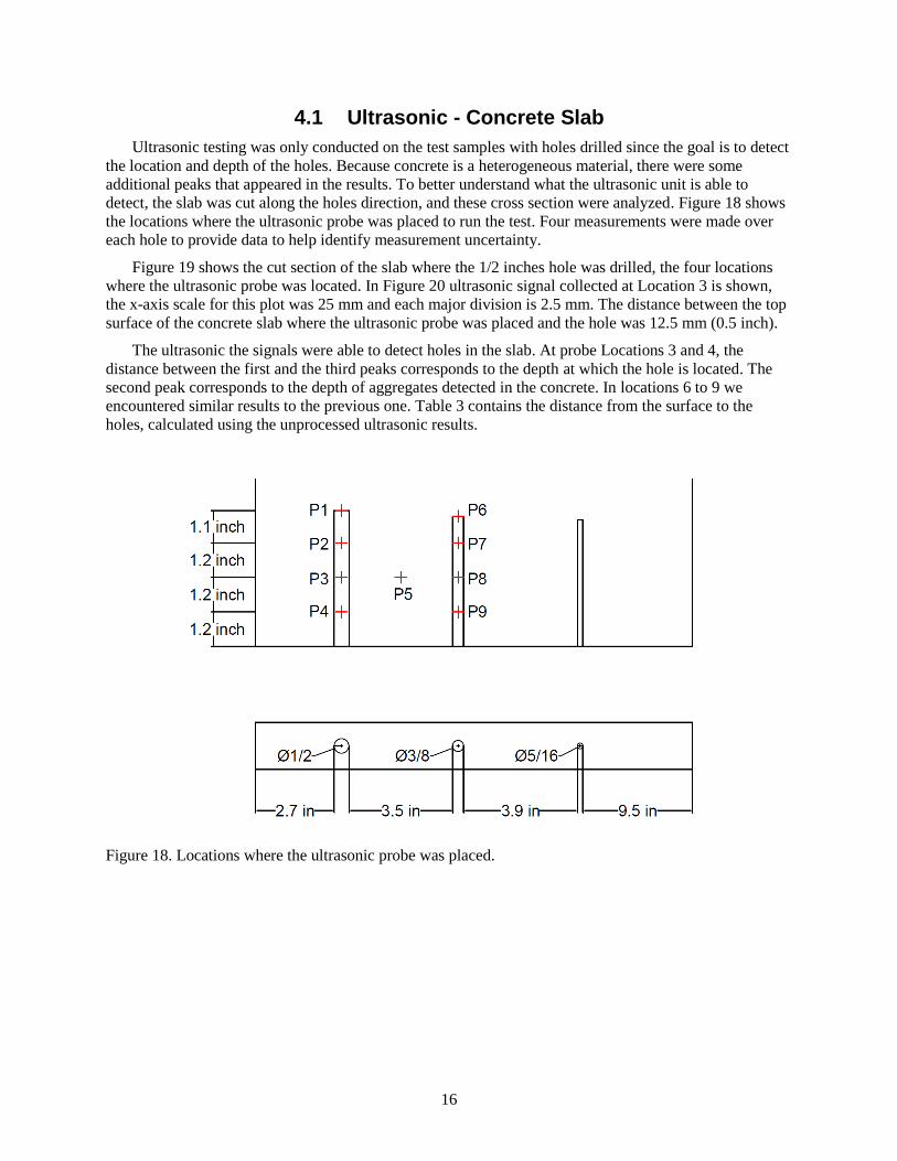
4.1 Ultrasonic - Concrete Slab
Ultrasonic testing was only conducted on the test samples with holes drilled since the goal is to detect
the location and depth of the holes. Because concrete is a heterogeneous material, there were some
additional peaks that appeared in the results. To better understand what the ultrasonic unit is able to
detect, the slab was cut along the holes direction, and these cross section were analyzed. Figure 18 shows
the locations where the ultrasonic probe was placed to run the test. Four measurements were made over
each hole to provide data to help identify measurement uncertainty.
Figure 19 shows the cut section of the slab where the 1/2 inches hole was drilled, the four locations
where the ultrasonic probe was located. In Figure 20 ultrasonic signal collected at Location 3 is shown,
the x-axis scale for this plot was 25 mm and each major division is 2.5 mm. The distance between the top
surface of the concrete slab where the ultrasonic probe was placed and the hole was 12.5 mm (0.5 inch).
The ultrasonic the signals were able to detect holes in the slab. At probe Locations 3 and 4, the
distance between the first and the third peaks corresponds to the depth at which the hole is located. The
second peak corresponds to the depth of aggregates detected in the concrete. In locations 6 to 9 we
encountered similar results to the previous one. Table 3 contains the distance from the surface to the
holes, calculated using the unprocessed ultrasonic results.
Figure 18. Locations where the ultrasonic probe was placed.

17
Figure 19. Cross section of the 0.5-inch-diameter hole.
Figure 20. Ultrasonic signal at Location 3 (the two peaks are marked with circles).
18
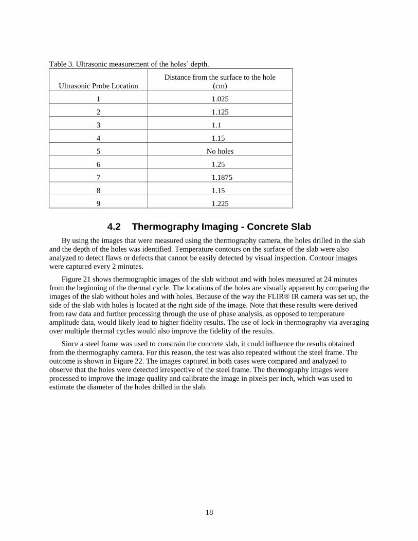
Table 3. Ultrasonic measurement of the holes’ depth.
Ultrasonic Probe Location
Distance from the surface to the hole
(cm)
1 1.025
2 1.125
3 1.1
4 1.15
5 No holes
6 1.25
7 1.1875
8 1.15
9 1.225
4.2 Thermography Imaging - Concrete Slab
By using the images that were measured using the thermography camera, the holes drilled in the slab
and the depth of the holes was identified. Temperature contours on the surface of the slab were also
analyzed to detect flaws or defects that cannot be easily detected by visual inspection. Contour images
were captured every 2 minutes.
Figure 21 shows thermographic images of the slab without and with holes measured at 24 minutes
from the beginning of the thermal cycle. The locations of the holes are visually apparent by comparing the
images of the slab without holes and with holes. Because of the way the FLIR® IR camera was set up, the
side of the slab with holes is located at the right side of the image. Note that these results were derived
from raw data and further processing through the use of phase analysis, as opposed to temperature
amplitude data, would likely lead to higher fidelity results. The use of lock-in thermography via averaging
over multiple thermal cycles would also improve the fidelity of the results.
Since a steel frame was used to constrain the concrete slab, it could influence the results obtained
from the thermography camera. For this reason, the test was also repeated without the steel frame. The
outcome is shown in Figure 22. The images captured in both cases were compared and analyzed to
observe that the holes were detected irrespective of the steel frame. The thermography images were
processed to improve the image quality and calibrate the image in pixels per inch, which was used to
estimate the diameter of the holes drilled in the slab.
19

20
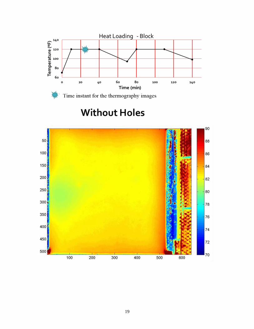
Figure 21. Thermographic images of the slab without holes (Upper) and with holes (Lower) at 24
minutes. The holes are indicated with arrows.

21
Slab with frame
34.6 oF
87.4 oF

22
87.4 oF
34.6 oF

23
Slab without frame
70.7 oF
106.8 oF

24
Figure 22. Thermographic images of concrete slab with and without the steel frame at 18 minutes:
Without holes (Upper) and with holes (Lower)
4.3 Digital Image Correlation
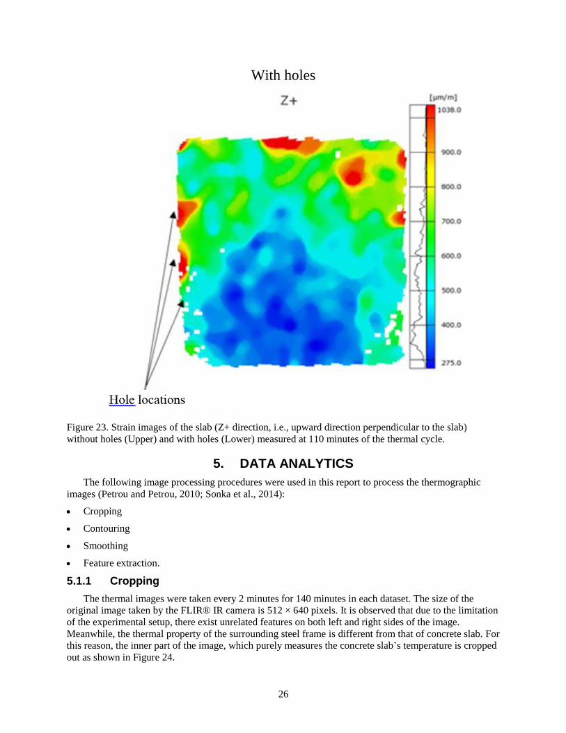
DIC was used to obtain strain data. Figure 23 shows strain images of the slab without holes and the
slab with the holes, measured at 110 minutes of the thermal cycle. Because of the way in which the
equipment was set up, the holes are located on the left side of the slab in the strain images, as indicated in
Figure 23. The larger holes are located in the upper half of the slab. The results verify that the strain
values at the location where the large holes were located are significantly higher than in the rest of the
slab. Also, the strain is largest at the edge of the slab where the two largest holes are located compared to
the strain in the slab without holes.
70.7 oF
106.8 oF

25
Without holes
26
With holes
Figure 23. Strain images of the slab (Z+ direction, i.e., upward direction perpendicular to the slab)
without holes (Upper) and with holes (Lower) measured at 110 minutes of the thermal cycle.
5. DATA ANALYTICS
The following image processing procedures were used in this report to process the thermographic
images (Petrou and Petrou, 2010; Sonka et al., 2014):
Cropping
Contouring
Smoothing
Feature extraction.
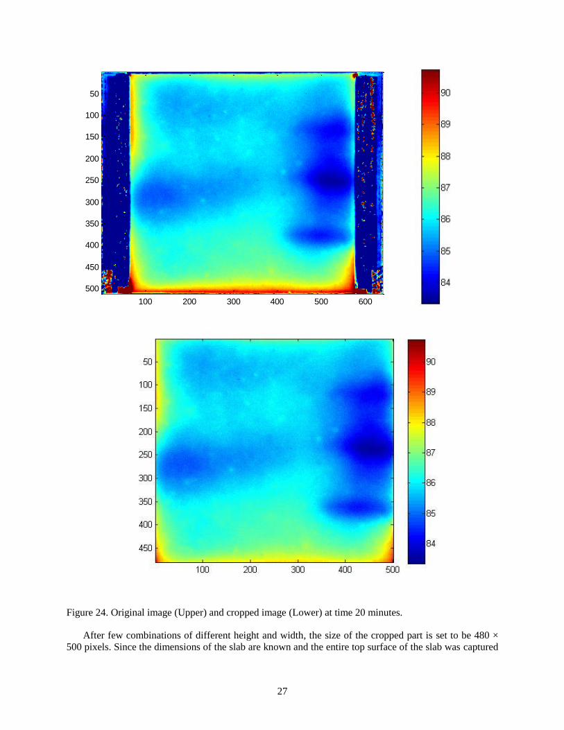
5.1.1 Cropping
The thermal images were taken every 2 minutes for 140 minutes in each dataset. The size of the
original image taken by the FLIR® IR camera is 512 × 640 pixels. It is observed that due to the limitation
of the experimental setup, there exist unrelated features on both left and right sides of the image.
Meanwhile, the thermal property of the surrounding steel frame is different from that of concrete slab. For
this reason, the inner part of the image, which purely measures the concrete slab’s temperature is cropped
out as shown in Figure 24.
27
100 200 300 400 500 600
50
100
150
200
250
300
350
400
450
500
Figure 24. Original image (Upper) and cropped image (Lower) at time 20 minutes.
After few combinations of different height and width, the size of the cropped part is set to be 480 ×
500 pixels. Since the dimensions of the slab are known and the entire top surface of the slab was captured

28
within the thermographic images, a relationship of the dimension of the slab to the pixel-wise information
was calculated:
1 pixel = 0.0777 cm or 12.86 pixel/cm
This pixel-to-length conversion is helpful in localization and quantification of the defects or damage.
This cropping process is carried out first for each of the thermographic images provided by the
experiments, before the subsequent image processing steps were applied. For the experiment of the same
slab, as long as the fixtures remained unmoved, the cropping method stays the same. A new decision
about the cropping criterion should be considered for each different experimental setup, especially if the
position of the fixture and test sample has been changed.
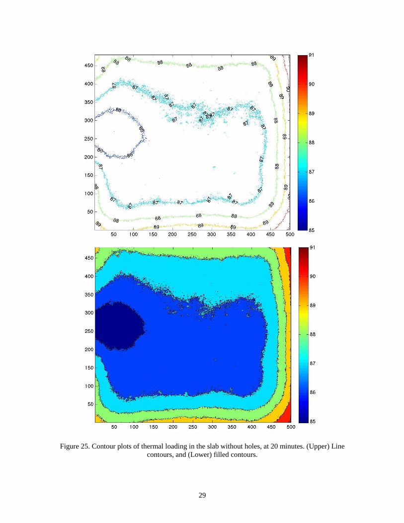
5.1.2 Contouring
Contour lines depict the crossing point of a genuine or speculative surface with one or more level
planes. The configuration of these contours permits us to deduce relative inclination of a parameter and
appraisal of that parameter at particular spots. In this research, contours could assist in approximately
identifying the damaged zone. It is extremely useful for feature extraction.
Figure 25and Figure 26 show temperature contours in the slab after 20 minutes of thermal loading,
without holes and with holes. The holes are visually observable in the second image in Figure 246.
29
Figure 25. Contour plots of thermal loading in the slab without holes, at 20 minutes. (Upper) Line
contours, and (Lower) filled contours.

30
Figure 26. Contour plots of temperature in the slab with holes, at 20 minutes. (Upper) Line contours, and
(Lower) filled contours.

31
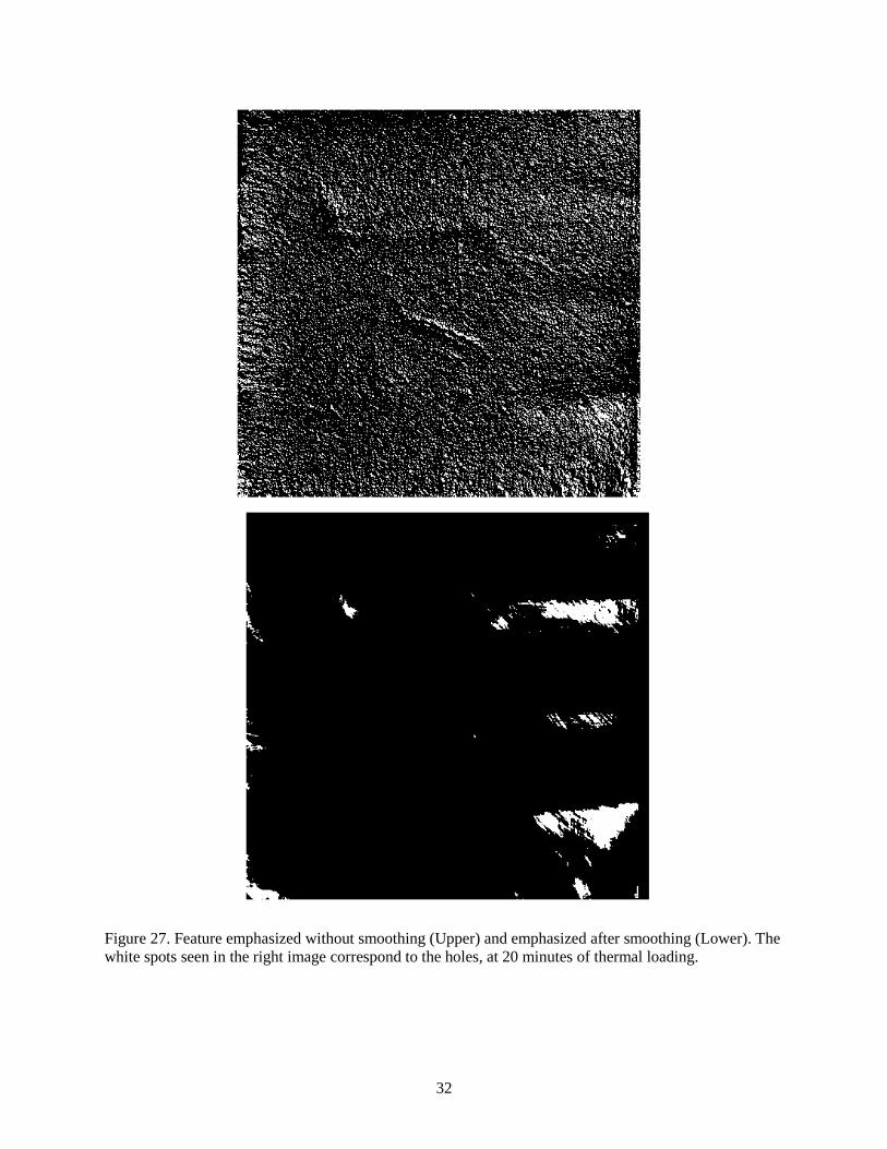
5.1.3 Smoothing
Due to operational and experimental imperfection, the image captured has a significant level of noise,
as shown in Figure 27. Therefore, smoothing is an important step in image processing. Smoothing of
information set is done to make an approximation that endeavors to catch the essential information, while
ignoring noise (or other fine-scale structures) and transient phenomena. In smoothing, the details of a
feature can be altered, so individual pixels (possibly as a result of commotion) are diminished, and pixels
that are lower in magnitude than the neighboring pixels are expanded, prompting a smoother feature.
Smoothing could be utilized into the two following significant aspects for data analytics.
There are a couple of methods for smoothing the data. The simple moving average (SMA) method is
classical and effective. More complicated smoothing methods also exist, such as Butterworth filter,
Kalman filter, etc. The smoothing method applied in this study to the thermographic images is a
two-dimensional SMA, which uses the following equation:
(1)
where represents each of the values within a moving window. In our two-dimensional cases, the size-n
moving window is replaced by an n by n matrix. The SMA method is quite simple, yet the effect is
significant. After a few tests, a window size of n = 25 is seen to be satisfactory. Figure 27 shows
comparisons of the features before and after the application of SMA.
Note that Figures 27 to 30 are in gray scale, since the detection of holes/cracking is a binary classification
problem. The image features guide us to make the decision, whether a region of the slab is damaged or
not, represented by 1 or 0. Therefore black and white is easier to show the diagnosis decision making
instead of color scale.
32
Figure 27. Feature emphasized without smoothing (Upper) and emphasized after smoothing (Lower). The
white spots seen in the right image correspond to the holes, at 20 minutes of thermal loading.

33
5.1.4 Feature Extraction
From the contour images shown in Figure 26, differences are seen between the contours of the slab
without and with holes. However, a simple baseline removal method or simple gradient method is not
effective enough to provide feature classification capability. Texture detection provided an additional
opportunity to improve the classification of features in the image. Instead of simply classifying features
by the temperature contour value or temperature value, the distribution of the colors is used because it is
easier for visual classification of damage. The gradient-based approach has been found to be significantly
effective in face recognition, human recognition, and object detection studies. The feature developed here
is gradient-based with baseline data subtracted from the observed data.
The gradient of an image is given by the formula,
, (2)
where is the gradient in the x direction, is the gradient in the y direction.
The gradient direction can be calculated by the formula:
(3)
To calculate the feature, the gradient along the x and y directions of the images was calculated for the
observed cases with baseline data subtracted. To describe the specific contour texture in the image, a
characteristic value (or threshold value) was defined. In this study, after a few trials, based on the
distributions of gradients along x-axis and y-axis, a threshold value of 0.1 was set. The specific texture
was defined when is less than the threshold value and is greater than the threshold value. The
images in Figure 28 are the classification results based on the features extracted by applying the gradient
method to the images for the slab with holes using the frame and with the frame removed. For the images
shown in Figure 28, the white spots indicate the holes. The presence or absence of the frame changes the
boundary condition and the heat transfer within the slab, thus explaining the difference in the two images.
Further experiments are done with the frame.
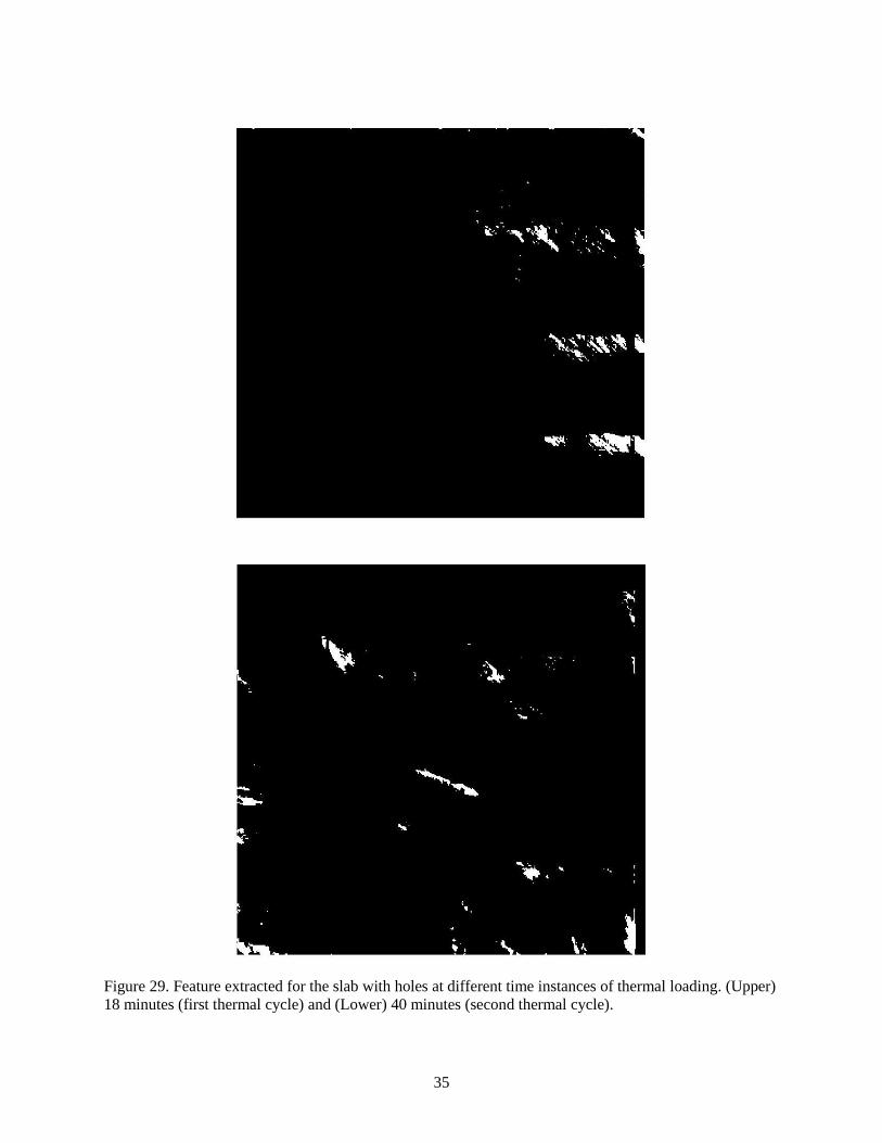
The creation of this feature took several iterations that highlighted another issue. The selection of the
time instant of the data affects the performance of this damage diagnosis feature. The images in Figure 29
show the features that were extracted from the image of slab with holes (with the frame removed) at
different time instances. It is seen from Figure 29 that only the data collected during the first heating stage
is valuable, and not the data from the latter stage. This is expected in thermography, where the best
contrast is usually seen during the application of increasing temperature.
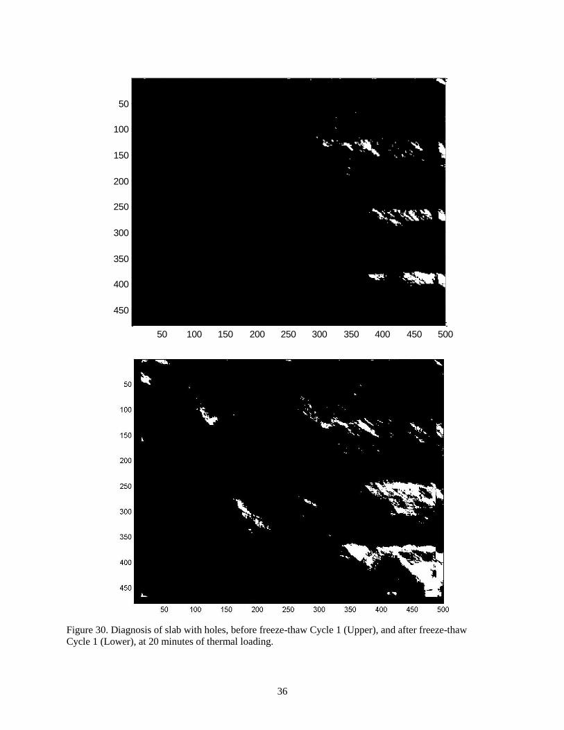
5.1.5 Crack Diagnosis after Freeze-Thaw Cycle 1
As mentioned in Section 2, the concrete slab with holes is subject to freeze-thaw cycles to induce
cracking. Thermography images collected after freeze-thaw Cycle 1 are used for the diagnosis. The
images from the slab without and with holes were used as baselines and image processing procedures
described above were used to accomplish the diagnosis shown in Figure 30.
Data analytics of the thermography image collected after freeze-thaw Cycle 1 indicates cracking near
two of the holes, as shown in Figure 30. The same analysis, when repeated with six different settings for
the selected features, gave slightly different cracking configurations; only one of them is shown as
illustration in Figure 30. Combining these six different analyses, the probabilistic diagnosis result is
reported as: mean cracked area = 9.44 inch, and standard deviation of cracked area = 2.11 inch.

34
Figure 28. Feature extracted for the slab with holes. (Upper) With steel frame and (Lower) with steel
frame removed, at 20 minutes of thermal loading.
35
Figure 29. Feature extracted for the slab with holes at different time instances of thermal loading. (Upper)
18 minutes (first thermal cycle) and (Lower) 40 minutes (second thermal cycle).
36
50 100 150 200 250 300 350 400 450 500
50
100
150
200
250
300
350
400
450
Figure 30. Diagnosis of slab with holes, before freeze-thaw Cycle 1 (Upper), and after freeze-thaw
Cycle 1 (Lower), at 20 minutes of thermal loading.

37
6. UNCERTAINTY QUANTIFICATION
6.1 Background
6.1.1 Dynamic Bayesian Network
Bayesian Networks are directed acyclic graphical representations with nodes to represent the random
variables and arcs to show the conditional dependencies among the nodes (Jensen, 1996). Pointed from
parent node to child node, each arc carries a conditional probability function. The entire network can be
represented using a joint probability density function. A Dynamic Bayesian Network (DBN) is a Bayesian
Network that relates variables to each other over adjacent time steps. Both forward and inverse problems
can be performed using DBN. Forward problems include uncertainty propagation to calculate system
output prediction uncertainty, which in the context of this report implies prognosis. Two types of inverse
problems are supported by the DBN: (1) uncertainty quantification in the diagnosis of damage state, and
(2) calibration of unknown parameters. In both cases, a prior distribution is assumed for the damage state
or the unknown parameter, and a posterior distribution is computed using the observed data. Markov
chain Monte Carlo (MCMC) simulation is commonly used for the inverse problem, which requires a large
number of samples. If the original system model is expensive (e.g., finite element model, as in this
demonstration problem), MCMC is unaffordable. Therefore, a surrogate model is used to replace the
Finite Element model, as described in the next subsection.
Figure 31sent observed data. A solid line arrow represents a conditional probability link, and a dashed
line arrow represents the link of a variable to its observed data if available. In Figure 31, a system level
output is a function of two subsystem level quantities and ; in turn, is a function of
subsystem-level input and model parameter , and similarly, is a function of subsystem-level
input and model parameter . Experimental data with the respective model predictions .
Figure 31. Bayesian Network illustration.
For the problem in Figure 31 uncertainty propagation can be expressed as:
(4)
(5)
(6)
And parameter calibration can be accomplished as:
(7)

38
6.1.2 Gaussian Process Surrogate Model
The benefit of using a surrogate model is to greatly shorten the computational effort for Bayesian
updating and uncertainty quantification, by replacing the time-consuming system model (e.g., finite
element model). Many different types of surrogate models are available, such as polynomial response
surfaces, Kriging, support vector machines, space mapping, and artificial neural networks. The Gaussian
process (GP) surrogate model is one kind of Kriging model, which is a stochastic process whose
realizations consist of random variables associated with every point along the coordinate such that each
such random variable has a normal distribution (Rasmussen and Williams, 2006). Formally, a Gaussian
process generates data located throughout some domain such that any finite subset of the range follows a
multivariate Gaussian distribution. The mean of GP could be zero, a constant, or any appropriate trend
function. If a stationary GP is assumed, then one observation is related to another through the covariance
function, . A popular choice is the “squared exponential,”
(8)
where is the process variance.
To prepare the GP model, covariance functions should be calculated first:
(9)
In GP modeling, data can be represented as a sample from a multivariate Gaussian distribution, as:
(10)
where T indicates matrix transpose. The prediction at a desired value of x follows a Gaussian distribution:
(11)
A one-dimensional example is shown in Figure 32. In this example, the original model is
, which has single input and output. It can be observed that the GP surrogate model
predicts the exact value at the training points, while the variance increases at locations away from the
training points. A multiple-input GP surrogate model can also be created, and the prediction will behave
the same way.

39
Figure 32. Gaussian process surrogate model example.
To train a GP model of high quality, training datasets should be selected to be representative of the
prediction scenario, and ensure full coverage of the scenarios of interest. Thus design of experiment is an
important step.
Design of experiment is a systematic method to determine the relationship between inputs affecting a
process and the output of that process. The Latin Hypercube random sampling method was used in this
example. When sampling a function of N variables, the range of each variable is divided into M in equally
probable intervals. M sample points are then generated to ensure uniform coverage of the space spanned
by the ranges of the variables.
6.2 Uncertainty Quantification of the Demonstration Problem: Calibration, Diagnosis and Prognosis
A DBN is employed for uncertainty quantification in calibration, diagnosis, and prognosis. Three
states of the concrete slab are considered: slab without holes, slab with holes, slab with holes subjected to
freeze-thaw cycles. Each state happens at a discrete time step. Within the first two time steps,
temperature-loading history ( , which is applied as boundary condition) is the input, and temperature
at the top surface of slab ( ) and maximum principal strain at the top center ( ) is the output. Seven
material parameters are required for the model prediction: (Young’s Modulus), (Poisson’s ratio),
(coefficient of thermal expansion), (specific heat), (density), (thermal conductivity),
(convection). For the sake of illustration, we assume and need to be calibrated, while the other
variables are known constants.
40
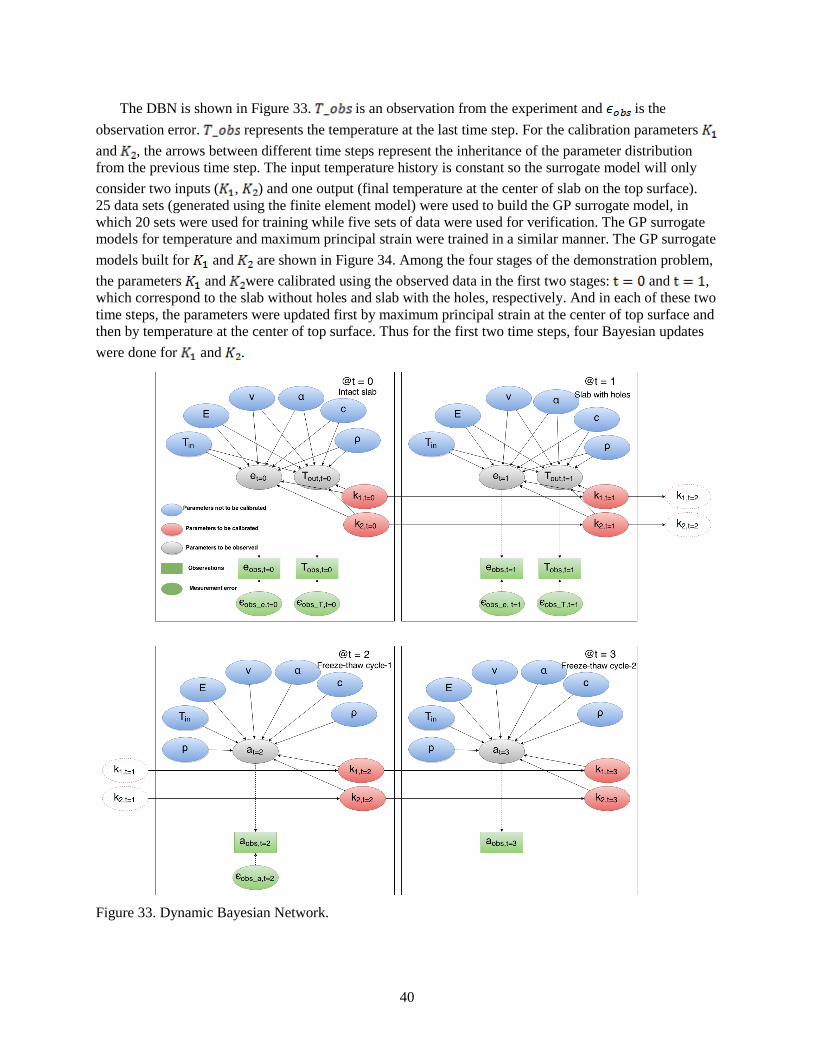
The DBN is shown in Figure 33. is an observation from the experiment and is the
observation error. represents the temperature at the last time step. For the calibration parameters
and , the arrows between different time steps represent the inheritance of the parameter distribution
from the previous time step. The input temperature history is constant so the surrogate model will only
consider two inputs ( , ) and one output (final temperature at the center of slab on the top surface).
25 data sets (generated using the finite element model) were used to build the GP surrogate model, in
which 20 sets were used for training while five sets of data were used for verification. The GP surrogate
models for temperature and maximum principal strain were trained in a similar manner. The GP surrogate
models built for and are shown in Figure 34. Among the four stages of the demonstration problem,
the parameters and were calibrated using the observed data in the first two stages: and ,
which correspond to the slab without holes and slab with the holes, respectively. And in each of these two
time steps, the parameters were updated first by maximum principal strain at the center of top surface and
then by temperature at the center of top surface. Thus for the first two time steps, four Bayesian updates
were done for and .
Figure 33. Dynamic Bayesian Network.

41
(a) (b)
Figure 34. GP surrogate model for healthy slab (a) and damaged slab (b), ( ) vs .
The posterior distribution of and is treated as the prior distribution for the next state, then
further updated with observations of the next state. The calibration results are shown in Figure 35. The
corresponding mean and standard deviation are shown in Table 4.
(a) (b)
Figure 35. Prior and posterior of and , updated by temperature and strain at t=0 and t=1,
respectively.
Table 4. Mean and standard deviation.
T
Mean Std. Mean Std.
T_0_strain
T_0_temp
T_1_strain
T_1_temp

42
After the application of each freeze-thaw cycle in Stages 3 and 4 of the experiment, ultrasonic
detection would be used to identify and measure the dimensions of cracking. Then the DBN can be used
to quantify the uncertainty in the prognosis of cracking extent after the second freeze-thaw cycle.
Data analytics of the thermographic images obtained after Stage 3 (i.e., freeze-thaw cycle 1) is used to
identify the crack configuration. This crack configuration is incorporated in the finite element model, to
accomplish prognosis after Stage 4, (i.e., prediction of crack configuration after the second freeze-thaw
cycle). Corresponding to six different crack configurations identified during the diagnosis stage,
six predictions of crack areas are obtained by the FEA model. The predicted crack areas have a mean
value of 14.3 inches and standard deviation of 3.71 inches.

43
7. CONCLUSION AND FUTURE PLANS
This report presented a simple demonstration problem developed by researchers at Vanderbilt
University and INL to illustrate the integration of four elements of the proposed SHM framework for
concrete structures. The demonstration problem consisted of a small concrete slab without and with holes
subjected to thermal loading and aggressive freeze-thaw cycling to explores techniques in each of the four
elements of the framework and their integration. Effective combinations of full-field monitoring
techniques, and related data analytics, structural modeling, and diagnosis/prognosis techniques under
different loading and operating conditions were performed. An experimental set-up at Vanderbilt
University’s LASIR was used to demonstrate the framework using infrared thermography, DIC, and
ultrasonic measurement.
1. Structural Modeling Element:
An FEA model of the slab without holes was first developed and calibrated using strain data from
the DIC system.
A second FEA model was developed to represent the slab with holes, and used to generate
training points for the Gaussian process surrogate model to be used in parameter calibration and
uncertainty quantification.
A third FEA model was developed to represent the slab with holes subjected to freeze-thaw cycle
to perform prognosis of damage due to freeze-thaw.
2. Monitoring Element:
Strain data, measured using the DIC system, was used to calibrate the FEA model and to identify
the locations of the holes drilled in the slab
Themographic images of the slab collected using the FLIR® IR camera were used as input to the
data analytics element
Ultrasonic measurement was used to identify the depths of the holes and cracks in the slab; the
cracking information from ultrasonic information was used to build the third FEA model for
prognosis under freeze-thaw cycle.
3. Data Analytics Element:
Image processing was used to improve the quality of the thermographic images and to calibrate
the thermographic images
Features were identified in the slab, which were the drilled hole diameters that were used as input
to the FEA model.
4. Uncertainty Quantification Element:
The verified FEA model was used to create a surrogate model for efficient Bayesian calibration
of model parameters with observed data on temperature and strain.
A DBN was constructed to connect the inputs, outputs, model parameters and observations, to
facilitate model calibration and uncertainty quantification in diagnosis and prognosis.
Future work will focus on the following tasks during the next year:
1. Investigate modeling and experiments with ASR damage, and extend the proposed framework to this
damage mechanism
2. Investigate the MOOSE framework to implement damage modeling in a manner that supports online
monitoring and damage inference in the proposed framework

44
3. Leverage ongoing research activities related to concrete deterioration modeling and health monitoring
in other organizations (e.g., ORNL, EPRI, Nuclear Regulatory Commission, National Institute of
Standards and Technology (NIST)).
In the longer term, this research will investigate monitoring of chemical-mechanical coupled
degradation in concrete via full-field imaging techniques (thermal, optical, and vibratory) and acoustic
measurements. Possible full-field techniques include infrared imaging, digital image correlation, and
velocimetry. Effective combinations of full-field techniques need to be identified for different types of
concrete structures. Dynamic operating conditions (cycle loading, pressure variations, humidity, etc.) may
lead to coupled chemical-mechanical degradation such as alkali-silica, reaction, fracture, corrosion, and
internal swelling. The forward analysis of the evolution of concrete degradation is a challenging task in
itself, which requires the combination of reactive transport modeling with mechanical degradation
models. The inverse problem of damage inference in the presence of multiple damage mechanisms is
even more challenging, and requires development of damage signatures that have to be effectively
connected to monitoring data.
Overall, this research focuses on data analysis and development of uncertainty-quantified diagnostic
and prognostics models that will support continuous assessment of concrete performance. The resulting
comprehensive approach will facilitate the development of a quantitative, risk-informed framework that
would be generalizable for a variety of concrete structures and can be adapted for other passive structures.
Future work will investigate the methods illustrated in this report to realistic structures and damage
scenarios.

45
8. REFERENCES
ABAQUS (2011). ABAQUS Documentation. Dassault Systèmes, Providence, RI, USA.
Agarwal, V., and S. Mahadevan, 2014, “Concrete Structural Health Monitoring in Nuclear Power Plants,”
Office of Nuclear Energy Sensors and Instrumentation Newsletter, September 2014.
Bruck, P., T. Esselman, M. Fallin, 2012, “Digital Image Correlation for Nuclear,” Nuclear Engineering
International, April 23, 2012.
Christensen, J. A., 1990, “NPAR Approach to Controlling Aging in Nuclear Power Plants,” Proceedings
of the 17th Water Reactor Safety Information Meeting, Washington, D.C., 1990, NUREG/CP-0105,
Vol. 3, pp. 509–529.
Clayton, D., 2014, “Nondestructive Evaluation Techniques for Nuclear Power Plant Concrete Structures,”
Light Water Reactor Sustainability (LWRS) Newsletter, Issue 14, U.S. Department of Energy, 2014.
Jensen, F. V., 1996, An Introduction to Bayesian Networks, Springer-Verlag, New York, Secaucus.
Kobayashi, K., N. Banthia, 2011, “Corrosion detection in reinforced concrete using induction heating and
infrared thermography,” Journal of Civil Structural Health Monitoring, Vol. 1, No. 2, pp. 25–35.
Lesnicki, K. J., J-Y. Kim, K. E. Kurtis, and L. J. Jacobs, 2014, “Characterization of ASR Damage in
Concrete using Nonlinear Impact Resonance Acoustic Spectroscopy Technique,” NDT&E
International, Vol. 44, No. 8, pp. 721–727.
Mahadevan, S., V. Agarwal, K. Neal, D. Kosson, and D. Adams, 2014, Interim Report on Concrete
Degradation Mechanisms and Online Monitoring Techniques, INL/EXT-14-33134, Idaho National
Laboratory, September 2014.
Naus, D., 2007, “Activities in Support of Continuing the Service of Nuclear Power Plant Safety-Related
Concrete Structures,” In Infrastructure Systems for Nuclear Energy (eds T. T. C. Hsu, C.-L. Wu and
J.-L. Li), Chichester, UK: John Wiley & Sons, Ltd,.
Petrou, C., M. Petrou, 2010, Image Processing: The fundamentals, 2nd
edition, Wiley,
John & Sons, Incorporated.
Rasmussen, C. E., K. I. Williams, 2006, Gaussian Process for Machine Learning, the MIT Press.
Renshaw, J., N. Muthu, M. Guimaraes, 2014, “Thermographic Inspection of Concrete, Tanks, and
Containment Liners,” EPRI Conference, Charlotte, NC, May 8, 2014.
Sonka, M., V. Hlavac, R. Boyle, 2014, Image Processing, Analysis, and Machine Vision,
Cengage Learning, 4 edition, Stamford, CT: Cengage Learning.
Xu Y., D. D. L. Chung, 2000, “Cement of high specific heat and high thermal conductivity, obtained by
using silane and silica fume as admixtures,” Cement and Concrete Research, pp. 1175–1178.