HAL Id: hal-00822435https://hal.archives-ouvertes.fr/hal-00822435

Preprint submitted on 15 May 2013

HAL is a multi-disciplinary open accessarchive for the deposit and dissemination of sci-entific research documents, whether they are pub-lished or not. The documents may come fromteaching and research institutions in France orabroad, or from public or private research centers.

L’archive ouverte pluridisciplinaire HAL, estdestinée au dépôt et à la diffusion de documentsscientifiques de niveau recherche, publiés ou non,émanant des établissements d’enseignement et derecherche français ou étrangers, des laboratoirespublics ou privés.

Light tails: Gibbs conditional principle under extremedeviation

Michel Broniatowski, Zhansheng Cao

To cite this version:Michel Broniatowski, Zhansheng Cao. Light tails: Gibbs conditional principle under extreme devia-tion. 2013. �hal-00822435�

Light tails: Gibbs conditional principle under extreme

deviation

Michel Broniatowski(1) and Zhansheng Cao(1)

LSTA, Universite Paris 6

May 15, 2013

Abstract

Let X1, ..,Xn denote an i.i.d. sample with light tail distribution and Sn1 denote

the sum of its terms; let an be a real sequence going to infinity with n. In a previouspaper ([4]) it is proved that as n → ∞, given (Sn

1 /n > an) all terms Xi concen-trate around an with probability going to 1. This paper explores the asymptoticdistribution of X1 under the conditioning events (Sn

1 /n = an) and (Sn1 /n ≥ an) . It

is proved that under some regulatity property, the asymptotic conditional distribu-tion of X1 given (Sn

1 /n = an) can be approximated in variation norm by the tilteddistribution at point an , extending therefore the classical LDP case developed in([9]) . Also under (Sn

1 /n ≥ an) the dominating point property holds.It also considers the case when theXi’s are R

d−valued, f is a real valued functiondefined on R

d and the conditioning event writes (Un1 /n = an) or (U

n1 /n ≥ an) with

Un1 := (f(X1) + ..+ f(Xn)) /n and f(X1) has a light tail distribution. As a by-

product some attention is paid to the estimation of high level sets of functions.

1 Introduction

Let X1, .., Xn denote n independent unbounded real valued random variables and Sn1 :=

X1 + ..+Xn be their sum. The purpose of this paper is to explore the limit distributionof the generic variable X1 conditioned on extreme deviations (ED) pertaining to Sn

1 . Byextreme deviation we mean that Sn

1 /n is supposed to take values which are going to infinityas n increases. Obviously such events are of infinitesimal probability. Our interest in thisquestion stems from a first result which assesses that under appropriate conditions, whenthe sequence an is such that

limn→∞

an = ∞

1

then there exists a sequence εn which satisfies ǫn/an → 0 as n tends to infinity such that

limn→∞

P (∩ni=1 (Xi ∈ (an − εn, an + εn))|Sn

1 /n ≥ an) = 1 (1.1)

which is to say that when the empirical mean takes exceedingly large values, then allthe summands share the same behaviour; this result is useful when considering aggregateforming in large random media, or in the context of robust estimators in statistics. Itrequires a number of hypotheses, which we simply quote as of “light tail” type. We refer to[4] for this result and the connection with earlier related works, and name it ”democraticlocalization principle” (DLP), as referred to in [11].

The above result is clearly to be put in relation with the so-called Gibbs conditionalPrinciple which we recall briefly in its simplest form.

Let an satisfy an = a , a constant with value larger than the expectation of X1 andconsider the behaviour of the summands when (Sn

1 /n ≥ a) , under a large deviation (LD)condition about the empirical mean. The asymptotic conditional distribution of X1 given(Sn

1 /n ≥ a) is the well known tilted distribution of PX with parameter t associated to a.Let us introduce some notation. The hypotheses to be stated now together with notationare kept throughout the entire paper.

It will be assumed that PX , which is the distribution of X1, has a density p withrespect to the Lebesgue measure on R. The fact that X1 has a light tail is captured inthe hypothesis that X1 has a moment generating function

φ(t) := E exp tX1

which is finite in a non void neighborhood N of 0. This fact is usually referred to as aCramer type condition.

Defined on N are the following functions. The functions

t→ m(t) :=d

dtlogφ(t)

t→ s2(t) :=d2

dt2logφ(t)

and

t→ µ3(t) :=d3

dt3logφ(t)

are the expectation, the variance and kurtosis of the r.v. Xt with density

πa(x) :=exp tx

φ(t)p(x)

which is defined on R and which is the tilted density with parameter t in N definedthrough

m(t) = a. (1.2)

2

. When φ is steep, meaning that

limt→∂N

m(t) = ∞

then m parametrizes the convex hull cvhull (PX) of the support of PX and (1.2) is definedin a unique way for all a in cvhull (PX) . We refer to [1] for those properties.

We now come to some remark on the Gibbs conditional principle in the standard abovesetting. A phrasing of this principle is:

As n tends to infinity the conditional distribution of X1 given (Sn1 /n ≥ a) approaches

Πa, the distribution with density πa.We state the Gibbs principle in a form where the conditioning event is a point con-

dition (Sn1 /n = a) . The conditional distribution of X1 given (Sn

1 /n = a) is a well defineddistribution and Gibbs conditional principle states that it converges to Πa as n tends toinfinity. In both settings, this convergence holds in total variation norm. We refer to [9]for the local form of the conditioning event; we will mostly be interested in the extensionof this form.

The present paper is also a continuation of [6] which contains a conditional limittheorem for the approximation of the conditional distribution of X1, ..., Xkn given Sn

1 /n =an with lim supn→∞ kn/n ≤ 1 and limn→∞ n−kn = ∞. There, the sequence an is bounded,hence covering all cases from the LLN up to the LDP, and the approximation holds in thetotal variation distance. The resulting approximation, when restricted to the case kn = 1,writes

limn→∞

∫|pan(x)− gan(x)| dx) = 0 (1.3)

where

gan(x) := Cp(x)n(an, s

2n, x). (1.4)

Hereabove n (a, sn, x) denotes the normal density function at point x with expectation an,with variance s2n, and s

2n := s2(tn)(n− 1) and tn such that m(tn) = an; C is a normalizing

constant. Obviously developing in display (1.4) yields

gan(x) = πan(x) (1 + o(1))

which proves that (1.3) is a form of Gibbs principle, with some improvement due to thesecond order term. In the present context the extension from k = 1 (or from fixed k) tothe case when kn approaches n requires a large burden of technicalities, mainly Edgeworthexpansions of high order in the extreme value range; lacking a motivation for this task,we did not engage on this path.

The paper is organized as follows. Notation and hypotheses are stated in Section 2; asharp Abelian result pertaining to the moment generating function and a refinement of a

3

local central limit theorem in the context of triangular arrays with non standard momentsare presented in Section 3. Section 4 provides a local Gibbs conditional principle underEDP, namely producing the approximation of the conditional density of X1 conditionallyon (Sn

1 /n = an) for sequences an which tend to infinity. The first approximation is local.This result is extended to typical paths under the conditional sampling scheme, whichin turn provides the approximation in variation norm for the conditional distribution.The method used here follows closely the approach developed in [6]. Extensions to otherconditioning events are discussed. The differences between the Gibbs principles in LDPand EDP are also mentioned. Similar results in the case when the conditioning eventis (Sn

1 /n ≥ an) are stated in Section 5, where both EDP and DLP are simultaneouslyconsidered. This section also introduces some proposal for a stochastic approximation ofhigh level sets of real valued functions defined on R

d.

2 Notation and hypotheses

The density p of X1 is uniformly bounded and writes

p(x) = c exp(−(g(x)− q(x)

))x ∈ R+, (2.1)

where c is some positive normalizing constant. Define

h(x) := g′(x).

We assume that for some positive constant ϑ , for large x, it holds

sup|v−x|<ϑx

|q(v)| ≤ 1√xh(x)

. (2.2)

The function g is positive and satisfies

limn→∞

g(x)

x= ∞. (2.3)

Not all positive g’s satisfying (2.3) are adapted to our purpose. Regular functions gare defined through the function h as follows. We define firstly a subclass R0 of the familyof slowly varying function. A function l belongs to R0 if it can be represented as

l(x) = exp(∫ x

1

ǫ(u)

udu), x ≥ 1, (2.4)

where ǫ(x) is twice differentiable and ǫ(x) → 0 as x→ ∞.We follow the line developed in [13] to describe the assumed regularity conditions of

h.

4

The Class Rβ : x→ h(x) belongs to Rβ , if, with β > 0 and x large enough, h(x) canbe represented as

h(x) = xβl(x),

where l(x) ∈ R0 and in (2.4) ǫ(x) satisfies

lim supx→∞

x|ǫ′(x)| <∞, lim supx→∞

x2|ǫ′′(x)| <∞. (2.5)

The Class R∞ : x→ l(x) belongs to R0, if, in (2.4), l(x) → ∞ as x→ ∞ and

limx→∞

xǫ′(x)

ǫ(x)= 0, lim

x→∞x2ǫ

′′

(x)

ǫ(x)= 0, (2.6)

and, for some η ∈ (0, 1/4)lim infx→∞

xηǫ(x) > 0. (2.7)

We say that h belongs to R∞ if h is increasing and strictly monotone and its inversefunction ψ defined through

ψ(u) := h←(u) := inf {x : h(x) ≥ u} (2.8)

belongs to R0.DenoteR : = Rβ∪R∞. The class R covers a large collection of functions, although, Rβ

and R∞ are only subsets of the classes of Regularly varying and Rapidly varying functions,respectively.

Example 2.1. Weibull Density. Let p be a Weibull density with shape parameterk > 1 and scale parameter 1, namely

p(x) = kxk−1 exp(−xk), x ≥ 0

= k exp(−(xk − (k − 1) log x

)).

Take g(x) = xk − (k − 1) log x and q(x) = 0. Then it holds

h(x) = kxk−1 − k − 1

x= xk−1

(k − k − 1

xk).

Set l(x) = k − (k − 1)/xk, x ≥ 1, then (2.4) holds, namely,

l(x) = exp(∫ x

1

ǫ(u)

udu), x ≥ 1,

with

ǫ(x) =k(k − 1)

kxk − (k − 1).

The function ǫ is twice differentiable and goes to 0 as x → ∞. Additionally, ǫ satisfiescondition (2.5). Hence we have shown that h ∈ Rk−1.

5

Example 2.2. A rapidly varying density. Define p through

p(x) = c exp(−ex−1), x ≥ 0.

Then g(x) = h(x) = ex and q(x) = 0 for all non negative x. We show that h ∈ R∞. Itholds ψ(x) = log x + 1. Since h(x) is increasing and monotone, it remains to show that

ψ(x) ∈ R0. When x ≥ 1, ψ(x) admits the representation of (2.4) with ǫ(x) = log x + 1.Also conditions (2.6) and (2.7) are satisfied. Thus h ∈ R∞.

Throughout the paper we use the following notation. When a r.v. X has density p wewrite p(X = x) instead of p(x). For example πa(X = x) is the density at point x for thevariable X generated under πa, while p(X = x) states for X generated under p.

For all α (depending on n or not) Pα designates the conditional distribution of thevector X1, .., Xn given (Sn

1 = nα) . This distribution is degenerate on Rn; however its

margins are a.c. w.r.t. the Lebesgue measure on R. The function pα denotes the densityof a margin.

3 An Abelian Theorem and an Edgeworth expansion

In this short section we mention two Theorems to be used in the derivation of our mainresult. They deserve interest by themselves; see [5] for their proof.

3.1 An Abelian type result

We inherit of the definition of the tilted density πa defined in Section 1, and of thecorresponding definitions of the functions m, s2 and µ3. Because of (2.1) and on thevarious conditions on g those functions are defined as t→ ∞. The proof of Corollary 3.1is postponed to the Appendix.

Theorem 3.1. Let p(x) be defined as in (2.1) and h(x) ∈ R. Denote by

m(t) =d

dtlogφ(t), s2(t) =

d

dtm(t), µ3(t) =

d3

dt3log Φ(t),

then with ψ defined as in (2.8) it holds as t→ ∞

m(t) ∼ ψ(t), s2(t) ∼ ψ′(t), µ3(t) ∼M6 − 3

2ψ

′′

(t),

where M6 is the sixth order moment of standard normal distribution.

Corollary 3.1. Let p(x) be defined as in (2.1) and h(x) ∈ R. Then it holds as t→ ∞µ3(t)

s3(t)−→ 0. (3.1)

6

For clearness we write m and s2 for m(t) and s2(t).

Example 3.1. The Weibull case: When g(x) = xkand k > 1 then m(t) ∼ Ct1/(k−1)

and s2(t) ∼ C ′t(2−k)/(k−1) , which tends to 0 for k > 2.

Example 3.2. A rapidly varying density. Define p through

p(x) = c exp(−ex−1), x ≥ 0.

Since ψ(x) = log x+ 1 it follows that m(t) ∼ log t and s2(t) ∼ 1/t→ 0.

3.2 Edgeworth expansion under extreme normalizing factors

With πan defined through

πan(x) =etxp(x)

φ(t),

and t determined by an = m(t), define the normalized density of πan by

πan(x) = sπan(sx+ an),

and denote the n-convolution of πan(x) by πann (x). Denote by ρn the normalized density

of n-convolution πann (x),

ρn(x) :=√nπan

n (√nx).

The following result extends the local Edgeworth expansion of the distribution of nor-malized sums of i.i.d. r.v’s to the present context, where the summands are generatedunder the density πan . Therefore the setting is that of a triangular array of row wiseindependent summands; the fact that an → ∞ makes the situation unusual. The proofof this result follows Feller’s one (Chapiter 16, Theorem 2 [10]). With m(t) = an ands2 := s2(t), the following Edgeworth expansion holds.

Theorem 3.2. With the above notation, uniformly upon x it holds

ρn(x) = φ(x)(1 +

µ3

6√ns3(x3 − 3x

))+ o( 1√

n

). (3.2)

where φ(x) is standard normal density.

4 Gibbs’ conditional principles under extreme events

We now explore Gibbs conditional principles under extreme events. For Y1, .., Yn a randomvector generated according to the conditional distribution of the Xi’s given (Sn

1 = nan)

7

and with the density pan defined as its marginal density we first provide a density gan onR such that

pan (Y1) = gan (Y1) (1 +Rn)

where Rn is a function of the vector (Y1, .., Yn) which goes to 0 as n tends to infinity. Theabove statement may also be written as

pan (y1) = gan (y1)(1 + oPan

(1))

(4.1)

where Pan is the joint probability measure of the vector (Y1, .., Yn) under the condition(Sn

1 = nan) ; note that we designate pan the marginal density of Pan , which is well definedalthough Pan is restricted on the plane y1 + .. + yn = an. This statement amounts toprovide the approximation on typical realizations under the conditional sampling scheme.We will deduce from (4.1) that the L1 distance between pan and gan goes to 0 as n tends toinfinity. We first derive a local marginal Gibbs result, from which (4.1) is easily obtained.

4.1 A local result in R

Fix y1 in R and define t throughm(t) := an. (4.2)

Define s2 := s2(t).Consider the following condition

limt→∞

ψ(t)2√nψ′(t)

= 0, (4.3)

which amounts to state a growth condition on the sequence an.Define z1 through

z1 =nan − y1

s√n− 1

. (4.4)

Lemma 4.1. Assume that p(x) satisfies (2.1) and h(x) ∈ R. Let t be defined in (4.2).Assume that an → ∞ as n→ ∞ and that (4.3) holds. Then

limn→∞

z1 = 0.

Proof: When n→ ∞, it holds

z1 ∼ m(t)/(s(t)√n).

From Theorem 3.1, it holds m(t) ∼ ψ(t) and s(t) ∼√ψ′(t). Hence we have

z1 ∼ψ(t)√nψ′(t)

.

8

Hence

z21 ∼ ψ(t)2

nψ′(t)=

ψ(t)2√nψ′(t)

1√n= o( 1√

n

).

Theorem 4.1. With the above notation and hypotheses denoting m := m(t), assuming(4.3), it holds

pan(y1) = p(X1 = y1|Sn1 = nan) = gm(y1)

(1 + o(1)

).

withgm(y1) = πm(X1 = y1).

Proof:But for limit arguments which are specific to the extreme deviation context, the proof

of this local result is classical; see the LDP case in [9].We make use of the following invariance property:For all y1 and all α in the range of X1

p(X1 = y1|Sn1 = nan) = πα(X1 = y1|Sn

1 = nan)

where on the LHS, the r.v’s Xi ’s are sampled i.i.d. under p and on the RHS, sampledi.i.d. under πα.

It thus holds

p(X1 = y1|Sn1 = nan − y1) = πm(X1 = y1|Sn

1 = nan)

= πm1(X1 = y1)πm1(Sn

2 = nan − y1)

πm(Sn1 = nan)

=

√n√

n− 1πm1(X1 = y1)

πn−1(m−y1s√n−1)

πn(0)

=

√n√

n− 1πm1(X1 = y1)

πn−1(z1)

πn(0),

where πn−1 is the normalized density of Sn2 under i.i.d. sampling under πm;correspondingly,

πn is the normalized density of Sn1 under the same sampling. Note that a r.v. with density

πm has expectation m = an and variance s2.Perform a third-order Edgeworth expansion of πn−1(z1), using Theorem 3.2. It follows

πn−1(z1) = φ(z1)(1 +

µ3

6s3√n− 1

(z31 − 3z1))+ o( 1√

n

),

The approximation of πn(0) is obtained from (3.2) through

π(0) = φ(0)(1 + o

( 1√n

)).

9

It follows that

p(X1 = y1|Sn1 = nan)

=

√n√

n− 1πm(X1 = yi)

φ(z1)

φ(0)

[1 +

µ3

6s3√n− 1

(z31 − 3z1) + o( 1√

n

)]

=

√2πn√n− 1

πm(X1 = y1)φ(z1)(1 +Rn + o(1/

√n)),

whereRn =

µ3

6s3√n− 1

(z31 − 3z1).

Under condition (4.3), using Lemma 4.1, it holds z1 → 0 as an → ∞, and underCorollary (3.1), µ3/s

3 → 0. This yields

Rn = o(1/√n),

which gives

p(X1 = y1|Sn1 = nan) =

√2πn√n− 1

πm(X1 = y1)φ(z1)(1 + o(1/

√n))

=

√n√

n− 1πm(X1 = y1)

(1− z21/2 + o(z21)

)(1 + o(1/

√n)),

where we used a Taylor expansion in the second equality. Using once more Lemma 4.1,under conditions (4.3), we have as an → ∞

z21 = o(1/√n),

whence we get

p(X1 = y1|Sn1 = nan) =

( √n√

n− 1πm(X1 = y1)

(1 + o(1/

√n)))

=(1 + o

( 1√n

))πm(X1 = y1),

which completes the proof.

4.2 Gibbs conditional principle in variation norm

4.2.1 Strengthening the local approximation

We now turn to a stronger approximation of pan . Consider Y1, .., Yn with distribution Pan

and Y1 with density pan and the resulting random variable pan (Y1) .We prove the followingresult

10

Theorem 4.2. With all the above notation and hypotheses it holds

pan (Y1) = gan (Y1) (1 +Rn)

wheregan = πan

the tilted density at point an , and where Rn is a function of Y1 , .., Yn such that Pan (|Rn| > δ√n) →

0 as n→ ∞ for any positive δ.

This result is of greater relevance than the previous one. Indeed under Pan the r.v.Y1 may take large values as n tends to infinity. At the contrary the approximation of panby gan on any y1 in R+ only provides some knowledge on pan on sets with smaller andsmaller probability under pan as n increases . Also it will be proved that as a consequenceof the above result, the L1 norm between pan and gan goes to 0 as n→ ∞, a result out ofreach through the aforementioned result.

In order to adapt the proof of Theorem 4.1 to the present setting it is necessary to getsome insight on the plausible values of Y1 under Pan . It holds

Lemma 4.2. Under Pan it holds

Y1 = OPan(an) .

Proof: Without loss of generality we can assume Y1 > 0. By Markov Inequality:

P (Y1 > u|Sn1 = nan) ≤

E (Y1|Sn1 = nan)

u=anu

which goes to 0 for all u = un such that limn→∞un/an = ∞.

We now turn back to the proof of Theorem 4.2. Define

Z1 :=nan − Y1

s√n− 1

(4.5)

the natural counterpart of z1 as defined in (4.4).It holds

Z1 = Opan

(1/√n).

P (X1 = Y1|Sn1 = nan) = P (X1 = Y1)

P (Sn2 = nan − Y1)

P (Sn1 = nan)

in which the tilting substitution of measures is performed, with tilting density πan , fol-lowed by normalization. Now following verbatim the proof of Theorem 4.1 if the growthcondition (4.3) holds, it follows that

P (X1 = Y1|Sn1 = nan) = πan (Y1) (1 +Rn)

11

as claimed where the order of magnitude of Rn is oPan(1/

√n). We have proved Theorem

4.2.Denote the conditional probabilities by Pan and Gan on R

n , which correspond to themarginal density functions pan and gan on R, respectively.

4.2.2 From approximation in probability to approximation in variation norm

We now consider the approximation of the margin of Pan by Gan in variation norm.The main ingredient is the fact that in the present setting approximation of pan by

gan in probability plus some rate implies approximation of the corresponding measures invariation norm. This approach has been developed in [6]; we state a first lemma whichstates that whether two densities are equivalent in probability with small relative errorwhen measured according to the first one, then the same holds under the sampling of thesecond.

Let Rn and Sn denote two p.m’s on Rn with respective densities rn and sn.

Lemma 4.3. Suppose that for some sequence εn which tends to 0 as n tends to infinity

rn (Yn1 ) = sn (Y

n1 ) (1 + oRn

(εn)) (4.6)

as n tends to ∞. Thensn (Y

n1 ) = rn (Y

n1 ) (1 + oSn

(εn)) . (4.7)

Proof. Denote

An,εn := {yn1 : (1− εn)sn (yn1 ) ≤ rn (y

n1 ) ≤ sn (y

n1 ) (1 + εn)} .

It holds for all positive δlimn→∞

Rn (An,δεn) = 1.

Write

Rn (An,δεn) =

∫1An,δεn

(yn1 )rn (y

n1 )

sn(yn1 )sn(y

n1 )dy

n1 .

SinceRn (An,δεn) ≤ (1 + δεn)Sn (An,δεn)

it follows thatlimn→∞

Sn (An,δεn) = 1,

which proves the claim.

Applying this Lemma to the present setting yields

gan (Y1) = pan (Y1)(1 + oGan

(1/√n))

as n→ ∞.This fact entails, as in [6]

12

Theorem 4.3. Under all the notation and hypotheses above the total variation normbetween the marginal distribution of Pan and Gan goes to 0 as n→ ∞.

The proof goes as followsFor all δ > 0, let

Eδ :=

{y ∈ R :

∣∣∣∣pan (y)− gan (y)

gan (y)

∣∣∣∣ < δ

}

which, turning to the marginal distribution of Pan writes

limn→∞

Pan (Eδ) = limn→∞

Gan (Eδ) = 1. (4.8)

It holds

supC∈B(R)

|Pan (C ∩ Eδ)−Gan (C ∩ Eδ)| ≤ δ supC∈B(R)

∫

C∩Eδ

gan (y) dy ≤ δ.

By the above result (4.8)

supC∈B(R)

|Pan (C ∩ Eδ)− Pan (C)| < ηn

andsup

C∈B(R)|Gan (C ∩ Eδ)−Gan (C)| < ηn

for some sequence ηn → 0 ; hence

supC∈B(R)

|Pan (C)−Gan (C)| < δ + 2ηn

for all positive δ, which proves the claim.As a consequence, applying Scheffe’s Lemma we have proved

∫|pan − gan | dx→ 0 as n→ ∞

as sought.

Remark 4.1. This result is to be paralleled with Theorem 1.6 in Diaconis and Freedman[9] and Theorem 2.15 in Dembo and Zeitouni [8] which provide a rate for this convergencein the LDP range.

13

4.3 The asymptotic location of X under the conditioned distri-

bution

This section intends to provide some insight on the behaviour of X1 under the condition(Sn

1 = nan) . It will be seen that conditionally on (Sn1 = nan) the marginal distribution of

the sample concentrates around an. Let Xt be a r.v. with density πan where m(t) = anand an satisfies (4.3). Recall that EXt = an and V arXt = s2. We evaluate the momentgenerating function of the normalized variable (Xt − an) /s. It holds

logE exp λ (Xt − an) /s = −λan/s+ logφ

(t+

λ

s

)− log φ (t) .

A second order Taylor expansion in the above display yields

logE exp λ (Xt − an) /s =λ2

2

s2(t+ θλ

s

)

s2

where θ = θ(t, λ) ∈ (0, 1) . The following Lemma, which is proved in the Appendix, statesthat the function t→ s(t) is self neglecting. Namely

Lemma 4.4. Under the above hypotheses and notation, for any compact set K

limn→∞

supu∈K

s2(t+ u

s

)

s2= 1.

Applying the above Lemma it follows that the normalized r.v’s (Xt − an) /s convergeto a standard normal variable N(0, 1) in distribution, as n→ ∞. This amount to say that

Xt = an + sN(0, 1) + oΠan (1). (4.9)

In the above formula (4.9) the remainder term oΠan (1) is of smaller order than sN(0, 1)since the variance of a r.v. with distribution Πan is s2. When limt→∞ s(t) = 0 thenXt concentrates around an with rate s(t). Due to Theorem 4.3 the same holds for X1

under (Sn1 = nan) .This is indeed the case when g is a regularly varying function with

index γ larger than 2, plus some extra regularity conditions captured in the fact that hbelongs to Rγ−1. The gausssian tail corresponds to γ = 2 and the variance of the tilteddistribution Πan has a non degenerate variance for all an (in the standard gaussian case,Πan = N (an, 1)), as does the conditional distribution of X1 given (Sn

1 = nan) .

14

4.4 Extension to other conditioning events

Let X1, .., Xn be n i.i.d. r.v’s with common density p defined on Rd and let f denote a

measurable function from Rd onto R such that f(X1) has a density pf .We assume that pf

enjoys all properties stated in Section 2 , i.e. pf (x) = exp− (g(x)− q(x)) and we denoteaccordingly φf(t) its moment generating function, and mf (t) and s

2f(t) the corresponding

first and second derivatives of logφf(t). The following extension of Theorem 4.2 holds.Denote Σn

1 := f(X1) + ..+ f(Xn).Denote for all a in the range of f

πaf (x) :=

exp tf(x)

φf(t)p(x) (4.10)

where t is the unique solution of m(t) := (d/dt) log φf(t) = a and Πaf the correspond-

ing probability measure. Denote Pf,an the conditional distribution of (X1, .., Xn) given(Σn

1 = nan) . The sequence an is assume to satisfy (4.3) where ψ is defined with respectto pf .

Theorem 4.4. Under the current hypotheses of this section the variation distance betweenthe margin of Pf,an and Πan

f goes to 0 as n tends to infinity.

Proof: It holds , for Y1 a r.v. with density p,

p (X1 = Y1|Σn1 = nan) = p (X1 = Y1)

p (Σn2 = nan − f(Y1))

p (Σn1 = nan)

=p (X1 = Y1)

p (f(X1) = f(Y1))p (f(X1) = f(Y1))

p (Σn2 = nan − f(Y1))

p (Σn1 = nan)

=p (X1 = Y1)

p (f(X1) = f(Y1))πmf (f(X1) = f(Y1))

πmf (Σn

2 = nan − f(Y1))

πmf (Σn

1 = nan)

= p (X1 = Y1)etf(Y1)

φf(t)

πmf (Σn

2 = nan − f(Y1))

πmf (Σn

1 = nan)

where m := (d/dt) logφf(t) = an.The proof then follows verbatim that of Theorem 4.2with Xi substituted by f(Xi).

4.5 Differences between Gibbs principle under LDP and under

extreme deviation

It is of interest to confront the present results with the general form of the Gibbs principleunder linear constraints in the LDP range.

15

Consider the application of the above result to r.v’s Y1, .., Yn with Yi := (Xi)2 where

the Xi’s are i.i.d. and are such that the density of the i.i.d. r.v’s Yi’s satisfy (2.1) withall the hypotheses stated in this paper, assuming that Y has a Weibull distribution withparameter larger than 2 . By the Gibbs conditional principle under a point conditioning(see e.g. [9]), for fixed a, conditionally on (

∑ni=1 Yi = na) the generic r.v. Y1 has a non

degenerate limit distribution

p∗Y (y) :=exp ty

E exp tY1pY (y)

and the limit density of X1 under (∑n

i=1X2i = na) is

p∗X(x) :=exp tx2

E exp tX21

pX(x)

a non degenerate distribution, with mY (t) = a . As a consequence of the above result,when an → ∞ the distribution of X1 under the condition (

∑ni=1X

2i = nan) concentrates

sharply at −√an and +

√an.

5 EDP under exceedances

5.1 DLP and EDP

This section extends the previous Theorem 4.2 when the conditioning event has non nullmeasure and writes An = (Sn

1 ≥ nan) . It also provides a bridge between the ”democraticlocalization principle (DLP)” (1.1) and the conditional Gibbs principle. We denote thedensity of X1 given An by pAn

to differentiate it from pan .In the LDP case, when an = a > EX1 then the distribution of X1 given (Sn

1 ≥ na)or given (Sn

1 = na) coincide asymptotically, both converging to the tilted distributionat point a, the dominating point of [a,∞) . This result follows from the local approachderived in [9], which uses limit results for sums of i.i.d. r.v’s, and from Sanov Theoremwhich amounts to identify the Kullback-Leibler projection of the p.m. P on the set ofall p.m’s with expectation larger or equal a. When a is allowed to tend to infinity with nno Sanov-type result is available presently, and the first approach, although cumbersome,has to be used. The ”dominating point property” still holds.

Most applications of extreme deviation principles deal with phenomenons driven bymultiplicative cascade processes with power laws; see e.g. [11] for fragmentation modelsand turbulence. For sake of simplicity we restrict to this case, assuming therefore that hbelongs to Rk−1 for some k > 1. All conditions and notation of Section 2 are assumed tohold. Furthermore, since we consider the asymptotics of the marginal distribution of thesample under An, it is natural to assume that an is such that the democratic localizationprinciple holds together with the local Gibbs conditional principle.

Specialized to the present setting it holds (see Theorem 6 in [4])

16

Theorem 5.1. Assume that for some δ > 0

lim infn→∞

log g(an)

log n> δ (5.1)

and define a sequence ǫn such that

limn→∞

n log anak−2n ǫ2n

= 0. (5.2)

Then

limn→∞

P

(n⋂

i=1

(an − ǫn < Xi < an + ǫn)

∣∣∣∣∣Sn1 /n ≥ an

)= 1. (5.3)

Furthermore, when 1 < k ≤ 2 then ǫn can be chosen to satisfy ǫn/an → 0, and whenk > 2, ǫn can be chosen to satisfy ǫn → 0.

We assume that both conditions (5.1) and (4.3) hold. Therefore we assume that therange of an makes both the DLP and EDP hold. This is the case for example when

an = nα

together with

α <2

2 + k.

We state the following extension of Theorems 5.1 and 4.3.

Theorem 5.2. Assume (5.1) and (5.2). Then for any family of Borel sets Bn such that

lim infn→∞

PAn(Bn) > 0

it holdsPAn

(Bn) = (1 + o(1))Gan (Bn)

as n→ ∞.

Remark 5.1. This Theorem is of the same kind as those related to conditioning on thinsets, in the range of the LDP; see [7].

Proof of Theorem 5.2:For the purpose of the proof, we need the following lemma, based on Theorem 6.2.1 of

Jensen [12], in order to provide the asymptotic estimation of the tail probability P (Sn1 ≥

nan). Its proof is differed to the Appendix.Define

I(x) := xm−1(x)− log Φ(m−1(x)

). (5.4)

and let tn be defined throughm(tn) = an.

17

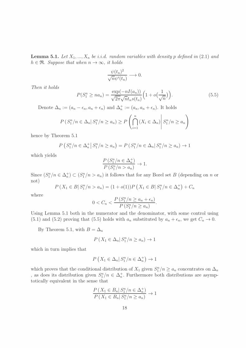
Lemma 5.1. Let X1, ..., Xn be i.i.d. random variables with density p defined in (2.1) andh ∈ R. Suppose that when n→ ∞, it holds

ψ(tn)2

√nψ′(tn)

−→ 0.

Then it holds

P (Sn1 ≥ nan) =

exp(−nI(an))√2π

√ntns(tn)

(1 + o

( 1√n

)). (5.5)

Denote ∆n := (an − ǫn, an + ǫn) and ∆+n := (an, an + ǫn). It holds

P (Sn1 /n ∈ ∆n|Sn

1 /n ≥ an) ≥ P

(n⋂

i=1

(Xi ∈ ∆n)

∣∣∣∣∣Sn1 /n ≥ an

)

hence by Theorem 5.1

P(Sn1 /n ∈ ∆+

n

∣∣Sn1 /n ≥ an

)= P (Sn

1 /n ∈ ∆n|Sn1 /n ≥ an) → 1

which yieldsP (Sn

1 /n ∈ ∆+n )

P (Sn1 /n > an)

→ 1.

Since (Sn1 /n ∈ ∆+

n ) ⊂ (Sn1 /n > an) it follows that for any Borel set B (depending on n or

not)P (X1 ∈ B|Sn

1 /n > an) = (1 + o(1))P(X1 ∈ B|Sn

1 /n ∈ ∆+n

)+ Cn

where

0 < Cn <P (Sn

1 /n ≥ an + ǫn)

P (Sn1 /n ≥ an)

.

Using Lemma 5.1 both in the numerator and the denominator, with some control using(5.1) and (5.2) proving that (5.5) holds with an substituted by an + ǫn, we get Cn → 0.

By Theorem 5.1, with B = ∆n

P (X1 ∈ ∆n|Sn1 /n ≥ an) → 1

which in turn implies that

P(X1 ∈ ∆n|Sn

1 /n ∈ ∆+n

)→ 1

which proves that the conditional distribution of X1 given Sn1 /n ≥ an concentrates on ∆n

, as does its distribution given Sn1 /n ∈ ∆+

n . Furthermore both distributions are asymp-totically equivalent in the sense that

P (X1 ∈ Bn|Sn1 /n ∈ ∆+

n )

P (X1 ∈ Bn|Sn1 /n ≥ an)

→ 1

18

for all sequence of Borel sets Bn such that

lim infn→∞

P (X1 ∈ Bn|Sn1 /n ≥ an) > 0.

.

We now prove Theorem 5.2.For a Borel set B = Bn it holds

PAn(B) =

∫ ∞

an

Pv(B)p (Sn1 /n = v|Sn

1 /n > an) dv

=1

P (Sn1 /n > an)

∫ ∞

an

Pv(B)p (Sn1 /n = v) dv

= (1 + o(1))1

P (Sn1 /n ∈ ∆+

n )

∫ ∞

an

Pv(B)p (Sn1 /n = v) dv

= (1 + o(1))1

P (Sn1 /n ∈ ∆+

n )

∫ an+ǫn

an

Pv(B)p (Sn1 /n = v) dv

+ (1 + o(1))1

P (Sn1 /n ∈ ∆+

n )

∫ ∞

an+ǫn

Pv(B)p (Sn1 /n = v) dv

= (1 + o(1))

∫ an+ǫn

an

Pv(B)p(Sn1 /n = v|Sn

1 /n ∈ ∆+n

)dv

+ (1 + o(1))1

P (Sn1 /n ∈ ∆+

n )

∫ ∞

an+ǫn

Pv(B)p (Sn1 /n = v) dv

= (1 + o(1))Pan+θnǫn(B)

+ (1 + o(1))1

P (Sn1 /n ∈ ∆+

n )

∫ ∞

an+ǫn

Pv(B)p (Sn1 /n = v) dv

= (1 + o(1))Pan+θnǫn(B) + Cn

for some θn in (0, 1) . The term Cn is less than P (Sn1 /n > an + ǫn)/P (S

n1 /n > an) which

tends to 0 as n tends to infinity, under (5.1) and (5.2), using Lemma 5.1.Hence when Bn is such that lim infn→∞ Pan+θnǫn(Bn) > 0 using Theorem 4.3 it holds,

since a′n := an + θnǫn satisfies (4.3)

PAn(Bn) = (1 + o(1))Gan+θnǫn(Bn). (5.6)

It remains to prove that

Gan+θnǫn(Bn) = (1 + o(1))Gan(Bn). (5.7)

Make use of (4.9) to prove the claim. Define t through m(t) = an and t′ throughm(t′) = a′n. It is enough to obtain

s(t) = (1 + o(1)) s(t′) (5.8)

19

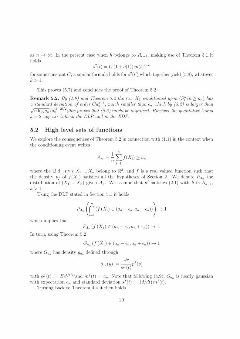
as n → ∞. In the present case when h belongs to Rk−1, making use of Theorem 3.1 itholds

s2(t) = C (1 + o(1))m(t)2−k

for some constant C; a similar formula holds for s2(t′) which together yield (5.8), whateverk > 1.

This proves (5.7) and concludes the proof of Theorem 5.2.

Remark 5.2. By (4.9) and Theorem 5.2 the r.v. X1 conditioned upon (Sn1 /n ≥ an) has

a standard deviation of order Ca2−kn , much smaller than ǫn which by (5.2) is larger than√n log an/a

(k−2)/2n ;this proves that (5.3) might be improved. However the qualitative bound

k = 2 appears both in the DLP and in the EDP.

5.2 High level sets of functions

We explore the consequences of Theorem 5.2 in connection with (1.1) in the context whenthe conditioning event writes

An :=1

n

n∑

i=1

f(Xi) ≥ an

where the i.i.d. r.v’s X1, .., Xn belong to Rd, and f is a real valued function such that

the density pf of f(X1) satisfies all the hypotheses of Section 2. We denote PAnthe

distribution of (X1, .., Xn) given An. We assume that pf satisfies (2.1) with h in Rk−1,k > 1.

Using the DLP stated in Section 5.1 it holds

PAn

(n⋂

i=1

(f (Xi) ∈ (an − ǫn, an + ǫn))

)→ 1

which implies thatPAn

(f (X1) ∈ (an − ǫn, an + ǫn)) → 1.

In turn, using Theorem 5.2

Gan (f (X1) ∈ (an − ǫn, an + ǫn)) → 1

where Gan has density gan defined through

gan(y) :=ety

φf(t)pf (y)

with φf (t) := Eetf(X)and mf (t) = an. Note that following (4.9), Gan is nearly gaussianwith expectation an and standard deviation sf(t) := (d/dt)mf (t).

Turning back to Theorem 4.4 it then holds

20

Theorem 5.1. When the above hypotheses hold let an satisfies

lim infn→∞

log g(an)

logn> δ

with h in Rk−1, k > 1 and

gan(x) :=etf(x)

φf(t)p(x)

where mf(t) = an . Then there exists a sequence ǫn satisfying limn→∞ ǫn/n = 0 suchthat a r.v. X in R

d with density gan is a solution of the inequation

an − ǫn < f(x) < an + ǫn

with probability 1 as n→ ∞. The sequence ǫn satisfies

limn→∞

n log anak−2n ǫ2n

= 0.

6 Appendix

6.1 Proof of Lemma 4.4

Case 1: if h ∈ Rβ. By Theorem 3.1, it holds s2 ∼ ψ′(t) with ψ(t) ∼ t1/βl1(t), where l1 issome slowly varying function. It also holds ψ′(t) = 1/h

′(ψ(t)

); therefore

1

s2∼ h

′(ψ(t)

)= ψ(t)β−1l0

(ψ(t)

)(β + ǫ

(ψ(t)

))

∼ βt1−1/βl1(t)β−1l0

(ψ(t)

)= o(t),

which implies that for any u ∈ Ku

s= o(t).

It follows that

s2 (t+ u/s)

s2∼ ψ′(t + u/s)

ψ′(t)=

ψ(t)β−1l0(ψ(t)

)(β + ǫ

(ψ(t)

))(ψ(t+ u/s)

)β−1l0(ψ(t + u/s)

)(β + ǫ

(ψ(t+ u/s)

))

∼ ψ(t)β−1

ψ(t + u/s)β−1∼ t1−1/βl1(t)

β−1

(t+ u/s)1−1/βl1(t+ u/s)β−1−→ 1.

21

Case 2: if h ∈ R∞. Then we have ψ(t) ∈ R0; hence it holds

1

st∼ 1

t√ψ′(t)

=

√1

tψ(t)ǫ(t)−→ 0.

Hence for any u ∈ K, we get as n→ ∞u

s= o(t),

thus using the slowly varying propriety of ψ(t) we have

s2 (t + u/s)

s2∼ ψ′(t+ u/s)

ψ′(t)=ψ(t+ u/s)ǫ(t+ u/s)

t + u/s

t

ψ(t)ǫ(t)

∼ ǫ(t+ u/s)

ǫ(t)=ǫ(t) +O

(ǫ′(t)u/s

)

ǫ(t)−→ 1,

where we used a Taylor expansion in the second line. This completes the proof.

6.2 Proof of Lemma 5.1

For the density p defined in (2.1), we show that g is convex when x is large. If h ∈ Rβ, itholds for x large

g′′

(x) = h′

(x) =h(x)

x

(β + ǫ(x)

)> 0.

If h ∈ R∞, its reciprocal function ψ(x) belongs to R0. Set x := ψ(u); for x large

g′′

(x) = h′

(x) =1

ψ′(u)=

u

ψ(u)ǫ(u)> 0,

where the inequality holds since ǫ(u) > 0 under condition (2.7), for large u. Therefore gis convex for large x .

Therefore, the density p with h ∈ R satisfies the conditions of Jensen’s Theorem 6.2.1([12]). A third order Edgeworth expansion in formula (2.2.6) of ([12]) yields

P (Sn1 ≥ nan) =

Φ(tn)n exp(−ntnan)√ntns(tn)

(B0(λn) +O

( µ3(tn)

6√ns3(tn)

B3(λn))), (6.1)

where λn =√ntns(tn), and B0(λn) and B3(λn) are defined by

B0(λn) =1√2π

(1− 1

λ2n+ o(

1

λ2n)), B3(λn) ∼ − 3√

2πλn.

22

We show that, as an → ∞,1

λ2n= o

(1

n

). (6.2)

Since n/λ2n = 1/(t2ns2(tn)), (6.2) is equivalent to show that

t2ns2(tn) −→ ∞. (6.3)

By Theorem 3.1, m(tn) ∼ ψ(tn) and s2(tn) ∼ ψ′(tn); this entails that tn ∼ h(an).

If h ∈ Rβ, notice that

ψ′(tn) =1

h′(ψ(tn))=

ψ(tn)

h(ψ(tn)

)(β + ǫ(ψ(tn))

) ∼ an

h(an)(β + ǫ(ψ(tn))

) .

holds. Hence we have

t2ns2(tn) ∼ h(an)

2 an

h(an)(β + ǫ(ψ(tn))

) =anh(an)

β + ǫ(ψ(tn))−→ ∞.

If h ∈ R∞, then ψ(tn) ∈ R0, it follows that

t2ns2(tn) ∼ t2n

ψ(tn)ǫ(tn)

tn= tnψ(tn)ǫ(tn) −→ ∞,

where the last step holds from condition (2.7). We have shown (6.2). Therefore

B0(λn) =1√2π

(1 + o

(1

n

)).

By (6.3), λn goes to ∞ as an → ∞, which implies further that B3(λn) → 0. On theother hand, by Theorem 3.1 , µ3/s

3 → 0. Hence we obtain from (6.1)

P (Sn1 ≥ nan) =

Φ(tn)n exp(−ntnan)√2πntns(tn)

(1 + o

(1√n

)),

which together with (5.4) proves the claim.

References

[1] Barndorff-Nielsen, O. Information and exponential families in statistical theory. Wi-ley Series in Probability and Mathematical Statistics. John Wiley & Sons, Ltd.,Chichester, 1978. ix+238 pp.

[2] Bingham, N.H., Goldie, C.M., Teugels, J.L. “Regular Variation,” Cambridge Univer-sity Press, Cambridge, (1987).

23

[3] Bhattacharya, R. N., Rao, Ranga R., “Normal approximation and asymptotic ex-pansions,” Society for Industrial and Applied Mathematics, Philadelphia, (2010).

[4] Broniatowski, M.,Cao, Z. Light tails: All summands are large when the empiricalmean is large. [hal-00813262] (2013).

[5] Broniatowski, M.,Cao, Z. A conditional limit theorem for random walks under ex-treme deviation. [hal-00713053] (2012).

[6] Broniatowski, M. and Caron, V. Long runs under a conditional limit distribution.[arXiv:1202.0731] (2012).

[7] Cattiaux, P. Gozlan, N. Deviations bounds and conditional principles for thin sets.Stochastic Process. Appl. 117 , no. 2, 221–250, (2007).

[8] Dembo, A. and Zeitouni, O. “Refinements of the Gibbs conditioning principle,”Probab. Theory Related Fields 104 1¨C14, (1996).

[9] Diaconis, P., Freedman, D. “Conditional Limit Theorems for Exponential Familiesand Finite Versions of de Finetti’s Theorem,” Journal of Theoretical Probability, Vol.1, No. 4, (1988).

[10] Feller, W. “An introduction to probability theory and its applications,” Vol. 2, secondedition, John Wiley and Sons Inc., New York, (1971).

[11] Sornette, D. Critical phenomena in natural sciences, Springer series in Synergetics,2d Edition (2006).

[12] Jensen, J. L. “Saddlepoint approximations,” Oxford Statistical Science Series, 16.Oxford Science Publications. The Clarendon Press, Oxford University Press, NewYork, (1995).

[13] Juszczak, D., Nagaev, A. V. “Local large deviation theorem for sums of i.i.d. ran-dom vectors when the Cramer condition holds in the whole space,” Probability andMathematical Statistics, Vol. 24, (2004), pp. 297-320.

24