light emission and optical interactions in nanoscale environments · 2019-08-03 · at the heart of...

Chapter 8

Light emission and optical

interactions in nanoscale

environments

The scope of this chapter is to discuss optical interactions between nanoscale systems

and the properties of the emitted radiation. This is different to Chapter ?? where we

considered the focusing and confinement of free propagating radiation. To link the

two topics it is also necessary to understand how focused light interacts with nanoscale

matter. This is a difficult task since it depends on the particular material properties,

the shape of the investigated objects and also on the strength of interaction. Never-

theless, there are issues that can be discussed from a more or less general point of view.

At the heart of nano-optics are light-matter interactions on the nanometer scale.

Optical interactions with nanoscale matter are encountered in various fields of re-

search. For example, the activity of proteins and other macromolecules is followed

by optical techniques, optically excited single molecules are used to probe their nano-

environment and optical interactions with semiconductor nanostructures (quantum

wells/wires/dots) are actively investigated because of their technological promise as

nanocomposite materials or quantum coherent devices. Furthermore, various nano-

metric structures are encountered in near-field optics as tiny light sources.

To rigorously understand light-matter interactions we need to invoke quantum

electrodynamics (QED). There are many textbooks that provide a good understand-

ing of optical interactions with atoms or molecules and we expecially recommend the

books in Refs. [1-3]. Since nanometer scale structures are often too complex to be

solved rigorously by QED we prefer to stick to classical theory and invoke the results

of QED in a phenomenological way. Of course, the results obtained in this way have

to be validated, but as long as there is no experimental contradiction we are save to

1

2 CHAPTER 8. LIGHT EMISSION AND OPTICAL INTERACTIONS

use this approach. A classical description is often more intuitive because of its simpler

formalism but also because it is closer to our perception.

8.1 The multipole expansion

In this section we will consider an arbitrary ‘piece of matter’ which is small compared

to the wavelength of light and which we will designate by particle. Although small

compared to the wavelength, this particle consists of many atoms or molecules. On

a macroscopic scale the charge density ρ and current density j can be treated as con-

tinuous functions of position. However, atoms and molecules are made of discrete

charges which are spatially separated. Thus, the microscopic structure of matter is

not considered in the macroscopic Maxwell equations. The macroscopic fields are

local spatial averages over microscopic fields.

In order to derive the potential energy for a microscopic system we have to give up

the definitions of the electric displacement D and the magnetic field H and consider

only the field vectors E and B in the empty space between a set of discrete charges qn.

We thus replace D= εoE and B=µoH in Maxwell’s equations [c.f. Eqs. (??)- (??)]

and set

ρ(r) =∑

n

qnδ[r − rn] , (8.1)

j(r) =∑

n

qnrnδ[r − rn] , (8.2)

rrn

qn

V

Figure 8.1: In the microscopic picture, optical radiation interacts with the discrete

charges qn of matter. The collective response of the charges with coordinates rn can

be described by a multipole expansion with origin r.

8.1. THE MULTIPOLE EXPANSION 3

where rn denotes the position vector of the n-th charge and rn its velocity. The to-

tal charge and current of the particle is obtained by a volume integration over ρ and j.

To derive the polarization and magnetization of the charge distribution we consider

the total current density as defined in Eq. (??)

j =dP

dt+ ∇× M . (8.3)

We ignored the contribution of the source current js which generates the incident field

Einc since it is not part of the considered particle. Furthermore, we incorporated the

conduction current jc into the polarization current. To solve for P we apply the

operator ∇· to both sides of Eq. (8.3). The last term on the right side vanishes

because of ∇·∇×=0 and the term on the left can be related to the time derivative of

the charge density through the continuity equation for charge (??). We then obtain

ρ = −∇ · P . (8.4)

If the particle is not charge neutral we need to add the net charge density to the right

side. Using Eq. (8.1) for the charge density it is possible to solve for P as [1]

P(r) =∑

n

qnrn

∫ 1

0

δ[r − srn] ds . (8.5)

Together with the current density in Eq. (8.2) this expression can be introduced into

Eq. (8.3). It is then possible to solve for M as [1]

M(r) =∑

n

qnrn×rn

∫ 1

0

sδ[r − srn] ds . (8.6)

To calculate the potential energy of the particle in the incident field we first con-

sider fixed charges, i.e. the charge distribution is not induced by the incident field.

Instead, the charge distribution is determined by the atomic and interatomic poten-

tials. Of course, the particle is polarizable but for the moment we consider this to

be a secondary effect. The important point is that on a microscopic scale the parti-

cle does have a permanent polarization and magnetization. On a macroscopic scale

it can loose this permanent magnetization and polarization because the microscopic

properties get averaged out. Thus, the importance of permanent polarization and

magnetization depends on the size and properties of the particle. This is what makes

the mesoscopic size range so challenging.

We now consider the interaction between a discrete charge distribution and an

electromagnetic field. The incident field in the absence of the charge distribution is

denoted as Einc. The electric potential energy of the permanent microscopic charge

distribution is determined as [4]

VE = −∫

V

P ·Einc dV = −∑

n

qn

∫ 1

0

rn ·Einc(srn) ds . (8.7)


Next, we expand the electric field Einc in a Taylor series with origin at the center of

the particle. For convenience we choose this origin at r=0 and obtain

Einc(srn) = Einc(0) + [srn ·∇]Einc(0) +1

2![srn ·∇]2Einc(0) + . . . (8.8)

This expansion can now be inserted into Eq. (8.7) and the integration over s can be

carried out. Then, the electrical potential energy expressed in terms of the multipole

moments of the charges becomes

VE = −∑

n

qnrn ·Einc(0) −∑

n

qn

2!rn ·[rn ·∇]Einc(0) −

∑

n

qn

3!rn ·[rn ·∇]2Einc(0) − . . .

(8.9)

The first term is recognized as the electric dipole interaction

V(1)

E = −µ · Einc(0) , (8.10)

with the electric dipole moment defined as

µ =∑

n

qnrn . (8.11)

The next higher term in Eq. (8.9) is the electric quadrupole interaction which can be

written as

V(2)

E = −[↔

Q ∇] ·Einc(0) , (8.12)

with the electric quadrupole moment defined as

↔

Q=1

2

∑

n

qnrnrn , (8.13)

where rnrn denotes the outer product. Therefore,↔

Q becomes a tensor of rank two.∗

Since ∇·Einc = 0 we can subtract any multiple of ∇·Einc from Eq. (8.12). We can

therefore rewrite Eq. (8.12) as

V(2)

E = −1

2[(

↔

Q −A↔

I )∇] · Einc(0) , (8.14)

with an arbitrary constant A which commonly is chosen as A=(1/3) |rn|2 because it

generates a traceless quadrupole moment. Thus, we can also define the quadrupole

moment as↔

Q=1

2

∑

n

qn

[

rnrn −↔

I

3|rn|2

]

. (8.15)

We avoid writing down the next higher multipole orders but we note that the rank of

every next higher multipole increases by one.

∗If we denote the cartesian components of rn by (xn1, xn2

, xn3) we can write Eq. (8.12) as

V(2)E

= −(1/2)∑

i,j

[∑

nqnxnixnj

]

[∂/∂xi Ej(0)].

8.1. THE MULTIPOLE EXPANSION 5

The dipole interaction is determined by the electric field at the center of the charge

distribution whereas the quadrupole interaction is defined by the electric field gra-

dients at the center. Thus, if the electric field is sufficiently homogeneous over the

dimensions of the particle, the quadrupole interaction vanishes. This is why in small

systems of charge, such as atoms or molecules, often only the dipole interaction is con-

sidered. This dipole approximation leads to the standard selection rules encountered in

optical spectroscopy. However, the dipole approximation is not necessarily sufficient

for nanoscale particles because of the larger size compared to an atom. Furthermore,

if the particle interacts with an optical near-field it will experience strong field gra-

dients. This increases the importance of the quadrupole interaction and modifies the

standard selection rules. Thus, the strong field gradients encountered in near-field

optics have the potential to excite usually forbidden transitions in larger quantum

systems and thus extend the capabilities of optical spectroscopy.

A similar multipole expansion can be performed for the magnetic potential energy

VM . The lowest order term is the magnetic dipole interaction

V(1)M = −md ·Binc(0) , (8.16)

with the magnetic dipole moment defined as

md =∑

n

(qn/2mn) rn × (mnrn) . (8.17)

The magnetic moment is often expressed in terms of the angular momenta In =

mnrn×rn, where mn denotes the mass of the n-th particle. We avoid deriving higher

order magnetic multipole terms since the procedure is analogous to the electric case.

So far we considered the polarization and magnetization of a charge distribution

that is not affected by the incident electromagnetic field. However, it is clear that the

incident radiation will act on the charges and displace them from their unperturbed

positions. This gives rise to an induced polarization and magnetization. The interac-

tion of the incident field Einc with the particle causes a change dP in the polarization

P. The change in the electric potential energy dVE due to this interaction is

dVE = −∫

V

Einc · dP dV . (8.18)

To calculate the total induced electric potential energy VE,ind we have to integrate

dVE over the polarization range Pp ..Pp+i, where Pp and Pp+i are the initial value

and final values of the polarization. We now assume that the interaction between the

field and the particle is linear so we can write P= εoχEinc. In this case we find for

the total differential d(P · Einc)

d(P ·Einc) = Einc · dP + P · dEinc = 2Einc · dP , (8.19)


and the induced potential energy becomes

VE,ind = −1

2

∫

V

[

∫ Pp+i

Pp

d(P· Einc)

]

dV . (8.20)

Using Pp+i =Pp+Pi we finally obtain

VE,ind = −1

2

∫

V

Pi ·Einc dV . (8.21)

This result states that the induced potential energy is smaller than the permanent

potential energy by a factor 1/2. The other 1/2 portion is related to the work needed

to build up the polarization from zero to Pi. For Pi >0 regions of high electric fields

cause an attracting force on polarizable objects (laser tweezers).

A similar derivation can be performed for the induced magnetization Mi and

its associated energy. The interesting outcome is that objects with Mi > 0 are re-

pelled from regions of high magnetic fields. This finding underlies the phenomenon of

eddy-current damping. However, at optical frequencies induced magnetizations are

practically zero.

8.2 The classical particle-field Hamiltonian

So far we have been concerned with the potential energy of a particle in an external

electromagnetic field. However, for a fundamental understanding of the interaction

of a particle with the electromagnetic field we require to know the total energy of the

system consisting of particle and field. This energy remains conserved; the particle

can borrow energy from the field (absorption) or it can donate energy to it (emission).

The total energy corresponds to the classical Hamiltonian H which constitutes the

Hamiltonian operator H encountered in quantum mechanics. For particles consisting

of many charges, the Hamiltonian soon becomes a very complex function: it depends

on the mutual interaction between the charges, their kinetic energies and the exchange

of energy with the external field.

To understand the interaction between a particle and an electromagnetic field

we first consider a single point-like particle with mass m and charge q. Later we

generalize the situation to systems consisting of multiple charges and with finite size.

The Hamiltonian for a single charge in an electromagnetic field is found by first

deriving a Lagrangian function L(r, r) which satisfies the Lagrange-Euler equation

d

dt

(

∂L

∂q

)

− ∂L

∂q= 0 , q=x, y, z . (8.22)

8.2. THE CLASSICAL PARTICLE-FIELD HAMILTONIAN 7

Here, q = (x, y, z) and q = (x, y, z) denote the coordinates of the charge and the ve-

locities, respectively.† To determine L, we first consider the (nonrelativistic) equation

of motion for the charge

F =d

dt[mr] = q (E + r × B) , (8.23)

and replace E and B by the vector potential A and scalar potential φ according to

E(r, t) = − ∂

∂tA(r, t) −∇φ(r, t) (8.24)

B(r, t) = ∇× A(r, t) . (8.25)

Now we consider the vector-components of Eq. (8.23) separately. For the x-component

we obtain

d

dt[mx] = −q

[

∂φ

∂x+

∂Ax

∂t

]

+ q

[

y

(

∂Ay

∂x− ∂Ax

∂y

)

− z

(

∂Ax

∂z− ∂Az

∂x

)]

(8.26)

=∂

∂x[−qφ + q (Axx + Ay y + Az z)] − q

[

∂Ax

∂t+ x

∂Ax

∂x+ y

∂Ay

∂y+ z

∂Az

∂z

]

.

Identifying the last expression in brackets with dAx/dt (total differential) and rear-

ranging terms, the equation above can be written as

d

dt[mx + qAx] − ∂

∂x[−qφ + q (Axx + Ay y + Az z)] = 0 . (8.27)

This equation has almost the form of the Lagrange-Euler equation (8.22). Therefore,

we seek a Lagrangian of the form

L = −qφ + q (Axx + Ay y + Az z) + f(x, x) , (8.28)

with ∂f/∂x = 0. With this choice, the first term in Eq. (8.22) leads to

d

dt

(

∂L

∂q

)

=d

dt

[

qAx +∂f

∂x

]

. (8.29)

This expression has to be identical with the first term in Eq. (8.27) which leads to

∂f/∂x = mx. The solution f(x, x) = mx2/2 can be substituted into Eq. (8.28) and,

after generalizing to all degrees of freedom, we finally obtain

L = −qφ + q (Axx + Ay y + Az z) +1

2m

(

x2 + y2 + z2)

, (8.30)

which can be written as

L = −qφ + qv ·A +m

2v ·v . (8.31)

†It is a convention of the Hamiltonian formalism to designate the generalized coordinates by the

symbol q. Here, it should not be confused with the charge q.


To determine the Hamiltonian H we first calculate the the canonical momentum

p = (µx, µy, µz) conjugate to the coordinates q = (x, y, z) according to pi = ∂L/∂qi.

The canonical momentum turns out to be

p = mv + qA , (8.32)

which is the sum of mechanical momentum mv and field momentum qA. According

to Hamiltonian mechanics, the Hamiltonian is derived from the Lagrangian according

to

H(q,p) =∑

i

[pi qi − L(q, q)] , (8.33)

in which all the velocities qi have to be expressed in terms of the coordinates qi and

conjugate momenta pi. This is easily done by using Eq. (8.32) as qi = pi/m− qAi/m.

Using this substitution in Eqs. (8.30) and (8.33) we finally obtain

H =1

2m[p− qA]

2+ qφ . (8.34)

This is the Hamiltonian of a free charge q with mass m in an external electromag-

netic field. The first term renders the kinetic mechanical energy and the second term

the potential energy of the charge. Notice, that the derivation of L and H is inde-

pendent of gauge, i.e. we did not imply any condition on ∇·A. Using Hamilton’s

canonical equations qi =∂H/∂pi and pi =−∂H/∂qi it is straightforward to show that

the Hamiltonian in Eq. (8.34) reproduces the equations of motion stated in Eq. (8.23).

The Hamiltonian of Eq. (8.34) is not yet the total Hamiltonian Htot of the system

“charge+field” since we did not include the energy of the electromagnetic field. Fur-

thermore, if the charge is interacting with other charges, as in the case of an atom or a

molecule, we must take into account the interaction between the charges. In general,

the total Hamiltonian for a system of charges can be written as

Htot = Hparticle + Hrad + Hint . (8.35)

Here, Hrad is the Hamiltonian of the radiation field in the absence of the charges and

Hparticle is the Hamiltonian of the system of charges (particle) in the absence of the

electromagnetic field. The interaction between the two systems is described by the

interaction Hamiltonian Hint. Let us determine the individual contributions.

The particle Hamiltonian Hparticle is determined by a sum of the kinetic energies

pn ·pn/(2mn) of the N charges and the potential energies V (rm, rn) between the

charges (intramolecular potential), i.e.,

Hparticle =∑

n,m

[

pn ·pn

2mn+ V (rm, rn)

]

, (8.36)

8.2. THE CLASSICAL PARTICLE-FIELD HAMILTONIAN 9

where the n-th particle is specified by its charge qn, mass mn, and coordinate rn.

Notice, that V (rm, rn) is determined in the absence of the external radiation field.

This term is solely due to the Coulomb interaction between the charges. Hrad is

defined by integrating the electromagnetic energy density W of the radiation field

[Eq. (??)] over all space as‡

Hrad =1

2

∫

[

εoE2 + µ−1

o B2]

dV , (8.37)

where E2 = |E|2 and B2 = |B|2. It should be noted, that the inclusion of Hrad is essen-

tial for a rigorous quantum electrodynamical treatment of light-matter interactions.

This term ensures that the system consisting of particles and fields is conservative; it

permits the interchange of energy between the atomic states and the states of the radi-

ation field. Spontaneous emission is a direct consequence of the inclusion of Hrad and

cannot be derived by semiclassical calculations in which Hrad is not included. Finally,

to determine Hint we first consider each charge separately. Each charge contributes

to Hint a term which can be derived from Eq. (8.34) as

H − p·p2m

= − q

2m[p·A + A·p] +

q2

2mA·A + qφ . (8.38)

Here, we subtracted the kinetic energy of the charge from the classical ‘particle-field’

Hamiltonian since this term is already included in Hparticle. Using p·A = A·p and

then summing the contributions of all N charges in the system we can write Hint as§

Hint =∑

n

[

− qn

mnA(rn, t)·pn +

q2n

2mnA(rn, t)·A(rn, t) + qnφ(rn, t)

]

. (8.39)

In the next section we will show that Hint can be expanded into a multipole series

similar to our previous results for VE and VM .

8.2.1 Multipole expansion of the interaction Hamiltonian

The Hamiltonian expressed in terms of the vector potential A and scalar potential

φ is not unique. This is caused by the freedom of gauge, i.e. if the potentials are

replaced by new potentials A, φ according to

A → A + ∇χ and φ → φ − ∂χ/∂t , (8.40)

‡This integration leads necessarily to an infinite result which caused difficulties in the development

of the quantum theory of light. Renormalization procedures are needed to overcome these problems.§In quantum mechanics, the canonical momentum p is converted to an operator according to

p → −ih∇ (Jordan rule) which turns also Hint into an operator. p and A commute only if the

Coulomb gauge (∇·A=0) is adopted.


with χ(r, t) being an arbitrary gauge function, Maxwell’s equations remain unaffected.

This is easily seen by introducing the above substitutions in the definitions of A and

φ [Eqs. (8.24) and (8.25)]. To remove the ambiguity caused by the freedom of gauge

we need to express Hint in terms of the original fields E and B. To do this, we

first expand the electric and magnetic fields in a Taylor series with origin r= 0 [c.f.

Eq. (8.8)]

E(r) = E(0) + [r·∇]E(0) +1

2![r·∇]2E(0) + . . . (8.41)

B(r) = B(0) + [r·∇]B(0) +1

2![r·∇]2B(0) + . . . , (8.42)

and introduce these expansions in the definitions for A and φ [Eqs. (8.24) and (8.25)].

The task is now to find an expansion of A and φ in terms of E and B such that the

left and right hand sides of Eqs. (8.24) and (8.25) are identical. These expansions

have been determined by Barron and Gray as [6]

φ(r) = φ(0) −∞∑

i=0

r [r·∇]i

(i+1)!·E(0) , A(r) =

∞∑

i=0

[r·∇]i

(i+2) i!B(0) × r . (8.43)

Inserting into the expression for Hint in Eq. (8.39) leads to the so-called multipolar

interaction Hamiltonian

Hint = qtot φ(0, t) − µ ·E(0, t) − m ·B(0, t) − [↔

Q ∇] · E(0, t) − . . . , (8.44)

in which we used the following definitions

qtot =∑

n

qn, µ =∑

n

qnrn, m =∑

n

(qn/2mn) rn×pn,↔

Q=∑

n

(qn/2)rnrn ,

(8.45)

qtot is the total charge of the system, µ denotes the total electric dipole moment,

m the total magnetic dipole moment, and↔

Q the total electric quadrupole moment.

If the system of charges is charge neutral, the first term in Hint vanishes and we

are left with an expansion which looks very much like the former expansion of the

potential energy VE + VM . However, the two expansions are not identical! First, the

new magnetic dipole moment is defined in terms of the canonical momenta pn and

not by the mechanical momenta mnrn.¶ Second, the expansion of Hint contains a

term nonlinear in B(0, t) which is nonexistent in the expansion of VE + VM . The

nonlinear term arises from the term A · A of the Hamiltonian and is referred to as

the diamagnetic term. It reads as∑

n

(q2n/8mn) [rn × B(0, t)]

2. (8.46)

¶A gauge transformation also transforms the canonical momenta. Therefore, the canonical mo-

menta pn are different from the original canonical momenta pn.

8.3. THE RADIATING ELECTRIC DIPOLE 11

Our previous expressions for VE and VM have been derived by neglecting retarda-

tion and assuming weak fields. In this limit, the nonlinear term in Eq. (8.46) can

be neglected and the canonical momentum can be approximated by the mechanical

momentum.

The multipolar interaction Hamiltonian can easily be converted to an operator

by simply applying Jordan’s rule p → −ih∇ and replacing the fields E and B by

the corresponding electric and magnetic field operators. However, this is beyond the

present scope. Notice, that the Hamiltonian Hint in Eq. (8.44) is gauge independent.

The gauge affects Hint only when the latter is expressed in terms of A and φ but not

when it is represented by the original fields E and B. The first term in the multipolar

Hamiltonian of a charge neutral system is the dipole interaction which is identical to

the corresponding term in VE . In most circumstances, it is sufficiently accurate to

reject the higher terms in the multipolar expansion. This is especially true for farfield

interactions where the magnetic dipole and electric quadrupole interaction are roughly

two orders of magnitude weaker than the electric dipole interaction. Therefore, stan-

dard selection rules for optical transitions are based on the electric dipole interaction.

However, in strongly confined optical fields as encountered in near-field optics, higher-

order terms in the expansion of Hint can become important and the standard selection

rules can be violated. Finally, it should be noted, that the multipolar form of Hint

can also be derived from Eq. (8.39) by a unitary transformation [7]. This transfor-

mation, commonly referred to as the Power-Zienau-Woolley transformation, plays an

important role in quantum optics [3].

We have established that to first order any neutral system of charges (particle),

that is smaller than the wavelength of the interacting radiation, can be viewed as a

dipole. In the next section we will consider its radiating properties.

8.3 The radiating electric dipole

The current density due to a distribution of charges qn with coordinates rn and

velocities rn has been given in Eq. (8.2). We can develop this current density in a

Taylor series with origin ro which is typically at the center of the charge distribution.

If we keep only the lowest order term we find

j(r, t) =d

dtµ(t) δ[r − ro] , (8.47)

with the dipole moment

µ(t) =∑

n

qn[rn(t) − ro] . (8.48)

The dipole moment is identical with the definition in Eq. (8.11) for which we had ro =

0. We assume a harmonic time-dependence which allows us to write the current den-


sity as j(r, t)=Rej(r) exp(−iωt) and the dipole moment as µ(t)=Reµ exp(−iωt).Eq. (8.47 can then be written as

j(r) = −iωµ δ[r − ro] . (8.49)

Thus, to lowest order, any current density can be thought of as an oscillating dipole

with origin at the center of the charge distribution.

8.3.1 Electric dipole fields in a homogeneous space

In this section we will derive the fields of a dipole representing the current density

of a small charge distribution located in a homogeneous, linear and isotropic space.

The fields of the dipole can be derived by considering two oscillating charges q of

opposite sign, separated by an infinitesimal vector ds. In this physical picture the

dipole moment is given by µ= qds. However, it is more elegant to derive the dipole

fields using the Green’s function formalism developed in Section ??. There, we have

derived the so-called volume integral equations [c.f. Eqs. (??) and (??)]

E(r) = Eo + iωµµo

∫

V

↔

G (r, r′) j(r′) dV ′ , (8.50)

H(r) = Ho +

∫

V

[

∇×↔

G (r, r′)]

j(r′) dV ′ . (8.51)

↔

G denotes the dyadic Green’s function and Eo,Ho are the fields in the absence of the

current j. The integration runs over the source volume specified by the coordinate r′.

If we introduce the current from Eq. (8.49) into the last two equations and assume

that all fields are produced by the dipole we find

E(r) = ω2µµo

↔

G (r, ro)µ , (8.52)

H(r) = −iω[

∇×↔

G (r, ro)]

µ . (8.53)

Hence, the fields of an arbitrarily oriented electric dipole located at r=ro are deter-

mined by the Green’s function↔

G (r, ro). As mentioned earlier, each column vector of↔

G specifies the electric field of a dipole whose axis is aligned with one of the coordinate

axes. For a homogeneous space,↔

G has been derived as

↔

G (r, ro) =

[

↔

I +1

k2∇∇

]

G(r, ro) , G(r, ro) =exp(ik|r−ro|)

4π|r−ro|. (8.54)

where↔

I is the unit dyad and G(r, ro) the scalar Green’s function. It is straightforward

to calculate↔

G in the major three coordinate systems. In a Cartesian system↔

G can

be written as

↔

G (r, ro) =exp(ikR)

4πR

[(

1 +ikR − 1

k2R2

)

↔

I +3 − 3ikR − k2R2

k2R2

RR

R2

]

, (8.55)


where R is the absolute value of the vector R = r−ro and RR denotes the outer

product of R with itself. Eq. (8.55) defines a symmetric 3×3 matrix

↔

G =

Gxx Gxy Gxz

Gxy Gyy Gyz

Gxz Gyz Gzz

, (8.56)

which, together with Eqs. (8.52) and (8.53), determines the electromagnetic field of an

arbitrary electric dipole µ with Cartesian components µx, µy, µz. The tensor [∇×↔

G]

can be expressed as

∇×↔

G (r, ro) =exp(ikR)

4πR

k(

R×↔

I)

R

(

i − 1

kR

)

, (8.57)

where R×↔

I denotes the matrix generated by the cross-product of R with each column

vector of↔

I .

The Green’s function↔

G has terms in (kR)−1, (kR)−2 and (kR)−3. In the farfield,

for which R ≫ λ, only the terms with (kR)−1 survive. On the other hand, the

dominant terms in the near-field, for which R≪λ, are the terms with (kR)−3. The

terms with (kR)−2 dominate the intermediate field at R ≈ λ. To distinguish these

three ranges it is convenient to write↔

G =↔

GNF +↔

GIF +↔

GFF , (8.58)

where the near-field (GNF ), intermediate field (GIF ) and farfield (GFF ) Green’s

functions are given by

↔

GNF =exp(ikR)

4πR

1

k2R2

[

−↔

I + 3RR/R2]

, (8.59)

rϑ

ϕ

E

p

x

y

z

Figure 8.2: The fields of a dipole are most conveniently represented in a spherical

coordinate system (r, ϑ, ϕ) in which the dipole points along the z-axis (ϑ=0).


↔

GIF =exp(ikR)

4πR

i

kR

[↔

I − 3RR/R2]

, (8.60)

↔

GFF =exp(ikR)

4πR

[↔

I −RR/R2]

. (8.61)

Notice that the intermediate field is 90 out of phase with respect to the near- and

farfield.

Because the dipole is located in a homogeneous environment, all three dipole orien-

tations lead to fields which are identical upon suitable frame rotations. We therefore

choose a coordinate system with origin at r = ro and a dipole orientation along the

dipole axis, i.e. µ = |µ|nz (c.f. Fig. 8.2). It is most convenient to represent the

dipole fields in spherical coordinates r=(r, ϑ, ϕ) and in spherical vector components

E = (Er, Eϑ, Eϕ). In this system the field components Eϕ and Hr, Hϑ are identical

to zero and the only non-vanishing field components are

Er =|µ| cosϑ

4πεoε

exp(ikr)

rk2

[

2

k2r2− 2i

kr

]

, (8.62)

Eϑ =|µ| sin ϑ

4πεoε

exp(ikr)

rk2

[

1

k2r2− i

kr− 1

]

, (8.63)

0.2 0.5 1 2 5 10

1

10

100

1000

0.1

r-1

r-3

transverse field

0.2 0.5 1 2 5 10

1

10

100

1000

0.1

r-2

r-3

longitudinal field

field

ampli

tude

k r k r

Figure 8.3: Radial decay of the dipole’s transverse and longitudinal fields. The

curves correspond to the absolute value of the expressions in brackets of Eqs. (8.62)

and (8.63), respectively. While both the transverse and the longitudinal field con-

tribute to the near-field, only the transverse field survives in the farfield. Notice, that

the intermediate field with (kr)−2 does not really show up for the transverse field.

Instead the near-field dominates for (kr)<1 and the far-field for (kr)>1.


Hϕ =|µ| sin ϑ

4πεoε

exp(ikr)

rk2

[

− i

kr− 1

] √

εoε

µoµ. (8.64)

The fact that Er has no farfield term ensures that the field in the farfield is purely

transverse. Furthermore, since the magnetic field has no terms in (kr)−3 the near-

field is dominated by the electric field. Thus, close to the origin of the dipole the

magnetic field strength is much smaller than the electric field strength which justifies

a quasi-electrostatic consideration.

So far we have considered a dipole which oscillates harmonically in time, i.e. µ(t)=

Reµ exp(−iωt). Therefore, the electromagnetic field is monochromatic and oscil-

lates at the same frequency. Although it is possible to generate any time-dependence

by a superposition of monochromatic fields (Fourier transformation), it is of advan-

tage for ultrafast applications to have the full time dependence available. The fields

of a dipole µ(t) with arbitrary time dependence can be derived by using the time-

dependent Green’s function. In a non-dispersive medium it is easier to introduce the

explicit time dependence by using the substitutions

exp(ikr) kmµ = exp(ikr)

[

in

c

]m

(−iω)mµ →

[

in

c

]mdm

dtmµ

(

t− rn/c)

, (8.65)

where n denotes the (dispersionfree) index of refraction ‖ and (t−nr/c) is the retarded

time. With this substitution, the dipole fields read as

Er(t) =cosϑ

4πεoε

[

2

r3+

n

c

2

r2

d

dt

]

∣

∣µ(

t− rn/c)∣

∣ , (8.66)

‖A dispersion-free index of refraction different from one is an approximation since it violates

causality.

x 10’000

λλ/10

zz

Figure 8.4: Electric energy density outside a fictitious sphere enclosing a dipole µ =

µz . (a) Close to the dipole’s origin the field distribution is elongated along the dipole

axis (near-field). (b) At larger distances the field spreads transverse to the dipole axis

(farfield).


Eϑ(t) =sinϑ

4πεoε

[

1

r3+

n

c

1

r2

d

dt+

n2

c2

1

r

d2

dt2

]

∣

∣µ(

t− rn/c)∣

∣ , (8.67)

Hϕ(t) =sinϑ

4πεoε

√

εoε

µoµ

[

n

c

1

r2

d

dt+

n2

c2

1

r

d2

dt2

]

∣

∣µ(

t− rn/c)∣

∣ . (8.68)

We see that the farfield is generated by the acceleration of the charges which con-

stitute the dipole moment. Similarly, the intermediate field and the near-field are

generated by the speed and the position of the charges, respectively.

8.3.2 Dipole radiation

It can be shown (see Problem 8.3) that only the farfield of the dipole contributes to

the net energy transport. The Poynting vector S(t) associated with the farfield can

be calculated by retaining only the r−1 terms in the dipole fields. We obtain

S(t) = E(t) × H(t) =1

16π2εoε

sin2 ϑ

r2

n3

c3

[

d2

dt2

∣

∣µ(

t− rn/c)∣

∣

]2

nr . (8.69)

The radiated power P can be determined by integrating S(t) over a closed spherical

surface as

P (t) =

∫

∂V

S·n da =1

4πεoε

2 n3

3 c3

[

d2 |µ(t)|dt2

]2

, (8.70)

where we have shrunk the radius of the sphere to zero to get rid of the retarded time.

The average radiated power for a harmonically oscillating dipole turns out to be

P =|µ|2

4πεoε

n3ω4

3 c3, (8.71)

which could have been also calculated by integrating the time-averaged Poynting

vector 〈S〉=(1/2)ReE×H∗, E and H being the dipole’s complex field amplitudes

given by Eqs. (8.62)-(8.64). We find that the radiated power scales with the fourth

power of the frequency. To determine the normalized radiation pattern we calculate

the power P (ϑ, ϕ) radiated into an infinitesimal unit solid angle dΩ=sin ϑdϑdϕ and

divide by the total radiated power P

P (ϑ, ϕ)

P=

3

8πsin2ϑ . (8.72)

Most of the energy is radiated perpendicular to the dipole moment and there is no

radiation at all in direction of the dipole.

Although we have considered an arbitrary time-dependence for the dipole we will

restrict ourselves in the following to the time harmonic case. It is straightforward to

account for dispersion when working with time-harmonic fields and arbitrary time-

dependences can be introduced by using Fourier transforms.


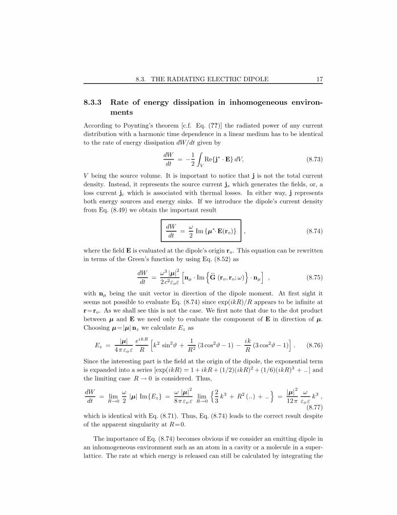
8.3.3 Rate of energy dissipation in inhomogeneous environ-

ments

According to Poynting’s theorem [c.f. Eq. (??)] the radiated power of any current

distribution with a harmonic time dependence in a linear medium has to be identical

to the rate of energy dissipation dW/dt given by

dW

dt= −1

2

∫

V

Rej∗ ·E dV, (8.73)

V being the source volume. It is important to notice that j is not the total current

density. Instead, it represents the source current js which generates the fields, or, a

loss current jc which is associated with thermal losses. In either way, j represents

both energy sources and energy sinks. If we introduce the dipole’s current density

from Eq. (8.49) we obtain the important result

dW

dt=

ω

2Im µ∗·E(ro) , (8.74)

where the field E is evaluated at the dipole’s origin ro. This equation can be rewritten

in terms of the Green’s function by using Eq. (8.52) as

dW

dt=

ω3 |µ|22c2εoε

[

nµ · Im

↔

G (ro, ro; ω)

· nµ

]

, (8.75)

with nµ being the unit vector in direction of the dipole moment. At first sight it

seems not possible to evaluate Eq. (8.74) since exp(ikR)/R appears to be infinite at

r=ro. As we shall see this is not the case. We first note that due to the dot product

between µ and E we need only to evaluate the component of E in direction of µ.

Choosing µ= |µ|nz we calculate Ez as

Ez =|µ|

4πεo ε

eikR

R

[

k2 sin2ϑ +1

R2(3 cos2ϑ − 1) − ik

R(3 cos2ϑ − 1)

]

. (8.76)

Since the interesting part is the field at the origin of the dipole, the exponential term

is expanded into a series [exp(ikR) = 1+ ikR + (1/2)(ikR)2 + (1/6)(ikR)3 + .. ] and

the limiting case R → 0 is considered. Thus,

dW

dt= lim

R→0

ω

2|µ| ImEz =

ω |µ|28πεo ε

limR→0

2

3k3 + R2 (..) + ..

=|µ|212π

ω

εo εk3 ,

(8.77)

which is identical with Eq. (8.71). Thus, Eq. (8.74) leads to the correct result despite

of the apparent singularity at R=0.

The importance of Eq. (8.74) becomes obvious if we consider an emitting dipole in

an inhomogeneous environment such as an atom in a cavity or a molecule in a super-

lattice. The rate at which energy is released can still be calculated by integrating the


Poynting vector over a surface enclosing the dipole emitter. However, to do this, we

need to know the electromagnetic field everywhere on the enclosing surface. Because

of the inhomogeneous environment, this field is not equal to the dipole field alone!

Instead, it is the self-consistent field, i.e. the field E generated by the superposition

of the dipole field Eo and the scattered field Es from the environment. Thus, to

determine the energy dissipated by the dipole we first need to determine the electro-

magnetic field everywhere on the enclosing surface. However, by using Eq. (8.74) we

can do the same job by only evaluating the total field at the dipole’s origin ro. It is

convenient to decompose the electric field at the dipole’s position as

E(ro) = Eo(ro) + Es(ro) , (8.78)

where Eo and Es are the primary dipole field and the scattered field, respectively.

Introducing Eq. (8.78) into Eq. (8.74) allows us to split the rate of energy dissipation

P =dW/dt into two parts. The contribution of Eo has been determined in Eq. (8.71)

and Eq. (8.77) as

Po =|µ|212π

ω

εoεk3 , (8.79)

which allows us to write for the normalized rate of energy dissipation

P

Po= 1 +

6πεo ε

|µ|21

k3Imµ∗ ·Es(ro) . (8.80)

Thus, the change of energy dissipation depends on the secondary field of the dipole.

This field corresponds to the dipole’s own field emitted at a former time. It arrives

at the position of the dipole after it has been scattered in the environment.

8.3.4 Radiation reaction

An oscillating charge produces electromagnetic radiation. This radiation not only

dissipates the energy of the oscillator but it also influences the motion of the charge.

This back-action is called radiation damping or radiation reaction. With the inclusion

of the reaction force Fr the equation of motion for an undriven harmonic oscillator

becomes

mr + ω2omr = Fr , (8.81)

where ω2om = c is the linear spring constant. According to Eq. (8.70) the average rate

of energy dissipation is

P (t) =1

4πεo

2

3 c3

[

d2 |µ(t)|dt2

]2

=q2 (r · r)6πεoc3

. (8.82)


Integrated over a certain time period T = [t1 .. t2], this term must be equal to the

work exerted on the oscillating charge by the radiation reaction force. Thus,

t2∫

t1

[

Fr · r +q2 (r · r)6πεoc3

]

dt = 0. (8.83)

After integrating the second term by parts we obtain

t2∫

t1

[

Fr · r − q2 (r· ···r)

6πεoc3

]

dt +q2 (r · r)6πεoc3

∣

∣

∣

t2

t1= 0 . (8.84)

For short time-intervals T → 0, the integrated term goes to zero and consequently

the remaining integrand has to vanish, i.e.

Fr =q2 ···

r

6πεoc3, (8.85)

which is the Abraham-Lorentz formula for the radiation reaction force. The equation

of motion (8.81) now becomes

r − q2

6πεoc3m

···r + ω2

or = 0 . (8.86)

Assuming that the damping introduced by the radiation reaction force is negligible,

the solution becomes r(t) = ro exp[−iωo t] and hence···r = −ω2

o r. Thus, for small

damping, we obtain

r + γor + ω2or = 0 , γo =

1

4πεo

2 q2 ω2o

3c3m. (8.87)

This equation corresponds to an undriven Lorentzian atom model with transition fre-

quency ωo and linewidth γo. A more rigorous derivation shows that radiation reaction

not only affects the damping of the oscillator due to radiation but also the oscillator’s

effective mass. This additional mass contribution is called the electromagnetic mass

and it is the source of many controversies [8].

Due to radiation damping the undriven oscillator will ultimately come to rest.

However, the oscillator interacts with the vacuum field which keeps the oscillator

alive. Consequently, a driving term accounting for the fluctuating vacuum field Eo

has to be added to the right hand side of Eq. (8.87). The fluctuating vacuum field

compensates the dissipation of the oscillator. Such fluctuation-dissipation relations

will be discussed in Chapter ??. In short, to preserve an equilibrium between the

oscillator and the vacuum, the vacuum must give rise to fluctuations if it takes energy

from the oscillator (radiation damping). It can be shown that spontaneous emission

is the result of both radiation reaction and vacuum fluctutions [8].


Finally, let us remark that radiation reaction is an important ingredient to obtain

the correct result for the optical theorem in the dipole limit [9], i.e. for a particle that

is described by a polarizability α. In this limit, an incident field polarizes the particle

and induces a dipole moment µ which in turn radiates a scattered field. According to

the optical theorem, the extinct power (sum of scattered and absorbed power) can be

expressed by the field scattered in the forward direction. However, it turns out that

in the dipole limit the extinct power is identical with the absorbed power and hence

light scattering is not taken into account! The solution to this dilemma is provided

by the radiation reaction term in Eq. (8.85) and is analyzed in more detail in Prob-

lem 8.5. In short, the particle not only interacts with the external driving field but

also with its own field causing a phase-lag between the induced dipole oscillation and

the driving electric field oscillation. This phase-lag recovers the optical theorem and

is responsible for light scattering in the dipole limit.

8.4 Spontaneous decay

Before Purcell’s analysis in 1946, spontaneous emission was considered a radiative

intrinsic property of atoms or molecules [10]. Purcell’s work established that the

spontaneous decay rate of a magnetic dipole placed in a resonant electronic device

can be enhanced compared to the free space decay rate. Thus, it can be inferred

that the environment in which the atoms are embedded modifies the radiative prop-

erties of the atoms. In order to experimentally observe this effect a physical device

with dimensions on the order of the emission wavelength λ is needed. Since most of

the atomic transitions occur in or near the visible spectral range, the modification of

spontaneous decay was not an obvious fact. Drexhage investigated the effect of planar

interfaces on the spontaneous decay rate of molecules [11] and the enhancement of

the atomic decay rates in a cavity was verified by Goy et al. [12]. Kleppner observed

that the decay of excited atoms can also be inhibited by a cavity [13]. Another novel

structure, the photonic crystal (optical structure with a periodic dielectric function)

was first conceived by Yablonovitch and John, as a system to control radiative prop-

erties [14, 15]. Photonic crystals exhibit forbidden photonic bandgaps which may

inhibit the decay of an excited atomic system. Related potential applications are

thresholdless lasers, perfect mirrors, wave guides bending light by 90 degrees without

loss, etc. [16]. Changes of molecular decay rates have also been observed in near-field

optical microscopy since molecules near optical probes experience a modified density

of states [17]. Recently, it was also demonstrated that non-radiative energy transfer

between adjacent molecules (Forster transfer) can be modified by an inhomogeneous

environment [18].

In the theory of atom-field interaction there are two physically distinctive regimes,

8.4. SPONTANEOUS DECAY 21

namely, the strong and weak coupling regimes. The two regimes are distinguished on

basis of the atom-field coupling constant which is estimated as

κ =µ

h

√

hωo

2εoV, (8.88)

where ωo is the atomic transition frequency, µ the dipole matrix element, and V the

volume of the cavity. Strong coupling satisfies the condition κ ≫ γcav, γcav being

the photon decay rate inside the cavity. In the strong coupling regime only quantum

electrodynamics (QED) can give an accurate description of atom-field interactions.

For example, the emission spectrum of an atom inside a cavity with a high qual-

ity factor (Q → ∞) exhibits two distinct peaks[19, 20]. On the other hand, in the

weak-coupling regime (κ ≪ γcav) it has been shown that QED and classical theory

give the same results for the modification of the spontaneous emission decay rate by

inhomogeneous environments. Classically, the modification of the spontaneous decay

rate is generated by the scattering of the atomic field in the environment, whereas

in the QED picture, the decay rate is partly stimulated by vacuum field fluctuations,

the latter being a function of the environment.

8.4.1 QED of spontaneous decay

In this section we derive the spontaneous emission rate γ for a two-level quantum

system located at r=ro. Spontaneous decay is a pure quantum effect and requires a

QED treatment. This section is intended to put classical treatments into the proper

context. We consider the combined ‘field+system’ states and calculate the transitions

from the excited state |i〉 with energy Ei to a set of final states |f〉 with identical

energies Ef (see Fig. 8.5). The final states differ only by the mode k of the radiation

field.∗∗ The derivation presented here is based on the Heisenberg picture. An equiv-

alent derivation is presented in Appendix ??.

According to Fermi’s Golden Rule γ is given by

γ =2π

h2

∑

f

∣

∣

∣〈f | HI |i〉

∣

∣

∣

2

δ(ωi − ωf ) (8.89)

where HI = −µ·E is the interaction Hamiltonian in the dipole approximation. Notice,

that all ωf are identical. Using the expression for HI we can substitute as follows∣

∣

∣〈f | HI |i〉

∣

∣

∣

2

= 〈f | µ · E |i〉∗ 〈f | µ · E |i〉 = 〈i| µ · E |f〉〈f | µ · E |i〉 . (8.90)

Let us represent the electric field operator E at r=ro as [2]

E =∑

k

[

E+k ak(t) + E−

k a†k(t)

]

, (8.91)

∗∗k is not to be confused with the wavevector. It is a label denoting a specific mode which in turn

is characterized by the polarization vector and the wavevector.


where

a†k(t) = a†

k(0) exp(iωkt), ak(t) = ak(0) exp(−iωkt) . (8.92)

Here, ak(0) and a†k(0) are the annihilation and creation operators, respectively. The

sum over k refers to summation over all modes. ωk denotes the frequency of mode

k. The spatially dependent complex fields E+k =(E−

k )∗ are the positive and negative

frequency parts of the complex field Ek. For a two-level atomic system with the

ground state |g〉 and the excited state |e〉, the dipole moment operator µ can be

written as

µ = µ[

r+ + r]

, with r+ = |e〉〈g| and r = |g〉〈e| . (8.93)

In this notation, µ is simply the transition dipole moment which is assumed to be

real, i.e. 〈g| µ |e〉 = 〈e| µ |g〉. Using the expressions for E and µ, the interaction

Hamiltonian takes on the form

−µ · E = −∑

k

µ ·[

E+k r+ak(t) + E−

k r a†k(t) + E+

k r ak(t) + E−k r+a†

k(t)]

. (8.94)

We now define the initial and final state of the combined system ‘field+atom’ as

|i〉 = |e, 0〉 = |e〉 |0〉 (8.95)

|f〉 =∣

∣g, 1ωk′⟩

= |f〉∣

∣1ωk′⟩

, (8.96)

| e,0⟩

| g,1ωk1⟩ | g,1ωk2

⟩ | g,1ωk3⟩ | g,1ωk

⟩

...

...

E

Ei

Ef

@ ωο

Figure 8.5: Transition from an initial state |i〉= |e, 0〉 to a set of final states |f〉=

|g, 1ωk〉. All the final states have the same energy. The difference of initial and final

energies is (Ei−Ef ) = hωo. The states are products of atomic states (|e〉 or |g〉) and

single-photon states (|0〉 or |1ωk〉). The number of distinct final single-photon

states is defined by the partial local density of states ρµ(ro, ωo), with ro being the

origin of the two-level system.


respectively. Here, |0〉 denotes the zero-photon state, and∣

∣1ωk′⟩

designates the

one-photon state associated with mode k′ and frequency ωo = (Ee−Eg)/h, Ee and

Eg being the energies of excited state and ground state, respectively. Thus, the final

states in Eq. (8.89) are associated with the different modes k′. Operating with µ · Eon state |i〉 leads to

µ · E |i〉 = µ ·∑

k

E−k eiωkt |g, 1ωk

〉 , (8.97)

where we used a†k(0) |0〉= |1ωk

〉. Operating with 〈f | gives

〈f | µ · E |i〉 = µ ·∑

k

E−k eiωkt

⟨

g, 1ωk′ | g, 1ωk

〉 , (8.98)

where we used ak(0) |1ωk〉=0. A similar procedure leads to

〈i| µ · E |f〉 = µ ·∑

k

E+k e−iωkt 〈g, 1ωk

∣

∣ g, 1ωk′⟩

. (8.99)

The matrix elements can now be introduced into Eq. (8.90) and Eq. (8.89). Ex-

pressing the sum over the final states as a sum over the modes k′ the transition rate

becomes

γ =2π

h2

∑

k

∑

k′′

[

µ ·E+k′′E

−k · µ

]

ei(ωk−ωk′′ )t × (8.100)

∑

k′

⟨

g, 1ωk′′

∣

∣ g, 1ωk′⟩ ⟨

g, 1ωk′ | g, 1ωk

〉 δ(ωk′ − ωo) .

Because of orthogonality, the only nonvanishing terms are those for which k′=k′′=k

which leads to the simple expression

γ =2π

h2

∑

k

[

µ · (E+k E−

k ) · µ]

δ(ωk − ωo) . (8.101)

Here, E+k E−

k denotes the outer product, i.e. the result is a 3×3 matrix. For later

purposes it is convenient to rewrite this expression in terms of normal modes uk

defined as

E+k =

√

hωk

2εouk, E−

k =

√

hωk

2εou∗

k . (8.102)

Because the delta function imposes ωk =ωo the decay rate can be written as

γ =2ω

3hεo|µ|2 ρµ(ro, ωo) , ρµ(ro, ωo) = 3

∑

k

[nµ ·(uku∗k)·nµ] δ(ωk − ωo) (8.103)

where we introduced the partial local density of states ρµ(ro, ωo) which will be dis-

cussed in the next section. The dipole moment has been decomposed as µ = µnµ


with nµ being the unit vector in direction of µ. The above equation for γ is our main

result. The delta-function in the expression suggests that we need to integrate over a

finite distribution of final frequencies. However, even for a single final frequency, the

apparent singularity introduced through δ(ωk − ωo) is compensated by the normal

modes whose magnitude tends to zero for a sufficiently large mode volume. In any

case, it is convenient to get rid of these singularities by representing ρµ(ro, ωo) in

terms of the Green’s function instead of normal modes.

8.4.2 Spontaneous decay and Green’s dyadics

We aim at deriving an important relationship between the normal modes uk and the

dyadic Green’s function↔

G. Subsequently, this relationship is used to express the

spontaneous decay rate γ and to establish an elegant expression for the local density

of states. While we suppressed the explicit position-dependence of uk in the previous

section for notational convenience, it is essential in the current context to carry all

the arguments along. The normal modes defined in the previous section satisfy the

wave-equation

∇×∇× uk(r, ωk) − ω2k

c2uk(r, ωk) = 0 (8.104)

and they fulfill the orthogonality relation∫

uk(r, ωk) · u∗k′(r, ωk′) d3r = δkk′ , (8.105)

where the integration runs over the entire mode volume. δkk′ is the Kronecker delta

and↔

I the unit dyad. We now expand the Green’s function↔

G in terms of the normal

modes as↔

G(r, r′; ω) =∑

k

Ak(r′, ω)uk(r, ωk) , (8.106)

where the vectorial expansion coefficients Ak have yet to be determined.

We recall the definition of the Green’s function [c.f. Eq. (??)]

∇×∇×↔

G (r, r′; ω) − ω2

c2

↔

G(r, r′; ω) =↔

I δ(r−r′) . (8.107)

To determine the coefficients Ak we substitute the expansion for↔

G and obtain

∑

k

Ak(r′, ω)

[

∇×∇× uk(r, ωk) − ω2

c2uk(r, ωk)

]

=↔

I δ(r−r′) . (8.108)

Using Eq. (8.104) we can rewrite the latter as

∑

k

Ak(r′, ω)

[

ω2k

c2− ω2

c2

]

uk(r, ωk) =↔

I δ(r−r′) . (8.109)


Multiplying on both sides with u∗k′ , integrating over the mode volume and making

use of the orthogonality relation leads to

Ak′(r′, ω)

[

ω2k′

c2− ω2

c2

]

= u∗k′(r′, ωk) . (8.110)

Substituting this expression back into Eq. (8.106) leads to the desired expansion for↔

G in terms of the normal modes

↔

G(r, r′; ω) =∑

k

c2 u∗k(r′, ωk)uk(r, ωk)

ω2k − ω2

, (8.111)

To proceed we make use of the following mathematical identity which can be easily

proved by complex contour integration

limη→0

Im

1

ω2k − (ω + iη)2

=π

2ωk

[δ(ω + ωk) − δ(ω + ωk)] . (8.112)

Multiplying on both sides with u∗k(r, ωk)uk(r, ωk) and summing over all k yields

Im

limη→0

∑

k

u∗k(r, ωk)uk(r, ωk)

ω2k − (ω + iη)2

=π

2

∑

k

1

ωk

u∗k(r, ωk)uk(r, ωk) δ(ω−ωk) (8.113)

where we dropped the term δ(ω + ωk) because we are concerned only with positive

frequencies. By comparison with Eq. (8.111), the expression in brackets on the left

20 40 60 80 1000

to (ns)

1/γ

t

excitation emission

to

Figure 8.6: Radiative decay rate γ of the 2P1/2 state of Li. The time interval tobetween an excitation pulse and the subsequent photon count is measured and plotted

in a histogram. The 1/e width of the exponential distribution corresponds to the

lifetime τ = 1/γ = 27.1 ns. For to → 0 the distribution falls to zero because of thee

finite response time of the photon detector.


hand side can be identified with the Green’s function evaluated at its origin r = r′.

Furthermore, the delta function on the right hand side restricts all values of ωk to

ω which allows us to move the first factor out of the sum. We therefore obtain the

important relationship

Im

↔

G(r, r; ω)

=πc2

2ω

∑

k

u∗k(r, ωk)uk(r, ωk) δ(ω − ωk) . (8.114)

We now set r = ro and ω = ωo and rewrite the decay rate γ and the partial local

density of states ρµ in Eq. (8.103) as rewritten as

γ =2ωo

3hεo|µ|2 ρµ(ro, ωo) , ρµ(ro, ωo) =

6ωo

πc2

[

nµ ·Im

↔

G(ro, ro; ωo)

·nµ

]

(8.115)

This formula is the main result of this section. It allows us to calculate the spon-

taneous decay rate of a two-level quantum system in an arbitrary reference system.

All there is needed is the knowledge of the Green’s dyadic for the reference system.

The Green’s dyadic is evaluated at its origin which corresponds to the location of

the atomic system. From a classical viewpoint this is equivalent to the electric field

previously emitted by the quantum system and now arriving back at its origin. The

mathematical analogy of the quantum and the classisal treatments becomes now ob-

vious when comparing Eq. (8.115) and Eq. (8.75). The latter is the classical equation

for energy dissipation based on Poynting’s theorem.

We have expressed γ in terms of the partial local density of states ρµ which cor-

responds to the number of modes per unit volume and frequency, at the origin r of

the (pointlike) quantum system, into which a photon with energy hωo can be released

during the spontaneous decay process. In the next section we discuss some important

aspects of ρµ.

8.4.3 Local density of states

In situations where the transitions of the quantum system have no fixed dipole axis

nµ and the medium is isotropic and homogeneous, the decay rate is averaged over the

various orientations leading to (see problem 8.6)

⟨

nµ · Im

↔

G(ro, ro; ωo)

· nµ

⟩

=1

3Im

Tr[↔

G(ro, ro; ωo)]

. (8.116)

Substituting into Eq. (8.115), we find that in this case the partial local density of

states ρµ becomes identical with the total local density of states ρ defined as

ρ(ro, ωo) =2ωo

πc2Im

Tr[↔

G(ro, ro; ωo)]

=∑

k

|uk|2 δ(ωk − ωo) , (8.117)

8.5. CLASSICAL LIFETIMES AND DECAY RATES 27

where Tr[..] denotes the trace of the tensor in brackets. ρ corresponds to the total

number of electromagnetic modes per unit volume and unit frequency at a given lo-

cation ro. In practice, ρ has little significance because any detector or measurement

relies on the translation of charge carriers from one point to another. Defining the

axis between these points as nµ it is obvious that ρµ is of much greater practical

significance as it also enters the well known formula for spontaneous decay.

As shown earlier in section 8.3.3, the imaginary part of↔

G evaluated at its origin

is not singular. For example, in free space (↔

G=↔

Go) we have (see problem 8.7)

[

nµ · Im

↔

Go (ro, ro; ωo)

· nµ

]

=1

3Im

Tr[↔

Go (ro, ro; ωo)]

=ωo

6πc. (8.118)

where no orientational averaging has been performed. It is the symmetric form of↔

Go

which leads to this simple expression. Thus, ρ and ρµ take on the well-known value

of

ρo =ω2

o

π2c3. (8.119)

which is the density of electromagnetic modes as encountered in blackbody radiation.

The free-space spontaneous decay rate turns out to be

γo =ω3

o |µ|23πεohc3

, (8.120)

where µ = 〈g| µ |e〉 denotes the transition dipole matrix element.

To summarize, the spontaneous decay rate is proportional to the partial local

density of states which depends on the atomic dipole axis defined by the two atomic

states involved in the transition. Only in homogeneous environments or after orienta-

tional averaging can ρµ be replaced by the total local density of states. This explains

why a change in the environmental conditions can change the spontaneous decay rate.

8.5 Classical lifetimes and decay rates

We now derive the classical picture of spontaneous decay by considering an undriven

harmonically oscillating dipole. As the dipole oscillates it radiates energy according

to Eq. (8.70). As a consequence, the dipole dissipates its energy into radiation and

its dipole moment decreases. We are interested in calculating the time τ after which

the dipole’s energy decreases to 1/e of its initial value.


8.5.1 Homogeneous environment

The equation of motion for an undriven harmonically oscillating dipole is [c.f. Eq. (8.87)]

d2

dt2µ(t) + γo

d

dtµ(t) + ω2

o µ(t) = 0 . (8.121)

The natural frequency of the oscillator is ωo and its damping constant is γo. The

solution for µ is

µ(t) = Re

µo e−iωo

√1−(γ2

o /4ω2o ) t e−γo t/2

. (8.122)

Because of losses introduced through γo the dipole forms a non-conservative system.

The damping rate not only attenuates the dipole strength but also produces a shift in

resonance frequency. In order to be able to define an average dipole energy W at any

instant of time we have to make sure that the oscillation amplitude stays constant

over one period of oscillation. In other words, we require

γo ≪ ωo . (8.123)

The average energy of a harmonic oscillator is the sum of the average kinetic and

potential energy. At time t this average energy reads as††

W (t) =m

2q2

[

ω2oµ2(t) + µ2(t)

]

=mω2

o

2q2|µo|2 e−γo t, (8.124)

where m is the mass of the particle with charge q. The lifetime τo of the oscillator is

defined as the time for which the energy decayed to 1/e of its initial value at t = 0.

We simply find

τo = 1/γo . (8.125)

We now turn to the rate of energy loss due to radiation. The average radiated

power Po in free space at time t is [c.f. Eq. (8.71)]

Po(t) =|µ(t)|24πεo

ω4o

3 c3. (8.126)

Energy conservation requires that the decrease in oscillator energy must equal the

energy losses, i.e.

W (t=0) − W (t) = qi

∫ t

0

Po(t′) dt′ , (8.127)

where we introduced the so-called intrinsic quantum yield (c.f. Section 8.5.4). This

parameter has a value between zero and one and indicates the fraction of the energy-

loss associated with radiation. For qi = 1, all of the oscillator’s dissipated energy is

††This is easily derived by setting µ=qx, ω2o =c/m and using the expressions mx2/2 and cx2/2 for

the kinetic and potential energy, respectively.


transformed to radiation. It is now straight forward to solve for the decay rate. We

introduce Eq. (8.124) and Eq. (8.126) into the last equation and obtain

γo = qi1

4πεo

2q2ω2o

3 m c3, (8.128)

which is identical to Eq. (8.87). γo is the classical expression for the atomic decay

rate and through Eq. (8.125) also for the atomic lifetime. It depends on the oscilla-

tion frequency and the particle’s mass and charge. The higher the index of refraction

of the surrounding medium is, the shorter the lifetimes of the oscillator will be. γo

can easily be generalized to multiple particle systems by summing over the individual

charges qn and masses mn. At optical wavelengths we obtain a value for the decay

rate of γo≈2 10−8 ωo which is in the MHz regime. The quantum mechanical analog

of the decay rate [c.f. Eq. (8.120)] can be arrived at by replacing the oscillator’s initial

average energy mω2o |µo|2/(2q2) by the lowest energy of a quantum oscillator hωo/2.

At the same time, the classical dipole moment has to be associated with the transition

dipole matrix element between two atomic states.

In the treatments so far, we have assumed that the atom is locally surrounded

by vacuum (n=1). For an atom placed in a dielectric medium there are two correc-

tions that need to be performed: 1) the bulk dielectric behavior has to be accounted

for by a dielectric constant, and 2) the local field at the dipole’s position has to be

corrected. The latter arises from the depolarization of the dipole’s microscopic envi-

ronment which influences the dipole’s emission properties. The resulting correction

is similar to the Clausius-Mossotti relation but more sophisticated models have been

put forth recently.

The Lorentzian lineshape function

Spontaneous emission is well represented by an undriven harmonic oscillator. Al-

though the oscillator acquires its energy through an exciting local field, the phases

of excitation and emission are uncorrelated. Therefore, we can envision spontaneous

emission as the radiation emitted by an undriven harmonic oscillator whose dipole

moment is restored by the local field whenever the oscillator has lost its energy to

the radiation field. The spectrum of spontaneous emission by a single atomic system

is well described by the spectrum of the emitted radiation of an undriven harmonic

oscillator. In free space, the electric farfield of a radiating dipole is calculated as

[c.f. Eq. (8.67)]

Eϑ(t) =sin ϑ

4πεo

1

c2

1

r

d2

dt2|µ(t− r/c)| , (8.129)


where r is the distance between observation point and the dipole origin. The spectrum

Eϑ(ω) can be calculated as [c.f. Eq. (??)]

Eϑ(ω) =1

2π

∫ ∞

r/c

Eϑ(t) eiωt dt. (8.130)

Here, we set the lower integration limit to t= r/c because the dipole starts emitting

at t=0 and it takes the time t=r/c for the radiation to propagate to the observation

point. Therefore Eϑ(t<r/c) = 0. Inserting the solution for the dipole moment from

Eq. (8.122) and making use of γo ≪ ωo we obtain after integration

Eϑ(ω) =1

2π

|µ| sinϑ ω2o

8πεoc2r

[

exp(iωr/c)

i(ω+ωo) − γo/2+

exp(iωr/c)

i(ω−ωo) − γo/2

]

. (8.131)

The energy radiated into the unit solid angle dΩ=sinϑ dϑ dϕ is calculated as

dW

dΩ=

∫ ∞

−∞

I(r, t)r2dt = r2

√

εo

µo

∫ ∞

−∞

|Eϑ(t)|2 dt = 4πr2

√

εo

µo

∫ ∞

0

|Eϑ(ω)|2dω ,

(8.132)

where we applied Parseval’s theorem and used the definition of the intensity I =√

εo/µo |Eϑ|2 of the emitted radiation. The total energy per unit solid angle dΩ and

per unit frequency interval dω can now be expressed as

dW

dΩ dω=

1

4πεo

|µ|2 sin2ϑ ω2o

4π2c3γ2o

[

γ2o/4

(ω−ωo)2 + γ2o/4

]

. (8.133)

ωo

ω

1

0.5 γo

Figure 8.7: Lorentzian lineshape function as defined by the expression in brackets in

Eq. (8.133.


The spectral shape of this function is determined by the expression in the brackets

known as the Lorentzian lineshape function. The function is shown in Fig. 8.7. The

width of the curve measured at half its maximum height is equal to γo, and integrated

over the entire spectral range its value is πγo/2. Integarting Eq. (8.133) over all

frequencies and all directions leads to the totally radiated energy

W =|µ|24πεo

ω4o

3 c3 γo. (8.134)

This value is equal to the average power P radiated by a driven harmonic oscillator

divided by the decay rate γo (c.f. Eq. (8.71).

8.5.2 Inhomogeneous environment

In an inhomogeneous environment, a harmonically oscillating dipole left to itself will

experience its own field as a driving force. This driving field is the field that arrives

back to the oscillator after it has been scattered in the environment. If we ignore

radiation reaction, the equation of motion is

d2

dt2µ(t) + γo

d

dtµ(t) + ω2

o µ(t) =q2

mEs(t) , (8.135)

with Es being the secondary local field. We expect that the interaction with Es

will cause a shift of the resonance frequency and a modification of the decay rate.

Therefore, we use the following trial solutions for dipole moment and driving field

µ(t) = Re

µo e−iω t e−γ t/2

, Es(t) = Re

Eo e−iω t e−γ t/2

. (8.136)

γ and ω are the new decay rate and resonance frequency, respectively. The two trial

solutions can be inserted into Eq. (8.135). As before, we assume that γ is much

smaller than ω [c.f. Eq. (8.123)] which allows us to reject terms in γ2. Furthermore,

we assume that the interaction with the field Es is weak. In this limit the last term

on the left hand side of Eq. (8.135) is always larger than the driving term on the right

hand side. Using the expression for γo from Eq. (8.128) we obtain

γ

γo= 1 + qi

6πεo

|µo|21

k3Imµ∗

o ·Es(ro) . (8.137)

Since Es is proportional to µo, the dependence on the magnitude of the dipole moment

cancels out. Besides the introduction of qi, Eq. (8.137) is identical with Eq. (8.80)

for the rate of energy dissipation in inhomogeneous environments. Thus, for qi =1 we

find the important relationship

γ

γo=

P

Po. (8.138)


This equation can be verified by expressing the radiated power in terms of the average

energy W (t) given in Eq. (8.124). With the help of Eq. (8.127) we find

P

Po=

γ

γoe−(γ−γo) t , (8.139)

where we assumed that the intrinsic quantum yield remains unaffected by the in-

homogeneous environment. Besides the exponential time dependence the last two

equations are the same. The exponential function can be expanded in powers of its

argument and for sufficiently small times only the lowest order term, which is equal

to one, is retained. This verifies, that Eq. (8.138) is fulfilled for sufficiently small

times. In Section 8.6.2 Eq. (8.138) will be used to derive energy transfer from one

nanosystem to another.

Eq. (8.137) can be adapted to describe the (normalized) spontaneous emission

rate of a quantum system. In this case the classical dipole represents the quantum

mechanical transition dipole matrix element from the excited to the ground state.

The decay rate of the excited state is equal to the spontaneous emission rate P/(hω),

where hω is the photon energy. Eq. (8.80) provides a simple means to calculate life-

time variations of atomic systems in arbitrary environments. In fact, this formula

has been used by different authors to describe fluorescence quenching near planar

interfaces and the achieved agreement to experiment is excellent (c.f. Fig. 8.8).

Figure 8.8: Comparison of classical theory and experimental data of molecular life-

times in inhomogeneous environments. In the experiment, a layer of Eu3+ ions is

held by fatty acid spacers of variable thickness close to a silver surface (data after

Drexhage [21]). The calculated curve is due to Chance et al. [22].


8.5.3 Frequency shifts

The inhomogeneous environment not only influences the lifetime of the oscillating

dipole but also causes a frequency shift ∆ω=ω − ωo of the emitted light. An expres-

sion for ∆ω can be derived by inserting Eq. (8.136) into Eq. (8.135). The resulting

expression for ∆ω reads as

∆ω = ω

[

1 −√

1 − 1

ω2

[

q2

m |µo|2Reµ∗

o·Es +γγo

2− γγ

4

]

]

. (8.140)

After expanding the square root to first order and neglecting the quadratic terms in

γ, the expression for the normalized frequency shift reduces to

∆ω

γo= qi

3πεo

|µo|21

k3Reµ∗

o·Es . (8.141)

For molecular fluorescence the frequency shift is very small, in the range of the radia-

tive linewidth. The latter follows from Heisenberg’s uncertainty principle as follows:

The average time t that is available to ‘measure’ the excited state is 〈t〉=τo. From the

width in energy of the transition ∆E=∆ωh and Heisenberg’s uncertainty ∆E 〈t〉≈ h

it follows that ∆ω≈τ−1o . Thus, a typical radiative lifetime of τo≈10nsec corresponds

to a width of ∆λ≈2 10−3nm.

For molecules close to planar interfaces, the frequency shift varies as h−3, h be-

ing the height of the molecule, and reaches its maximum near the surface plasmon

frequency. The dependence on h−3 suggests that the observation of the frequency

shift should be possible for small h. Yet, this is not the case because for small h

also the linewidth increases. A shift in the range of ∆λ≈ 20nm was experimentally

observed for small dipolar scatterers (silver islands) close to a silver layer [23]. In this

configuration the dipolar scatterers were excited close to their resonance frequency

leading to a highly enhanced polarizability. At cryogenic temperatures, the linewidths

of molecules become very narrow and the frequency shifts can be well resolved.

Notice again, that since Es is proportional to µo, the dependence on the magni-

tude of the dipole moment in Eq. (8.141) cancels out.

8.5.4 Quantum yield

The excitation energy of a molecule or any other quantum system can be dissipated

either radiatively or non-radiatively. Radiative relaxation is associated with the emis-

sion of a photon whereas non-radiative relaxation can have various pathways such as

the coupling to vibrations, energy transfer to the environment, or quenching by other

molecules. Often it is desired to generate conditions that maximize the radiative


output of a quantum system. A useful measure for this output is the quantum yield

defined as

Q =γr

γr + γnr, (8.142)

where γr and γnr are the radiative and non-radiative decay rates, respectively. In

a homogeneous environment, Q is identical to the intrinsic quantum yield qi defined

in Section 8.5.1. However, γr and γnr are functions of the local environment and

thus are affected by inhomogeneities. A particular environment can either increase or

decrease the overall quantum yield Q.

To determine the quantum yield in a particular environment it is necessary to

divide the total decay rate in Eq. (8.137) into a radiative and a non-radiative part

γ = γr + γnr . (8.143)

The two contributions can be determined by calculating the balance between radia-

tion emitted to the farfield and radiation absorbed in the environment Pabs. As an

example, near a noble metal surface, the quantum yield of a normally weakly fluo-

rescent molecule can be increased or decreased, depending on the distance between

molecule and surface. For distances larger than ≈ 5nm, the presence of the metal

surface tends to increase γr whereas for shorter distances the molecule will predomi-

nantly dissipate its excitation energy non-radiatively to the metal thereby increasing

γnr (fluorescence quenching).

8.6. DIPOLE-DIPOLE INTERACTIONS AND ENERGY TRANSFER 35

8.6 Dipole-dipole interactions and energy transfer

So far we have discussed the interaction of a nanometric system with its macroscopic

environment. In this section we will focus on the interaction between two particles

(atoms, molecules, quantum dots, .. ). These considerations are important for the un-

derstanding of delocalized excitations (excitons), energy transfer between particles,

and collective phenomena. We will assume that the internal structure of a particle

is not affected by the interactions. Therefore, processes such as electron transfer and

molecular binding are not considered and the interested reader is referred to texts on

physical chemistry [24].

8.6.1 Multipole expansion of the Coulombic interaction

Let us consider two separate particles A and B which are represented by the charge

densities ρA and ρB, respectively. For simplicity, we only consider nonretarded inter-

actions. In this case, the Coulomb interaction energy between the systems A and B

reads as

VAB =1

4πεo

∫ ∫

ρA(r′) ρB(r′′)

|r′ − r′′| dV ′ dV ′′ . (8.144)

If we assume that the the extent of the charge distributions ρA and ρB is much smaller

than their separation R we may expand VAB in a multipole series with respect to the

center of mass coordinates rA and rB . The first few multipole moments of the charge

A

B

R

rArB

r'

r"

Figure 8.9: Interaction between two particles A and B which are represented by their

charge distributions.


distribution ρA are determined as

qA =

∫

ρA(r′) dV ′ (8.145)

µA

=

∫

ρA(r′) (r′−rA) dV ′ (8.146)

↔

QA

=

∫

ρA(r′)[

3(r′−rA)(r′−rA)−↔

I |r′−rA|2]

dV ′ , (8.147)

and similar expressions hold for the charge distribution ρB. With these multipole

moments we can express the interaction potential as

VAB(R) =1

4πεo

[qAqB

R+

qA µB·R

R3− qB µ

A·R

R3+ (8.148)

R2µ

A·µ

B− 3 (µ

A·R) (µ

B·R)

R5+ . . .

]

where R= rB−rA. The first term in the expansion is the charge-charge interaction.

It is only non-zero if both charge distributions carry a net charge. Charge-charge

interactions span over long distances since the distance dependence is only R−1. The

next two terms are charge-dipole interactions. They require that at least one particle

carries a net charge. These interactions decay as R−2 and are therefore of shorter

range than the charge-charge interaction. Finally, the fourth term is the dipole-

dipole interaction. It is the most important interaction among neutral particles. This

term gives rise to van der Waals forces and to Forster energy transfer. The dipole-

dipole interaction decays as R−3 and depends strongly on the dipole orientations.

The next higher expansion terms are the quadrupole-charge, quadrupole-dipole, and

quadrupole-quadrupole interactions. These are usually of much shorter range and

therefore we do not list them explicitly. It has to be emphasized that the potential

VAB only accounts for interactions mediated by the near-field of the two dipoles. In-

clusion of the intermediate field and the farfield gives rise to additional terms. We

will include these terms in the derivation of energy transfer between particles.

8.6.2 Energy transfer between two particles

Energy transfer between individual particles is a photophysical process which is en-

countered in various systems. Probably the most important example is radiationless

energy transfer between light-harvesting proteins in photosynthetic membranes [25].

In these systems, the photoenergy absorbed by chlorophyll molecules has to be chan-

nelled over longer distances to a protein called the reaction center. This protein uses

the energy in order to perform a charge separation across the membrane surface.

Energy transfer is also observed between closely arranged semiconductor nanoparti-

cles [26] and it is the basis for fluorescence resonance energy transfer (FRET) studies

of biological processes [27].


Energy transfer between individual particles can be understood within the same

quasi-classical framework as developed in Section 8.5.1. The system to be analyzed

is shown in Fig. 8.10. Two uncharged particles D (donor) and A (acceptor) are

characterized by a set of discrete energy levels. We assume that initially the donor

resides in an excited state with energy ED = hωo. We are interested in calculating

the rate γD→A of energy transfer from donor to acceptor. The transition dipole

moments of donor and acceptor are denoted as µD and µA, respectively, and R

is the vector from donor to acceptor. The corresponding unit vectors are nD, nA,

and nR, respectively. Our starting point is Eq. (8.138) which connects the quantum

mechanical picture with the classical picture. In the current context this equation

reads asγD→A

γo=

PD→A

Po. (8.149)

Here, γD→A is the energy transfer rate from donor to acceptor and γo is the donor’s

decay rate in the absence of the acceptor [(c.f. Eq. (8.129)]. Similarily, PD→A is the

donor’s energy per unit time which is absorbed by the acceptor, and Po is the energy

per unit time released from the donor in the absence of the acceptor. Po can be

written as [c.f. Eq. (8.71)]

Po =|µD|2 n(ωo)

12π εo c3ω4

o . (8.150)

Classically, we envision the donor to be a dipole radiating at the frequency ωo and

the acceptor to be an absorber at ωo. Both systems are embedded in a medium with

index of refraction n(ωo). Since the expressions of γo and Po are known, we only need

to determine PD→A.

D

A

R

rD

rA

µD nD

µA nA

hωo

D A

γD →A

Figure 8.10: Energy transfer between two particles D (donor) and A (acceptor).

Initially, the donor is in its excited state whereas the acceptor is in its ground state.

The transition rate γD→A depends on the relative orientation of the transition dipole

moments and the distance R between donor and acceptor.


According to Poynting’s theorem the power transferred from donor to acceptor is

[c.f. Eq. (8.73)]

PD→A = −1

2

∫

VA

Rej∗A ·ED dV . (8.151)

Here, jA is the current density associated with the charges of the acceptor and ED

is the electric field generated by the donor. In the dipole approximation, the current

density reads as jA =−iωoµA δ(r−rA) and Eq. (8.151 reduces to

PD→A =ωo

2Imµ∗

A ·ED(rA) . (8.152)

It is important to realize that the acceptor’s dipole moment µ is not a permanent

dipole moment. Instead, it is a transition dipole moment induced by the donor’s field.

In the linear regime we may write

µA =↔αA ED(rA) , (8.153)

where↔αA is the acceptor’s polarizability tensor. The dipole moment can now be

substituted in Eq. (8.152) and if we assume that the acceptor can only be polarized

in direction of a fixed axis given by the unit vector nA in direction of µA, i.e.↔αA =

αA nAnA, the power transferred from donor to acceptor can be written as

PD→A =ωo

2ImαA

∣

∣

∣nA ·ED(rA)

∣

∣

∣

2

. (8.154)

This result demonstrates that energy absorption is associated with the imaginary part

of the polarizability. Furthermore, because µA is an induced dipole, the absorption

rate scales with the square of the electric field projected on the dipole axis. It is

convenient to express the polarizability in terms of the absorption cross-section σ

defined as

σ(ωo) =〈P (ωo)〉I(ωo)

, (8.155)

where 〈P 〉 is the absorbed power by the acceptor averaged over all absorption dipole

orientations, and Io is the incident intensity. In terms of the electric field ED, the

absorption cross-section can be expressed as

σ(ωo) =(ωo/2) Imα(ωo) 〈|np ·ED|2〉(1/2) (εo/µo)1/2 n(ωo) |ED|2

=ωo

3

√

µo

εo

Imα(ωo)n(ωo)

. (8.156)

Here, we used the orientational average of 〈|np ·ED|2〉 which is calculated as

〈|np ·ED|2〉 =|ED|24π

∫ 2π

0

∫ π

0

[

cos2 θ]

sin θ dθ dφ =1

3|ED|2 , (8.157)


where θ is the angle enclosed by the dipole axis and the electric field vector. Thus, in

terms of the absorption cross-section, the power transferred from donor to acceptor

can be written as

PD→A =3

2

√

εo

µon(ωo)σA(ωo)

∣

∣

∣nA ·ED(rA)

∣

∣

∣

2

. (8.158)

The donor’s field ED evaluated at the origin of the acceptor rA can be written in

terms of the free space Green’s function↔

G as [c.f. Eq. (8.52)]

ED(rA) = ω2o µo

↔

G(rD, rA)µD . (8.159)

The donor’s dipole moment can be represented as µD = |µD|nD and the frequency

dependence can be substituted as k = (ωo/c) n(ωo). Furthermore, for later conve-

nience we define the function

T (ωo) = 16π2k4R6∣

∣

∣nA·

↔

G(rD, rA)nD

∣

∣

∣

2

, (8.160)

where R= |rD−rA| is the distance between donor and acceptor. Using Eqs. (8.158)-

(8.160) together with Eq. (8.150) in the original equation 8.149 we obtain for the

normalized transfer rate from donor to acceptor

γD→A

γo=

9c4

8πR6

σA(ωo)

n4(ωo) ω4o

T (ωo) . (8.161)

In terms of the Dirac delta function this equation can be rewritten as

γD→A

γo=

9c4

8πR6

∫ ∞

0

δ(ω−ωo) σA(ω)

n4(ω) ω4T (ω) dω . (8.162)

We notice that the normalized frequency distribution of the donor emission is given

by∫ ∞

0

δ(ω−ωo) dω = 1 . (8.163)

Since the donor emits over a range of frequencies we need to generalize the distribution

as∫ ∞

0

fD(ω) dω = 1 , (8.164)

with fD(ω) being the donor’s normalized emission spectrum in a medium with index

n(ω). Thus, we finally obtain the important result

γD→A

γo=

9c4

8πR6

∞∫

0

fD(ω) σA(ω)

n4(ω) ω4T (ω) dω . (8.165)

The transfer rate from donor to acceptor depends on the spectral overlap of the

donor’s emission spectrum fD and the acceptor’s absorption cross-section. Notice


that fD has units of ω−1 whereas the units of σA are m2. In order to understand the

orientation dependence and the distance dependence of the transfer rate we need to

evaluate the function T (ω). Using the definition in Eq. (8.160) and inserting the free

space dyadic Green’s function from Eq. (8.55) we obtain

T (ω) = (1 − k2R2 + k4R4) (nA · nD)2 +

(9 + 3k2R2 + k4R4) (nR · nD)2(nR · nA)2 +

(−6 + 2k2R2 − 2k4R4) (nA · nD)(nR · nD)(nR · nA) , (8.166)

where nR is the unit vector pointing from donor to acceptor. T (ω) together with

Eq. (8.165) determine the energy transfer rate from donor to acceptor for arbitrary

dipole orientation and arbitrary separations. Fig. 8.11 shows the normalized distance

dependence of T (ω) for 3 different relative orientations of nD and nA. At short dis-

tances R, T (ω) is constant and the transfer rate in Eq. (8.165) decays as R−6. For

large distances R, T (ω) scales in most cases as R−4 and the transfer rate decays as

R−2.

In many situations the dipole orientations are not known and the transfer rate

γD→A has to be determined by a statistical average over many donor-acceptor pairs.

The same applies to one single donor-acceptor pair subject to random rotational diffu-

sion. We therefore replace T (ω) by its orientational average 〈T (ω)〉. The calculation

0.1 1 10

1

10

100

1000

10000

0.1

k R

Τ

Figure 8.11: Dependence of the function T (ω) on the distance R between donor and

acceptor for different dipole orientations. In all cases, the short distance behavior

(kR ≪ 1) is constant. Therefore the short distance transfer rate γD→A scales as R−6.

The long distance behavior (kR ≫ 1) depends on the relative orientation of donor

and acceptor. If the dipoles are aligned, T (ω) scales as (kR)2 and γD→A decays as

R−4. In all other cases, the long distance behavior of T (ω) shows a (kR)4 dependence

and γD→A decays as (kR)−2.


is similar to the procedure encountered before [c.f. Eq. (8.157)] and gives

〈T (ω)〉 =2

3+

2

9k2R2 +

2

9k4R4 . (8.167)

The transfer rate decays very rapidly with distance between donor and acceptor.

Therefore, only distances R ≪ 1/k, where k = 2πn(ω)/λ, are experimentally signifi-

cant and the terms scaling with R2 and R4 in T (ω) can be neglected. In this limit,

T (ω) is commonly denoted as κ2 and the transfer rate can be expressed as

γD→A

γo=

[

Ro

R

]6

, R6o =

9c4 κ2

8π

∞∫

0

fD(ω) σA(ω)

n4(ω) ω4dω , (8.168)

where κ2 is given by

κ2 = [nA·nD − 3 (nR·nD)(nR·nA)]2

. (8.169)

The process described by Eq. (8.168) is known as Forster energy transfer. It is named

after Th. Forster who first derived this formula in 1946 in a slightly different form [28].

The quantity Ro is called the Forster radius and it indicates the efficiency of energy

transfer between donor and acceptor. For R=Ro the transfer rate γD→A is equal to

the decay rate γo of the donor in absence of the acceptor. Ro is typically in the range

of 2 .. 9nm [29]. Notice that the refractive index n(ω) of the environment (solvent)

is included in the definition of Ro. The Forster radius therefore has different values

for different solvents. The literature is not consistent about the usage of n(ω) in

Ro. A discussion can be found in Ref. [30]. The factor κ2 has a value in the range

κ2 = [0 .. 4]. The relative orientation of donor and acceptor is often not known and

the orientational average

〈κ2〉 =2

3(8.170)

is adopted for κ2.

In the limit of Forster energy transfer only the nonradiative near-field term in

Eq. (8.167) is retained. For distances kR ≫ 1 the transfer becomes radiative and

scales with R−2. In this limit we only retain the last term in Eq. (8.167). The result

is identical with the quantum electrodynamical calculation by Andrews and Juzeliu-

nas [31]. In the radiative limit the donor emits a photon and the acceptor absorbs the

same photon. However, the probability for such an event is extremely small. Besides

the R−6 and the R−2 terms we also find an intermediate term which scales as R−4.

The inclusion of this term is important for distances kR ≈ 1.


Recently, it has been demonstrated that the energy transfer rate is modified in an

inhomogeneous environment such as in a microcavity [32]. This modification follows

directly from the formalism outlined in this section: the inhomogeneous environment

has to be accounted for by a modified Green’s function↔

G which not only alters the

donor’s decay rate γo but also the transfer rate γD→A through Eq. (8.160). Using the

here developed formalism it is possible to calculate energy transfer in an arbitrary

environment.

Example: Fluorescence resonance energy transfer (FRET)

In order to illustrate the derived formulas for energy transfer we shall calculate the

fluorescence from a donor molecule and an acceptor molecule attached to specific

sites of a protein. Such a configuration is encountered in studies of protein folding

and molecular binding [33]. For the current example we choose fluorescein as the

donor molecule and Alexa Fluor 532 as the acceptor molecule. At room temperatures

the emission and absorption spectra of donor and acceptor can be well fitted by a

superposition of Gaussian distribution functions of the form

N∑

n=1

Ane−(λ−λn)2/∆λ2n . (8.171)

For the two dye molecules we obtain good fits with only two Gaussians (N =2). The

parameters for the donor emission spectrum fD are [A1 =2.52fs, λ1 =512.3nm, ∆λ1 =

16.5nm; A2 = 1.15 fs, λ2 = 541.7nm, ∆λ2 = 35.6nm] and those for the acceptor

absorption spectrum σA are [A1 = 0.021nm2, λ1 = 535.8nm, ∆λ1 = 15.4nm; A2 =

700400

λ (nm)

0.5

1

1.5

2

2.5

3

3.5

0

f (fs)

fD σΑ

400

λ (nm)

σ (

Å2 )

fDσD

700400

λ (nm)

fAσA

700

ALEXA FLUOR 532FLUORESCEIN

0.5

1

1.5

2

2.5

3

3.5

0

Figure 8.12: Absorption and emission spectra of donor (fluorescein) and acceptor

(Alexa Fluor 532) fitted with a superposition of two Gaussian distribution functions.

The figure on the right shows the overlap between fD and σA which determines the

value of the Forster radius.


0.013nm2, λ2 =514.9nm, ∆λ2 =36.9nm]. The fitted absorption and emission spectra

are shown in Fig. 8.12. The third figure shows the overlap of the donor emission

spectrum and the acceptor absorption spectrum. In order to calculate the transfer

rate we adopt the orientational average of κ2 from Eq. (8.167). For the index of

refraction we choose n=1.33 (water) and we ignore any dispersion effects. Thus, the

Forster radius is calculated as

Ro =

3c

32π4n4

∞∫

0

fD(λ) σA(λ)λ2 dλ

1/6

= 6.3nm , (8.172)

where we substituted ω by 2πc/λ.∗ In air (n = 1) the Forster radius would be

Ro = 7.6nm which indicates that the local medium has a strong influence on the

transfer rate.

In order to experimentally measure energy transfer the donor molecule has to be

promoted into its excited state. We choose an excitation wavelength of λexc =488nm

which is close to the peak of fluorescein absorption of λ=490nm. At λexc the acceptor

absorption is a factor of four lower than the donor absorption. The non-zero absorp-

tion cross-section of the acceptor will lead to a background acceptor fluorescence

signal. With the help of spectral filtering it is possible to experimentally separate

the fluorescence emission from donor and acceptor. Energy transfer from donor to

acceptor is then observed as a decrease of the donor’s fluorescence intensity and as

an increase of the acceptor’s fluorescence intensity. The energy transfer efficiency E

∗Notice that in the λ-representation the emission spectrum needs to be normalized as

2πc∫ ∞

0fD(λ)/λ2dλ = 1.

4 6 8 10 12

0.2

0.4

0.6

0.8

1

20

fluore

scen

ce (a

rb. u

nit

s)

A D

R (nm)

Figure 8.13: Fluorescence intensity of donor and acceptor as a function of their sepa-

ration R. The donor emission drops to one half at the distance R=Ro. The acceptor

fluorescence increases as R−6 and saturates at a value determined by the acceptor’s

excited state lifetime.


is usually defined as the relative change of the donor’s fluorescence emission

E =Po

Po + PD→A=

1

1 + (γo/γD→A)=

1

1 + (R/Ro)6. (8.173)

Fig. 8.13 illustrates the change of donor and acceptor fluorescence as a function of

their separation R. It is assumed that the absorption cross-section of the acceptor

is sufficiently small at the excitation wavelength λexc. At the distance R = Ro the

emission of the donor drops to one half. The fluorescence intensity of the acceptor

increases as R−6 and it saturates at a level determined by the lifetime of the accep-

tor’s excited state.

In single molecule experiments it is important to know the orientation of donor

and acceptor. Depending on the relative orientation the value of κ2 can vary in the

range κ2 = [0 .. 4]. It is common practice to adopt the averaged value of κ2 = 2/3.

However, this might affect the conclusions drawn on basis of experimental data. In

addition to measurements of the transfer efficiency E it is necessary to determine the

orientation of the donor and acceptor dipoles in three dimensions.

8.7 Delocalized excitations (strong coupling)

The theory of Forster energy transfer assumes that the transfer rate from donor to

acceptor is smaller than the vibrational relaxation rate. This ensures that once the en-

ergy is transferred to the acceptor, there is little chance of a backtransfer to the donor.

Figure 8.14: Time trajectory of donor and acceptor fluorescence and corresponding

FRET efficiency for a donor-acceptor pair attached to a four-way DNA (Holliday)

junction. The data indicates that the DNA structure is switching back and forth

between two conformations. From Ref. [34].

8.7. DELOCALIZED EXCITATIONS (STRONG COUPLING) 45

However, if the dipole-dipole interaction energy is larger than the energy associated

with vibrational broadening of the electronic excited states a delocalized excitation

of donor and acceptor is more probable. In this so called strong coupling regime it is

not possible to distinguish between donor and acceptor and one must view the pair

as one system, i.e. the excitation becomes delocalized over the pair of particles. If the

uncoupled eigenstates of donor and acceptor are |ΦD〉 and |ΦA〉, respectively, then

the coupled eigenstates become [|ΦD〉 ± |ΦA〉] /√

2. In this section we discuss strong

coupling between a pair of particles A and B, but the analysis can be extended to

larger systems such as J−aggregates which are chains of strongly coupled molecules.

There is no adequate classical theory and we have to use the principles of quantum

mechanics.

We consider two particles A and B which are represented by two-level systems.

In the absence of any interactions between the two particles the ground state and

eigenvalue of A are denoted as |A〉 and EA, respectively, and for the excited state

we use |A⋆〉 and E⋆A (c.f. Fig. 8.15). Similar notation is used for the eigenstates and

eigenvalues of B. To solve the coupled system exactly, we could proceed by defining

four states |AB〉, |A⋆B〉, |AB⋆〉, |A⋆B⋆〉 which satisfy the Schrodinger equation of the

uncoupled system

[HA + HB] |φn〉 = en |φn〉 . (8.174)

Here, |φn〉 is any of the defined four states and En denotes the eigenvalue associated

with this state, i.e. en ∈ [(EA+EB), (E⋆A+EB), (EA+E⋆

B), (E⋆A+E⋆

B)]. After intro-

ducing interaction terms between the four states, the Schrodinger equation of the

coupled system becomes

[HA + HB + Vint] |Φn〉 = En |Φn〉 , (8.175)

where Vint is the interaction Hamiltonian, |Φn〉 are the new eigenstates and En the

new eigenvalues. To determine the eigenstates En = 〈Φn| HA+HB+Vint |Φn〉 we can

now expand the new eigenstates in terms of the old eigenstates as

|Φn〉 = an |AB〉 + bn |A⋆B〉 + cn |AB⋆〉 + dn |A⋆B⋆〉 , (8.176)

and diagonalize the Hamiltonian [HA+HB+Vint] using standard procedures.

The problem of this rigorous approach is the lack of information of the coupling

terms that lead to Vint. These terms are defined by the combined system of particles

A and B. They only approximately correspond to the interparticle interaction po-

tentials VAB in Eq. (8.148). Vint could be determined by first rigorously solving the

Schrodinger equation of the combined system of particles and then trying to decou-

ple the unperturbed Hamiltonians from the system. But this is a difficult task. To

better understand this subtle point let us consider a system made of two electrons,

two neutrons and two protons. The resulting element is known as Helium (He4). If

the particles are equally divided into two separate systems we obtain two Deuterium


atoms (D). It is quite evident, that it is challenging to view He4 as two interacting

deuterium atoms.

Since the exact parameters of a coupled system are not known a priori it is favor-

able to describe the interaction between two particles in terms of their unperturbed

parameters. In this picture, the interaction between two particles can be viewed as a

perturbation of the two isolated particles. In particular, if we assume that the dipole

moments of particle A and particle B are known, the interaction between the two

particles can be described in terms of the interparticle interaction potentials VAB in

Eq. (8.148). Assuming that the two particles are charge neutral, the leading term in

the interaction becomes the dipole-dipole interaction.

Using first order non-degenerate perturbation theory [35], we write for the states

of the ground state |0〉 and the doubly excited state |A⋆B⋆〉 of the coupled system

|0〉 = |AB〉 = |A〉 |B〉 (8.177)

|2〉 = |A⋆B⋆〉 = |A⋆〉 |B⋆〉 (8.178)

and obtain the following first-order corrected energy eigenstates

E0 = EA + EB + 〈0|VAB |0〉 (8.179)

E2 = EA⋆ + EB⋆ + 〈2|VAB |2〉 . (8.180)

Thus, the coupling between A and B gives rise to a displacement of the ground

state energy and the energy of the doubly excited state. For the singly excited

states |1+〉 and |1−〉 we cannot proceed in the same way. If the particles A and

B were identical, the unperturbed singly excited states |A⋆B〉 and |AB⋆〉 would be

degenerate. Even if the two particles are not identical, non-degenerate perturba-

tion theory can only be applied if the energy separation of the unperturbed states,

particle A particle B

EA EB|0⟩|A⟩ |B⟩

|A«⟩|B«⟩EB

«

EA«

particle A+B

|1-⟩

|1+⟩

|2⟩

E0

E2

E1

E1

+

-

Figure 8.15: Coherent interaction between two particles A and B. In the resonant

limit, the excitation becomes delocalized over the two particles.


∆E = |(E⋆A+EB) − (EA+E⋆

B)|, is much bigger than the strength of the perturba-

tions 〈A⋆B|VAB |AB⋆〉 and 〈AB⋆|VAB |A⋆B〉. If this is not the case, degenerate

perturbation theory has to be applied even to a non-degenerate system. Therefore,

we define the states |1+〉 and |1−〉 of the coupled system as a linear combination of

the unperturbed states

∣

∣1+⟩

= cosα |A⋆B〉 + sin α |AB⋆〉 = cosα |A⋆〉 |B〉 + sinα |A〉 |B⋆〉 (8.181)∣

∣1−⟩

= sinα |A⋆B〉 − cosα |AB⋆〉 = sinα |A⋆〉 |B〉 − cosα |A〉 |B⋆〉 , (8.182)

where α is an arbitrary coefficient to be determined later. The states |1+〉 and |1−〉have to satisfy the Schrodinger equations

[HA + HB + VAB]∣

∣1+⟩

= E+1

∣

∣1+⟩

(8.183)

[HA + HB + VAB]∣

∣1−⟩

= E−1

∣

∣1−⟩

, (8.184)

To facilitate notation we introduce the following abbreviations

WA⋆B = 〈A⋆B|VAB |A⋆B〉 , WAB⋆ = 〈AB⋆|VAB |AB⋆〉 (8.185)

Inserting |1+〉 from Eq. (8.181) into Eq. (8.183) and operating from the left with 〈1+|we obtain

E+1 = sin2α [EA + EB⋆ + WAB⋆ ] + cos2α [EA⋆ + EB + WA⋆B] (8.186)

+ 2 sin α cosα Re 〈A⋆B|VAB |AB⋆〉 .

We made use of the fact that HA operates only on the states of particle A and HB

operates only on the states of particle B. We also applied the orthogonality relations⟨

A∣

∣A⟩

= 1,⟨

A⋆∣

∣A⟩

= 0,⟨

B∣

∣B⟩

= 1, and⟨

B⋆∣

∣B⟩

= 0. Furthermore, since VAB is

a Hermitian operator we have [〈AB⋆|VAB |A⋆B〉]⋆ = 〈A⋆B|VAB |AB⋆〉, with [..]⋆

denoting the complex conjugate. The energy E− is derived in a similar way as

E−1 = cos2α [EA + EB⋆ − WAB⋆ ] + sin2α [EA⋆ + EB + WA⋆B] (8.187)

− 2 sin α cosα Re 〈A⋆B|VAB |AB⋆〉 .

The energy levels E+ and E− depend on the coefficient α which can be determined

by requiring orthogonality between the states |1+〉 and |1−〉. Operating with 〈1−| on

Eq. (8.183) and making use of⟨

1−∣

∣1+⟩

=0 leads to the condition

⟨

1−∣

∣ HA+HB+VAB

∣

∣1+⟩

= 0 (8.188)

from which we derive

tan 2α =2 Re 〈A⋆B|VAB |AB⋆〉

[EA⋆ + EB + WA⋆B] − [EA + EB⋆ + WAB⋆ ]. (8.189)

The coefficient α can have any value in the range [0..π/2] depending on the strength

of interaction between particles A and B. A better insight is gained by considering


the two limiting cases of α= 0 (α=π/2) and α=π/4.

For α = 0, the singly excited states reduce to |1+〉= |A⋆B〉 and |1−〉= − |AB⋆〉.Thus, in state |1+〉 the excitation is entirely localized on particle A whereas in state

|1−〉 the excitation is localized on particle B. The energy eigenvalues become

E+1 = [EA⋆ + EB + WA⋆B] (α=0) (8.190)

E−1 = [EA + EB⋆ + WA⋆B] (α=0) . (8.191)

There is no energy level splitting if A and B are identical particles. The interaction

gives only rise to a level shift by an amount of WA⋆B.

The situation is similar for the case α = π/2 for which the roles of A and B are

simply reversed. The singly excited states become |1+〉 = |AB⋆〉 and |1−〉 = |A⋆B〉and the energy eigenvalues are

E+1 = [EA + EB⋆ + WAB⋆ ] (α=π/2) (8.192)

E−1 = [EA⋆ + EB + WAB⋆ ] (α=π/2) (8.193)

If the nominator of Eq. (8.189) goes to infinity or if the denominator goes to zero we

obtain the limiting case of α=π/4. For this so-called resonant case the excitation is

distributed equally over both particles and the energy eigenvalues read as

E+1 =

1

2[EA+EA⋆ +EB+EB⋆ +WAB⋆ +WA⋆B] + (8.194)

Re 〈A⋆B|VAB |AB⋆〉 (α=π/4)

E−1 =

1

2[EA+EA⋆ +EB+EB⋆ +WAB⋆ +WA⋆B] − (8.195)

Re 〈A⋆B|VAB |AB⋆〉 (α=π/4)

This delocalized excitation is also denoted as exciton and the regime for which α≈π/4 is called the strong coupling regime. Delocalized excitation is always achieved if

particles A and B are identical. In general, we have to require that

Re 〈A⋆B|VAB |AB⋆〉 ≫ 1

2([EA⋆ + EB + WA⋆B] − [EA + EB⋆ + WAB⋆ ]) . (8.196)

Our analysis shows that the interaction between two identical particles leads to a level

splitting of the singly excited states. In case of many interacting particles, the mul-

tiple splitting of the singly excited states will lead to an energy band (exciton band).

Delocalized excitation is based on a coherent superposition of states. The time re-

quired to establish this coherence is on the order of τc = h/VAB. Vibronic coupling

can easily destroy the coherence within a few picoseconds. As a result, the excitation

becomes localized and incoherent energy transfer between particles (Forster energy

transfer) becomes more probable. In general, strong coupling in a system can only be


established if τc is larger than vibrational relaxation times τvib.

As an illustration of strong coupling, Fig. 8.16 shows the level splitting of two

InAs quantum dots separated by a GaAs barrier of variable thickness. The peaks

correspond to the emission of the ground state exciton (s-shell) and first excited state

exciton (p-shell). At large separations, only one ground state emission line is seen, but

as the barrier thickness is decreased the emission line splits. The same is true for the

first excited state exciton although only the lower energy level is shown. In these ex-

periments, low excitation powers were used to prevent the excitation of multiexcitons.

8.7.1 Entanglement

The concept of entanglement is becoming increasingly important in the context of

quantum information theory. The concept is adopted from the German ”verschrankter

Zustand” and was first introduced by Schrodinger [37]. It refers to a combined state

of two systems (e.g. the singly excited states encountered in the previous section) that

cannot be written as a product of the individual states. More qualitatively, entan-

glement refers to the degree of ’quantum memory’ in a system. There exist different

definitions for the degree of entanglement but we restrict the discussion to the so-

Figure 8.16: Level splitting of two InAs quantum dots separated by a GaAs barrier.

(A) Emission spectra at T ≈ 60K for varying dot separation d. (B) Corresponding

energy level diagram. From Ref. [36].


called Schmidt decomposition applicable to pure states [38].

Entanglement refers to a joint property of two systems A and B, a so-called

bipartite system. Each system is characterized by its eigenstates, i.e. |An〉 and |Bm〉with n = 1, 2, .. N and m = 1, 2, .. M . A and B are called qubits if N = M = 2.

The combined system of A+B has its own eigenstates |Ψi〉 which can be arbitrarily

superimposed and which define the density matrix

ρ = |Ψ〉〈Ψ| . (8.197)

Because |Ψ〉 can be expressed in terms of |An〉 and |Bm〉 we define the reduced density

matrices ρA and ρB as

ρA = TrB [ρ] =∑

m

〈Bm |ρ|Bm〉 (8.198)

ρB = TrA [ρ] =∑

n

〈An |ρ|An〉 ,

where ′Tr′ stands for trace. A given (normalized) state |Ψ〉 is called separable if all

but one of the eigenvalues λi of the reduced density matrix ρA are zero. It can be

shown that ρB has the same eigenvalues and so it suffices to consider only one of

the reduced matrices. Notice that the sum of all λi is equal to one. If |Ψ〉 is not

separable the state is called entangled and the degree of entanglement is defined by

the Grobe-Rzazewski-Eberly number [39]

K =

[

∑

i

λ2i

]−1

, (8.199)

which is always larger or equal than one and smaller or equal than the total number

of nonzero eigenvalues.

As an example, let us discuss the state

∣

∣1+⟩

= cosα |A⋆B〉 + sinα |AB⋆〉 (8.200)

encountered in the previous section. This is a state of the combined system of A

(|A〉 , |A⋆〉) and B (|B〉 , |B⋆〉). Thus, N = M = 2. The density matrix ρ is calculated

as

ρ = [cosα |A⋆B〉 + sin α |AB⋆〉] [(cosα)∗ 〈A⋆B| + (sin α)∗ 〈AB⋆|] (8.201)

= cos2α |A⋆B〉〈A⋆B| + sin2α |AB⋆〉〈AB⋆| +

sin α cosα |A⋆B〉〈AB⋆| + sin α cosα |AB⋆〉〈A⋆B|

and the reduced density matrix ρA becomes

ρA = cos2α |A⋆〉〈A⋆| + sin2α |A〉〈A| =

[

cos2α 0

0 sin2α

]

, (8.202)


where we have made use of the orthonormality of |B〉 and |B⋆〉. Because the off-

diagonal elements are zero the eigenvalues are λ1 = sin2α, λ2 = cos2α and the

Grobe-Rzazewski-Eberly number becomes

K =1

sin4α + cos4α(8.203)

Thus, the state |1+〉 is separable if α = 0 or α = π/2. For angles in between the state

is entangled. For α = π/4 the state is maximally entangled (K = 2) and is called a

Bell state. This is consistent with our discussion in the previous section where we de-

termined that for α = π/4 the excitation is equally distributed over the two particles

(resonant case) and that the strongest coupling is achieved in this case. Finally, it

should be noted that the Schmidt decomposition works only for pure states and that

different procedures have to be applied to mixed states.


Problems

Problem 8.1 Derive the potential energy V for a system of two charges q,−q in

an external field E,H. The charges are separated by a vector s with s = |s| ≪ λ.

Calculate first the force F=(m1 + m2)r acting on the two charges and expand F in

a Taylor series with origin r at the center of the two charges. Retain only the lowest

order in the expansion. Then, derive V for the two cases of

1. Permanent dipole moment µ.

2. Induced dipole moment µ=αE.

Problem 8.2 Derive the farfield Green’s function↔

GFF in spherical coordinates and

Cartesian vector components. Calculate the radiation pattern P (ϑ, ϕ)/P for a dipole

µ which encloses an angle α with the z-axis.

Problem 8.3 Proof that the near-field and farfield terms of a dipole in free space do

not contribute to radiation.

Problem 8.4 Calculate the interaction energy between two dipoles given by V =

−µ1 ·E2(r1) − µ2 · E1(r2). E1(r2) is the field of dipole µ1 evaluated at the position

r2 of dipole µ2. Similarily, E2(r1) is the field of dipole µ2 evaluated at the position

r1 of dipole µ1. Separate the near-field, intermediate-field, and farfield interactions.

Problem 8.5 In section 8.3.4 it was pointed out that radiation reaction is necessary

to account for light scattering from particles that are treated in the dipole limit. In

this exercise we derive a correction for the particle polarizability α in order to be

consistent with the optical theorem.

1. The radiation reaction force Fr defines a self-field Eself according to Fr = qEself .

Express Eq. (8.85) in terms of the dipole moment µ = qr and represent the

associated self-field in frequency domain, i.e. find Eself(ω).

2. The dipole µ is induced by the local field consisting of the external field Eo and

the self-field Eself according to µ = α(ω) [Eo + Eself ]. On the other hand, the

self-field itself is induced by the external field Eo. Show that in order to relate

the dipole only to the external field the polarizability has to be expressed in

terms of an effective polarizability given by

αeff(ω) = α(ω) + i(ω/c)3

6πεoα2(ω) . (8.204)

8.7. PROBLEMS 53

When applied to the optical theorem, the first term in αeff leads to absorption whereas

the second term defines scattering. The inconsistency of the optical theorem in the

dipole limit is also discussed in Problem ??.

Problem 8.6 The partial local density of states ρµ depends on the orientation of the

unit vector nµ. Show that by averaging nµ over all orientations, ρµ becomes identical

with the total density of states ρ. It suffices to show that

⟨

nµ · Im

↔

G

· nµ

⟩

=1

3Im

Tr[↔

G]

.

Problem 8.7 In free-space, the partial local density of states ρµ is identical to the

total density of states ρ. To show this, proof that

[

nµ · Im

↔

Go

· nµ

]

=1

3Im

Tr[↔

Go]

,

where↔

Go is the free-space dyadic.

Problem 8.8 A molecule with emission dipole moment in direction of the x-axis is

scanned in the x, y plane. A spherical gold particle (ε = −7.6+1.7i) with radius

ro = 10nm is placed above the x, y plane. The emission wavelength is λ = 575nm

(DiI molecule). The center of the particle is located at the fixed position (x, y, z)=

(0, 0, 20nm).

1. Calculate the normalized decay rate γ/γo as a function of x, y. Neglect retar-

dation effects and draw a contour plot. What is the minimum value of γ/γo?

How does the quenching rate scale with the sphere radius ro?

2. Repeat the calculation for a dipole oriented in direction of the z-axis.

Problem 8.9 Two molecules, fluorescein (donor) and alexa green 532 (acceptor),

are located in a plane centered between two perfectly conducting surfaces separated

by the distance d. The emission spectrum of the donor (fD) and the absorption

spectrum of the acceptor (σA) are approximated by a superposition of two Gaussian

distribution functions. Use the fit parameters from Section 8.6.2.

1. Determine the Green’s function for this configuration.

2. Calculate the decay rate γo of the donor in the absence of the acceptor.

3. Determine the transfer rate γD→A as a function of the separation R between

donor and acceptor. Assume random dipole orientations.

4. Plot the Forster radius Ro as a function of the separation d.


Problem 8.10 Prove Eq. 8.189 by following the steps in Section 8.7.

Problem 8.11 Consider the state

|Ψ〉 = β1

∣

∣1+⟩

+ β2

∣

∣1−⟩

,

where |1+〉 and |1−〉 are defined by Eqs. (8.181) and (8.182), respectively. Assume

that |1+〉 and |1−〉 are maximally entangled states (α = π/4) and investigate the

separability of |Ψ〉 as a function of β1 and β2. Can superpositions of entangled states

be unentangled? Determine the Grobe-Rzazewski-Eberly number.

Problem 8.12 Systems A and B are three-level systems with the states |−1〉, |0〉,and |1〉. Determine the combined, maximally entangled state(s).

REFERENCES 55

References

[1] D. P. Craig and T. Thirunamachandran, Molecular Quantum Electrodynamics.

Mineola, NY: Dover Publications, Inc. (1998).

[2] R. Loudon, The Quantum Theory of Light. Oxford, GB: Oxford University

Press, 2nd ed. (1983).

[3] C. Cohen-Tannoudji, J. Dupond-Roc, and G. Grynberg, Photons & Atoms. New

York, John Wiley & Sons (1997).

[4] J. A. Stratton, Electromagnetic Theory. New York: McGraw-Hill, first ed.

(1941).

[5] J. D. Jackson, Classical Electrodynamics. New York: Wiley, second ed. (1975).

[6] L. D. Barron and C. G. Gray, “The multipole interaction Hamiltonian for time

dependent fields,” J. Phys. A 6, 50–61 (1973).

[7] R. G. Woolley, “A comment on ‘The multipole interaction Hamiltonian for time

dependent fields’,” J. Phys. B 6, L97–L99 (1973).

[8] P. W. Milonni, The Quantum Vacuum. Academic Press, San Diego (1994).

[9] H. C. van de Hulst, Light Scattering by Small Particles. Mineola, NY: Dover

Publications, Inc. (1981).

[10] E. M. Purcell, Phys. Rev. 69, 681 (1946).

[11] K. H. Drexhage, M. Fleck, F.P Shafer, and W. Sperling, Ber. Bunsenges. Phys.

Chem. 20, 1176 (1966).

[12] P. Goy, J.M Raimond, M. Gross, and S. Haroche, Phys. Rev. Lett. 50 1903

(1983).

[13] D. Kleppner, Phys. Rev. Lett. 47, 233 (1981).

[14] E.Yablonovitch, Phys. Rev. Lett. 58, 2059 (1987).

[15] S. John, Phys. Rev. Lett 58, 2486 (1987).

[16] J. D. Joannopoulos, P. R. Villenueve, and S. Fan, Nature 386, 143 (1997).

[17] J. K. Trautman, and J. J. Macklin, Chem. Phys. 205, 221 (1996).

[18] P. Andrew and W. L. Barnes, Science 290, 785 (2000).

[19] J. J. Sanchez-Mondragon, N. B. Narozhny and J.H. Eberly, Phys. Rev. Lett.

51, 550 (1983).

56 REFERENCES

[20] G. S. Agarwal, J. Mod. Opt. 45, 449 (1998).

[21] K. H. Drexhage, “Influence of a dielectric interface on fluorescent decay time,”

J. Lumin. 1,2, 693–701 (1970).

[22] R. R. Chance, A. H. Miller, A. Prock, and R. Silbey, “Fluorescence and en-

ergy transfer near interfaces: The complete and quantitative description of the

Eu3/mirror systems,” J. Chem. Phys. 63, 1589-1595 (1975).

[23] W. R. Holland and D. G. Hall, “Frequency shifts of an electric-dipole resonance

near a conducting surface,” Phys. Rev. Lett. 52, 1041–1044 (1984).

[24] See for example, H. Haken, W. D. Brewer and H. C. Wolf Molecular Physics

and Elements of Quantum Chemistry. Berlin: Springer (1995).

[25] See for example, H. van Amerongen, L. Valkunas, and R. van Grondelle Pho-

tosynthetic Excitons. Singapore: World Scientific (2000).

[26] C. R. Kagan, C. B. Murray, M. Nirmal, and M. G. Bawendi, “Electronic energy

transfer in CdSe quantum dot solids,” Phys. Rev. Lett. 76, 1517–1520 (1996).

[27] S. Weiss, “Fluorescence spectroscopy of single biomolecules,” Science 283,

1676–1683 (1999).

[28] Th. Forster, “Energiewanderung und Fluoreszenz,” Naturwissenschaften 33,

166–175 (1946); Th. Forster, “Zwischenmolekulare Energiewanderung und Flu-

oreszenz,” Ann. Phys. (Leipzig) 2, 55–75 (1948). An English translation of

Forster’s original work is provided by R. S. Knox, “Intermolecular energy mi-

gration and fluorescence,” in Biological Physics (E. Mielczarek, R. S. Knox, and

E. Greenbaum, eds.), 148–160, New York: American Institute of Physics (1993).

[29] P. Wu and L. Brand, “Resonance energy transfer,” Anal. Biochemistry 218,

1–13 (1994).

[30] R. S. Knox and H. van Amerongen, in preparation.

[31] D. L. Andrews and G. Juzeliunas, “Intermolecular energy transfer: Radiation

effects,” J. Chem. Phys. 96, 6606–6612 (1992).

[32] P. Andrew and W. L. Barnes, “Forster energy transfer in an optical micro-

cavity,” Science 290, 785–788 (2000); C. E. Finlayson, D. S. Ginger, and N.

C. Greenham, “Enhanced Forster energy transfer in organic/inorganic bilayer

optical microcavities,” Chem. Phys. Lett. 338, 83–87 (2001).

[33] Paul R. Selvin, “The renaissance of fluorescence resonance energy transfer,”

Nature Structural Biology 7, 730–734 (2000).

REFERENCES 57

[34] S. A. McKinney, A. C. Declais, D. M. J. Lilley and T. Ha, “Structural dynamics

of individual Holliday junctions” Nature Struct. Biol. 10, 93–97 (2003).

[35] See, for example, D. J. Griffiths, Introduction to Quantum Mechanics. Upper

Saddle River, NJ: Prentice Hall (1994).

[36] M. Bayer et al., “Coupling and entangling of quantum dot states in quantum

dot molecules,” Science 291, 451–453 (2001).

[37] E. Schrodinger, “Die gegenwartige Situation in der Quantenmechanik,” Natur-

wissenschaften 23, 807–812 (1935).

[38] A. Ekert and P. L. Knight, “Entangled quantum systems and the Schmidt

decomposition,” Am. J. Phys. 63, 415–423 (1995).

[39] R. Grobe, K. Rzazewski and J. H. Eberly, “Measure of electron-electron corre-

lation in atomic physic,” J. Phys. B 27, L503–L508 (1994).

light emission and optical interactions in nanoscale environments · 2019-08-03 · at the heart of...

Documents