A First Transients Survey with JWST: the FLARE project

Lifan Wang et al

8 October version

Received ; accepted

– 2 –

ABSTRACT

JWST was conceived and built to answer one of the most fundamental ques-

tions that humans can address empirically: “How did the Universe make its first

stars?”. This can be attempted in classical stare mode and by still photography

- with all the pitfalls of crowding and multi-band redshifts of objects of which

a spectrum was never obtained. Our First Lights At REionization (FLARE)

project transforms the quest for the epoch of reionization from the static to

the time domain. It targets the complementary question: “What happened to

those first stars?”. It will be answered by observations of the most luminous

events: supernovae and accretion on to black holes formed by direct collapse

from the primordial gas clouds. These transients provide direct constraints on

star-formation rates (SFRs) and the truly initial Initial Mass Function (IMF),

and they may identify possible stellar seeds of supermassive black holes (SMBHs).

Furthermore, our knowledge of the physics of these events at ultra-low metallic-

ity will be much expanded. JWST’s unique capabilities will detect these most

luminous and earliest cosmic messengers easily in fairly shallow observations.

However, these events are very rare at the dawn of cosmic structure formation

and so require large area coverage. Time domain astronomy can be advanced to

an unprecedented depth by means of a shallow field of JWST reaching 27 mag

AB in 2 µm and 4.4 µm over a field as large as 0.1 square degree visited multiple

times each year. Such a survey may set strong constraints or detect massive Pop

III SNe at redshifts beyond 10, pinpointing the redshift of the first stars, or at

least their death. Based on our current knowledge of superluminous supernovae

(SLSNe), such a survey will find one or more SLSNe at redshifts above 6 in five

years and possibly several direct collapse black holes. In addition, the large scale

structure that is the trademark of the epoch of reionization will be detected. Al-

though JWST is not designed as a wide field survey telescope, we show that such

a wide field survey is possible with JWST and is critical in addressing several of

its key scientific goals.

– 3 –

Subject headings: astronomical instrumentation, methods, techniques – surveys —

stars: population III – supernovae: general –dark ages, reionization, first stars –

quasars: supermassive black holes

– 4 –

Contents

1 Introduction 5

1.1 The Epoch of First Light . . . . . . . . . . . . . . . . . . . . . . . . . . . . . 6

1.2 Current candidate first galaxies and Lyα blobs . . . . . . . . . . . . . . . . . 7

1.3 AGN Variability . . . . . . . . . . . . . . . . . . . . . . . . . . . . . . . . . . 8

2 Transient Survey Science Goals 8

2.1 Population III Supernovae . . . . . . . . . . . . . . . . . . . . . . . . . . . . 8

2.1.1 Probing Pop III with Transients . . . . . . . . . . . . . . . . . . . . . 10

2.1.2 Finding the First Supernovae . . . . . . . . . . . . . . . . . . . . . . 10

2.1.3 Observational constraints . . . . . . . . . . . . . . . . . . . . . . . . . 13

2.1.4 Modelled high-z SLSNe rates . . . . . . . . . . . . . . . . . . . . . . 15

2.1.5 Normal SNe . . . . . . . . . . . . . . . . . . . . . . . . . . . . . . . . 17

2.1.6 SN rates . . . . . . . . . . . . . . . . . . . . . . . . . . . . . . . . . . 22

2.1.7 Finding the First SNIa . . . . . . . . . . . . . . . . . . . . . . . . . . 24

2.2 Large Scale Structure in the Epoch of Reionization . . . . . . . . . . . . . . 25

2.3 Growing supermassive black holes before Reionization . . . . . . . . . . . . . 27

2.3.1 The brightness, number density and detectability of DCBHs . . . . . 28

2.3.2 The infrared colors of DCBHs . . . . . . . . . . . . . . . . . . . . . . 31

2.4 Serendipitous high z transients . . . . . . . . . . . . . . . . . . . . . . . . . . 34

2.4.1 Kilonovae . . . . . . . . . . . . . . . . . . . . . . . . . . . . . . . . . 34

2.4.2 Formation of globular clusters . . . . . . . . . . . . . . . . . . . . . . 36

– 5 –

3 The FLARE JWST Transient Field 37

3.1 Why cluster lensing does not help find more transients . . . . . . . . . . . . 38

3.2 Probabilistic Target Classification . . . . . . . . . . . . . . . . . . . . . . . . 38

3.2.1 Brown dwarfs . . . . . . . . . . . . . . . . . . . . . . . . . . . . . . . 39

4 Facilitating First Transients discovery 40

4.1 The design of the FLARE project . . . . . . . . . . . . . . . . . . . . . . . . 41

4.1.1 Observations and deliverables with JWST . . . . . . . . . . . . . . . 41

4.1.2 Supporting observations and followup strategies . . . . . . . . . . . . 42

5 Conclusion 42

1. Introduction

Just as a famous early goal of the Hubble Space Telescope was to measure the Hubble

Constant, so a well publicized early goal of the James Webb Space Telescope is to find and

characterize the first stars in the Universe. Population III does not come with a handbook

of how to do this. In a ‘shallow’ survey, JWST takes us into a discovery space of transient

phenomena at AB ∼ 27 mag of which we have no knowledge. The community needs to know

about transient phenomena in the very early Universe, as transients are prompt tracers

of the constituents of the Universe. This knowledge may affect the subsequent mission in

significant ways.

Supernovae are the defining characteristic of Pop III. When the first supernovae occur,

Pop III ends, because they inject first metals into the intergalactic medium. Inter alia the

early science with JWST can recognize the first supernovae by their rise time. If this can

be achieved, a wealth of follow up science opens up for the community, not fully predictable

at the time of launch, but possibly among the major outcomes of the mission.

In this paper we consider in turn survey science goals (§2), a 0.1 square degree field

– 6 –

survey for transients with JWST (§3), and facility deliverables to allow community use

of the survey (§4). We draw our conclusions in §5, leaving detailed simulations for a

subsequent paper.

1.1. The Epoch of First Light

A key gap in our understanding of cosmic history is the pre-reionization Universe,

comprising the first billion years of cosmic evolution (Bromm & Yoshida 2011; Loeb &

Furlanetto 2013). Within ΛCDM cosmology, we have an increasingly detailed theoretical

picture of how the first stars and galaxies brought about the end of the cosmic dark ages,

initiating the process of reionization (Barkana & Loeb 2007; Robertson et al. 2010), and

endowing the primordial universe with the first heavy chemical elements (Karlsson et

al. 2013). The initial conditions for primordial star formation are known to very high

precision, by probing the spectrum of primordial density fluctuations imprinted in the

cosmic microwave background (CMB), carried out by WMAP and Planck. The first stars

thus mark the end of precision cosmology, and their properties are closely linked to the

cosmological initial conditions.

We are entering the exciting period of testing our predictions about the first stars and

galaxies with a suite of upcoming, next-generation telescopes. Soon, the JWST will provide

unprecedented imaging sensitivity in the near- and mid-IR, to be followed by the 30-40 m

class, ground-based telescopes now under development. In addition, astronomers will bring

to bear facilities that can probe the cold universe at these early times. Next to the ALMA

observatory, a suite of meter-wavelength radio interferometers are being built that will

probe the redshifted 21cm radiation, emitted by the neutral hydrogen at the end of the

cosmic dark ages (Furlanetto et al. 2006). The radio facilities provide a view of the raw

material, the cold primordial hydrogen gas, out of which the first stars form. In addition,

there are missions that aim at discovering transients originating in the violent deaths of

the first stars. A prime example is the search for high-redshift gamma-ray bursts (GRBs),

marking the death of progenitor stars that are massive enough to collapse into a black

hole (Bromm & Loeb 2006; Kumar & Zhang 2015). Overall, the prospects for closing the

– 7 –

remaining gap in understanding the entire history of the universe, including the still elusive

first billion years, are bright. This gap is actually a discontinuity in our understanding

which prevents us from smoothly connecting the predictions from the earlier epoch of

precision cosmology to extrapolations from the local Universe and intermediate redshifts.

1.2. Current candidate first galaxies and Lyα blobs

At the redshift (z > 6) of reionization, emission lines from distant galaxies become

increasingly difficult to observe. The brightest line Lyα becomes virtually the only line

accessible from the ground. Significant progress has been made in recent years finding

luminous Lyα emitters (e.g., Matthee et al. 2015; Ouchi et al. 2010; Sobral et al. 2015).

The best observational evidence on first generation stars or black hole (BH) seeds is

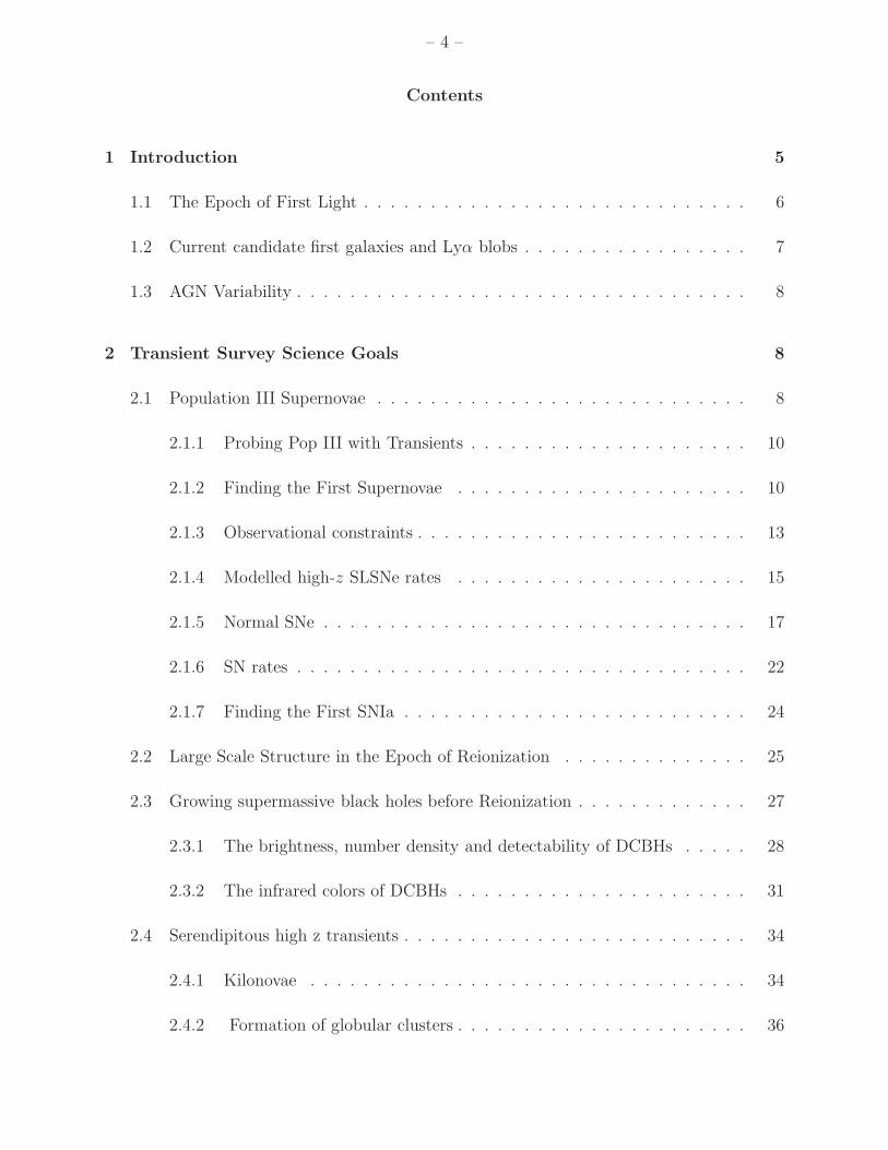
found in a distant galaxy CR7 (Figure 1). These identifications rely heavily on theoretical

models of the radiation from first stars (e.g., Pallottini et al. 2015; Xu et al. 2016; Yajima &

Khochfar 2017) or direct collapse black holes (DCBHs) (e.g., Pacucci et al. 2017; Agarwal

et al. 2016, 2017), which was disputed by Bowler et al. (2017).

The SED of CR7 is shown in Figure 1 (Bowler et al. 2017). A shallow, wide field survey

with JWST is sufficiently deep to discover luminous Lyα emitters like CR7. Matthee et al.

(2015) found that the luminous end of the luminosity function of Lyα emitters at z = 6.6 is

comparable to the luminosity function at z = 3 – 5.7, and is consistent with no evolution

at the bright end since z ∼ 3. The number density of luminous Lyα emitters is thus found

to be much more common than expected. The space density is 1.4+1.2−0.7 × 10−5 Mpc−3.

From Figure 1, we see that such targets can be easily discovered in a survey that goes to

27th mag in 2µm and 4.4µm. They are characterized by very red colors in this wavelength

range. Note, however, Bowler et al. (2017) found a blue [3.6]-[4.5] color based on Spitzer

data, and argued that CR7 is likely a low-mass, narrow-line AGN or is associated with a

young, low-metallicity (∼ 1/200Z⊙) star-burst.

In the design of FLARE, we expect to discover from 20-50 luminous Lyα emitters per

unit redshift bin at z ∼ 6-10 assuming a non-evolving rate of luminous Lyα emitters.

– 8 –

1.3. AGN Variability

Among the high redshift transients FLARE will detect are AGN. These are signposts

to the formation of the Supermassive Black Holes (SMBH) that we know are catapulted

from stellar seeds to >∼ 109M⊙ in the first half billion years of the Universe. Our comoving

volume between redshift 6 and 7 is approximately one million Mpc3. If every galaxy with

a mass exceeding the Milky Way’s has an SMBH, that volume contains 104 SMBH. A

signature of these is Tidal Distortion Events (TDEs), manifesting themselves as order of

magnitude flares in rise times of (1+z) times 30 days. Assuming steady growth between z =

20 and z = 6, each 107 solar mass SMBH is adding 0.01 solar mass per year. If 10% of this

material is stars, the rate of TDEs is of order ten per year. What makes these objects high-z

detectable, as is also true of SLSNe, is that accretion or shocks make them UV bright, more

like flat spectrum sources than the 10000K black bodies that normal photosphere-like SNe

resemble. Caplar et al (2016) find that the amplitude of AGN variation in PTF and SDSS

is typically a tenth of a magnitude, but, interestingly, this goes up by a factor of 5 in the

UV, which is where FLARE will observe at high z.

2. Transient Survey Science Goals

The purpose of the survey is to find transients as witnesses of the state of the Universe

when the first stars and black holes were formed. As we shall see, an appropriate search

strategy is a mosaic approach with only modestly deep individual exposures. In §3 a 0.1

sq deg field is considered to reach into this wide-field regime and place constraints on the

massive Pop III star formation rate density.

2.1. Population III Supernovae

How massive can the first stars, the so-called Population III (Pop III) grow (Bromm

2013)? This question is important in order to determine the nature of the death of

these stars, which in turn governs the feedback exerted by them on their surroundings

– 9 –

Fig. 1.— Left: COSMOS Redshift 7 (abbreviated to CR7)is a bright galaxy found in the

COSMOS field (Matthee et al. 2015; Sobral et al. 2015). Right: The SEDs of the three

components of CR7 are plotted in green (A), purple (B) and red (C), together with the

best-fitting Bruzual & Charlot (2003) model shown as the solid line in each case. The solid

vertical grey lines show the observed wavelengths of the confirmed Lyα and He II emission

lines, whereas the dotted vertical lines show for reference the wavelengths of other rest-frame

UV and optical lines that have been detected or inferred in other high-redshift Lyman Break

Galaxies (Stark et al. 2015a,b; de Barros et al. 2016; Smit et al. 2014; Smidt et al. 2016).

(Maeder & Meynet 2012). To address it, simulations have to be pushed into the radiation

hydrodynamic regime, where protostars more massive than ∼ 10M⊙ emit ionizing photons,

resulting in the build-up of ultra-compact H II regions (Stacy et al. 2012; Hosokawa et

al. 2011, 2015; Hirano et al. 2014). The roughly bi-conical H II regions then begin to

photo-evaporate the proto-stellar disk, thus choking off the gas supply for further accretion

(McKee & Tan 2008). Upper masses thus reached are typically in the vicinity of a few

times 10M⊙, such that the most likely fate encountered by the first stars is a core-collapse

supernova. On the other hand, the prediction is that the primordial initial mass function

(IMF) was rather broad, extending both to lower and (possibly significantly) higher masses.

The latter would imply that BH remnants should be quite common as well. In rarer cases

pair-instability supernova (PISN) progenitors would give rise to hyper-energetic explosions.

See also Woosley et al (2002), Heger et al (2003), Heger & Woosley (2002), Kasen et al

(2011), and references therein.

– 10 –

2.1.1. Probing Pop III with Transients

Transients are the targets of choice because they are the brightest individual objects,

whereas not even the first galaxies are detected in the same observations. Testing Pop III

predictions is challenging, given that Pop III stars are short-lived, and that rapid initial

enrichment hides Pop III star formation from view, such that even the deepest JWST

exposures will typically tend to see metal-enriched, Population II, stellar systems. Therefore,

a more indirect strategy is required. A promising approach is to constrain the extreme

ends of the Pop III IMF. On the high-mass end, the search for PISNe in upcoming JWST

surveys will tell us whether primordial star formation led to masses in excess of ∼ 150M⊙,

the threshold for the onset of the pair-production instability. Individual PISN events are

bright enough to be detected with the JWST, but the challenge will be their low surface

density, such that a wide area needs to be searched (Hummel et al. 2012; Pan et al. 2012;

Whalen et al. 2013).

2.1.2. Finding the First Supernovae

The cosmic dark ages ended with the formation of the first stars at z ∼ 20, or ∼ 200

Myr after the Big Bang (e.g., Bromm et al. 2009; Bromm & Yoshida 2011; Whalen 2013).

The first stars began cosmological reionization (Whalen et al. 2004; Alvarez et al. 2006; Abel

et al. 2007), enriched the primeval universe with the first heavy elements (Mackey et al.

2003; Smith & Sigurdsson 2007; Whalen et al. 2008; Joggerst et al. 2010; Safranek-Shrader

et al. 2014), populated the first galaxies (Johnson et al. 2009; Pawlik et al. 2011; Wise

et al. 2012; O’Shea et al. 2015), and may be the origin of the first supermassive black holes

(Whalen & Fryer 2012; Johnson et al. 2013b; Woods et al. 2017; Smidt et al. 2017). In

spite of their importance to the early universe, not much is known about the properties of

Pop III stars, as not even JWST or 30 - 40 m class telescopes such as the Giant Magellan

Telescope (GMT), the Thirty-Meter Telescope (TMT), or the Extremely Large Telescope

(ELT) will be able to see them (Rydberg et al. 2010). And while the initial conditions for

Pop III star formation are well understood, having been constrained by measurements of

– 11 –

primordial density fluctuations by both WMAP and Planck, numerical simulations cannot

yet determine the masses of primordial stars from first principles (e.g., Bromm et al. 2009;

Bromm & Yoshida 2011; Whalen 2013). However, some of these models suggest that

they may have ranged from a few tens of solar masses to ∼ 1000 M⊙ , with a fairly flat

distribution in mass (Hirano et al. 2014, 2015). See also Woosley (2017)

High-z supernovae (SNe) could directly probe the first generations of stars and their

formation rates because they can be observed at great distances and, to some degree, the

mass of the progenitor can be inferred from the light curve of the explosion (Tanaka et al.

2013; de Souza et al. 2013, 2014). 1D Lagrangian stellar evolution models (Heger & Woosley

2002) predict that 8 - 40 M⊙ nonrotating Pop III stars die as core-collapse (CC) SNe and

that 40 - 90 M⊙ stars collapse to BHs. If the stars are in rapid rotation, they can produce

a GRB (Bromm & Loeb 2006; Mesler et al. 2014) or a hypernova (HN; e.g., Nomoto et al.

2010). 10 - 40 M⊙ stars can also eject shells prior to death, and the subsequent collision of

the SN ejecta with the shell can produce highly luminous events that are brighter than the

explosion itself (pulsational PISNe, or PPI SNe; Woosley et al. 2007; Chen et al. 2014c).

At ∼ 100 M⊙ non-rotating Pop III stars can encounter the pair instability (PI). At

100 - 140 M⊙ the PI causes the ejection of multiple, massive shells instead of the complete

destruction of the star (Woosley et al 2007).Rotation can cause stars to explode as PISNe

at masses as low as ∼ 85 M⊙ (rotational PISNe, or RPI SNe; (Chatzopoulos & Wheeler

2012; Chatzopoulos et al. 2013);Yoon et al (2012). Above 260 M⊙ stars encounter the

photodisintegration with 140 - 260 M⊙ stars exploding as highly energetic thermonuclear

PI SNe (Rakavy & Shaviv 1967; Barkat et al. 1967; Joggerst & Whalen 2011; Chen et al.

2014a). Finally, at much higher masses (>∼ 50,000 M⊙ ) some stars may die as extremely

energetic thermonuclear SNe triggered by the general relativistic instability (Montero et al.

2012; Chen et al. 2014b). Such events could occur in atomically cooled halos at z ∼ 15 -

20, heralding the birth of DCBHs, and thus the first quasars (Johnson et al. 2013a; Whalen

et al. 2013d,c,f).

Superluminous supernovae (SLSNe) can be another critical probe of the deaths of

the first stars, because those events are bright (M < −20.5 mag) (De Cia et al 2017;

– 12 –

Lunnan et al 2017) and have UV-luminous SEDs in the rest-frame. SLSNe are typically

2 – 3 magnitudes brighter than SNe Ia, and 4 or more magnitudes brighter than typical

core-collapse SNe. Observationally, there are two known types of SLSNe. Hydrogen-rich

SLSN II are thought to gain their extremely high luminosity from the collision between

the expanding SN ejecta and a dense circumstellar shell ejected prior to explosion. The

mechanism of the explosion itself is less clear, because it is hidden behind the dense CSM

cloud. Hydrogen-deficient SLSNe, called SLSN I, do not show signs for such a violent

collisional interaction, thus, they are thought to be powered by the spin-down of a magnetar

resulting from the core collapse of an extremely massive progenitor star (Nicholl et al 2017).

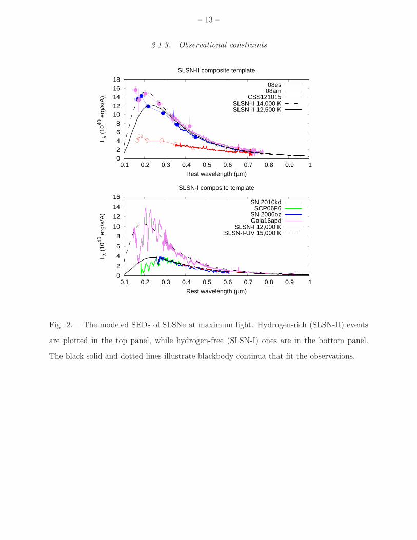
We have modeled the rest-frame SED of SLSNe I and II using the available data of

several well-observed local events (see Figure 2) downloaded from the Weizmann Interactive

Supernova Repository1 and the Open Supernova Catalog2. The UV-optical spectra taken

close to maximum light, after scaling to match photometry, have been corrected for

extinction and distance. Figure 2 shows the final composite spectra together with scaled

blackbodies that fit the continuum. Since SLSN spectra are not homogeneous, we fit two

blackbodies having different temperatures and scale factors (plotted with solid and dashed

lines, respectively) to represent the range of luminosities for both SLSN types.

In Figure 3 we plot the model SEDs of SLSNe redshifted between z = 1 and z = 10.

It is seen that detection with JWST between 2 – 4 micron can be feasible for both types

even at z ∼ 10, provided SLSNe do exist at such high redshift. Fig. 3 suggests that the

detection, in principle, could be pushed above z = 10, but time dilation that increases the

timescale of transients with 1+ z, limits the practical discovery efficiency of the intrinsically

slowly evolving SLSNe at such high redshifts.

1https://wiserep.weizmann.ac.il/

2https://sne.space

– 13 –

2.1.3. Observational constraints

0 2 4 6 8

10 12 14 16 18

0.1 0.2 0.3 0.4 0.5 0.6 0.7 0.8 0.9 1

L λ (

1040

erg

/s/A

)

Rest wavelength (µm)

SLSN-II composite template

08es08am

CSS121015SLSN-II 14,000 KSLSN-II 12,500 K

0

2

4

6

8

10

12

14

16

0.1 0.2 0.3 0.4 0.5 0.6 0.7 0.8 0.9 1

L λ (

1040

erg

/s/A

)

Rest wavelength (µm)

SLSN-I composite template

SN 2010kdSCP06F6

SN 2006ozGaia16apd

SLSN-I 12,000 KSLSN-I-UV 15,000 K

Fig. 2.— The modeled SEDs of SLSNe at maximum light. Hydrogen-rich (SLSN-II) events

are plotted in the top panel, while hydrogen-free (SLSN-I) ones are in the bottom panel.

The black solid and dotted lines illustrate blackbody continua that fit the observations.

– 14 –

0.001

0.01

0.1

1

10

100

0.1 0.2 0.3 0.5 1 2 3 4 5 7 9

20

22

24

26

28

30

z=1.0

z=2.0

z=6.0

z=10

Obs

erve

d flu

x (µ

Jy)

Obs

erve

d A

B-m

agni

tude

Observed wavelength (µm)

SLSN-I

ground limitNIRCAM limit

0.001

0.01

0.1

1

10

100

0.1 0.2 0.3 0.5 1 2 3 4 5 7 9

20

22

24

26

28

30

z=1.0

z=2.0

z=6.0

z=10

Obs

erve

d flu

x (µ

Jy)

Obs

erve

d A

B-m

agni

tude

Observed wavelength (µm)

SLSN-II

ground limitNIRCAM limit

Fig. 3.— The model SEDs of SLSNe (plotted with colored solid and dashed lines) at different

redshifts. Top panel: SLSN-I, lower panel: SLSN-II. The SEDs plotted with dashed lines

correspond to the models having higher temperatures (see Fig.2). Dashed red and black

horizontal lines represent the detection sensitivity limits from the ground and with JWST,

respectively.

The expected rate of SLSNe beyond z > 1 can be estimated from their observed local

rates. Locally, superluminous supernovae (SLSNe) are rare events. Relatively shallow,

flux-limited surveys like CRTS, PTF, and ASASSN discover just a few SLSNe for roughly

– 15 –

every 100 normal luminosity SNe. Obviously these surveys can search for SLSNe in much

larger effective volumes than for normal luminosity SNe, so the rate of SLSNe is but a

fraction of the total SN population’s rate. Quimby et al. (2013) measured a SLSN-like rate

of 199+137−86 events/Gpc3/yr (h3

71) at z = 0.16, which is about 1/1000th of the core-collapse

rate at this redshift. Prajs et al. (2017) measure a rate that is roughly twice as high at

z = 1.13, and Cooke et al. (2012) estimate that the rate is higher by at least another factor

of 5 at 2 < z < 4. Given our current understanding that SLSNe originate with the deaths of

very massive stars typically in low-metallicity environments, such an increase in rate with

redshift is to be expected. The precise redshift evolution is of great value to measure as it

can either be used to reveal how environmental factors affect the production of SLSNe (and

thus help reveal their physical origin), or it can be used to probe how the production of the

most massive stars evolves in relation to lower-mass stars (i.e. the SLSN rate evolution may

help reveal any changes in the stellar IMF with redshift; Tanaka et al. 2013).

2.1.4. Modelled high-z SLSNe rates

Observations show a strong preference for SLSNe toward high star-forming, low-

metallicity environments (Lunnan et al. 2014; Leloudas et al. 2015). As such, SLSNe are

expected to trace the cosmic star formation history. This is evident from the increase in the

observed volumetric rate out to z ∼ 4 (cosmic star formation peaks at z ∼ 2–3, see, e.g.,

Hopkins & Beacom 2006; Moster et al. 2017). The metallicity dependence is likely related

to the SLSN production mechanism and dependent on progenitor properties.

To model the comoving SLSN rate as a function of redshift, we combine a star

formation rate model (ρ∗) with a metallicity-dependent efficiency ǫZ for their formation, i.e.

nSLSNe(z) = ǫZ(z)ρ∗(z). (1)

This method is based on the rate modelling of GRBs by Trenti et al. (2013). We use

DRAGONS’ semi-analytical galaxy-formation model (Mutch et al. 2016), which shows good

agreement with both observations and other models. The efficiency function is the key to

accounting for different SLSN progenitor models via metallicity. As progenitor models are

– 16 –

poorly constrained, we employ the following simple, empirically-motivated prescription.

Using the mean stellar metallicity of every galaxy at each simulated redshift, we calculate a

SLSN production efficiency factor (using stellar evolution simulations by Yoon et al. 2006)

for each galaxy and then average over all galaxies at that redshift. The basic form for the

efficiency factor is higher efficiency for lower metallicities with an adjustable lower threshold

plateau in place at higher metallicities (as SLSNe may still occur in these environments).

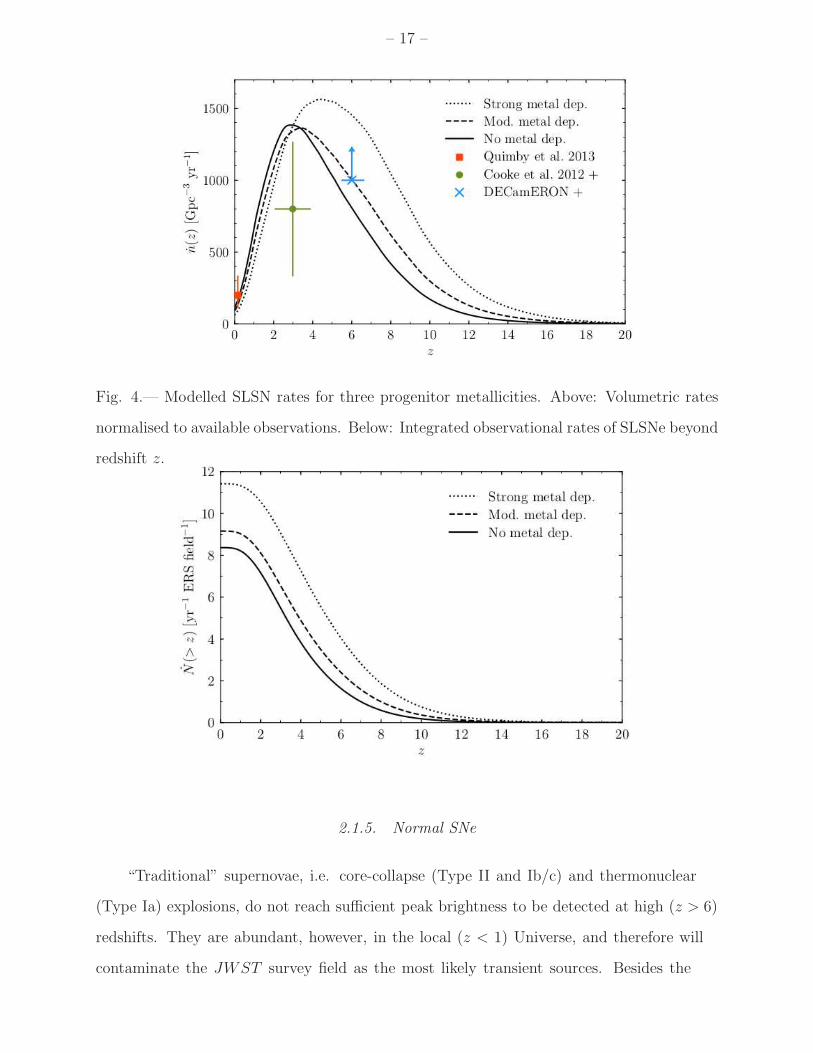
The resulting volumetric rate has been normalised to fit the observed rates of Quimby

et al (2013), Cooke et al (2012), and more recent analysis by Cooke and Curtin (in

preparation). The highest redshift SLSN candidate has been detected by Mould et al (2017)

in deep fields observed with DECam. Their lower limit of 1 deg−2 with AB < –22.5 mag

requires an order of magnitude correction for SLSNe down to –21.5 (Quimby et al 2013).

This is included in the upper panel of Figure 4 and converted into an observational rate

using

NSLSNe(z) =nSLSNe(z)

1 + z

dV

dz. (2)

The lower panel of Figure 4 shows the integrated SLSN rate beyond redshift z for three

models (strong, moderate and no metallicity dependence).

– 17 –

Fig. 4.— Modelled SLSN rates for three progenitor metallicities. Above: Volumetric rates

normalised to available observations. Below: Integrated observational rates of SLSNe beyond

redshift z.

2.1.5. Normal SNe

“Traditional” supernovae, i.e. core-collapse (Type II and Ib/c) and thermonuclear

(Type Ia) explosions, do not reach sufficient peak brightness to be detected at high (z > 6)

redshifts. They are abundant, however, in the local (z < 1) Universe, and therefore will

contaminate the JWST survey field as the most likely transient sources. Besides the

– 18 –

need of filtering out such contaminants from the sample, both CC and Type Ia SNe

could be important in probing the star formation rate (SFR) in the redshift space of

z > 1. To test the detectability of such kind of SNe with JWST , we used the various SN

spectral templates of Nugent (1997) that extend from 0.1µ to 2.5µ in wavelength. At first

the template closest to maximum light was selected, in order to get constraints on the

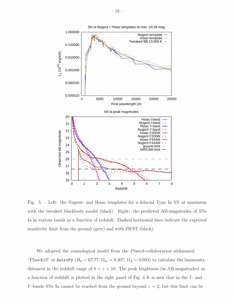
detectability from the maximum distance. Fig. 4 shows the Nugent Ia template compared

to the more recent Hsiao-template (Hsiao et al. 2007) tweaked blackbody that was applied

to model the approximate behavior of the spectral energy distribution (SED) from the UV

to the near-IR. This blackbody fit was applied during the further calculations.

– 19 –

0.000010

0.000100

0.001000

0.010000

0.100000

1.000000

0 5000 10000 15000 20000 25000

L λ (

1040

erg

/s/A

)

Rest wavelength (A)

SN Ia Nugent + Hsiao templates at max -19.26 mag

Nugent templateHsiao template

Tweaked BB 13,000 K

20

21

22

23

24

25

26

27

28

29 0 1 2 3 4 5 6 7 8

Obs

erve

d A

B-m

agni

tude

Redshift

SN Ia peak magnitudes

Hsiao I-bandNugent I-bandHsiao Y-band

Nugent Y-bandHsiao F200W

Nugent F200WHsiao F444W

Nugent F444Wground limit

NIRCAM limit

Fig. 5.— Left: the Nugent- and Hsiao templates for a fiducial Type Ia SN at maximum

with the tweaked blackbody model (black). Right: the predicted AB-magnitudes of SNe

Ia in various bands as a function of redshift. Dashed horizontal lines indicate the expected

sensitivity limit from the ground (grey) and with JWST (black).

We adopted the cosmological model from the P lanck-collaboration nicknamed

“Planck13” in AstroPy (H0 = 67.77, Ωm = 0.307, ΩΛ = 0.693) to calculate the luminosity

distances in the redshift range of 0 < z < 10. The peak brightness (in AB-magnitudes) as

a function of redshift is plotted in the right panel of Fig. 4 It is seen that in the I- and

Y -bands SNe Ia cannot be reached from the ground beyond z ∼ 2, but this limit can be

– 20 –

extended up to z ∼ 5 with JWST at 2 and 4.4 microns.

0.001

0.01

0.1

1

10

100

0.5 1 2 3 4 5 7 9

20

22

24

26

28

30

z=0.1

1.0

2.03.0

4.06.0

10.0

Obs

erve

d flu

x (µ

Jy)

Obs

erve

d A

B-m

agni

tude

Observed wavelength (µm)

ground limitNIRCAM limit

Fig. 6.— The SED of SNe Ia at different redshifts (redshifts are color-coded according to the

legend). The figure shows the expected flux densities in µJy, while the right panel shows the

SEDs expressed in AB-magnitudes. The long-dashed horizontal lines illustrate sensitivity

limits corresponding to 26 and 27 AB-magnitudes.

Fig. 5 illustrates which wavelength region of the SED of redshifted Ia SNe remains

above the detection limits for different redshifts. It is seen that the rest-frame UV/B region

of Ia SNe redshifted to z ∼ 4 –5 are still above the JWST detection limit.

These calculations suggest that if a transient (likely a SN) is detected in all 3 bands

(1µ, 2µ and 4.4µ) at appropriate flux levels then it is likely a SNIa within the 0 < z < 2

redshift range. However, if it is detected at 2µ and 4.4µ but not at 1µ then it may be a

SNIa between 2 < z < 5. Note that detection at 1µ is feasible from the ground, so the

JWST survey should be accompanied by a ground-based survey with a sufficiently large

telescope (Subaru or Keck). Such observations are not difficult to schedule because time

dilation greatly reduces criticality.

Note also that the presence of SNeIa above z > 2 requires the existence of a prompt

channel for their progenitors which has negligible delay time after the formation of the

carbon-oxygen (C/O) white dwarf. Thus, the JWST survey can provide very important

– 21 –

constraints on the existence of such a prompt channel.

16

18

20

22

24

26

28

30 0 1 2 3 4 5

Obs

erve

d A

B-m

agni

tude

Redshift

SN II-P peak magnitudes

Nugent Y-bandNugent F200WNugent F444W

ground limitNIRCAM limit

16

18

20

22

24

26

28

30 0 1 2 3 4 5

Obs

erve

d A

B-m

agni

tude

Redshift

SN Ibc peak magnitudes

Nugent Y-bandNugent F200WNugent F444W

ground limitNIRCAM limit

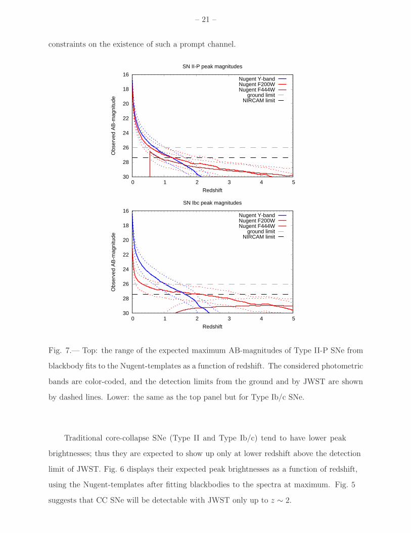
Fig. 7.— Top: the range of the expected maximum AB-magnitudes of Type II-P SNe from

blackbody fits to the Nugent-templates as a function of redshift. The considered photometric

bands are color-coded, and the detection limits from the ground and by JWST are shown

by dashed lines. Lower: the same as the top panel but for Type Ib/c SNe.

Traditional core-collapse SNe (Type II and Type Ib/c) tend to have lower peak

brightnesses; thus they are expected to show up only at lower redshift above the detection

limit of JWST. Fig. 6 displays their expected peak brightnesses as a function of redshift,

using the Nugent-templates after fitting blackbodies to the spectra at maximum. Fig. 5

suggests that CC SNe will be detectable with JWST only up to z ∼ 2.

– 22 –

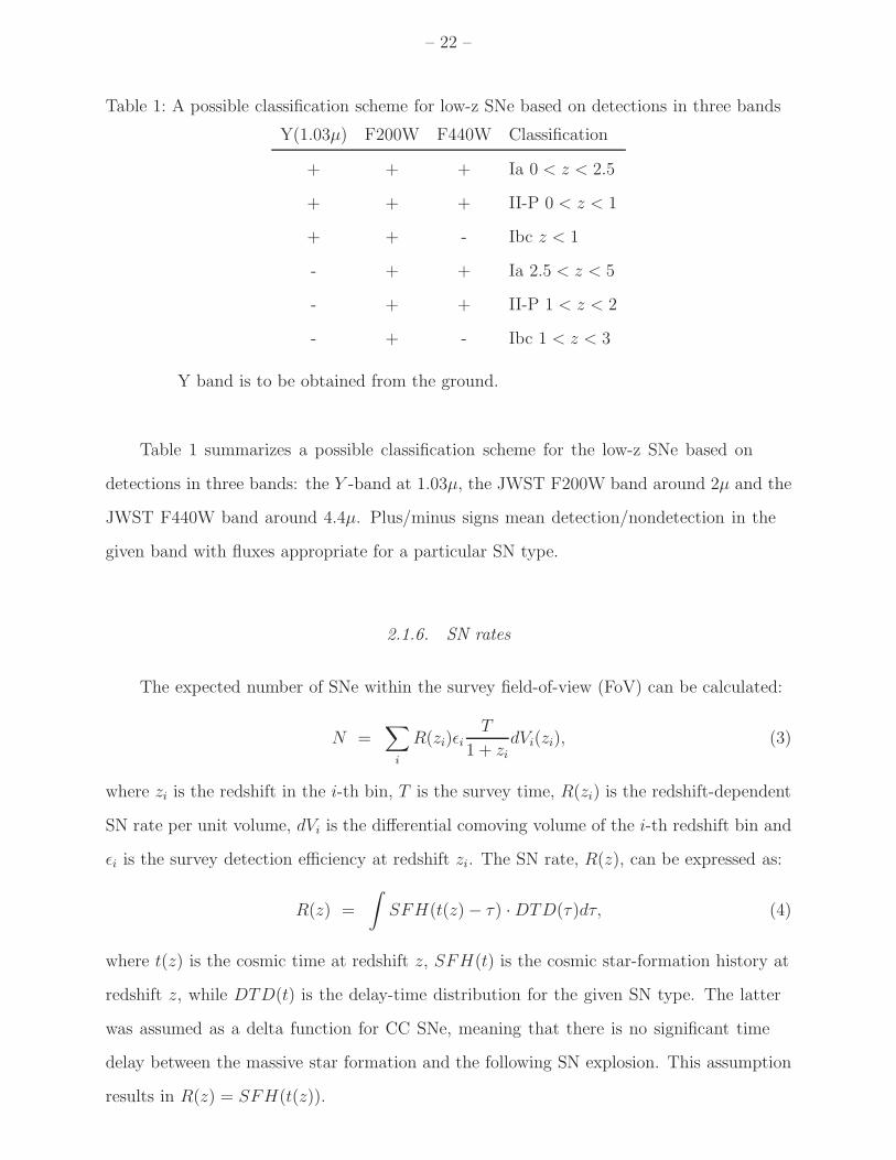
Table 1: A possible classification scheme for low-z SNe based on detections in three bands

Y(1.03µ) F200W F440W Classification

+ + + Ia 0 < z < 2.5

+ + + II-P 0 < z < 1

+ + - Ibc z < 1

- + + Ia 2.5 < z < 5

- + + II-P 1 < z < 2

- + - Ibc 1 < z < 3

Y band is to be obtained from the ground.

Table 1 summarizes a possible classification scheme for the low-z SNe based on

detections in three bands: the Y -band at 1.03µ, the JWST F200W band around 2µ and the

JWST F440W band around 4.4µ. Plus/minus signs mean detection/nondetection in the

given band with fluxes appropriate for a particular SN type.

2.1.6. SN rates

The expected number of SNe within the survey field-of-view (FoV) can be calculated:

N =∑

i

R(zi)ǫi

T

1 + zi

dVi(zi), (3)

where zi is the redshift in the i-th bin, T is the survey time, R(zi) is the redshift-dependent

SN rate per unit volume, dVi is the differential comoving volume of the i-th redshift bin and

ǫi is the survey detection efficiency at redshift zi. The SN rate, R(z), can be expressed as:

R(z) =

∫SFH(t(z) − τ) · DTD(τ)dτ, (4)

where t(z) is the cosmic time at redshift z, SFH(t) is the cosmic star-formation history at

redshift z, while DTD(t) is the delay-time distribution for the given SN type. The latter

was assumed as a delta function for CC SNe, meaning that there is no significant time

delay between the massive star formation and the following SN explosion. This assumption

results in R(z) = SFH(t(z)).

– 23 –

The rate of SNeIa at high (z > 2) redshifts is more uncertain. Current models for

SNIa progenitors, either the single degenerate (SD-) or double degenerate scenario (Iben

& Tutukov 1984), predict a strongly decreasing Ia rate above z ∼ 2. There could be,

however, a prompt Ia population which might explode very shortly after the formation of

the white dwarf (WD). As a first approximation, we assumed that the rate of SNeIa can

be smoothly extended to z > 2 from lower redshifts, following the cosmic star-formation

history function. This approximation gives only a strongly overestimated upper limit for the

expected number of SNeIa at high redshifts. The detected number of such SNe, if any, will

be smaller. We applied the empirical formula by Hopkins & Beacom (2006) to estimate the

SFH(z) function at different redshifts. Values for the absolute SN rates of the particular

SN types were collected from Bazin et al. (2009), while the fractions of Types II and Ibc

within the CC SNe were adopted from Shivvers et al. (2017), being 0.7/0.3. Fig. 6 shows

the adopted SN rates for each type.

Fig. 8.— The assumed rates for each SN type as a function of redshift.

Finally, the number of SNe within the survey FoV was calculated from Eq. 3 for each

type. We adopted T = 100 days for the total survey time and the following detection limits

in the three bands: Y (from ground): 26 AB-mag; F200W (JWST): 27 AB-mag; F440W

(JWST): 27 AB-mag. Assuming 100% survey efficiency (ǫi = 1) as a first approximation,

the results are collected in Table 2.

– 24 –

Table 2: The expected number of SNe of various types in the survey FoV during the survey

time

SN type Mpeak (V) N (Y) N (F200W) N (F440W)

Ia (w/o prompt) −19.3 19 19 13

Ia (w prompt) −19.3 23 45 13

Ibc −17.6 5 6 0

II −16.8 4 16 4

100% detection efficiency assumed.

In total, we can expect ∼ 45 Type Ia, ∼ 16 Type II and ∼ 6 Type Ibc SNe to be

detectable in the survey field. The number for SNeIa is an upper limit, as it contains the

overestimated fraction of the prompt SNeIa. Without the prompt population, the expected

number of SNeIa reduces to 19.

2.1.7. Finding the First SNIa

The survey we propose will be able to discover thermonuclear supernovae to a redshift

approaching z ∼ 4. Although the sparse light curve sampling from our survey may not allow

us to accurately extract the light curve shapes and derive precise cosmological distances to

these SNe, they are nonetheless important in constraining the progenitor systems of SNeIa

and test the evolution of their intrinsic magnitudes. SNeIa at such redshifts will experience

time dilation by a factor of 4–5. Once discovered, they are expected to be visible by JWST

for about 6 months, and bright enough for photometric and spectroscopic followup. They

can be studied by separate programs aiming to directly measure cosmic deceleration at

those redshifts, the ISM towards these SNe, and stellar evolution at very high redshifts.

Because we will also discover ∼50 SNeIa at redshifts around z ∼ 2, our program will serve

as target feeder to programs aiming to measure precision cosmological parameters.

– 25 –

2.2. Large Scale Structure in the Epoch of Reionization

An important question in the epoch of reionization is, can a change in the power

spectrum of the spatial distribution of galaxies be detected between redshift 10 and redshift

6 ? We consider whether this is possible in a 0.1 sq deg FLARE field. A typical distribution

of galaxies in the light cone 6 < z < 10 can be created with TAO, the Theoretical

Astrophysical Observatory (Bernyk et al 2016) and the Millennium simulation (Harker et

al 2006; plus SAGE semianalytics; Croton et al 2016). The brightest galaxies are shown in

Figure 7. The luminosity function is in Figure 8.

– 26 –

Fig. 9.— Brightest galaxies in a light cone made with TAO in a 400 sq arcmin field. Black

points have z = 6; red points z = 7 to blue z = 9; one comoving Mpc is 3 arcmin at z = 6.56.

The higher density of galaxies in the centre left of the field will yield the largest intensity

of ionizing radiation and thus blow a bubble in the neutral hydrogen gas, as seen in the

DRAGONS simulations.

The number of galaxies is made to equal the predictions of the DRAGONS simulation

Mutch et al. (2016).

– 27 –

Fig. 10.— The number of galaxies are bound at each z by the intrinsic UV luminosity function

(upper curve of the shaded envelope) and the dust-corrected UV Luminosity Function (lower

curve of the envelope). Dust is exaggerated at z = 9–10. Integrated in dz = 1 and dM = 1

bins centered on z and M UV (M1600,AB).

2.3. Growing supermassive black holes before Reionization

The first SMBH seeds3 formed when the Universe was younger than ∼500 Myr and

played an important role in the growth of early (z ∼ 7) SMBHs (e.g. Pacucci et al 2015,

Natarajan et al 2017). Much progress has been made in recent years in understanding their

formation, growth and observational signatures, but many questions remain unanswered and

we are yet to detect these sources. Natarajan et al predicted the observational properties

and JWST detectability of black hole seeds, formed by the direct collapse of high-z halos

(e.g. Bromm & Loeb 2003) or as remnants of Pop III stars (e.g. Volunteri & Rees 2005).

When primordial, atomic-cooling halos (Tvir > 104 K) are exposed to a high-intensity

Lyman-Werner flux, Jν > J•

ν (Loeb & Rasio 1994, Lodato & Natarajan 2006, Shang et al

2010) the destruction of H2 molecules allows a rapid, isothermal collapse. The precise value

3Meaning BH beyond stellar mass

– 28 –

of J•

ν depends on several factors, but there is a general consensus that it should fall in the

range 30 < J•

21 < 1000, depending on the spectrum of the sources (Sugimara et al 2014).

Several theoretical works (Bromm 2003, Begelman 2006, Volunteri 2008, Shang et al 2010)

have shown that the result of this collapse is the formation of a Direct Collapse Black Hole

(DCBH) of mass M• ≈ 104−6 M⊙ ( Woods, et al 2017; Umeda et al 2016).

Guided by theoretical estimates in Pacucci et al (2015) and Natarajan et al (2017),

these sources are predicted to be particularly bright in the infrared. In the near infrared,

these sources should be significantly brighter than 28th magnitude (26 on average,

depending on the initial BH mass and on the physical properties of the host halo), while

Pop III seeds are characterized by infrared magnitudes above 29 on average and they could

be unobservable with the JWST . Pacucci et al (2016) (see also Pallottini et al 2015 and

Pacucci et al 2017) claimed the possibility of two z >∼ 6 DCBH candidates in a survey such

as CANDELS/GOODS-S (Illingworth et al 2016) with a significant X-ray emission. DCBHs

are thus high-value targets for the JWST in the infrared. In what follows we present a

general overview on the properties and detectability of DCBHs.

2.3.1. The brightness, number density and detectability of DCBHs

Assuming that a DCBH is accreting at the Eddington rate and that it is Compton-thick

(Yue et al. 2013) (NH>∼ 1024cm−2, where NH is the column number density of the host

galaxy), then its 4.5 µm apparent magnitude is a simple function of black hole mass. The

computation is performed for an object located at z ∼ 13, i.e. well inside the cosmological

period during which the formation of DCBHs is more likely (Yue et al. 2013). A DCBH

seed is predicted to have a mass in the range ∼ 104 − 106 M⊙ (Ferrara et al 2014). When

it grows to >∼ 2 × 106 M⊙, it becomes detectable in the survey that we are proposing

(i.e. brighter than 26.5 mag at 4.5 µm). A DCBH could, however, be characterized by

super-Eddington accretion rates (Pacucci et al 2015). In this case the relation between

mass and brightness is less straightforward to predict, and a DCBH could be detectable

even for masses <∼ 2 × 106 M⊙.

– 29 –

In the literature, the predicted number density of DCBHs widely varies, from ∼ 10−10

to ∼ 10−1 Mpc−3 at z ∼ 10 (comoving units). The large span in the predictions is mainly

due to the uncertainties on the critical external field strength that can fully suppress the H2

formation, the clustering of the potential DCBH formation sites, and the feedback effects.

A summary of the DCBH number densities predicted by different papers is shown in Fig. 11

(taken from Habouzit et al 2016). While the detailed description of each model is found in

the caption of the original paper, here we just want to show the great variety of predictions.

The number density could be even as high as ∼ 0.1 Mpc−3 at z ∼ 13, due to our condition

of producing the observed cosmic near-infrared background fluctuations levels (Yue et al.

2013) from these sources.

Fig. 11.— The number density of DCBHs predicted by several works. The figure is adapted

from Habouzit et al (2016). While the detailed description of each model is found in the

caption of the original paper (and tabulated below), here we only choose to show the great

variety of predictions.

– 30 –

Table 3: symbols & models

symbols nDCBH model M∗

•NH

stars Y13 – 1.2 × 1025 cm−2

filled circles A12, JcLW = 30 106 M⊙ 1025 cm−2

open circles D14, JcLW = 30 106 M⊙ 1025 cm−2

filled squares A12, JcLW = 30 5 × 105 M⊙ 1025 cm−2

open squares D14, JcLW = 30 5 × 105 M⊙ 1025 cm−2

filled triangles A12, JcLW = 30 106 M⊙ 1020 cm−2

open triangles D14, JcLW = 30 106 M⊙ 1020 cm−2

Regarding the detectability, we convert the number density to a surface number

density of DCBHs brighter than some threshold magnitude by specifying a mass function.

Notwithstanding large uncertainties in the DCBH mass function, we can assume a Schechter

formula or a bimodal Gaussian distribution (Ferrara et al 2014). In Fig. 12 we show the

surface number density of DCBHs brighter than 26.5 mag at 4.5 µm, for the DCBH number

density predicted in Agarwal et al (2012) (A12), Yue et al (2013) (Y13) and Dijkstra et

al (2014) (D14) for various DCBH and mass function parameters (see Table 3). Basically,

Compton-thick DCBHs are more detectable because more energy is re-processed to the

rest-frame UV/optical band, then redshifted to the near-infrared band.

– 31 –

Fig. 12.— The surface number density of DCBHs brighter than 26.5 mag at 4.5 µm in

various models. We show the surface number densities predicted in Agarwal et al (2012),

Yue et al (2013) and Dijkstra et al (2014) for various DCBH and mass function parameters.

2.3.2. The infrared colors of DCBHs

According to Pacucci et al (2016), a DCBH has infrared colors significantly different

from the typical QSO or star-forming galaxy. For the photometric filters of our interest,

Y (1 µm), 2.2 and 4.4 µm, we predict photometric colors Y–2.2 and 2.2–4.4 larger than 2.

DCBH candidates can be pre-selected even in purely photometric surveys.

Spectroscopic signatures of DCBHs are: (i) strong He II 1640 A emission line, (ii)

strong Lyα emission (but if the DCBH is extremely Compton-thick, the Lyα emission would

be trapped and converted into continuum emission), (iii) absence of metal lines. Candidates

could also be selected according to their photometric colors (Figure 11) (Pacucci et al 2016).

– 32 –

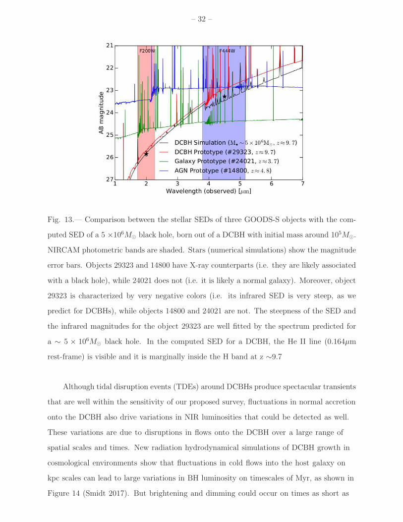
Fig. 13.— Comparison between the stellar SEDs of three GOODS-S objects with the com-

puted SED of a 5 ×106M⊙ black hole, born out of a DCBH with initial mass around 105M⊙.

NIRCAM photometric bands are shaded. Stars (numerical simulations) show the magnitude

error bars. Objects 29323 and 14800 have X-ray counterparts (i.e. they are likely associated

with a black hole), while 24021 does not (i.e. it is likely a normal galaxy). Moreover, object

29323 is characterized by very negative colors (i.e. its infrared SED is very steep, as we

predict for DCBHs), while objects 14800 and 24021 are not. The steepness of the SED and

the infrared magnitudes for the object 29323 are well fitted by the spectrum predicted for

a ∼ 5 × 106M⊙ black hole. In the computed SED for a DCBH, the He II line (0.164µm

rest-frame) is visible and it is marginally inside the H band at z ∼9.7

Although tidal disruption events (TDEs) around DCBHs produce spectacular transients

that are well within the sensitivity of our proposed survey, fluctuations in normal accretion

onto the DCBH also drive variations in NIR luminosities that could be detected as well.

These variations are due to disruptions in flows onto the DCBH over a large range of

spatial scales and times. New radiation hydrodynamical simulations of DCBH growth in

cosmological environments show that fluctuations in cold flows into the host galaxy on

kpc scales can lead to large variations in BH luminosity on timescales of Myr, as shown in

Figure 14 (Smidt 2017). But brightening and dimming could occur on times as short as

– 33 –

the light-crossing time of the BH. Numerical simulations that achieve sub-AU resolution

show that catastrophic baryon collapse in atomically cooled halos leads to the formation of

bursty accretion disks around supermassive primordial protostars, the precursors to DCBHs

(Becerra et al. 2015). Clumpy accretion due to turbulence in the disk can result in changes

in luminosity of about an order of magnitude on timescales of days or weeks in the rest

frame of the nascent DCBH. Such variations should be easily detectable by our proposed

survey.

300 400 500 600 700 800 900Time (Myr)

0.8

0.9

1.0

1.1

1.2

1.3

1.4

Acc

retio

n ra

te /

Edd

ingt

on li

mit

Fig. 14.— DCBH accretion rates as a fraction of the Eddington limit. Blue: no X-ray

feedback. Red: with X-ray feedback from the BH.

According to Kashiyama & Inayoshi (2016) the TDE rate is ∼ 10 per DCBH within

∼ 1 Myr at the DCBH early growth stage. If the TDE only happens at the early stage, and

assuming that the typical lifetime of a DCBH is ∼ 50 Myr, then we expect the TDE rate to

be ∼ 2×10−7 yr−1 per DCBH. Multiplying the surface number density of a steady accreting

DCBH (Fig. 12) by this rate, we obtain the detectability of TDEs: ∼ 10−2 deg−2z−1yr−1 at

maximum at z ∼ 13 in Y13, and ∼ 2 × 10−3 deg−2z−1yr−1 at maximum at z ∼ 7 in A12.

However, if the TDE happens through the whole lifetime of a DCBH, then we expect a rate

as high as ∼ 0.5 deg−2z−1yr−1 in Y13. This value, while obviously lower when compared

to the rate of TDEs for all SMBHs, is a serious consideration for the present survey. A

– 34 –

signature of TDEs is order of magnitude flares in rise times of (1+z) times 30 days.

2.4. Serendipitous high z transients

2.4.1. Kilonovae

The tidal disruption of a neutron star in a binary companion with either another

neutron star or a black hole has long been of astrophysical interest, since it has long been

understood that the decompression of neutron star material could be a site for r-process

nucleosynthesis Lattimer & Schramm 1974; Lattimer et al 1977; Symbalisty & Schramm

1982). Interest was further heightened when it was realized that the same systems could

provide an electromagnetic counterpart for gravitational wave signals Li & Paczynski

1998; Kulkarni 2005; Metzger et al 2010). These systems have been dubbed kilonovae or

macronovae, but we will use the former name. For an excellent review of the entire field,

see Metzger (2017). The expected electromagnetic signatures are illustrated in Fig. 15.

– 35 –

Fig. 15.— The basic picture of the various electromagnetic signatures produced in a merging

neutron star event. The kilonova emission comes from the semi symmetric ejecta. (From ?).

Population synthesis models predict gravity wave detection rates of NS-NS/BH-NS

mergers of ∼ 0.2 − 300 per year, for the full design sensitivities of Advanced LIGO/Virgo

(Abadie et al 2010; Dominik et al 2015). Empirical estimates predict ∼ 8 NS-NS mergers

per year in the Galaxy (Kalogera et al 2004a,b; Kim et al 2015). Numerical models of the

event rate estimate ∼ 1000 Gpc−3 yr−1 (Tanaka 2016) with a spectrum shown in Fig. 16.

– 36 –

Fig. 16.— The spectrum of the relativistic ejecta of a NS-NS merger compared with that of

supernovae (Tanaka 2016).

Models of the disk-wind structure have been performed by Kasen et al (2015) and

the dynamics and nucleosynthesis of BH-NS mergers have been studied by Fernandez et al

(2016) and Metzger (2017) and references therein.

We have begun preliminary modeling with the generalized stellar atmospheres code

PHOENIX (P. Vallely & E. Baron, in preparation). We include some r-process elements in

full NLTE, and the time is right to begin NLTE modeling as the atomic data to construct

the model atoms for all r-process elements is now available (Fontes et al 2017).

Several kilonovae should be visible in our proposed program and understanding these

events is important for understanding the site of the r-process as well as crucial to providing

eletromagnetic counterparts to gravitational wave events.

2.4.2. Formation of globular clusters

Renzini (2017) suggests that a proto globular cluster in the Epoch of Reionization

(EoR) reaches AB = 28 for a Myr . At low metallicity these objects are candidates to

produce SLSNe with 25 < AB < 28. If 5% of the cosmic SFR from z = 9 to 6 were in

globular clusters (GC), we would have 2 x 105 M⊙ /Mpc3 . For M/L = 10−2 that is 2 x 107

– 37 –

L⊙ /Mpc3 . In 1 sq deg dn/dt = ∼1 GC SLSN per year.

Globular clusters are laboratories for SNe as for IMF ∼ m−2 some half of the mass

terminates in SNe. The kinetic energy of a GC of 106M ⊙ is 106× 1012× 1033 = 1 foe.

Depositing 1 foe in it from a SLSN will come close to unbinding the cluster. According

to chemical evolution theory removing the gas from the cluster is required to retain the

observed low metallicity, and a SLSN may well be the agent4.

3. The FLARE JWST Transient Field

Now we need to detail the methodology for an efficient First Transients survey. We

propose to survey the North Ecliptic Pole (NEP) in two colors down to 27.4 mag (AB). This

is very much deeper than the JWST Time-Domain Community Field. The NIRCAM with

filters F200W and F444W is most appropriate to the project. We will also employ NIRISS

for deeper coverage in the F444W band for a small fraction of the field in the parallel

mode. For an Early Release Science time-domain survey, two visits of the NEP field would

be made at two epochs separated by 91.3 days. For these purposes the primary survey

instrument is NIRCAM, with NIRISS in parallel mode. The survey employs two filters,

F200W and F444W with NIRCAM and F444 only with NIRISS. Medium background level

is appropriate. The detector is to be set up to read out the full array, and the readout

pattern is SHALLOW4; the observations employ 3 Groups, 2 Integrations, and 1 Exposures,

in accordance with STScI Exposure Time Calculator tools. This gives a total exposure time

of 322.1s for each pointing and a S/N ratio of 3.1 and 3.2 in F200W and F444W, for targets

of 27.4 mag (AB) and 27. 5 mag (AB), and a S/N ratio of 5.0 in F200W and F444W, for

targets of 26.9 mag (AB) and 27.0 mag (AB), respectively. For efficient telescope steering,

we foresee observations grouped into a 9×5 rectangular mosaic. Full dithering is important

in rejecting spurious signals but carries a prohibitively expensive overhead for a wide

field survey. However, in our simulations of JWST observations, we found that sub-pixel

dithering with 2-POINT-MEDIUM-WITHNIRISS is sufficient for rejecting spurious signals

4See also Recchi et al (2017)

– 38 –

due to hot pixels and cosmic rays. For a fully successful program, one should expect to

revisit the same field multiple times, which will help build up more robust templates and

aid in rejecting cosmic rays.

3.1. Why cluster lensing does not help find more transients

As pointed out in Sullivan et al. (2000) there are three important effects one has

to consider in understanding any gain (or loss) in the supernova detection rate via a

lensing cluster. These are: the area-weighted lensing magnification, the supernova rate as

a function of redshift and the limiting magnitude of the survey. As can be seen in their

Figure 3 and Table 1 for a simulated HST survey, modest gains can be had for 1.5 < z < 2.0

due to the fact that the intrinsic rates are flat or slowly declining at these redshifts and

amplification brings SNe at the lower end of the luminosity function into the realm of

detection. Interestingly, the supernova detection efficiency drops for z < 1.5 as the area

surveyed behind a cluster shrinks in proportion to the amplification factor. Since HST can

easily discover SNe without magnification below these redshifts, by reducing the survey

area one suffers a net loss.

This fact is exacerbated in any survey by JWST to depths of AB = 27. Since the

supernova rate starts dropping dramatically beyond a redshift of 2–3 (driven by the 1 + z

time dilation, see Figure 2 of Sullivan et al. (2000)) and JWST is already sensitive to even

the lowest end of the luminosity function for SNe Ia at these redshifts (and more than 70%

of the core-collapse supernovae), a lensing cluster search provides no net benefit. In fact,

there would be appreciable loss due to the drop in effective area.

3.2. Probabilistic Target Classification

With our choice of filters, we are able to make a preliminary screening by the variability

of the sources and their location on the color-magnitude diagram. Fig. 17 shows as an

example how different objects may be classified. It is clear from the figure that DCBH

stand out clearly as extremely red objects, whereas SLSNe and SNeIa fall on distinct areas

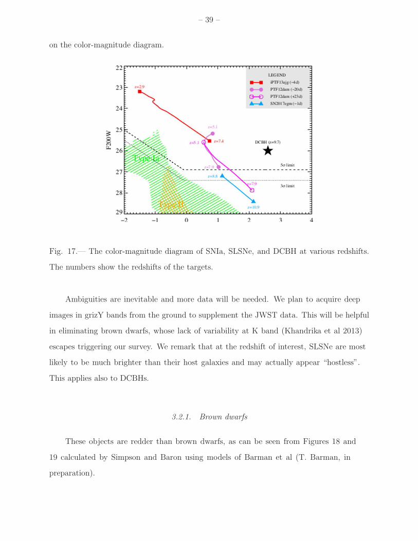
– 39 –

on the color-magnitude diagram.

Fig. 17.— The color-magnitude diagram of SNIa, SLSNe, and DCBH at various redshifts.

The numbers show the redshifts of the targets.

Ambiguities are inevitable and more data will be needed. We plan to acquire deep

images in grizY bands from the ground to supplement the JWST data. This will be helpful

in eliminating brown dwarfs, whose lack of variability at K band (Khandrika et al 2013)

escapes triggering our survey. We remark that at the redshift of interest, SLSNe are most

likely to be much brighter than their host galaxies and may actually appear “hostless”.

This applies also to DCBHs.

3.2.1. Brown dwarfs

These objects are redder than brown dwarfs, as can be seen from Figures 18 and

19 calculated by Simpson and Baron using models of Barman et al (T. Barman, in

preparation).

– 40 –

Fig. 18.— Colors of brown dwarfs of types M, L, T, Y.

Fig. 19.— Colors of brown dwarfs with dusty atmospheres

4. Facilitating First Transients discovery

The vision of the JWST is to discover the first stars to appear in the Universe. For

this to be accomplished in fact with this facility we must see not their faint birth but their

bright SNe. The FLARE project would lay the foundation to do this over the life of the

JWST mission by creating a James Webb Transient Factory (JWTF), in which all the

– 41 –

mission’s repeat imaging data would be analysed for transients.

4.1. The design of the FLARE project

4.1.1. Observations and deliverables with JWST

Our observing plan is tailored to deliver some transients from the epoch of reionization

over the first six months, both single supernovae and transients resulting from the formation

by redshift 6 of SMBHs. But according to §2 the highest redshift supernovae are rare

enough that only operation of a JWTF for five years will find them.

Appropriate deliverables will therefore include the software for a JWTF, developed

at the Weizmann and the Mitchell Institutes, which could be operated at Space Telescope

Science Institute, and also, through a collaboration with Swinburne University and drawing

on the Millennium Simulation and other similar databases, a module of the Theoretical

Astrophysical Observatory which will allow full simulation of all GO proposals for imaging

with JWST by the proposers themselves in the course of preparing Cycle 2 and later cycles.

The Theoretical Astrophysical Observatory (TAO, https://tao.asvo.org.au) houses

data from popular cosmological N-body simulations and galaxy formation models, primarily

focused on survey science. Mock catalogues can be built from the database without the

need for any coding. Results can be funneled through higher-level modules to generate

SEDs, build custom light-cones and images.

TAO will be expanded to include more detailed modelling of the galaxies and SNe at

high redshift relevant to the JWST , and new tools to produce mock observations that

mimic those that JWTF will process. This will allow predictions to be made using the

advanced simulations that TAO hosts and interpretation of the results as they arrive.

– 42 –

4.1.2. Supporting observations and followup strategies

To realise its full potential, time domain astronomy makes serious demands on cadence,

followup, and multiwavelength coverage. High z investigations are less demanding than

local ones due to time dilation, and we anticipate that NEP revisits can be proposed with

normal STScI planned annual cycles. Spectroscopic followup of targets of opportunity

with NIRSpec and ELT instruments may also be a modest imposition on these facilities.

Deep ground based reference fields at shorter wavelengths, however, should be initiated

immediately for the purpose of eliminating foreground objects. The Subaru Stategic

Program (Aihara et al 2017) is a model for such data and adding the NEP to the current

set of fields seems to us to be a priority. X-ray followup of JWST high z transients will also

be vital.

5. Conclusion

The definitive image of the unmistakable structure of the early universe is the WMAP

and P lanck iconic picture (Bennett et al 2003; Ade et al 2016). The vision of JWST is to

link this structure and the associated precision cosmology to the first stars formed from the

pristine gas out there in protogalactic clumps. Those first stars are individually too faint,

and even first galaxies will still be challenging for JWST , especially if a representative

sample be studied.

In this white paper, we have demonstrated that instead of hammering at still images,

observations of transients offer an elegant alternative method of characterizing the early

universe. Information about stellar populations and the IMF is encapsulated in SLSNe,

and TDEs (and the intrinsic variability of the accretion flow) can trace the mysterious

build-up of billion solar mass SMBHs within few hundreds of millions of years. Detecting

and characterizing first SLSNe and TDEs in sufficient numbers are the goals of the FLARE

project for JWST .

We have shown that monitoring with JWST a 0.1 square degree field at 2 and 4

microns and moderate depth can achieve these goals. Ground based deep imaging at shorter

– 43 –

wavelengths will complete the inventory of the field and help avoid false alarms.

After this quantitative confirmation at the level of transient categories, we will move on

to numerical simulations to determine similarly quantitatively how many events need to be

found and which combinations of time baseline, cadence, colour information, and field size

yield the highest success rates in the classification of high-z transients. This will deliver a

solid justification of the significant investment of telescope time over the life of the mission.

We intend to make immediately public all transients found by the FLARE project. This

will enable the community to define and execute follow-up observations of the transients

themselves as well as of their environments of which the high-z transients represent the tips

of their luminosity functions in transparent regions of the early universe. The (1+z)-fold

time dilation makes the planning of such efforts well feasible. We will develop and offer tools

to perform analogous searches for transients in all other JWST fields which throughout the

lifetime of JWST require repeated observations. This will lead to an enlarged homogeneous

real-time database of high-z transients at no extra cost.

– 44 –

REFERENCES

Abel, T., Wise, J. H., & Bryan, G. L. 2007, ApJ, 659, L87

Agarwal, B., Johnson, J. L., Khochfar, S., et al. 2017, MNRAS, 469, 231

Agarwal, B., Johnson, J. L., Zackrisson, E., et al. 2016, MNRAS, 460, 4003

Alvarez, M. A., Bromm, V., & Shapiro, P. R. 2006, ApJ, 639, 621

Barkat, Z., Rakavy, G., & Sack, N. 1967, Physical Review Letters, 18, 379

Becerra, F., Greif, T. H., Springel, V., & Hernquist, L. E. 2015, MNRAS, 446, 2380

Bowler, R. A. A., McLure, R. J., Dunlop, J. S., et al. 2017, MNRAS, 469, 448

Bromm, V., & Loeb, A. 2006, ApJ, 642, 382

Bromm, V., & Yoshida, N. 2011, ARA&A, 49, 373

Bromm, V., Yoshida, N., Hernquist, L., & McKee, C. F. 2009, Nature, 459, 49

Bruzual, G., & Charlot, S. 2003, MNRAS, 344, 1000

Chatzopoulos, E., & Wheeler, J. C. 2012, ApJ, 748, 42

Chatzopoulos, E., Wheeler, J. C., & Couch, S. M. 2013, ApJ, 776, 129

Chen, K.-J., Heger, A., Woosley, S., Almgren, A., & Whalen, D. J. 2014a, ApJ, 792, 44

Chen, K.-J., Heger, A., Woosley, S., et al. 2014b, ApJ, 790, 162

Chen, K.-J., Woosley, S., Heger, A., Almgren, A., & Whalen, D. J. 2014c, ApJ, 792, 28

de Barros, S., Vanzella, E., Amorın, R., et al. 2016, A&A, 585, A51

de Souza, R. S., Ishida, E. E. O., Johnson, J. L., Whalen, D. J., & Mesinger, A. 2013,

MNRAS, 436, 1555

de Souza, R. S., Ishida, E. E. O., Whalen, D. J., Johnson, J. L., & Ferrara, A. 2014,

MNRAS, 442, 1640

– 45 –

Heger, A., & Woosley, S. E. 2002, ApJ, 567, 532

Hirano, S., Hosokawa, T., Yoshida, N., Omukai, K., & Yorke, H. W. 2015, MNRAS, 448,

568

Hirano, S., Hosokawa, T., Yoshida, N., et al. 2014, ApJ, 781, 60

Hopkins, A. M., & Beacom, J. F. 2006, ApJ, 651, 142

Hummel, J. A., Pawlik, A. H., Milosavljevic, M., & Bromm, V. 2012, ApJ, 755, 72

Joggerst, C. C., Almgren, A., Bell, J., et al. 2010, ApJ, 709, 11

Joggerst, C. C., & Whalen, D. J. 2011, ApJ, 728, 129

Johnson, J. L., Greif, T. H., Bromm, V., Klessen, R. S., & Ippolito, J. 2009, MNRAS, 399,

37

Johnson, J. L., Whalen, D. J., Even, W., et al. 2013a, ApJ, 775, 107

Johnson, J. L., Whalen, D. J., Li, H., & Holz, D. E. 2013b, ApJ, 771, 116

Leloudas, G., Schulze, S., Kruhler, T., et al. 2015, MNRAS, 449, 917

Lunnan, R., Chornock, R., Berger, E., et al. 2014, ApJ, 787, 138

Mackey, J., Bromm, V., & Hernquist, L. 2003, ApJ, 586, 1

Magg, M., Hartwig, T., Glover, S. C. O., Klessen, R. S., & Whalen, D. J. 2016, MNRAS,

462, 3591

Matthee, J., Sobral, D., Santos, S., et al. 2015, MNRAS, 451, 400

Mesler, R. A., Whalen, D. J., Smidt, J., et al. 2014, ApJ, 787, 91

Montero, P. J., Janka, H.-T., & Muller, E. 2012, ApJ, 749, 37

Moster, B. P., Naab, T., & White, S. D. M. 2017, ArXiv e-prints, arXiv:1705.05373

Mutch, S. J., Geil, P. M., Poole, G. B., et al. 2016, MNRAS, 462, 250

– 46 –

Nomoto, K., Tanaka, M., Tominaga, N., & Maeda, K. 2010, New Astronomy Reviews, 54,

191

O’Shea, B. W., Wise, J. H., Xu, H., & Norman, M. L. 2015, ApJ, 807, L12

Ouchi, M., Shimasaku, K., Furusawa, H., et al. 2010, ApJ, 723, 869

Pacucci, F., Pallottini, A., Ferrara, A., & Gallerani, S. 2017, MNRAS, 468, L77

Pallottini, A., Ferrara, A., Pacucci, F., et al. 2015, MNRAS, 453, 2465

Pan, T., Kasen, D., & Loeb, A. 2012, MNRAS, 422, 2701

Pawlik, A. H., Milosavljevic, M., & Bromm, V. 2011, ApJ, 731, 54

Postman, M., Coe, D., Benıtez, N., et al. 2012, ApJS, 199, 25

Rakavy, G., & Shaviv, G. 1967, ApJ, 148, 803

Robertson, B. E., & Ellis, R. S. 2012, ApJ, 744, 95

Rydberg, C. E., Zackrisson, E., & Scott, P. 2010, in Cosmic Radiation Fields: Sources in

the early Universe (CRF 2010), ed. M. Raue, T. Kneiske, D. Horns, D. Elsaesser, &

P. Hauschildt , 26

Safranek-Shrader, C., Milosavljevic, M., & Bromm, V. 2014, MNRAS, 438, 1669

Smidt, J., Whalen, D. J., Chatzopoulos, E., et al. 2015, ApJ, 805, 44

Smidt, J., Whalen, D. J., Johnson, J. L., & Li, H. 2017, arXiv:1703.00449, arXiv:1703.00449

Smidt, J., Whalen, D. J., Wiggins, B. K., et al. 2014, ApJ, 797, 97

Smidt, J., Wiggins, B. K., & Johnson, J. L. 2016, ApJ, 829, L6

Smit, R., Bouwens, R. J., Labbe, I., et al. 2014, ApJ, 784, 58

Smith, B. D., & Sigurdsson, S. 2007, ApJ, 661, L5

Sobral, D., Matthee, J., Darvish, B., et al. 2015, ApJ, 808, 139

– 47 –

Stark, D. P., Richard, J., Charlot, S., et al. 2015a, MNRAS, 450, 1846

Stark, D. P., Walth, G., Charlot, S., et al. 2015b, MNRAS, 454, 1393

Tanaka, M., Moriya, T. J., & Yoshida, N. 2013, MNRAS, 435, 2483

Whalen, D., Abel, T., & Norman, M. L. 2004, ApJ, 610, 14

Whalen, D., van Veelen, B., O’Shea, B. W., & Norman, M. L. 2008, ApJ, 682, 49

Whalen, D. J. 2013, Acta Polytechnica, 53, 573

Whalen, D. J., & Fryer, C. L. 2012, ApJ, 756, L19

Whalen, D. J., Fryer, C. L., Holz, D. E., et al. 2013a, ApJ, 762, L6

Whalen, D. J., Joggerst, C. C., Fryer, C. L., et al. 2013b, ApJ, 768, 95

Whalen, D. J., Johnson, J. L., Smidt, J., et al. 2013c, ApJ, 777, 99

—. 2013d, ApJ, 774, 64

Whalen, D. J., Smidt, J., Even, W., et al. 2014, ApJ, 781, 106

Whalen, D. J., Smidt, J., Johnson, J. L., et al. 2013e, arXiv:1312.6330, arXiv:1312.6330

Whalen, D. J., Even, W., Smidt, J., et al. 2013f, ApJ, 778, 17

Whalen, D. J., Even, W., Frey, L. H., et al. 2013g, ApJ, 777, 110

Whalen, D. J., Even, W., Lovekin, C. C., et al. 2013h, ApJ, 768, 195

Wise, J. H., Turk, M. J., Norman, M. L., & Abel, T. 2012, ApJ, 745, 50

Woods, T. E., Heger, A., Whalen, D. J., Haemmerle, L., & Klessen, R. S. 2017,

arXiv:1703.07480, arXiv:1703.07480

Woosley, S. E., Blinnikov, S., & Heger, A. 2007, Nature, 450, 390

Xu, H., Norman, M. L., O’Shea, B. W., & Wise, J. H. 2016, ApJ, 823, 140

Yajima, H., & Khochfar, S. 2017, MNRAS, 467, L51

– 48 –

Yue, B., Ferrara, A., Salvaterra, R., Xu, Y., & Chen, X. 2013, MNRAS, 433, 1556

Supplementary

Abadie, J., et al. 2010, Classical and Quantum Gravity, 27, 173001

Ade, P. et al 2016, A&A, 594, 17

Aihara, H. et al 2017, arxiv 1704.5858

Bazin, G. et al. 2009, A&A, 499, 653

Bennett, C. L. et al 2003, ApJS, 148, 97

Bernyk, M. et al 2016, ApJS, 223, 9

Bromm, V. 2013, Rep Prog Phys, 76, 2901

Caplar, N. et al 2016, arxiv 1611.3082

Cooke, J. et al. 2012, Nature, 491, 228

Croton, D. et al 2016, ApJS, 222, 22

Dijkstra, M. et al (2014, MNRAS, 442, 2036

Dominik, M., Berti, E., O’Shaughnessy, R., Mandel, I., Belczynski, K., Fryer, C., Holz,

D. E., Bulik, T., & Pannarale, F. 2015, ApJ, 806, 263

Fernandez, R., Foucart, F., Kasen, D., Lippuner, J., Desai, D., & Roberts, L. F. 2016,

ArXiv e-prints, 1612.04829

Ferrara, A. et al 2014, MNRAS, 443, 2410

Fontes, C. J., Fryer, C. L., Hungerford, A. L., Wollaeger, R. T., Rosswog, S., & Berger,

E. 2017, ArXiv e-prints, 1702.02990

Furnaletto, S. et al. 2006, PhysR, 433, 181

Habouzit, M. et al 2016, MNRAS, 463, 529

This manuscript was prepared with the AAS LATEX macros v5.2.

– 49 –

Harker, G. et al 2006, MNRAS, 367, 1039

Heger, A.; Fryer, C. L.; Woosley, S. E.; Langer, N.; Hartmann, D. 2003, ApJ, 591, 288

Hosokawa, T. et al. 2011, Sci, 344, 1250

Hosokawa, T. et al. 2016, ApJ, 824, 119

Hsiao, E. et al. 2007, ApJ, 663, 1187

Iben, I. & Tutukov, A. 1984, ApJ, 284, 719

Kasen, Daniel; Woosley, S. E.; Heger, Alexander 2011, ApJ, 734, 102

Kalogera, V., Kim, C., Lorimer, D. R., Burgay, M., D’Amico, N., Possenti, A.,

Manchester, R. N., Lyne, A. G., Joshi, B. C., McLaughlin, M. A., Kramer, M., Sarkissian,

J. M., & Camilo, F. 2004a, ApJ, 614, L137

—. 2004b, ApJ, 601, L179

Kasen, D., Fernandez, R., & Metzger, B. D. 2015, MNRAS, 450, 1777

Kashiyama, K. & Inayoshi, K. 2016, ApJ, 826, 80

Khandrika, H. et al 2013, AJ, 145, 71

Kim, C., Perera, B. B. P., & McLaughlin, M. A. 2015, MNRAS, 448, 928

Kulkarni, S. R. 2005, ArXiv Astrophysics e-prints, astro-ph/0510256

Lattimer, J. M., Mackie, F., Ravenhall, D. G., & Schramm, D. N. 1977, ApJ, 213, 225

Lattimer, J. M. & Schramm, D. N. 1974, ApJ, 192, L145

Li, L.-X. & Paczynski, B. 1998, ApJ, 507, L59

Loeb, A. & Furlanetto, S. 2013, The First Galaxies in the Universe, Princeton

University Press

McKee, C. & Tan, J. 2008, ApJ, 681, 771

Maeder, A. & Meynet, G. 2012, Rev Mod Phys, 84, 25

– 50 –

Metzger, B. D. 2017, Living Reviews in Relativity, 20, 3

Metzger, B. D. & Berger, E. 2012, ApJ, 746, 48

Metzger, B. D., Martınez-Pinedo, G., Darbha, S., Quataert, E., Arcones, A., Kasen,

D., Thomas, R., Nugent, P., Panov, I. V., & Zinner, N. T. 2010, MNRAS, 406, 2650

Mould, J. R., et al 2017, Sci Bull 62(10), 675, arXiv:1704.05967

Natarajan, P., Pacucci, F., Ferrara, A., et al. 2017, ApJ, 838, 117

Nicholl, M. et al 2017, ApJ, 843, 84

Nugent, P. 1997, ApJ, 485, 812

Pacucci, F., Ferrara, A., Volonteri, M., & Dubus, G. 2015, MNRAS, 454, 3771

Pacucci, F. et al. 2016, MNRAS, 459, 1432

Prajs, S. et al 2017, MNRAS, 464, 3568

Quimby, R. et al. 2013, MNRAS 431, 912)

Recchi, S. et al 2017, ApSS, (in press)

Renzini, A., 2017, MNRAS, 469, L63

Shivvers, I. et al. 2017, MNRAS, 471, 4381

Stacy, A. et al. 2012; MNRAS, 422, 290

Sullivan, M. et al. 2000, MNRAS, 312, 442

Symbalisty, E. & Schramm, D. N. 1982, Astrophys. Lett., 22, 143

Tanaka, M. 2016, Advances in Astronomy, 2016, 634197

Trenti, M., Perna, R. & Tacchella, S., 2013, ApJ, 773, L22

Umeda, Hideyuki; Hosokawa, Takashi; Omukai, Kazuyuki; Yoshida, Naoki, 2016,

ApJL, 830, L34

Woosley, S. E.; Heger, A.; Weaver, T. , 2002, RvMP, 74, 1015

– 51 –

Woosley, S. E. 2017, ApJ, 836, 244

Yoon, S.-C., Langer, N. & Norman, C., 2006, A&A, 460, 199

Yoon, S.-C., Dierks, A., & Langer, N. 2012, A&A, 542, A113

Appendix: Pop III SNe

An extensive campaign of radiation hydrodynamical simulations has shown that PI

SNe, PPI SNe and Type IIn SNe will be visible to JWST and the extremely large telescopes

(ELTs) at z >∼ 20 (Whalen et al. 2013a,g,h, 2014). CC SNe will be visible to these telescopes

at z = 10 – 20 (Whalen et al. 2013b) and rotating PISNe and hypernovae will be visible

out to z ∼ 10 (Smidt et al. 2014, 2015). Near infrared (NIR) light curves for 150 – 250

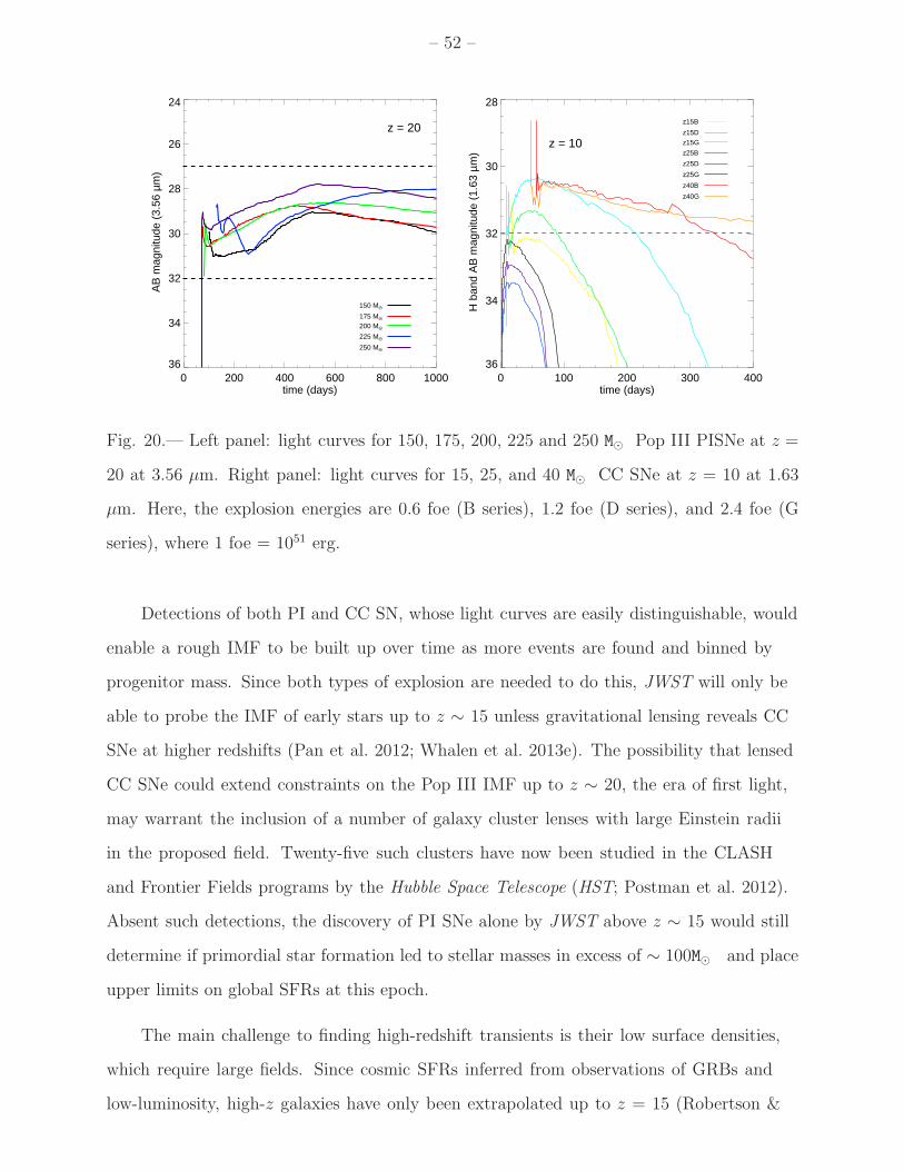
M⊙ PISNe and 15 - 40 M⊙ CC SNe are in Figure 20. These studies demonstrate that the

optimum wavelengths for observing SNe at z = 10 – 20 are 2 – 5 µm. JWST is uniquely

qualified to detect these events because its 40 K temperatures and low thermal noise vastly

simplify its systematics in comparison to ground-based ELT’s, which must contend with

much greater instrument noise and atmospheric transmission in the NIR.

– 52 –

0 200 400 600 800 1000time (days)

36

34

32

30

28

26

24

AB

mag

nitu

de (

3.56

µm

)

150 MO •

175 MO •

200 MO •

225 MO •

250 MO •

z = 20

0 100 200 300 400time (days)

36

34

32

30

28

H b

and

AB

mag

nitu

de (

1.63

µm

)

z15B

z15Dz15G

z25B

z25D

z25G

z40B

z40G

z = 10

Fig. 20.— Left panel: light curves for 150, 175, 200, 225 and 250 M⊙ Pop III PISNe at z =

20 at 3.56 µm. Right panel: light curves for 15, 25, and 40 M⊙ CC SNe at z = 10 at 1.63

µm. Here, the explosion energies are 0.6 foe (B series), 1.2 foe (D series), and 2.4 foe (G

series), where 1 foe = 1051 erg.

Detections of both PI and CC SN, whose light curves are easily distinguishable, would

enable a rough IMF to be built up over time as more events are found and binned by

progenitor mass. Since both types of explosion are needed to do this, JWST will only be

able to probe the IMF of early stars up to z ∼ 15 unless gravitational lensing reveals CC

SNe at higher redshifts (Pan et al. 2012; Whalen et al. 2013e). The possibility that lensed

CC SNe could extend constraints on the Pop III IMF up to z ∼ 20, the era of first light,

may warrant the inclusion of a number of galaxy cluster lenses with large Einstein radii

in the proposed field. Twenty-five such clusters have now been studied in the CLASH

and Frontier Fields programs by the Hubble Space Telescope (HST; Postman et al. 2012).

Absent such detections, the discovery of PI SNe alone by JWST above z ∼ 15 would still

determine if primordial star formation led to stellar masses in excess of ∼ 100M⊙ and place

upper limits on global SFRs at this epoch.

The main challenge to finding high-redshift transients is their low surface densities,

which require large fields. Since cosmic SFRs inferred from observations of GRBs and

low-luminosity, high-z galaxies have only been extrapolated up to z = 15 (Robertson &

– 53 –

Ellis 2012), one must resort to numerical simulations for estimates of SFRs at earlier

times. As shown in the left panel of Figure 21, these rates vary by a factor of 300 at the

highest redshifts, highlighting the present uncertainties in them. However, even at z ∼ 20

- 25 JWST is predicted to find a number of PI SNe (right panel of Figure 21; Hummel

et al. 2012). The optimal search strategy is a mosaic approach with only modestly deep

individual exposures. Our proposed field is well suited to push into this wide-field regime

to place constraints on the SFR density of massive Pop III stars.

However, even the unlikely failure of JWST to harvest any transients in our ERS field

at z >∼ 15 would place useful, strong upper limits on global SFRs in the primordial universe

and could even shed light on the properties of dark matter. Models of early structure

formation with warm dark matter (WDM) predict a suppression of power on small scales

that delays Pop III star formation to z ∼ 15, so the failure to detect SNe at earlier times

might be a signature of such suppression (Magg et al. 2016). Furthermore, any detections

of SNe at z ∼ 10 − 20 would still trace the rise of stellar populations in the first galaxies

and put global SFRs on much firmer footing, even though they might not all be Pop III

events due to chemical enrichment by the first SNe.

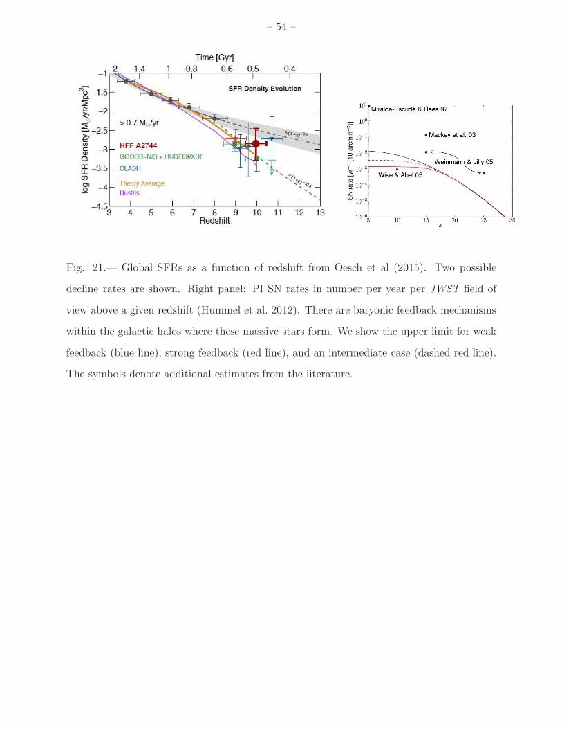
– 54 –

Fig. 21.— Global SFRs as a function of redshift from Oesch et al (2015). Two possible

decline rates are shown. Right panel: PI SN rates in number per year per JWST field of

view above a given redshift (Hummel et al. 2012). There are baryonic feedback mechanisms

within the galactic halos where these massive stars form. We show the upper limit for weak

feedback (blue line), strong feedback (red line), and an intermediate case (dashed red line).

The symbols denote additional estimates from the literature.