LiDAR Inertial Odometry Aided Robust LiDAR Localization System inChanging City Scenes

Wendong Ding, Shenhua Hou, Hang Gao, Guowei Wan, Shiyu Song1

Abstract— Environmental fluctuations pose crucial challengesto a localization system in autonomous driving. We present arobust LiDAR localization system that maintains its kinematicestimation in changing urban scenarios by using a deadreckoning solution implemented through a LiDAR inertialodometry. Our localization framework jointly uses informationfrom complementary modalities such as global matching andLiDAR inertial odometry to achieve accurate and smooth local-ization estimation. To improve the performance of the LiDARodometry, we incorporate inertial and LiDAR intensity cues intoan occupancy grid based LiDAR odometry to enhance frame-to-frame motion and matching estimation. Multi-resolutionoccupancy grid is implemented yielding a coarse-to-fine ap-proach to balance the odometry’s precision and computationalrequirement. To fuse both the odometry and global matchingresults, we formulate a MAP estimation problem in a posegraph fusion framework that can be efficiently solved. Aneffective environmental change detection method is proposedthat allows us to know exactly when and what portion ofthe map requires an update. We comprehensively validate theeffectiveness of the proposed approaches using both the Apollo-SouthBay dataset and our internal dataset. The results confirmthat our efforts lead to a more robust and accurate localizationsystem, especially in dynamically changing urban scenarios.

I. INTRODUCTION

Transportation of people and goods in the last hundredyears has changed at a drastic pace. This growth potentialin the industry attracted the attention of technology expertswho sought to solve this complex yet promising problem.More recently, disruptive technological concepts like ride-sharing and autonomous delivery are propelling this industryforward, like autonomous driving [1]. One of the primaryrequirements of an autonomous system is a defined mappedarea and in order to navigate autonomously, the prevalentapproach requires precise localization. But precise localiza-tion systems are not only complex but are also difficult toimplement in a dynamically changing environment. Previousworks [2], [3], [4], [5] have demonstrated that some specificchanges in the environment, e.g. road repavements, puddles,snowdrifts, can be overcome using existing technologies.However, it is still one of the most challenging issues thatcauses the failure of the vehicle’s localization module whichis based on matching online sensor measurements.

In this work, we seek to integrate a LiDAR inertialodometry (LIO) together with our matching based global

*This work is supported by Baidu Autonomous Driving TechnologyDepartment (ADT) in conjunction with the Apollo Project. Natasha Dsouzahelped with the text editing and proof reading.

The authors are with Baidu ADT, {dingwendong, houshenhua,gaohang04, wanguowei, songshiyu}@baidu.com.

1Author to whom correspondence should be addressed, E-mail:songshiyu@baidu.com

Day of Test Day of MapA B

C D E

0 1

Fig. 1: Online LiDAR data (brown) and the submap (occupancyprobability: blue/green/yellow) built by the LiDAR inertial odom-etry is shown on the left of the top panel. The prebuilt localizationmap marked with the probability of how likely change exists in eachcell estimated by the environmental change detection module isshown at the bottom right of the top panel. Bottom panel: zoomed-in view of an intersection where metal walls were recently removed.(A) and (B) comparison of the scene at different times. (C) visualcomparison of localization results: green car (w/ LIO) vs red (w/oLIO) vs blue (ground truth). (D) zoomed-in view of the changedetection results. (E) Updated map by merging new LiDAR scans.

LiDAR localization module. Both the measurements fromthe two modules are jointly fused in a pose graph opti-mization framework. Given the fact that map matching andodometry are complementary methods, it allows us to delivera robust localization system that can overcome temporaryenvironmental changes or map errors in general as shown inFigure 1, and at the same time consistently provide preciseglobal localization results.

To summarize, our main contributions are:

• A joint framework for vehicle localization that adap-tively fuses global matching and local odometry cues,which effectively shields our system from their failurein changing urban scenes.

• A LiDAR inertial odometry that tightly couples LiDAR

and inertial measurements and incorporates both theoccupancy and LiDAR intensity cues to provide realtime accurate state estimation.

• A robust vehicle localization system that has beenrigorously tested daily in crowded and busy urbanstreets demonstrating its robustness in challenging anddynamically changing environment.

II. RELATED WORK

Long-term Localization Building a 7 days 24 hours all-weather localization system is, by all means, a challengingtask that has received significant attention in recent years. J.Levinson et al. [6] showed that the less reflectance causedby wet road surface can be adjusted by normalizing thebrightness and standard deviation for each LiDAR scan. R.Wolcott et al. [2], [3] demonstrated a robust LiDAR local-ization system that can survive through road repavement andsnowfall by introducing a multiresolution Gaussian mixturerepresentation in the map. Wan et al. [5] showed that theLiDAR localization system successfully passed a challengingroad section with newly built walls and repaved road byincorporating the altitude cues. M. Aldibaja et al. [4] enhancethe robustness of their localization system by introducingprincipal component analysis (PCA) and edge profiles, espe-cially during rainy or snowy days. While these works focuson solving specific problems using niche technologies, ourwork seeks to have a more general solution by adaptivelyfusing the complementary cues from the odometry and theglobal matching module. Other works [7], [8], [9], [10],[11] address a similar long-term localization problem butuse vision sensors that are brittle to the scene’s appearancechange caused by time, light or weather.

LiDAR Inertial Odometry There is a lot of literatureaddressing the LiDAR odometry/SLAM problem [12], [13],[14], [15], [16], [17], [18], [19], [20], [21], [22], [23], [24].Inertial measurements help solve the problem by providingprior estimation and compensating the motion distortion [14],[18], [17], [19], building tighter local motion constraints[18] or further establishing a tightly-coupled odometry [23],[24]. In this work, we follow Hess’s work [13] and integratean occupancy grid based LiDAR inertial odometry into ourlocalization framework because of its similar map represen-tation to our global matching module and its compatibilityto multiple laser scanners. Inspired by previous works, theusage of inertial sensors and other extensions are introducedfor performance improvement.

Localization Fusion Methods There are several methodsrelated to the fusion of estimation from different sensors ormethods. One important category is loosely-coupled fusion.Methods [25], [5], [26] leverage error-state Kalman filterand loosely fuse the pose estimation from different methods.Instead of using a Kalman filter, similar to [26], our methodutilizes a graph-based fusion framework, which is known tooutperform filtering methods with better accuracy per unit ofcomputing time [27], [28]. A. Soloviev [29] demonstrates atightly-coupled navigation system fusing GNSS, LiDAR andinertial measurements.

Histogram FilterGlobal Matching

LiDAR Global Matching(LGM)

Prebuilt Localization Map

Sliding Window Optimization

Pose Graph Fusion(PGF)

SubmapProjection

Env. Change Detect(ECD)

Change Detection

MotionCompensation

IMU

LIDAR

Pre-Process

Submap Update

LiDAR Inertial Odometry(LIO)

IMUIntegration

Multi-ResolutionCloud

Scan Matching Global Local Transform

Fig. 2: The architecture of the proposed LiDAR inertial odometryaided LiDAR localization system with an environmental changedetection module.

III. METHOD

This section describes the architecture of the proposedLiDAR localization framework designed in detail as shownin Figure 2. Our system consists of four modules: LiDARinertial odometry (LIO), LiDAR global matching (LGM),pose graph based fusion (PGF) and environmental changedetection (ECD). We build our system by following the latestLiDAR localization work by G. Wan et al. [5], and leveragingit as a submodule, the LGM, in our framework. It is a globallocalization method that matches online LiDAR scans againsta pre-built map, and conducts a 3 DoF (x, y, yaw) estimation.The other 3 DoF (roll, pitch, altitude) can be estimated byreading IMU gravity measurements and a digital elevationmodel (DEM) map, once we successfully locate horizontally.The other two modules, LIO and PGF, are formulated interms of solving different maximum a posteriori probability(MAP) estimation problems.

The MAP estimation in this work leads to a nonlinearoptimization problem defined usually in a sliding windowconsidering a window of the latest measurements. Let Kdenote the set of all frames in a window. The set ofstates and measurements in a sliding window are denotedas X = {xk}k∈K and Z = {zk}k∈K, respectively. Thestate of frame k is represented by the orientation, position,velocity and IMU biases, xk = [ωk, tk,vk,bk]. ωk is theLie algebra usually denoted as so(3). Rk = Exp(ωk) andthe pose (Rk, tk) belong to the Special Orthogonal GroupSO(3) and the Special Euclidean Group SE(3) respectively.Exp() and Log() are the exponential and logarithmic mapassociating so(3) → SO(3) and SO(3) → so(3). Velocitiesare represented by vectors, i.e., vk ∈ R3. IMU biases can befurther written as bk = [bak,b

gk], where bak,b

gk ∈ R3 are the

accelerometer and gyroscope bias, respectively.

A. LiDAR Inertial Odometry

The LiDAR inertial odometry plays an essential role in oursystem in promoting localization performance in challengingcircumstances, for example, map expiration or environmentalchange due to road construction or severe weather. LiDARodometry estimates relative poses between frames and si-multaneously helps us build a local map, called a submap.This submap is always up-to-date, continuously updated witheach new LiDAR scan. Our system takes advantage of the

submap, smoothes the estimated trajectory, and also ensuresthe system reliability in extreme circumstances.

Our LiDAR inertial odometry implementation follows W.Hess’s work [13], but with a number of important exten-sions to improve its accuracy. Firstly, the method of the3D occupancy grid is used instead of 2D to achieve afull 6 DoF odometry. This extension naturally allows itsapplication in a three-dimensional environment, such as aparking structure or an overpass, and simplifies the under-mentioned IMU pre-integration. Secondly, important inertialcues are incorporated to provide motion prediction andrelative constraints between frames. More importantly, theincorporation of the inertial cues allows us to implement themotion compensation for the distorted LiDAR scans causedby the moving platform. In order to make the computingtime non-intractable, we adopt pre-integration of the inertialmeasurements introduced by [30] in our implementation.Thirdly, in consideration of the rich information from lane orroad surface markers in these scenarios, the LiDAR intensitycues are incorporated during the occupancy grid registrationas complementary to the occupancy probability of eachgrid cell. It provides valuable texture information of theenvironment. Finally, we apply a coarse-to-fine manner whilesolving the non-linear optimization problem by introducingmulti-resolution into our occupancy grid implementation.It not only helps the grid registration converge but alsokeeps the computational requirement at bay, validated byexperimental results in Section IV-C.

We formulate the LiDAR inertial odometry as a MAPestimation problem. The posterior probability of the statexLk , given the previous state xLk−1, the submap Sk−1 updateduntil the recent frame k − 1, and the measurements zk, is

P (xLk |zk,xLk−1,Sk−1) ∝ P (zPk |xLk ,Sk−1)

P (zIk|xLk ,xLk−1),(1)

where zk = {zPk , zIk}, zPk and zIk are the point cloud andinertial measurement, respectively. The superscript L denotesthat the state xLk is expressed in the local frame defined bythe submap and odometry.

Under the assumption of zero-mean Gaussian-like prob-ability, the likelihood of the measurements are defined bybuilding the cost functions as:

P (zIk|xLk ,xLk−1) ∝ exp−1

2‖rIk‖2ΛI

k, (2)

where ‖r‖2Λ = rTΛ−1r and

P (zPk |xLk ,Sk−1) ∝∏i

∏j

exp− 1

2σ2oi

‖SSOP‖2

∏i

∏j

exp− 1

2σ2ri

‖SSID‖2.(3)

The Equation 2 is calculated according to the pre-integration method. Please refer to [30] for details. TheSum of Squared Occupancy Probability) SSOP and Sum of

Squared Intensity Difference) SSID represent the occupancygrid probability and the LiDAR intensity cost, respectively,defined as: {

SSOP = 1− P (s)

SSID =us−I(pj)

σs.

(4)

Given a LiDAR point pj ∈ R3, a submap with resolutioni, and a pose state xLk = [Rk, tk], the hit cell s in thesubmap can be found. P (s) is the occupancy probabilityof the hit cell in the submap at the desired resolution i.This occupancy probability is maintained by keep insertingnew LiDAR scans into the submap after we maximize theposterior P (xLk |zk,xLk−1,Sk−1). This incremental upgradingproblem is addressed by the binary Bayesian filter using theinverse measurement model and the log odds ratio introducedin [31]. I(pj) is the LiDAR intensity of the point pj . usand σs are the mean and variance value of the LiDARintensity of the hit cell, respectively. To better ensure theregistration performance, we use cubic interpolation to obtainthe probability and the intensity values from the submap. Thevariance σoi and σri are used to weight the probability andintensity terms in the optimization at different resolutions ofthe submap.

The MAP estimate corresponds to the minimum of thenegative log-posterior and the latter can be written as a sumof squared residual errors, yielding a non-linear least squaresoptimization problem. It can be minimized using iterativealgorithms (e.g. Levenberg-Marquardt, Gauss-Newton), im-plemented in solvers, for example, Ceres [32].

B. Pose Graph Fusion

While a LiDAR inertial odometry can provide good rel-ative constraints in the local frame, we still need globalconstraints to achieve global localization. The LGM mod-ule furnishes our system with global cues and our LGMimplementation follows [5]. These complementary local andglobal cues are jointly optimized in a pose graph based fusionframework introduced in this section.

We formulate this fusion problem as a MAP estimationand factorize the posterior probability assuming uniformprior distribution as:

P (X|Z) ∝∏k,s

P (zOks|xLk ,xSs )∏k

P (zIk|xLk ,xLk−1)∏k

P (zGk |xLk ,xGL ).(5)

The factorization can be visualized as a Bayesian networkshown in Figure 3. If we assume zero-mean Gaussian-likeprobability, the likelihoods of the measurements can bedefined as:

P (zOks|xLk ,xSs ) ∝ exp− 12‖r

Oks‖2ΛO

P (zIk|xLk ,xLk−1) ∝ exp− 12‖r

Ik‖2ΛI

k

P (zGk |xLk ,xGL ) ∝ exp− 12‖r

Gk ‖2ΛG

k,

(6)

L L L L L L L

Prebuilt Localization Map

LiDAR LocalFrame PoseL

S S

Bias/Velocity

S Submap Pose

Global Posemeasurement

Local Frame

Global Frame

IMUmeasurement

Local GlobalTransform

G

LiDAR SubmapRelative Constraints

G

Fig. 3: The Bayesian network of the joint fusion problem. Statesand measurements are plotted in different colors. The factorizationof the Bayesian network assumes uniform prior distribution.

where rOks, rIk and rGk are the odometry, inertial and global

residuals, respectively.In our fusion framework, we maintain a local frame xLk

and a global state variable xGL , which transfers xLk to theglobal frame. If we define xLk = [RL

k , tLk ], xGL = [RG

L , tGL ],

and the global pose measurements zGk = [RGk , t

Gk ] output

by the LGM module [5], accordingly, we have the globalresidual cost as (rGk )T = [LogT (RrG), tTrG], where:

[RrG trG0 1

]=

[RG

k tGk0 1

]−1 [RG

L tGL0 1

] [RL

k tLk0 1

]. (7)

With regard to the covariance ΛGk in the global residual,we write it as

ΛGk = diag(ΛGω ,Λ

Ghk ,ΛGz ), (8)

where the rotation and the altitude covariance, ΛGω ∈R3×3 and ΛGz ∈ R1×1, respectively, are constant diagonalmatrices since our LGM module only estimates the hori-zontal localization uncertainty using a 2D histogram filteras discussed in [5]. As shown by Equation 12 from [5], thehorizontal matching covariance matrix ΛGh

k ∈ R2×2 is calcu-lated for each frame k accordingly. Note that the estimationuncertainty introduced here is critical to the performance ofthe localization system, yielding an adaptive fusion.

Concerning the odometry residual cost, we keep terminat-ing old and creating new submaps as our LiDAR odometrypropagates. The relative pose constraints zOks between thelocal frame and the submap output by the LIO module areestablished and saved in the life cycle of the sliding window.

Similarly, if we define the submap poses xSs = [RSs , t

Ss ],

and zOks = [ROks, t

Oks], we have the odometry residual cost as

(rOks)T = [LogT (RrO), tTrO], where

[RrO trO0 1

]=

[RO

ks tOks0 1

]−1 [RS

s tSs0 1

]−1 [RL

k tLk0 1

]. (9)

In terms of the covariance ΛO in the odometry residual,we use a globally constant diagonal matrix across all framesand submaps assuming the estimation uncertainty is evenlydistributed among all frames.

The pre-integration of the inertial constraints are treatedin the same way as introduced in [30]. The non-linear leastsquares optimization is solved using the Ceres solver [32].

C. Environmental Change Detection

It is known that the LGM module relies on the freshnessof the prebuilt localization map. We always seek to findout when it is time to update our localization map. Thesubmaps generated in the LIO module not only can beused to estimate the relative pose between frames but alsocan be used to detect the environmental changes. This iscrucial for a localization system, especially if we practicallyconsider its commercial deployment. Therefore, we buildan environmental change detection (ECD) module basedon the submaps from our LIO. Firstly, we project our 3Dmulti-resolution submap onto the ground plane similar to thelocalization map building procedures in [6], [2], [5]. Then, a2D submap in the same representation format to our prebuiltlocalization map is obtained. Given the localization outputsof the system, we can overlay the submap S onto the prebuiltmapM and the occurrence of the environmental change canbe determined by comparing them cell by cell. Let us denoteus, σs, as, um, σm, and am as the intensity mean, intensityvariance, and altitude mean of a pair of corresponding cellsin the submap and the prebuilt map, respectively. We have

zs(r) =(us − um)2(σ2

s + σ2m)

σ2sσ

2m

zs(a) = (as − am)2,

(10)

where zs(r) and zs(a) evaluate how likely the environmentalchange exists in the cell.

We formulate the occurrence of the change within eachcell as a binary state estimation problem addressed by thebinary Bayesian filter. Similar to the occupancy grid update,if several vehicles have passed the same area multiple timesgenerating more submaps, we can similarily update theprobability of the change occurrence by using a binaryBayesian filter [31]. If we denote the occurrence of thechange within a cell as a binary state variable ds, the inversemeasurement model for updating the binary Bayesian filtercan be defined as:

P (ds|zs) = ηP (ds|zs(r))γP (ds|zs(a))1−γ , (11)

where γ is a dynamic weighting parameter that balances theweights of the intensity and altitude cues. We can furtherdefine their inverse measurement model by normalizing zs(r)and zs(a) within the submap as:

{P−1(ds|zs(r)) = 1 + exp (−β1( zs(r)−us(r)

σs(r) − θ1))

P−1(ds|zs(a)) = 1 + exp (−β2( zs(a)−us(a)σs(a) − θ2)),

(12)where us(r), us(a), σs(r), σs(a) are the mean and varianceof zs(r) and zs(a), respectively, aggregated in a submap. βand θ are parameters set empirically.

IV. EXPERIMENTAL RESULTS

A. Platforms and Datasets

Our system has been extensively tested in real-worlddriving scenarios primarily using two datasets, our internaldataset, and the Apollo-SouthBay dataset [33], [34]. Whilethe Apollo-SouthBay dataset was collected in San FranciscoBay Area, United States, covering a driving distance of380.5km, our internal dataset includes the various challeng-ing urban scenarios in Beijing, China, especially the oneswith map errors or environmental changes, such as mapexpiration (gradual environment change), road construction,closed lanes, dense traffic and so on. These challenges mightbe unusual or can be avoided by altering the operationalroutes in other parts of the world, but are actually quitecommon and happen daily in different parts of Beijing, thecapital city of one of the largest developing countries - China.

Our vehicle platform is equipped with a Velodyne HDL-64E 360◦ LiDAR and a NovAtel PwrPak7D-E1 GNSS RTKreceiver integrated with dual antennas and an Epson EG320NIMU. These sensors are all mounted on a Lincoln MKZvehicle. The ground truth poses used in the evaluation aregenerated using offline LiDAR SLAM methods typicallyformulated as a large-scale global least-square optimizationproblem, which are beyond the scope of this work.

B. Localization Performance

The localization performance is compared against Wan etal. [5], in which 2-System mode is applied because LiDAR-based localization is our primary focus. Our quantitativeanalysis includes horizontal and heading errors with bothRMS and maximum values. The horizontal errors are fur-ther decomposed to longitudinal (Long.) and lateral (Lat.)directions in Table II. The percentages of frames where thesystem achieves better than 0.1m, 0.2m, 0.3m or 0.1◦ inhorizontal or heading estimations are shown in the tables.

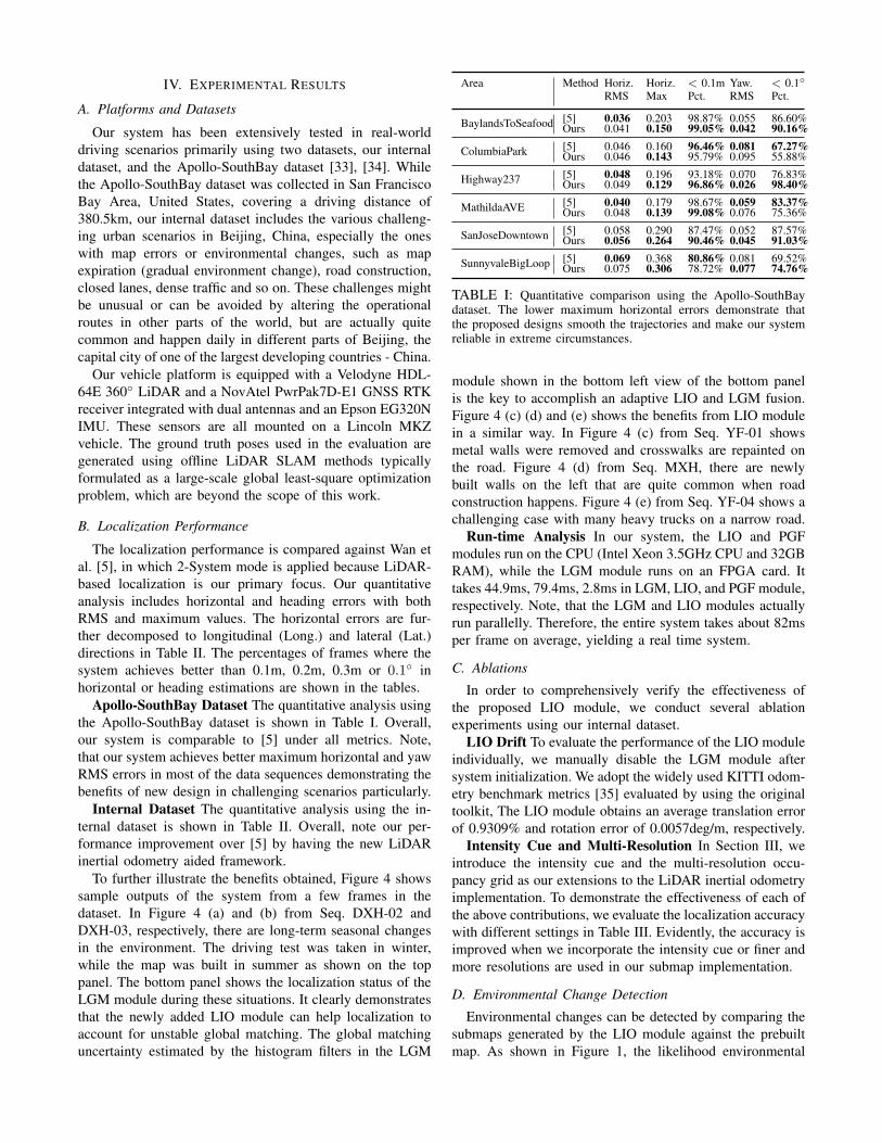
Apollo-SouthBay Dataset The quantitative analysis usingthe Apollo-SouthBay dataset is shown in Table I. Overall,our system is comparable to [5] under all metrics. Note,that our system achieves better maximum horizontal and yawRMS errors in most of the data sequences demonstrating thebenefits of new design in challenging scenarios particularly.

Internal Dataset The quantitative analysis using the in-ternal dataset is shown in Table II. Overall, note our per-formance improvement over [5] by having the new LiDARinertial odometry aided framework.

To further illustrate the benefits obtained, Figure 4 showssample outputs of the system from a few frames in thedataset. In Figure 4 (a) and (b) from Seq. DXH-02 andDXH-03, respectively, there are long-term seasonal changesin the environment. The driving test was taken in winter,while the map was built in summer as shown on the toppanel. The bottom panel shows the localization status of theLGM module during these situations. It clearly demonstratesthat the newly added LIO module can help localization toaccount for unstable global matching. The global matchinguncertainty estimated by the histogram filters in the LGM

Area Method Horiz.RMS

Horiz.Max

< 0.1mPct.

Yaw.RMS

< 0.1◦Pct.

BaylandsToSeafood [5] 0.036 0.203 98.87% 0.055 86.60%Ours 0.041 0.150 99.05% 0.042 90.16%

ColumbiaPark [5] 0.046 0.160 96.46% 0.081 67.27%Ours 0.046 0.143 95.79% 0.095 55.88%

Highway237 [5] 0.048 0.196 93.18% 0.070 76.83%Ours 0.049 0.129 96.86% 0.026 98.40%

MathildaAVE [5] 0.040 0.179 98.67% 0.059 83.37%Ours 0.048 0.139 99.08% 0.076 75.36%

SanJoseDowntown [5] 0.058 0.290 87.47% 0.052 87.57%Ours 0.056 0.264 90.46% 0.045 91.03%

SunnyvaleBigLoop [5] 0.069 0.368 80.86% 0.081 69.52%Ours 0.075 0.306 78.72% 0.077 74.76%

TABLE I: Quantitative comparison using the Apollo-SouthBaydataset. The lower maximum horizontal errors demonstrate thatthe proposed designs smooth the trajectories and make our systemreliable in extreme circumstances.

module shown in the bottom left view of the bottom panelis the key to accomplish an adaptive LIO and LGM fusion.Figure 4 (c) (d) and (e) shows the benefits from LIO modulein a similar way. In Figure 4 (c) from Seq. YF-01 showsmetal walls were removed and crosswalks are repainted onthe road. Figure 4 (d) from Seq. MXH, there are newlybuilt walls on the left that are quite common when roadconstruction happens. Figure 4 (e) from Seq. YF-04 shows achallenging case with many heavy trucks on a narrow road.

Run-time Analysis In our system, the LIO and PGFmodules run on the CPU (Intel Xeon 3.5GHz CPU and 32GBRAM), while the LGM module runs on an FPGA card. Ittakes 44.9ms, 79.4ms, 2.8ms in LGM, LIO, and PGF module,respectively. Note, that the LGM and LIO modules actuallyrun parallelly. Therefore, the entire system takes about 82msper frame on average, yielding a real time system.

C. Ablations

In order to comprehensively verify the effectiveness ofthe proposed LIO module, we conduct several ablationexperiments using our internal dataset.

LIO Drift To evaluate the performance of the LIO moduleindividually, we manually disable the LGM module aftersystem initialization. We adopt the widely used KITTI odom-etry benchmark metrics [35] evaluated by using the originaltoolkit, The LIO module obtains an average translation errorof 0.9309% and rotation error of 0.0057deg/m, respectively.

Intensity Cue and Multi-Resolution In Section III, weintroduce the intensity cue and the multi-resolution occu-pancy grid as our extensions to the LiDAR inertial odometryimplementation. To demonstrate the effectiveness of each ofthe above contributions, we evaluate the localization accuracywith different settings in Table III. Evidently, the accuracy isimproved when we incorporate the intensity cue or finer andmore resolutions are used in our submap implementation.

D. Environmental Change Detection

Environmental changes can be detected by comparing thesubmaps generated by the LIO module against the prebuiltmap. As shown in Figure 1, the likelihood environmental

Scenes Dist.(km)

Method Horiz.RMS

Horiz.Max

Long.RMS

Long.Max

Lat.RMS

Lat.Max

< 0.1mPct.

< 0.2mPct.

< 0.3mPct.

DXH-01 11.03 [5] 0.056 0.803 0.037 0.311 0.034 0.740 91.42% 99.08% 99.50%Ours 0.048 0.472 0.029 0.196 0.031 0.459 95.31% 99.07% 99.44%

DXH-02 1.693 [5] 0.087 0.870 0.052 0.666 0.063 0.735 76.67% 94.02% 99.44%Ours 0.074 0.260 0.041 0.142 0.054 0.256 81.49% 94.31% 100.0%

DXH-03 1.615 [5] 0.093 0.402 0.080 0.401 0.036 0.202 61.54% 99.20% 99.93%Ours 0.085 0.168 0.076 0.167 0.033 0.111 72.76% 100.0% 100.0%

MXH 2.563 [5] 0.086 1.669 0.047 1.023 0.064 1.421 68.75% 99.15% 99.18%Ours 0.069 0.223 0.036 0.126 0.052 0.223 89.52% 99.52% 100.0%

YZ-01 7.263 [5] 0.070 2.841 0.045 0.233 0.046 2.836 85.43% 99.12% 99.65%Ours 0.063 0.313 0.047 0.184 0.034 0.294 91.66% 99.26% 99.96%

YZ-02 4.638 [5] 0.069 0.336 0.039 0.194 0.050 0.316 77.61% 99.61% 99.92%Ours 0.062 0.274 0.040 0.169 0.041 0.251 86.43% 99.60% 100.0%

YZ-03 2.567 [5] 0.064 0.235 0.046 0.190 0.037 0.228 83.88% 99.71% 100.0%Ours 0.059 0.250 0.043 0.250 0.032 0.186 92.04% 99.92% 100.0%

YZ-04 0.911 [5] 0.177 1.111 0.129 0.982 0.105 1.010 53.95% 80.16% 84.45%Ours 0.085 0.365 0.065 0.186 0.042 0.361 68.63% 95.53% 98.44%

TABLE II: Quantitative comparison using our internal dataset. The benefits of the LiDAR inertial odometry are clearly visible from thelocalization accuracy enhancement.

(a)

Day of Test

Day of Map

(b)

Day of Test

Day of Map

(c)

Day of Test

Day of Map

(e)

Day of Test

(d)

Day of Test

Day of Map

Fig. 4: Top panel: (a) and (b) long-term seaonal changes from DXH-02 and DXH-03, respectively. The driving test was taken in winter,while the map was built in summer. (c) metal walls were removed and crosswalks are repainted from YF-01. (d) new walls were builton the left from MXH. (e) dynamic objects, such as many heavy trucks, on a narrow road from YF-04. Bottom panel: visual comparisonof localization results. Green cars are the fused results estimated in our joint optimization framework. Red cars are the results generatedonly by the LGM module. Blue cars are the ground truth. When the green cars perfectly overlap with the blue ones (can not be seen),the results are accurate. The bottom left view in the bottom panel depicts the histogram filter response in the LGM module.

Method Translation (%) Rotation (deg/m)

Ours w/ Intensity 0.9309 0.0057{0.125, 0.25, 0.6, 1.2} 0.9498 0.0057{0.125} 0.9520 0.0058{0.6} 1.7637 0.0102

TABLE III: Comparison w/o the intensity cue or multi-resolution.Note that using coarser or single resolution grid gives worse results.Ours with the intensity cue yields the best odometry accuracy.

change exists in each map cell is marked on the map usinga rainbow scale bar. An intersection where metal walls wererecently removed is zoomed-in to further demonstrate thedetails of environmental change detection results.

V. CONCLUSION

We have presented a robust LiDAR localization frame-work, designed for autonomous driving applications, espe-

cially countering the localization challenges in changing cityscenes. The proposed method utilizes a pose graph basedfusion framework adaptively incorporating results from boththe LiDAR inertial odometry and global matching modules.It has been shown that the newly added LiDAR inertialodometry module can effectively aid the localization systemin the prevention of localization errors caused by the globalmatching failure. We also propose an environmental changedetection method to find out when and what portion of themap should be promptly updated in order to reliably supportthe daily operation of our large autonomous driving fleet incrowded city streets, despite road construction that may haveoccurred from time to time. These distinct advantages makeour system quite attractive to real commercial deployment.In a further extension of this work, we plan to explorelearning-based environmental change detection methods forcomparison.

REFERENCES

[1] “Baidu Apollo open platform,” http://apollo.auto/.[2] R. W. Wolcott and R. M. Eustice, “Fast LiDAR localization using

multiresolution gaussian mixture maps,” in Proceedings of the IEEEInternational Conference on Robotics and Automation (ICRA), 2015,pp. 2814–2821.

[3] ——, “Robust LiDAR localization using multiresolution gaussianmixture maps for autonomous driving,” The International Journal ofRobotics Research (IJRR), vol. 36, no. 3, pp. 292–319, 2017.

[4] M. Aldibaja, N. Suganuma, and K. Yoneda, “Robust intensity-basedlocalization method for autonomous driving on snow-wet road sur-face,” Transactions on Industrial Informatics, vol. 13, no. 5, pp. 2369–2378, 2017.

[5] G. Wan, X. Yang, R. Cai, H. Li, Y. Zhou, H. Wang, and S. Song,“Robust and precise vehicle localization based on multi-sensor fusionin diverse city scenes,” in Proceedings of the IEEE InternationalConference on Robotics and Automation (ICRA), 2018, pp. 4670–4677.

[6] J. Levinson, M. Montemerlo, and S. Thrun, “Map-based precisionvehicle localization in urban environments.” in Proceedings of theRobotics: Science and Systems (RSS), vol. 4, 2007, p. 1.

[7] C. McManus, W. Churchill, W. Maddern, A. D. Stewart, and P. New-man, “Shady dealings: Robust, long-term visual localisation usingillumination invariance,” in Proceedings of the IEEE InternationalConference on Robotics and Automation (ICRA), 2014, pp. 901–906.

[8] C. Linegar, W. Churchill, and P. Newman, “Work smart, not hard:Recalling relevant experiences for vast-scale but time-constrainedlocalisation,” in Proceedings of the IEEE International Conferenceon Robotics and Automation (ICRA), 2015, pp. 90–97.

[9] ——, “Made to measure: Bespoke landmarks for 24-hour, all-weatherlocalisation with a camera,” in Proceedings of the IEEE InternationalConference on Robotics and Automation (ICRA), 2016, pp. 787–794.

[10] M. Burki, I. Gilitschenski, E. Stumm, R. Siegwart, and J. Nieto,“Appearance-based landmark selection for efficient long-term visuallocalization,” in Proceedings of the IEEE International Conference onIntelligent Robots and Systems (IROS), 2016, pp. 4137–4143.

[11] T. Sattler, W. Maddern, C. Toft, A. Torii, L. Hammarstrand, E. Sten-borg, D. Safari, M. Okutomi, M. Pollefeys, J. Sivic et al., “Bench-marking 6DOF outdoor visual localization in changing conditions,” inProceedings of the IEEE Conference on Computer Vision and PatternRecognition (CVPR), 2018, pp. 8601–8610.

[12] J. Zhang and S. Singh, “LOAM: LiDAR odometry and mapping inreal-time.” in Proceedings of the Robotics: Science and Systems (RSS),vol. 2, 2014, p. 9.

[13] W. Hess, D. Kohler, H. Rapp, and D. Andor, “Real-time loop closurein 2D LiDAR SLAM,” in Proceedings of the IEEE InternationalConference on Robotics and Automation (ICRA), 2016, pp. 1271–1278.

[14] J. Zhang and S. Singh, “Low-drift and real-time LiDAR odometry andmapping,” Autonomous Robots, vol. 41, no. 2, pp. 401–416, 2017.

[15] C. Park, S. Kim, P. Moghadam, C. Fookes, and S. Sridharan, “Prob-abilistic surfel fusion for dense LiDAR mapping,” in Proceedings ofthe IEEE International Conference on Computer Vision (ICCV), 2017,pp. 2418–2426.

[16] J. Behley and C. Stachniss, “Efficient surfel-based SLAM using3D laser range data in urban environments,” in Proceedings of theRobotics: Science and Systems (RSS), 2018.

[17] D. Droeschel and S. Behnke, “Efficient continuous-time SLAM for3D LiDAR-based online mapping,” in Proceedings of the IEEEInternational Conference on Robotics and Automation (ICRA), 2018,pp. 1–9.

[18] C. Park, P. Moghadam, S. Kim, A. Elfes, C. Fookes, and S. Sridharan,“Elastic LiDAR fusion: Dense map-centric continuous-time SLAM,”in Proceedings of the IEEE International Conference on Robotics andAutomation (ICRA), 2018, pp. 1206–1213.

[19] T. Shan and B. Englot, “LeGO-LOAM: Lightweight and ground-optimized LiDAR odometry and mapping on variable terrain,” inProceedings of the IEEE/RSJ International Conference on IntelligentRobots and Systems (IROS), 2018, pp. 4758–4765.

[20] J.-E. Deschaud, “IMLS-SLAM: Scan-to-model matching based on3D data,” in Proceedings of the IEEE International Conference onRobotics and Automation (ICRA), 2018, pp. 2480–2485.

[21] Q. Li, S. Chen, C. Wang, X. Li, C. Wen, M. Cheng, and J. Li, “LO-Net: Deep real-time LiDAR odometry,” in Proceedings of the IEEE

Conference on Computer Vision and Pattern Recognition(CVPR),2019, pp. 8473–8482.

[22] Y. Cho, G. Kim, and A. Kim, “DeepLO: Geometry-Aware DeepLiDAR Odometry,” arXiv preprint arXiv:1902.10562, 2019.

[23] H. Ye, Y. Chen, and M. Liu, “Tightly coupled 3D lidar inertialodometry and mapping,” arXiv preprint arXiv:1904.06993, 2019.

[24] C. Qin, H. Ye, C. E. Pranata, J. Han, and M. Liu, “LINS: A LiDAR-Inerital state estimator for robust and fast navigation,” arXiv preprintarXiv:1907.02233, 2019.

[25] Y. Gao, S. Liu, M. Atia, and A. Noureldin, “INS/GPS/LiDAR inte-grated navigation system for urban and indoor environments usinghybrid scan matching algorithm,” Sensors, vol. 15, no. 9, pp. 23 286–23 302, 2015.

[26] H. Liu, Q. Ye, H. Wang, L. Chen, and J. Yang, “A precise and robustsegmentation-based LiDAR localization system for automated urbandriving,” Remote Sensing, vol. 11, no. 11, p. 1348, 2019.

[27] F. Dellaert and M. Kaess, “Square root SAM: Simultaneous local-ization and mapping via square root information smoothing,” TheInternational Journal of Robotics Research(IJRR), vol. 25, no. 12,pp. 1181–1203, 2006.

[28] H. Strasdat, J. Montiel, and A. J. Davison, “Real-time monocularSLAM: Why filter?” in Proceedings of the IEEE International Con-ference on Robotics and Automation (ICRA), 2010, pp. 2657–2664.

[29] A. Soloviev, “Tight coupling of GPS, laser scanner, and inertialmeasurements for navigation in urban environments,” in Proceedingsof the IEEE/ION Position, Location and Navigation Symposium, 2008,pp. 511–525.

[30] C. Forster, L. Carlone, F. Dellaert, and D. Scaramuzza, “On-manifoldpreintegration for real-time visual–inertial odometry,” Transactions onRobotics, vol. 33, no. 1, pp. 1–21, 2017.

[31] S. Thrun, W. Burgard, and D. Fox, Probabilistic robotics. MIT press,2005.

[32] S. Agarwal, K. Mierle, and Others, “Ceres solver,” http://ceres-solver.org.

[33] W. Lu, Y. Zhou, G. Wan, S. Hou, and S. Song, “L3-Net: Towardslearning based LiDAR localization for autonomous driving,” in Pro-ceedings of the IEEE Conference on Computer Vision and PatternRecognition (CVPR), 2019, pp. 6389–6398.

[34] W. Lu, G. Wan, Y. Zhou, X. Fu, P. Yuan, and S. Song, “DeepVCP:An end-to-end deep neural network for point cloud registration,” inProceedings of the IEEE International Conference on Computer Vision(ICCV), 2019.

[35] A. Geiger, P. Lenz, and R. Urtasun, “Are we ready for autonomousdriving? the KITTI vision benchmark suite,” in Proceedings ofthe IEEE Conference on Computer Vision and Pattern Recognition(CVPR), 2012, pp. 3354–3361.