COMPARISON OF LIDAR AND

CONVENTIONAL MAPPING METHODS FOR

HIGHWAY CORRIDOR STUDIES

Sponsored byNational Consortium on Remote Sensing in Transportation for Infrastructure

University of California, Santa Barbara

Center for Transportation

Research and Education

CTRE

Final Report ● October 2002

The opinions, findings, and conclusions expressed in this publication are those of the authors and notnecessarily those of the sponsor.

CTRE’s mission is to develop and implement innovative methods, materials, and technologies forimproving transportation efficiency, safety, and reliability while improving the learning environment ofstudents, faculty, and staff in transportation-related fields.

COMPARISON OF LIDAR AND CONVENTIONAL MAPPING METHODS FOR

HIGHWAY CORRIDOR STUDIES

Principal Investigator Reginald Souleyrette

Associate Professor of Civil Engineering, Iowa State University Associate Director for Transportation Planning and Information Systems,

Center for Transportation Research and Education

Co-Principal Investigator Shauna Hallmark

Assistant Professor of Civil Engineering, Iowa State University Transportation Engineer, Center for Transportation Research and Education

Research Assistant

David Veneziano

Authors David Veneziano, Shauna Hallmark, and Reginald Souleyrette

Center for Transportation Research and Education Iowa State University

2901 South Loop Drive, Suite 3100 Ames, Iowa 50010-8634

Phone: 515-294-8103 Fax: 515-294-0467

www.ctre.iastate.edu

Final Report • October 2002

iii

Table of Contents 1. EXECUTIVE SUMMARY .............................................................................................1 2. INTRODUCTION .......................................................................................................... 3 3. PROJECT OVERVIEW ................................................................................................. 4

3.1 Scope of Work .........................................................................................................4 3.2 Expected Benefits ....................................................................................................4

4. BACKGROUND ............................................................................................................ 5 4.1 EDM (Total Station) ................................................................................................5 4.2 Real Time Kinematic Global Positioning System ...................................................6

4.2.1 Differential GPS..............................................................................................6 4.2.2 Kinematic GPS................................................................................................6

4.3 Photogrammetry.......................................................................................................7 4.3.1 Softcopy Photogrammetry...............................................................................7 4.3.2 Advantages and Disadvantages of Photogrammetry......................................7

4.4 LIDAR .....................................................................................................................8 4.4.1 Description of Technology..............................................................................8 4.4.2 LIDAR Errors................................................................................................10 4.4.3 Use of LIDAR in Transportation Applications .............................................10

5. STATE DOT LOCATION PROCESSES .................................................................... 14 5.1 Iowa Location Process ...........................................................................................14

5.1.1 Receipt of Project Assignment ......................................................................14 5.1.2 Project Management Team...........................................................................14 5.1.3 Highway Location Process ...........................................................................15

5.2 Virginia DOT Location Process.............................................................................18 5.3 New Mexico State Highway and Transportation Department Location Process ..22

6. EVALUATION OF ACCURACY ............................................................................... 25 6.1 Other Accuracy Studies .........................................................................................25 6.2 Description of Study Area .....................................................................................26 6.3 Photogrammetry.....................................................................................................26 6.4 Collection of LIDAR Data.....................................................................................27 6.4 GPS Data................................................................................................................28 6.5 Accuracy Comparison Methodology .....................................................................28

6.5.1 Direct Point Comparison..............................................................................28 6.5.2 Point Interpolation........................................................................................28 6.5.3 Grid Comparison ..........................................................................................29

6.6 Surface Comparison...............................................................................................29 6.7 Statistical Test........................................................................................................30

6.7.1 National Standards for Spatial Data Accuracy ............................................30 6.7.2 RMSE Test.....................................................................................................31

6.8 Results....................................................................................................................31 6.8.1 Using GPS as Control Points .......................................................................32 6.8.2 Using Photogrammetry as Control Points....................................................35

6.9 Study Limitations...................................................................................................39 6.10 Conclusions..........................................................................................................39

iv

7. OVERVIEW OF THE IOWA DOT EXPERIENCE WITH LIDAR FOR A HIGHWAY LOCATION STUDY ................................................................................... 40

7.1 Project Description.................................................................................................40 7.2 LIDAR Data Collection .........................................................................................42

7.2.1 Consultant Selection .....................................................................................42 7.2.2 Contract Development ..................................................................................42

7.3 Data Collection ......................................................................................................43 7.3.1 Early Problems .............................................................................................43 7.3.2 LIDAR Data Delivery ...................................................................................44

7.4 Current Status of U.S. 30 Project...........................................................................45 7.5 Preliminary Anticipated Results ............................................................................45 7.6 Anticipated Problems.............................................................................................45 7.7 Initial Conclusions .................................................................................................45

8. EVALUATION OF THE USE OF LIDAR IN HIGHWAY LOCATION STUDIES . 47 8.1 Existing Photogrammetric Data Collection Process at the Iowa DOT..................47 8.2 Proposed Integration Methodology of LIDAR with Photogrammetric Process....48 8.3 Integration of LIDAR into the Highway Location Process in Other States ..........52 8.4 Estimated Time and Cost Savings .........................................................................52

8.4.1 U.S. 30...........................................................................................................52 8.4.2 Iowa-1 ...........................................................................................................53

8.5 Conclusions............................................................................................................53 8.6 Disadvantages .......................................................................................................53 8.7 Future Research .....................................................................................................54

9. REFERENCES ............................................................................................................. 56

1

1. EXECUTIVE SUMMARY This report discusses the use of LIDAR derived surface terrain information to

locate (or determine location of) new or relocate existing transportation facilities. Terrain information is used both to construct and evaluate alternative routes and to create final design plans that optimize alignments and grades for the selected alternative. Currently, ground surveying and photogrammetric mapping are the methods used by state Departments of Transportation (DOTs) to acquire this data. Both methods are time and resource intensive since they require significant data collection and reduction to provide the level of detail necessary for facility location. In addition, these methods are limited by environmental factors, such as weather. Photogrammetric data collection is most constrained by these factors. Collection of the appropriate aerial imagery is often constrained to early spring or late fall so that data collection occurs under leaf-off conditions and the appropriate sun angle (above 30 degrees) with cloud-free skies. These requirements severely limit the available window during which imagery can be acquired, especially in northern climates. With conventional surveying, data collection occurs almost entirely in the field and may require that data collection personnel locate on or near heavily traveled roadways. Additionally, because of extensive in-field data collection, its use is impractical for sizeable projects. Field data collection for photogrammetry is less onerous, but once aerial imagery are obtained, a significant amount of processing is necessary before any useful terrain information is available. The result is the passage of a significant amount of time between project inception and final route selection, construction, and completion.

The use of light detection and ranging (LIDAR) to supplement the design process

is presented in this report. Early research results as well as surveyed literature indicate that LIDAR data cannot replace photogrammetric data in the final design stages of the highway location and design process. Results of the literature and this research also indicate that LIDAR accuracy is less consistent than indicated by vendors. Accuracy approached the vendor specified 15 cm vertical accuracy only under optimal conditions. A second preliminary conclusion is that LIDAR data are not yet accurate enough for final design and breaklines. Photogrammetric data are still required to produce highly accurate terrain models, as well as additional data, such as breaklines.

However, these limitations do not entirely prevent LIDAR data from being

utilized in the location and design process. The true potential of LIDAR in the process appears to be a supplemental form of data collection to photogrammetry. LIDAR could be collected for large area corridors, providing designers with the terrain information necessary to identify favorable alignments at earlier stages. Once such alignments have been identified, detailed photogrammetric data could then be produced for a lesser area. The result could be a significant savings in time and possibly money—through labor savings—using this modified data collection approach. This report is organized in the following manner. An introduction is provided in Section 2, and the scope of work presented in Section 3. Section 4 describes the LIDAR process and discusses LIDAR accuracies reported by other researchers. Section 5 lays out the Iowa DOT’s method for highway location and design and presents Virginia’s and

2

New Mexico’s processes. The sixth section presents results of accuracy comparisons between LIDAR, photogrammetry, and GPS. Section 7 describes the Iowa DOT’s experience contracting with a LIDAR vendor to collect surface terrain information from LIDAR. The last section discusses how LIDAR could fit into the highway location process given that it cannot yet take the place of photogrammetry.

3

2. INTRODUCTION

Surface terrain information is required to economically locate new or relocate existing transportation facilities. Terrain information is used both to construct and evaluate alternative routes and to create final design plans that optimize alignments and grades for the selected alternative. Currently, ground surveying and photogrammetric mapping are the methods used by state Departments of Transportation (DOTs) to acquire this data. Both methods are time and resource intensive since they require significant data collection and reduction to provide the level of detail necessary for facility location. In addition, these methods are limited by environmental factors, such as weather. Photogrammetric data collection is most constrained by these factors. Collection of the appropriate aerial imagery is often constrained to early spring or late fall so that data collection occurs under leaf-off conditions and the appropriate sun angle (above 30 degrees) with cloud-free skies. These requirements severely limit the available window during which imagery can be acquired, especially in northern climates. With conventional surveying, data collection occurs almost entirely in the field and may require that data collection personnel locate on or near heavily traveled roadways. Additionally, because of extensive in-field data collection, its use is impractical for sizeable projects. Field data collection for photogrammetry is less onerous, but once aerial imagery are obtained, a significant amount of processing is necessary before any useful terrain information is available. The result is the passage of a significant amount of time between project inception and final route selection, construction, and completion.

To reduce the time required to plan and design highway projects, highway

agencies have begun to streamline processes. In order to meet the extensive data requirements for environmental assessment and final design, some agencies have chosen to collect and process more terrain data and imagery products than they will ultimately need, in order to be able to rapidly respond to changing location decisions. While facilitating a smoother, faster planning process, the additional data collection and processing is expensive and time consuming. For example, a highway bypass study may require as many as 18 months of photogrammetric processing.

The existing process requires early collection and processing of data to support

final design. However, only the final design stages of project development may require the accuracies provided by conventional photogrammetric processing. Advanced methods of surface mapping, LIDAR, and digital photography may be used for preliminary planning and location issues, limiting expensive and time consuming photogrammetric work to the final alignment corridor. If LIDAR-developed terrain products and digital imagery are sufficient for planning stages, products could be delivered to planners and designers more rapidly and at lower costs. Once final alignment decisions are made, photogrammetric control and processing could be limited to an area perhaps one-fifth or smaller than the original location corridor. This scale of photogrammetric work could be completed in a short time at a much-reduced cost. In order for these savings to be realized, engineers and planners must be able to use the products and resulting designs must be of sufficient accuracy. This report discusses such a use of LIDAR data in the preliminary planning stages of highway corridor studies.

4

3. PROJECT OVERVIEW 3.1 Scope of Work

This research focused on determining whether the accuracy of LIDAR data is suitable for the needs of state DOTs for highway planning and design. In order to make this determination, LIDAR data were compared to photogrammetric data, which served as the “control”. Additional comparisons were made with independently collected GPS data to validate the accuracy of both LIDAR and photogrammetry. If LIDAR data proved to be accurate enough, it could serve as a supplemental form of data collection to photogrammetry in the preliminary stages of route location and design.

A second objective of this research was to determine how LIDAR data collection

fits into the highway location process. In order to determine how LIDAR can be integrated, this report presents documentation of existing location processes for several states, including Iowa, Virginia, and New Mexico.

To accomplish the objectives stated, the scope of research included the following:

• Identify current methodologies utilized by state DOTs for collecting terrain information and evaluate the advantages and disadvantages of each

• Document existing procedures of the Iowa DOT and additional DOTs for route location

• Document where the use of terrain data fits into the location process • Document the Iowa DOT’s experiences with LIDAR • Determine the elevational accuracy of LIDAR data collected during leaf-on

conditions in various types of terrain • Document surface types in which LIDAR performed well • Establish a methodology for implementing LIDAR data collection with

photogrammetric data collection • Evaluate the advantages and disadvantages of using LIDAR data collection (costs,

time savings, etc.)

To compare LIDAR accuracy, a study corridor was used. The corridor was selected for comparison in conjunction with the Photogrammetric Division of the Iowa DOT and was chosen from existing DOT projects that had been mapped within the last one to three years using conventional methods. The same corridor was then mapped with LIDAR. 3.2 Expected Benefits This research is expected to help transportation agencies determine if LIDAR data collected meets their accuracy needs by comparing the collected LIDAR with photogrammetry and GPS. This research is also expected to determine how LIDAR data collection can be integrated with existing techniques, namely photogrammetry, for expediting the location and design processes. Since LIDAR data can be quickly collected and produced for large areas, such data collection could be used to define narrow corridors for which highly accurate photogrammetry data could be collected and produced. By limiting the area for which time and labor intensive photogrammetry data are produced, projects could be completed in a timelier manner, producing cost savings.

5

4. BACKGROUND The following sections discuss data collection techniques for creation of surface

terrain models. Conventional methods are discussed as well as LIDAR. The Iowa DOT uses several methods for terrain data collection. They include electronic distance measurement devices (EDMs), real time kinematic global positioning systems (RTK GPS), and photogrammetry. 4.1 EDM (Total Station) EDMs were first introduced in the 1950s (Kavanagh 2001). Many different EDMs are available, but all operate in a similar fashion. A transmitter in the EDM transmits a light, laser, or radio beam to a reflector held at a point some distance from the device where distance measurement is desired. The reflector transmits the beam back to the transmitter, and the difference in phase between the transmitted and reflected wave is measured electronically to determine the distance between the transmitter and the reflector (Garber and Hoel 1997). When electronic theodolites are interfaced with these devices, they become electronic tachometer instruments, or Total Stations.

Total Stations are capable of measuring and recording horizontal and vertical angles as well as slope distances. The microprocessor contained in the Total Station unit is capable of determining a variety of information, including Cartesian coordinates (X,Y, Z), which define surface terrain. Some Total Stations are able to compute elevations at remote points (Kavanagh 2001). Total Stations are particularly useful in many types of surveys, including preliminary control and layout. Once source stated that a large number of points—700 to 1,000 per day—can be collected using a Total Station (Kavanagh 2001). As a result, use of a Total Station for smaller project areas can be competitive to aerial surveys (photogrammetry). The advantage of using a Total Station for data collection is that data are recorded electronically in the field and can be downloaded to a computer at the office. This eliminates the waiting period for elevation data, as is the case with photogrammetry. With elevation data readily available, project-related work can begin immediately. In addition, the presence of personnel in the field allows notes to be taken on features that might not be observable through any means other than direct contact.

The main disadvantage is that although some units are capable of collecting data over long distances, the Total Station must be frequently moved from one point to another and repeated setups can become cumbersome and time consuming. The time to move and setup the units can severely restrict the feasibility of Total Stations for large-scale data collection. Even if 700 to 1000 points can be gathered per day, this type of data collection becomes impractical with projects that cover large areas. Therefore, at some point, photogrammetry becomes more efficient. Given that the size of prospective bypass corridors can be many square miles, their size frequently precludes the use of Total Stations for the widespread data collection necessary to obtain terrain information. Instead, Total Stations are more applicable for smaller sites where additional, specific data are required.

6

4.2 Real Time Kinematic Global Positioning System The second method of elevation data collection utilized by the Iowa DOT is real time kinematic global positioning system (RTK GPS) surveys. With this method, elevation and coordinate data are collected using GPS receivers. To derive location, a GPS measures the time it takes a radio signal from a constellation of satellites to reach a specific point on the surface of the earth. At least three satellites that are within “sight” of a GPS receiver are used to range the location down to two points in space (Hurn 1989). Computers within the GPS receiver use algorithms to rule out one point as an improbable location. With only three measurements, the possibility exists that timing errors can create an incorrect position location. To ensure positional accuracy, a fourth satellite measurement is required to eliminate any timing offsets that might have occurred. If there is a timing difference, the forth satellite measurement will not intersect with the previous three. This informs the GPS receiver that there is a timing difference for which compensation must be made. To correct the problem, the computer adds or subtracts time until all the ranges of satellites pass through one point. 4.2.1 Differential GPS

Differential GPS employs a base station to correct measurements made at another survey location (Kavanagh and Bird 2000). The base station is placed at a known location and acts as a static reference point for roving receivers. Error correction messages are transmitted to receivers in the area, allowing them to correct their positions. This correction allows differential GPS to have accuracies of less than one meter. 4.2.2 Kinematic GPS Kinematic GPS uses a static base station while receivers make measurements at other locations. All receivers track the same satellites, often four or more at a time. Unlike the differential method, which uses coordinate correction, the kinematic method uses carrier phase observations processed (corrected) in real-time to determine intersecting vectors, hence the name real time kinematic (Dias 2001). Phase data are transmitted from the base to roving receivers that process the information in real-time to produce an accurate position relative to the reference station. All of this produces measurements with a typical accuracy down to the centimeter (Kavanagh and Bird 2000). This high level of accuracy is what makes kinematic GPS so attractive for obtaining elevational data. The only limitation to this method is that receivers often must be within 10 kilometers of the base station due to its limited radio transmission strength. RTK Advantages and Disadvantages There are several advantages to the use of kinematic GPS surveys for obtaining elevation data. Such methods are good for collecting data in open areas without clutter such as buildings and trees. When several roving stations are used, large amounts of data can be collected in a short time frame. Data that may not be available by other means can also be collected (i.e. utilities, culverts, etc.). Additionally, a high level of spatial accuracy can be achieved.

Kinematic GPS also has several disadvantages. Most notably, this method is also manual and requires that the equipment be located and moved around in the field. As a

7

result, use of GPS may also be too time consuming for large projects. Data are also collected in the field so the same disadvantages apply as for EDMs. Workers may be located in close proximity to existing transportation facilities; it can be hazardous to workers and distracting to motorists. Permission to collect data on private property may also be necessary. Finally, as kinematic GPS is a sophisticated process, the equipment utilized to achieve such high accuracies can be quite costly.

4.3 Photogrammetry The third method utilized by the Iowa DOT for obtaining elevation data is softcopy (digital) photogrammetry. Photogrammetry is defined as the art and science of acquisition, measurement, interpretation, and evaluation of photographs, imageries, and other remotely sensed data (Moffitt and Mikhail 1980). It is most useful in performing measurements of horizontal distances and elevations. Before any end products are produced by traditional photogrammetry, seven distinct processes must occur. These include establishment of ground control, imagery acquisition, image orientation, aero-triangulation, digital terrain model (DTM) or digital elevation model (DEM) generation, orthophoto production, and data collection (Kavanagh and Bird 2000). The acquisition of imagery required for photogrammetric processes is affected by many technical factors, which are beyond the scope of this text. Briefly they include ground control, the camera system employed, the scale of the image, the desired overlap of images, the flying height during acquisition, and relief displacement, among others. Photogrammetry is also affected by factors such as vegetation (leaf-off), sun angle, cloud cover and ground cover, such as snow (Iowa Department of Transportation, Office of Photogrammetry, 2001). 4.3.1 Softcopy Photogrammetry

In softcopy (digital) photogrammetry, digital raster images are utilized (rather than hardcopy aerial photos) to perform photogrammetric work (Kavanagh and Bird 2000). Instead of producing hard copy aerial photos, imagery taken during a flight is processed through high-resolution scanners to produce digital images. These digital images can then be viewed on a computer monitor in three dimensions as a stereopair using stereo glasses (Kavanagh and Bird 2000). The digital nature of the data allows terrain mapping to be accomplished in an efficient manner through automation that is not possible with traditional photogrammetry. 4.3.2 Advantages and Disadvantages of Photogrammetry One of the main advantages of photogrammetry information is that it allows a wide area to be mapped, allowing greater flexibility in route location (Meyer and Gibson 1980). The larger coverage of area lessens the likelihood that a more suitable location for a route is overlooked. Photogrammetry also eliminates the need to contact property owners for permission, except for collection of ground control points. With photogrammetry, larger areas can be surveyed far more quickly and efficiently than by using traditional survey methods. Savings are derived partly as a result of reduced fieldwork. Finally, the aerial photographs collected for the photogrammetry provide a visual record of area that is not possible by the other means. The images can be consulted

8

without additional trips back to the field. The imagery can also be used for unrelated purposes.

However, photogrammetry does have disadvantages. One of the greatest disadvantages is that the aerial imagery required for the process can only be collected under certain conditions (leaf-off, 30-degree sun angle, no cloud cover, etc.). This limits the available acquisition window for data collection flights to spring or fall in many areas. The initial costs in collecting aerial photographs are prohibitive for small projects. Typically a large area for data collection is necessary—between 30 and 100 acres depending on the project—before photogrammetry is competitive with other data collection methods. (Garber and Hoel, 1997). Finally, areas that contain deep canyons or tall buildings, uniform surface shades (deserts), or thick forest can limit the success of data acquisition by obstructing a clear view of the ground (Garber and Hoel, 1997). 4.4 LIDAR The acronym LIDAR stands for Light Detection And Ranging. LIDAR is an active remote sensing system that utilizes a laser beam as the sensing carrier (Wehr and Lohr, 1999). Laser scanners measure three-dimensional points that are distributed over the terrain surface and on objects rising from the ground (Haala and Brenner, 1999). In short, the laser beam makes distance measurements to and from the surface of the earth from the sensing platform. Elevations can be derived from these measurements.

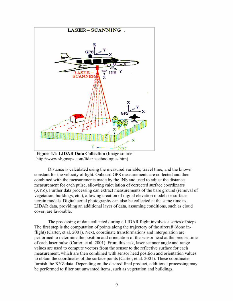
Experimental research work with LIDAR has been performed by researchers at the U.S. Department of Defense and NASA for a number of years; however the size, weight and power requirements of early LIDAR systems required them to be operated from large, four-engine aircrafts (Shrestha, et al. 2001). This made its widespread use difficult and expensive. With recent advances, LIDAR systems have reduced size, weight, and power requirements, while the accuracy of essential GPS systems has improved. Furthermore, advances in computer memory and processing speeds now allow the vast quantities of data collected by LIDAR to be stored and processed more quickly and efficiently. 4.4.1 Description of Technology The manner in which LIDAR works is fairly straightforward. A platform (usually an airplane) has a laser ranging system mounted onboard, along with other equipment including a precision GPS receiver and accurate Inertial Navigation System (INS) to orient the platform (Shrestha, et al. 1999). The platform is flown over the area in which data are to be collected, and the laser scans the area. The lasers utilized in this process typically emit thousands of pulses (up to 25,000) per second while in use. The travel time of these pulses is timed and recorded between the platform, the ground, and the platform once again (round trip), along with the position and orientation of the platform to determine range (distance) (Shrestha, et al. 2001). Figure 4.1 illustrates this process.

9

Figure 4.1: LIDAR Data Collection (Image source: http://www.sbgmaps.com/lidar_technologies.htm)

Distance is calculated using the measured variable, travel time, and the known

constant for the velocity of light. Onboard GPS measurements are collected and then combined with the measurements made by the INS and used to adjust the distance measurement for each pulse, allowing calculation of corrected surface coordinates (XYZ). Further data processing can extract measurements of the bare ground (removal of vegetation, buildings, etc.), allowing creation of digital elevation models or surface terrain models. Digital aerial photography can also be collected at the same time as LIDAR data, providing an additional layer of data, assuming conditions, such as cloud cover, are favorable.

The processing of data collected during a LIDAR flight involves a series of steps. The first step is the computation of points along the trajectory of the aircraft (done in-flight) (Carter, et al. 2001). Next, coordinate transformations and interpolation are performed to determine the position and orientation of the sensor head at the precise time of each laser pulse (Carter, et al. 2001). From this task, laser scanner angle and range values are used to compute vectors from the sensor to the reflective surface for each measurement, which are then combined with sensor head position and orientation values to obtain the coordinates of the surface points (Carter, et al. 2001). These coordinates furnish the XYZ data. Depending on the desired final product, additional processing may be performed to filter out unwanted items, such as vegetation and buildings.

10

The characteristics of flights performed to collect LIDAR data vary depending on

the project. Even the platform itself can vary; some laser scanners are mounted to helicopters while other scanners are mounted in airplanes. The determination of what platform will be used for collecting laser data often depends upon the project itself, as well as the capabilities of the organization chosen to perform the collection.

One of the primary uses of LIDAR data is in the creation of digital models of the earth’s surface. Traditional methods for producing such models (photogrammetry, field survey) are very time-consuming and therefore costly, especially in areas with dense vegetation, and often additional measurements are required later (Petzold, Reiss, and Stossel 1999). Through the use of filtering techniques, vegetation can be removed from LIDAR data, producing suitable results even in areas with dense vegetation. One study found that the accuracy of LIDAR derived models was equal or better to those produced by traditional photogrammetry (Petzold, Reiss, and Stossel 1999). 4.4.2 LIDAR Errors Research conducted by Huising and Piereira (1998) classified LIDAR errors into broad groups including laser, GPS/INS, and filtering induced, as well as errors caused by other problems. Laser induced errors stem from changes in height for the points on the terrain surface at a narrow angle (ridges and ditches), and grain noise, which can make smooth surfaces (beaches) appear rough. GPS/INS errors stem from equipment initialization errors and variances in the measurements taken by the instruments. Filtering errors stem from the incomplete and/or unnecessary removal of features, which may or may not be desired in the final dataset (vegetation, buildings, rock outcroppings). Other causes of error can stem from incomplete coverage of the survey area from improper flying and water bodies reflecting beams instead of absorbing them, producing a false reading. (Huising and Pereira 1998) 4.4.3 Use of LIDAR in Transportation Applications Al-Turk and Uddin (1999) examined the combination of a LIDAR derived DTM and digital imagery for digital mapping of transportation infrastructure projects. The authors state that such applications include asset management, right-of-way alignment, terrain modeling, and other transportation applications. The application of remotely sensed digital data (both LIDAR and imagery) would accelerate data collection and processing efforts that are essential for full and timely implementation of GIS-based infrastructure asset management systems. In addition, such data could be loaded into terrain mapping or computer-aided design (CAD) software, allowing further applications to be developed. The horizontal accuracy of the laser data was calculated to be 1 meter (3 feet) and the vertical accuracy was better than 7 centimeters (2.75 inches). (Al-Turk and Uddin 1999)

In a similar application, Pottle (1998) discusses the combination of LIDAR and video imagery to asset management for the capture of terrain and asset position information along busy rail corridors. The data were used to locate features such as mileposts, track centerlines, road crossings, switches, bridges, electrification, and culverts

11

for mapping purposes and DTM development. The data allowed engineers to analyze drainage conditions, measure distances between rails and clearances between overhead power lines, and model areas along the surveyed corridor. (Pottle 1998) Highway Mapping

Research conducted at the University of Florida evaluated the use of LIDAR derived terrain data for highway mapping. A thirteen-mile test flight was conducted over Interstate Highway I-10 in Leon County, Florida. Ground returns were processed to produce shaded relief maps, among other products. Roadway details revealed included an overpass, the directional lanes of the divided highway, the median divider, drainage ditches, and trees. In the unedited data, it was also possible to identify vehicles on the roadway. The horizontal resolution and positioning of the points were at the level of a few centimeters, so if profiles were taken along and across the highway, the grade and crown of the Interstate, along with the height of the overpass could be determined. (Shrestha, et al. 2000).

Additional research examined the accuracy of elevation measurements derived from laser data. This examination involved a comparison of heights derived from laser mapping and low altitude (helicopter-based) photogrammetry data collected in November 1997. Laser data were collected along a 50-kilometer (31-mile) corridor consisting of State Road 200 and Interstate Highway I-95 (Shrestha, et al. 1999). The elevations produced by laser data were found to be accurate to within ± 5 to10 centimeters (± 2–4 inches) (Shrestha, et al. 1999). The mean differences between photogrammetric and laser data were 2.1 to 6.9 centimeters (0.82 to 2.71 inches) with a standard deviation of 6 to 8 centimeters (2.36 to 3.15 inches) (Shrestha, et al. 1999). Railroad Lead-Track Route Location Cowen, et al. (2000) examined the inclusion of LIDAR data into an econometric model to determine the least cost path for a new railroad spur. A traditional field survey was also performed to assist in evaluating the accuracy of the LIDAR data (Cowen, et al. 2000). The data were examined to find the relationship between canopy closure, LIDAR canopy penetration and scan angle (Cowen, Jensen, and Hendrix, 2001). The research concluded that LIDAR appears to be a useful method to obtain XYZ data, even during growing seasons, although completely closed canopies in forested areas led to lower DEM accuracies (Cowen, et al. 2000). Where canopy closures were 30 to 40 percent, LIDAR pulses reached the ground 80 to 90 percent of the time (Cowen, et al. 2000). However, in areas where canopy cover was 80 to 90 percent closed, only 10 to 40 percent of LIDAR pulses reached the ground (Cowen, et al. 2000). Road Planning and Design

Investigations into the application of LIDAR-derived DTMs have been conducted in both The Netherlands and Canada to determine their suitability in highway planning and design (Berg and Ferguson 2000, 2001a; Pereira and Janssen 1999). The traditional mapping method being used by the agencies involved was photogrammetry, supplemented by ground surveys. The research conducted in these cases examined the use of LIDAR as a means to speed up data collection and surface mapping. In each case,

12

the accuracy of the data was examined to determine if it compared to the accuracies of data currently derived by photogrammetric means.

Research conducted in The Netherlands examined not only the applicability of laser data in highway planning and design, but also the additional information (both semantic and geometric) could be extracted (Pereira and Janssen 1999). This work was comprised of the detection, identification, modeling, measuring and labeling of such information (Pereira and Janssen 1999). The extraction research performed by the researchers focused extensively on the identification of breaklines, an important component in the planning and design process.

To assess the accuracy of the data, three additional sets of reference measurements were collected: two tachymetric (ground survey) datasets and one photogrammetrically derived dataset (derived from imagery collected in March 1996) (Pereira and Janssen 1999). For existing planning and design applications, a height accuracy of 25 centimeters (9.85 inches) was required. Accuracy of 7.5 centimeters (3 inches) was required for hard surfaces such as roads (Pereira and Janssen 1999). Assessment of the laser data found that its height (Z) accuracy was 29 centimeters (11.4 inches) root mean square error (RMSE). The accuracies obtained from tachymetry and photogrammetry (in soil with low grass) were 16 centimeters (6.3 inches) and 15 centimeters (5.9 inches), respectively. Laser data provided similar accuracies in similar areas; however, the RMSE of the laser data was affected by high inaccuracies in areas containing features such as ditches and slopes. This suggests that further research is required to address the shortcomings of LIDAR in these measurements.

The Ministry of Transportation Ontario (MTO) in Canada also conducted research into the application of LIDAR data in the highway planning and design process. The focus of this research was to determine if LIDAR data compared to data derived from photogrammetric mapping techniques and whether it would perform better than photogrammetry when leaves and ground vegetation were present (Berg and Ferguson 2001a). In order to make this determination, an examination of the horizontal and vertical accuracies of LIDAR was performed to see if they met the MTO specifications of 15 centimeters (5.9 inches) for hard surfaces and 20 centimeters (7.87 inches) for soft surfaces (Berg and Ferguson 2001a). To perform this analysis, data were collected during the summer under leaf-on conditions.

Analysis revealed that LIDAR data had an accuracy of 15 centimeters or better on hard surfaces, such as pavement (Berg and Ferguson 2000). The accuracies on other surfaces were variable up to 0.5 meters, while low vegetation, rocks, and ditches led to discrepancies of over one meter in some cases (Berg and Ferguson 2001a ). Under forested canopy, the accuracy of LIDAR data ranged from 0.3 meters to one meter (Berg and Ferguson 2000, 2001a ). LIDAR data were compared to MTO audit (ground surveyed) data, and no direct comparison was made to photogrammetric data produced under leaf-off conditions.

13

The MTO project presented a number of issues pertaining to the use of LIDAR data in highway planning and design. Most notably, difficulties were encountered with the ability of LIDAR to hit and define narrow features, such as ditches (Berg and Ferguson 2001a). This is particularly significant since the identification of such features is critical to define breaklines. The researchers also found that LIDAR was unable to penetrate low ground vegetation (Berg and Ferguson 2000). Comparisons to MTO audits reveled a number of discrepancies of up to 0.5 meters in areas covered with tall grass (Berg and Ferguson 2001). Rock cuts caused another point of concern. During the classification process, such features were assumed to be buildings by the software and automatically extracted (Berg and Ferguson 2001). Since rock features are an important factor in determining highways construction costs, they must be properly identified (Berg and Ferguson 2000).

14

5. STATE DOT LOCATION PROCESSES ` To better understand how remote sensing is used in highway location and design,

the location process for several states was documented. The location process of the Iowa DOT is presented first, along with a detailed description of how alignment alternatives are created. Documentation of the location process for Virginia and New Mexico is presented as well. 5.1 Iowa Location Process

The purpose of the location process in Iowa is to develop alternatives that are the most feasible from an engineering, environmental, and financial standpoint. Finding the best alignment within these constraints allows a project to be completed in a shorter timeframe than if projects are delayed due to concerns that are raised after the project commences. This timeframe for completion may be reduced from a maximum of 11 years to as few as six years, depending on the project. The following sections outline and provide a basic overview of the steps of the location process followed by the Iowa DOT (Iowa Department of Transportation 2001). 5.1.1 Receipt of Project Assignment

Potential projects are examined by decision makers and ranked to assign a priority to them. This ranking defines which projects are priorities and allows efforts to be focused on those priority projects that are likely to be funded. Projects that are authorized are programmed into the five-year program. 5.1.2 Project Management Team

A Project Management Team (PMT) is created for any size project expected to require an environmental document. Major projects involve the construction of a new alignment or realignment along a major portion of an existing highway. Minor projects generally use existing locations and usually involve the addition of lanes to a highway.

The PMT provides guidance and continuity to a project as it passes through all

phases, from planning to design to construction. The main responsibilities of the team are to set and maintain an on-time and on-budget project, as well as to identify and schedule necessary project resources. The PMT is coordinated by district staff and is lead by the district engineer. It is the responsibility of the engineer to create the PMT by selecting personnel from the Iowa DOT Offices of Corridor Development, Design, Environmental Services, Right of Way and the Federal Highway Administration (FHWA). Any additional expertise required from other offices may as necessary.

In a broad sense, the Transportation Commission defines the scope of a project in its five-year plans. This includes the determination of what type of facility the end result will be (2-lane, 4-lane, etc.) as well as its access control priority. However, more project-specific guidance is provided by the PMT.

15

5.1.3 Highway Location Process Once a project has been programmed, a number of project steps occur that take

the project from programming to final design. They include the following.

1) Development of Preliminary Route: This phase defines project corridors and location alternatives that meet the purpose and needs of the project. All areas where viable corridors or potential alignments may be located are identified during this step. Areas must be identified in enough detail for use in ordering aerial photography and DTM. Preliminary horizontal and vertical alignments, as well as access control scenarios are developed in this phase using existing aerial photography and quad maps. Environmental reviews for the identified corridors are also initiated. 2) Development of Route Alignments: A number of data elements are utilized to develop alternative alignments including terrain, engineering, property, and environmental information. This information is used to determine multiple alignment alternatives that will be considered by decision makers. Of particular importance to this research is the use of terrain data in the location process. As a general rule, the Iowa DOT attempts to produce alignments that meet three general criteria: engineering, environmental, and financial. In an engineering context, an alignment must be able to be realistically constructed with no formidable obstacles. Additionally, the project must not have a significant negative impact on the natural or human environment. An alignment should seek to avoid or minimize disruption to environmentally sensitive areas. Financially, a project must be feasible. While a project may be realistic and meet environmental constraints, if it is too costly to build, it is not a viable alternative. Alignments that meet these three criteria are considered viable alternatives. 3) Constraint Mapping: In this step, preliminary, existing data pertaining to the project area are gathered to determine locations that are suitable for locating alignments. Data include as-built plans, existing aerial photography, and topographic maps. These data are developed into constraint maps, which display areas that may be more or less suitable for locating alignment alternatives. Additional information is gathered from site surveys. Constraint mapping allows the study corridor area to be narrowed down. This gives designers a better idea of which areas within the entire project scope are viable and may require additional data such as aerial photography. Reducing the extent of the area for which data must be gathered saves time and reduces costs. 4) Creation of Alternative Alignments: When planning new alignments, designers examine existing roadway alignments to determine how much, if any can be saved and incorporated into alignment alternative. It is cost feasible to utilize portions of existing facilities wherever possible. Financial savings are derived from reduced engineering requirements for planning and design, property acquisition, and construction costs. The main consideration in the location of alignment alternatives is minimal disruption to private property. Essentially, the designer begins developing alternatives by laying out tangents that avoid passing through the middle of areas such as farm fields. When laying out an alignment, a designer seeks to follow property lines rather than transect property.

16

This creates less conflict with property owners and can reduce problems during Right of Way (ROW) acquisition.

Public input is also sought and considered when examining areas through which

alignments may be located. This input allows designers to understand property owner’s concerns. It also allows the opportunity for disputes to be settled during the early stages of development. Another area considered by designers is accessibility, which refers to how existing properties will access the new alignment. Properties must remain accessible to owners, but at the same time, access from the new facility is often controlled to some extent. Most often, for a specific project, access point locations (e.g. driveways) are to be spaced a specified distance apart.

The function of a facility after its construction is another concern. An alignment

that will be more costly to maintain is an alternative that is not as attractive as one with minimal maintenance costs. Terrain is relevant when determining alignment; alignments through more rugged terrain require more extensive maintenance than those traversing more level areas.

Once designers have a rough idea of where an alignment will be located, based on

the other considerations listed previously, they begin to consider terrain. Whenever possible, level terrain is followed for an alignment, while rugged terrain is avoided if possible. If there are no other alternatives to locate an alignment, then cuts and fills will be employed. In this case, the goal is to balance cut and fill locations to minimize the amount of borrow required for a project. Care must be taken when utilizing cuts and fills to prevent adverse affects from occurring in areas outside the project boundaries. For example, fill used for the approaches to a river crossing could result in flooding in another location downstream.

5) Selection of Most Feasible Alignments

A number of alternative alignments may be created for a project. However, it is impractical to present a large number of alternatives to the Transportation Commission for comparison and consideration. Consequently, the corridor development section meets as a group and narrows down the number of alternatives. Using past experience and engineering judgment, the corridor development section eliminates less attractive alternatives. A number of factors may limit an alternative’s attractiveness including property acquisition issues. The most feasible alternatives are selected and presented to the commission.

6) Collection of Project/Engineering Data

Once the final alignment alternative is selected, information for that alternative is gathered from various Iowa DOT offices to create a database. Any available data that are relevant, such as existing ROW, property ownership, addresses, businesses, preliminary property plats, and additional information, are gathered for the corridor being studied. Since, this data may not be complete, each office within the Iowa DOT is responsible for adding information and making changes as necessary.

17

Engineering data is also gathered during this phase such as accident history, pavement history, as-built plans, previous location and economic studies, sufficiency ratings, property information, utilities data, critical existing features, planned construction in adjacent areas, bridge and culvert information, and lifecycle cost analysis of existing pavement. This information is used to further identify corridor and location alternatives. All of these data are used to meet both internal and external project needs. Most importantly, by coordinating data, offices can prevent repetition in data collection. During this phase aerial photography and DTMs are ordered from the photogrammetry office, and traffic estimates are ordered from the systems planning office. 7) Public Information Meetings

Many meetings occur throughout the development process. Early public information meetings are held to inform the public of possible highway improvements. Public input concerning the project’s purpose, perceived transportation needs, and problem/issue identification in the project corridor(s) is gathered at these meetings. The result of this interaction is increased public awareness of and participation in the development process. 8) Environmental Data Gathering

During this phase, environmental studies are ordered from specialists for a corridor 400 meters on either side of the centerline for each alternative under consideration. These data are used to determine if there are any environmental concerns that could influence alignment alternatives, as well as what the acceptability of alternatives being proposed for study. Data collected for environmental review include regulated substances, cultural resources, historical and architectural sites, archeological sites, geotechnical information, biological information, and water resource/floodplain information. 9) Develop Alternatives

For all major and some minor projects, the corridor development section refines some of the alternatives identified during the development of preliminary route concept phase. Engineering and environmental data base maps are used to compare impacts for all alternatives. The main purpose of this phase is to transfer project concepts to an electronic layout for transfer to the design phase using CADD. Electronic outputs include horizontal and vertical alignments, typical cross sections, approximate construction need lines, intersection and interchange locations, planning level cost estimates, ROW impacts, and preliminary predetermined access (PDA) locations. This phase is intended to improve the identification of project impacts and respond to them during the planning phase. The result is a reduction in concept changes during the design phase of a project.

10) Public Involvement

Public involvement meetings are held to present project alternatives as well as their associated impacts. Information presented to the public at these meetings includes project concept, evaluation of impacts, anticipated entrance locations, alignment alternatives displayed in CADD layouts or over aerial photography, and environmental investigation results. The feedback received from the public at these meetings is used

18

(along with other factors) for evaluation, and ultimately definition of the preferred alignment.

11) Preparation of an Environmental Impact Statement

The environmental impact statement (EIS) provides a full and fair disclosure of all significant environmental impacts of a project. It also informs decision makers and the general public of the reasonable alternatives that avoid or minimize the adverse effects of a project while enhancing the quality of the human environment. An EIS serves as a means to assess the environmental impact of a proposed project; however, it cannot justify actions already taken. During this phase, preferred alternative alignments are identified, and reasonable alternatives are evaluated.

The final environmental impact statement documents compliance with all

applicable environmental laws and provides assurance that the requirements of these laws can be reasonably met. Mitigation measures to be incorporated into the project are also discussed in this document. Substantive comments received on the draft of the EIS and responses to those comments are also included, along with a summary of public input. 12) Combined Formal Public Hearing

A formal public hearing is intended to solicit public and agency comments on project alternatives and the anticipated social, economic and environmental impacts associated with each project alternative. Planning work for a project should be 100 percent complete by this phase, while design work should be near 30 percent complete. A transcript of the proceedings of this meeting is kept for future review by staff and the Transportation Commission as part of the project approval process. In addition to this transcript, staff prepares responses to the comments submitted at the hearing. 13) Commission Approval

A management level meeting is held to discuss a proposed project, its pros and cons, and stakeholder input. Out of these discussions, a preferred alignment alternative is selected for further development. This alignment is the one for which final design will proceed and construction will be pursued.

5.2 Virginia DOT Location Process

The Virginia Department of Transportation (VDOT) location process is designed to provide all parties with a significant interest in a project the opportunity to participate and influence the process. One of the benefits of this participation is the ability to reduce the adverse impacts of new facilities on property owners. In many alignment studies, environmental constraints (natural, historical resources) determine where an alignment will be located. This process facilitates early identification and analysis of such constraints. Figure 5.1 illustrates the VDOT highway location process. The location process consists of ten general steps, which are discussed in the following sections (Audit and Review Committee, 1998).

19

1) Early Project Notification Any project that will involve right-of-way acquisition, easements, or disturbance

of undeveloped land requires notification of state resource agencies. These agencies are given thirty days to provide VDOT with information concerning the project area. The goal of this early notification is to allow other agencies to identify adverse impacts that may occur as the result of a project. From this information, as well as site visits, preliminary environmental inventories of study areas are compiled. 2) Assignment of Work

Depending on whether the location study will be performed by VDOT or an outside consultant, a decision is made on whether subsequent work on the project will be conducted by district or central office staff. Most secondary location studies are conducted by district staff, while the remainder of location studies are performed by central office staff. Regardless of the entity performing the study, a study team is assigned to the project, in addition to a project manager. 3) Development of Purpose and Need

Early in the location process, a purpose and needs statement is drawn up to establish the justification for a project. If environmental impacts may occur with a project, it is the purpose and needs statement that validates the necessity of a project. The basis of the document is traffic data for the project area, identifying traffic problems or needs that will be met by the proposed highway project. Typically, such information includes travel demand, level of service, accident rates, and travel congestion. 4) Scoping and Data Collection

During this phase, VDOT begins to identify major issues of focus in the study area, as well as potential problems that may need to be addressed during the project. In addition, necessary data (aerial photography, traffic, environmental, right-of-way, cost) are collected. With this information, the DOT can better determine the potential location study areas where highway alternatives will be considered and developed. The photogrammetry data are also collected and produced during this phase. 5) Development of Potential Alternatives

The number of alignment alternatives developed varies considerably from project to project. When more significant impacts result, more alignment alternatives are created for a project. These alternatives may be produced by VDOT personnel, local governments, or even individual citizens. From the multiple alternatives developed, various combinations of route segments can be combined to produce the most favorable alternatives. Once preliminary alignments have been developed, a first stage of screening is performed to evaluate the different alternatives. This evaluation is based on

20

Figure 5.1: Flowchart of Virginia Highway Location Process (Source: http://jlarc.state.va.us/summary/rpt213/fig1.gif)

21

environmental and engineering factors, such as traffic, and is performed to eliminate alternatives that are not feasible, do not satisfy the purpose and need, or have severe impacts.

The alignment alternatives remaining after the first stage screening process,

undergo a second stage screening process. These alternatives are evaluated by criteria established by the project team including cost, public input, engineering feasibility, natural resource impact, community and public facility impact, etc. (Audit and Review Committee, 1998). With the criteria, alternatives are scored and ranked to provide a subset of alignments which will be carried forward for further analysis, specifically, environmental impact. 6) Design Development

Once preliminary alignments have been screened to provide viable alternatives, VDOT location and design staff become involved in the preliminary design of the remaining alternatives. Generally, these alternative alignments are designed to 10 percent to 15 percent of completion. This includes elements such as geometry, grade, quantities, and costs. This level of design allows project team members to accurately assess the impacts and costs of each alternative. 7) Public Information Meetings

At various stages of the location process, VDOT officials (and consultants if applicable) hold public meetings to provide general information on the project and to receive input and suggestions on alternatives. 8) Preparation of Draft Environmental Impact Statement

During this phase of the location process, an assessment is made of the environmental impacts of each alignment alternative. The impacts examined include land use, conservation, and air quality. The project team must analyze these impacts for each alignment. Critical impacts include traffic, land use, cultural resources, and water quality. 9) Submission for Public Comment and Location Hearing

Once a draft environmental impact statement has been created that meets FHWA approval, it is circulated to interested federal, state, and local agencies in the project for review and comment. In addition, a public hearing to consider public comment is held if there is interest for one. Such hearings provide a forum for VDOT to present alternatives and receive comments. 10) Staff Recommendation and Board Action

Once the period of public comment ends, VDOT staff reviews the information developed throughout the location process, as well as public comments. From this review, a recommendation for a preferred alignment is made. Typically, the administrator of the district in which the project is located makes the recommendation. It is then passed to the state location and design engineer, who in turn recommends it to the DOT’s chief engineer, who prepares a final recommendation for the Commonwealth Transportation

22

Board. The Commonwealth Transportation Board then makes a final decision on the selection of an alignment alternative (Virginia DOT, 2001).

5.3 New Mexico State Highway and Transportation Department Location Process

At the New Mexico State Highway and Transportation Department (NMSHTD), the location process is an interdisciplinary one. To select alignment alternatives, representatives from areas such as engineering, planning, and environmental participate. The goal of this multidisciplinary approach is to make informed decisions up front to meet both the project and the National Environmental Policy Act’s (NEPA) requirements. Figure 5.2 illustrates the New Mexico’s location process. The following sections provide an overview of the steps in their location process. 1) Scoping and Initiation

During this phase, the level of effort and general approaches that are appropriate for the particular study are identified. The level of effort determines what type of study should be conducted (corridor, alignment, etc.), a budget estimate, and the anticipated level of effort for the project to meet environmental clearance. Also, unique factors and issues are considered during this phase. These factors include drainage, mapping needs, environmental considerations, etc. Finally, a study team is put together during this phase. The study team is composed of a team leader, a district engineer, FHWA representatives, local representatives, and specialists (environmental, public involvement, utility, etc.). Project limits and study area are also defined. 2) Public Involvement

One of the policies of the NMSHTD is to begin any alignment or corridor study by developing and implementing a public involvement program. This program includes involving a number of diverse groups such as federal, state, and local agencies, potential users of the facility, property owners, and others who have a stake or interest in the project. Public involvement is sought through the entire location study. Through the public involvement plan, efforts are made to inform interested parties about proposed actions and attempt to involve these parties in the decision making process. In addition, input from these parties is sought to aid the study team in identifying issues and assist in evaluating the various alternatives. 3) Establish Purpose and Need

Defining the purpose and need of a project is one of the most important aspects of the location process. In New Mexico, the purpose is the overall objective to be achieved by the improvement. The need is a detailed explanation of the specific transportation problem or deficiency that currently exists or will exist in the future. To establish the purpose and need, various types of information are required. This information includes a description of the existing transportation system, the physical condition of the existing facility, an analysis of land use and growth trends, an analysis of existing and future traffic conditions, and a safety analysis. By establishing a purpose and need, alternatives can be compared and evaluated.

Figure 5.2: New Mexico Highway Location Process (New Mexico State Highway and Transportation Department, 2000)

23

24

4) Establish Existing Conditions/Constraints Potentially negative conditions are identified using existing data sources and field

reviews in order to avoid negative impacts to cultural, social and environmental resources and meet engineering constraints. In New Mexico, existing conditions are assessed in two steps: 1) inventory features in the study area, and 2) evaluate these features to determine how they might limit the location of a facility. 5) Identify Potential Alternatives

The fifth phase of the NMSHTD’s location process is identification of alignment alternatives. Alternatives are specific transportation improvement options that could be used to satisfy project needs. For smaller and/or rural projects, these alternatives might be different cross sections and alignments. In larger urban areas, alternatives might include non-highway options (transit, travel demand management, etc.). The goal of the study team is to develop alternatives that are in balance with the communities that they will serve and integrated into the surrounding environment. When developing alternatives, elements such as cultural and sensitive environmental features are avoided, as well as adverse terrain and other physical features that would require costly engineering solutions. It is important to note that the NMSHTD’s documentation states that precise terrain mapping is not required in this phase, but rather, only when the project moves into the final design phase. 6) Preliminary Evaluation of Alternatives

Once potential alternatives have been identified, an evaluation is made to narrow the list, which will be carried into the detailed evaluation phase. Evaluations are made using information gathered during previous phases of the process. The evaluations are made by qualified engineers, planners, and environmental specialists. Evaluation criteria are developed by the study team and are unique to each project. Once evaluations are completed, alternatives are compared, and less desirable or feasible alternatives are dismissed. 7) Detailed Engineering and Environmental Evaluation/Final Alignment Selection

The next step is a detailed evaluation of alternatives from both an engineering and environmental standpoint. This requires conceptual design plans produced earlier in the location process to be refined to an adequate detail to determine right-of-way requirements, costs, and impacts. These plans are developed from photo-based mapping to produce a plan and profile of each alternative. Information developed concerning right-of-way requirements, costs, and impacts are then analyzed and documented to compare the advantages and disadvantages of each alternative. Findings are presented at public meetings to update interested parties of the findings of the detailed studies conducted, as well as to receive feedback and answer questions those parties might have. Once environmental documentation and processing is completed, a preferred alignment is selected, and this selection moves to final design. (New Mexico State Highway and Transportation Department, 2000).

25

6. EVALUATION OF ACCURACY One of the main objectives of the research was to determine whether LIDAR data

were of sufficient accuracy for use in highway location studies. Originally it was thought that LIDAR could actually take the place of photogrammetry in producing surface terrain models for the various stages in highway location and design. However, as the research progressed, it became apparent that the currently available LIDAR product was not of sufficient accuracy for final design, even before accuracy studies were completed. However, since data can be collected more quickly, under more adverse conditions, and more cheaply with LIDAR than photogrammetry, it became apparent that the utility of LIDAR in the process would be in the preliminary design stages. Consequently, the objective of the accuracy comparison focused on accuracy adequacy for preliminary design compared to photogrammetry and to evaluate how well LIDAR performed under adverse conditions. In order to evaluate the elevation accuracy of LIDAR, a pilot study was conducted as described in the following sections. 6.1 Other Accuracy Studies

The majority of commercial organizations that collect LIDAR data, state that the vertical accuracy of their data is generally on the order of 15 centimeters (Sapeta 2001). However, a number of studies have examined the vertical accuracy of LIDAR data with varying results. Most of the studies reported on LIDAR data that were collected under leaf-off conditions (Pereira and Janssen 1999; Shrestha et al. 1999; Shrestha et al. 2001; Huising and Pereira 1998; Pereira and Wicherson 1999; Wolf, Eadie, and Kyzer 2000). Past research has also examined the accuracy of LIDAR data collected under leaf-on conditions (Berg and Ferguson 2000; Berg and Ferguson 2001b). Table 6.1 summarizes the results of other research. The variations in the accuracies achieved by these studies can be attributed, in part, to the differences between laser systems employed, flight characteristics, and the terrain being surveyed. As shown accuracy ranged from 3 to 100 centimeters, with the majority of the studies reporting from 7 to 22 centimeters. Table 6.1: Comparison of LIDAR Accuracy Application Vegetation Vertical Accuracy (cm) (RMSE) Road Planning (Pereira and Janssen 1998)

Leaf-Off 8 to 15 (flat terrain) 25 to 38 (sloped terrain)

Highway Mapping (Shrestha et al., 2001)

Leaf-Off 6 to 10 (roadway)

Coastal, River Management (Huising and Pereira 1998)

Leaf-Off 18 to 22 (beaches) 40 to 61 (sand dunes) 7 (flat and sloped terrain, low grass)

Flood Zone Management (Pereira and Wicherson 1999)

Leaf-Off 7 to 14 (Flat areas)

Archeological Mapping (Wolf, Eadie, and Kyzer 2000)

Leaf-Off 8 to 22 (Prairie grassland)

Highway Engineering (Berg and Ferguson 2000)

Leaf-On 3 to 100 (Flat grass areas, ditches, rock cuts) * Direct comparison to GPS derived DTM

26

6.2 Description of Study Area

A study corridor was selected to evaluate the accuracy of LIDAR derived terrain information compared to data derived from photogrammetry. The corridor was selected from existing DOT projects that already had surface elevation data available from photogrammetry. It was also critical that the photogrammetry work be fairly recent and that no significant changes had occurred within the study area from the time the photogrammetry data were completed. The Iowa Highway 1 (Iowa-1) corridor through Solon, Iowa, met all the requirements and was selected for a pilot study.

Iowa-1 is a two-lane, undivided state highway oriented north-south located in the

east-central portion of the state. The corridor is approximately 18 miles long. Photogrammetric data were available from the Iowa DOT for a 10-square-mile area around the corridor. The study segment begins at an interchange with Interstate 80 near Iowa City and ends at the junction with U.S Highway 30 outside the town of Mount Vernon. The highway passes through the town of Solon, the location of a proposed bypass, at about the midpoint of the corridor as shown in Figure 5.1. The corridor is characterized by a variety of terrain. The southern portion of the route passes through rolling farmland. At the midpoint of the study segment, the highway passes directly through the town of Solon. A few miles to the north of Solon, Iowa-1 crosses the Cedar River, with significant changes in elevation. 6.3 Photogrammetry The Iowa DOT Office of Photogrammetry provided digital elevation models developed by photogrammetric methods and the corresponding aerial photography in a digital format for the study corridor. These data were derived from a flight made on April 22, 1999. Photogrammetric data served as a “control” datasets for the accuracy comparison. The DTM generated for the Iowa-1 corridor was produced from aerial photography collected at an altitude of 2,000 feet. The compilation of breaklines and masspoints at an approximate spacing of 25 meters from these data was specified by the Iowa DOT Office of Photogrammetry in the project contract. It should be noted that this spacing was dependant on terrain, and a closer spacing was required in some areas to adequately represent the surface. Breaklines were defined to include roadway edge of shoulder, tops of banks, edges of water, toe/top of slope, and the tops of ridges. DTM data were compiled for a minimum distance of 150 meters on each side of the mainline (roadway) and sideroad centerlines of the proposed improvements, or to a specified distance. The Iowa DOT Office of Photogrammetry provided the following items for use in this research:

• Digital orthophotos • Breaklines and masspoints • Planimetric features • One-meter contours

All data were projected in the Iowa State Plane South coordinate system. The horizontal datum was NAD83, and the vertical datum was NAVD88, with units in meters. The geoid model was GEOID96.

27

Figure 6.1: Iowa-1 Corridor 6.4 Collection of LIDAR Data LIDAR data were also collected for the study corridor. LIDAR data were collected in October 2002. The vendor provided LIDAR-derived digital elevation data in the form of a point cloud consisting of an easting, a northing, and an elevation (XYZ) with an average spacing of 2 meters. Three datasets were provided: first return pulses, last return pulses, and bare earth. To produce a bare earth DEM, last return LIDAR pulses were processed with vegetation filters. Later work by the vendor produced a gridded DEM of 5 feet. All DEM data were delivered in comma delimited ASCII format. The laser unit utilized by the vendor sent out 4,000 pulses per second and scanned across the aircraft’s flight path. Additionally, GPS and inertial measurement unit (IMU) data were collected to record the aircraft’s position, as well as its roll, pitch and yaw at the time each pulse was fired by the laser. Digital orthophotos were also collected during a separate flight from the LIDAR data collection. Digital images were of one-foot resolution, with a horizontal accuracy of two meters. Imagery was orthorectified using airborne GPS data, platform attitude, and LIDAR DEM data. All data were projected in the Iowa State Plane South coordinate system. The horizontal datum was NAD83, and the vertical datum was NAVD88, with units in meters. Because LIDAR was flown in the late fall, significant vegetation was still present. Harvesting of corn and soybeans, the two crops present in fields adjacent to Iowa-1, had

28

commenced. As a result, some fields were harvested and others were not. This provided the unique opportunity to compare data for both leaf-on and leaf-off conditions. 6.4 GPS Data

Since the study area was an existing DOT relocation project, a complete photogrammetry product was available for the entire study area. The Iowa DOT currently uses photogrammetry data for the entire highway location process, including final design, so it was felt that the photogrammetry dataset would provide a good baseline for comparison of LIDAR elevation information.

It was also decided that high accuracy GPS data would be collected and used to

compare both the LIDAR and photogrammetry for a limited subset of the corridor. In April 2002, a consultant was hired to collect 177 GPS points at various locations throughout the study corridor to validate the accuracy of both the LIDAR and photogrammetry datasets. All data were projected in the Iowa State Plane South coordinate system, NAD83, NAVD88, and GEOID96. The GPS points were collected with a Trimble GPS. The stated horizontal accuracy of the equipment was 10mm + 1ppm and the vertical accuracy was 20mm + 2ppm. 6.5 Accuracy Comparison Methodology

A number of different methodologies are available to compare accuracy between two elevation datasets. Each of these methods has their own advantages, as well as limitations. The following sections provide an overview of these techniques. 6.5.1 Direct Point Comparison

Shrestha, Carter, Lee, Finer, and Sartori discuss a direct point comparison that used a base reference dataset with elevations. A computer program was used that extracts points from a LIDAR dataset that are within a user specified tolerance (both x and y, as well as z) of the base reference points (e.g. within one meter horizontal and 25 centimeter vertical). A computer program was used to extract LIDAR points that were within the specified tolerance. Elevational differences between the reference and LIDAR points were used to calculate accuracy statistics. The main advantage is that exact points between the two datsets can be compared directly with this method. It also takes advantage of the probability that the dense nature of the distribution of LIDAR points will lead to a given number of those points lying in close proximity to reference points. The disadvantage of this method is that the researcher must specify the given tolerance (circumference) around reference points from which points being compared (e.g. LIDAR) can be extracted. The specification of different tolerances could lead to greater or fewer common points being identified, potentially producing different statistical results for vertical accuracy. 6.5.2 Point Interpolation

A number of studies performed accuracy comparisons by bilinearly interpolating LIDAR points to reference points (either photogrammetric or GPS) (Pereira and Janssen 1999; Huising and Pereira 1998; Pereira and Wicherson 1999; Wolf, Eadie, and Kyzer 2000). To minimize interpolation error, only points on flat surfaces, such as roads, are

29

used. The difference between the reference point and the interpolated LIDAR point is then determined to calculate appropriate statistics such as the root mean square error.

The advantage of this method is that direct point comparisons can still be made, but the reference points and LIDAR datapoints do not have to be within a specified tolerance of each other. The disadvantage of this method is that only interpolated points from flat areas are used for comparison to take advantage of linearity and minimize error. This prevents a determination of the vertical accuracy of LIDAR on non-flat areas, such as sloped terrain. 6.5.3 Grid Comparison In modeling surfaces terrain, the elevational accuracy of the entire surface is important, not just elevations on hard, flat surfaces. To eliminate the assumption of linearity associated with point interpolation, nonlinear interpolations methods, such as inverse distance weighting (IDW) and splines, can be used for accuracy comparisons. Nonlinear interpolation methods assume that the closer points are to one another, the more likely they will affect one another (DeMers 2000). When grids of the same resolution are produced for both the control and test dataset, it is possible to perform a comparison of the elevation between datasets for any location throughout a study area by comparing grid cell values.

The advantage of using grids to determine accuracy is that they represent the entire surface of the area being examined. This allows for comparisons to be made on a number of different surfaces of interest (roads, ditches, etc.). The disadvantage of this method is that more sparsely populated datasets, such as photogrammetry that do not contain the same large number of points as LIDAR, may produce a less accurate representation of the earth’s surface as grid resolution is increased. In addition, when dealing with datasets, such as LIDAR, that contain millions of individual points, grid production can be a time- and processor-intensive operation, even for the most advanced computers. 6.6 Surface Comparison Another method is to compare the accuracy elevations based on a comparison of surfaces (Triangulated Irregular Networks or TIN) generated from the control and test datasets. The TIN model generates a representation of the surface based on the relationship between neighboring points in a dataset. Unlike gridding, where mathematical processes fill in the gaps between points with interpolated points, triangulation connects neighboring points to create a surface model. To compare surface models, test points for which accuracy is to be determined are selected, with the elevations of the selected points either being extracted by a geographic information system (GIS) or manually recorded. The advantage of TIN comparison is that it is a less processor- and time-intensive procedure than grid comparison. In addition, automated extraction of elevational values for points of interest is possible within a GIS environment. A disadvantage to this method is that with less densified terrain models (e.g. photogrammetry), elevational changes

30

between triangulated points may not be represented, as a sudden drop in elevation for a ditch might not be sufficiently modeled by the TIN. The result would be an incorrect determination of the true elevational accuracy of the test dataset. Another disadvantage is that surface terrain models are based on mathematical computations, consequently, accuracy is affected by the algorithms used as well as the data itself 6.7 Statistical Test

The vertical accuracy of LIDAR data can be influenced by the type of laser system employed, the measurement process used, and the terrain itself (Pereira and Janssen 1999). It can also be influenced by the acquisition and processing strategy of the vendor (Pereira and Janssen, 1999). Filtering procedures can also have an effect on the vertical accuracies of LIDAR (Berg and Ferguson 2001).

The National Standards for Spatial Data Accuracy (NSSDA) specifies that the accuracy of a dataset is be determined by comparing the coordinates of several points in a test dataset with an independent data set of greater accuracy. For this research, LIDAR data were compared independently to two different datasets. First data were compared to data collected using photogrammetry as discussed previously. Next data were compared for a smaller area of the test study area to GPS points. The NSSDA recommends points found at right-angle intersections (roads, railroads, canals, etc.), as well as utility access covers and sidewalk and curb intersections be used for this evaluation (Minnesota Planning Land Management Information Center 1999). However, because LIDAR data are so dense and randomly distributed, identifying points that fall directly on such features was not possible. Instead, the grid comparison method was used to develop grids of various resolutions. Points in these grids were extracted and compared to one another to perform accuracy assessments. 6.7.1 National Standards for Spatial Data Accuracy The NSSDA outlines a statistical testing methodology for estimating the positional accuracy of digital geospatial data with respect to georeferenced ground positions of higher accuracy (FGDC, 1998). This test applies to any georeferenced digital geospatial data derived from sources such as aerial photographs, satellite imagery, and ground surveys. Twenty or more test points are required to conduct a statistically significant accuracy evaluation, regardless of the size of the data set or area of coverage (Minnesota Planning Land Management Information Center 1999). It also allows for the reasonable computation of a 95 percent confidence interval, meaning that, when 20 points are tested, it is acceptable that one point may exceed the computed accuracy (Minnesota Planning Land Management Information Center 1999). If fewer than 20 test points are available, three alternatives are available for determining positional accuracy: deductive estimates, internal evidence, or comparison to source (Minnesota Planning Land Management Information Center 1999).

To perform the accuracy comparison between LIDAR and photogrammetry, an adaptation of the recommended NSSDA methodology was utilized. The steps are as follows:

31

1. Determine what accuracy (horizontal, vertical, or both) is to be tested. In this research, only vertical accuracy was be tested.

2. Select an independent dataset of higher accuracy that corresponds to the data being tested. In this research, the first independent dataset was the photogrammetry data previously produced for the Iowa-1 corridor. The second independent dataset was the GPS dataset.

4. Select a common set of test points from each of the datasets being compared needs to be collected. The grid comparison method was used to select points. LIDAR was evaluated for different types of surfaces in the field (hard surface, fields, etc.).

5. Calculate the positional accuracy statistic using an RMSE test. 6.7.2 RMSE Test The test used to evaluate vertical accuracy was the root mean square error test. The RMSE test estimates the common within-group standard deviation of data. To compute the RMSE, twenty or more test points are required to conduct a statistically significant evaluation, regardless of the size of the dataset or area of coverage (Minnesota Planning Land Management Information Center 1999). The test statistic is of the form (Federal Geographic Data Committee 1998; Shortridge 2000; Minnesota Planning Land Management Information Center 1999):

RMSEz = ( )

nXX 2

i e,test valui value,ground ∑ −

Where i value,ground X : ground truth point of the ith point in the dataset i e,test valuX : test point of the ith point in the dataset

∑ ( )e test valu valueground XX − 2 : sum of the set of squared differences between the ground and test data

n : total number of test points

To determine the NSSDA accuracy statistic, the RMSE value derived from the above calculation is multiplied by a value that represents the mean at the 95 percent confidence level (Minnesota Planning Land Management Information Center 1999). For vertical accuracies, this value is 1.96. For horizontal accuracies, the value is 1.7308. The accuracy statistic is calculated with the following equation: NSSDA = Accuracyr = 1.96 * RMSEz 6.8 Results

Several comparisons were made to determine the accuracy of LIDAR as it compares to both photogrammetry, as well as GPS readings collected in the study area.

32

LIDAR accuracy was evaluated for several different types of terrain. Results of the accuracy analyses are presented in the following sections. 6.8.1 Using GPS as Control Points

The first accuracy test consisted of comparing LIDAR points to GPS points and then comparing photogrammetry derived points to GPS points for several surface types. Elevations for GPS control points were compared to elevations from grids of 1-, 5- and 10-meter resolution developed from both TINs and IDW interpolation. The following sections discuss the results of the accuracy comparisons performed using GPS as control. Hard Surfaces

It was expected that LIDAR would be the most accurate on hard surfaces such as asphalt or concrete roadway surfaces. Results are presented in Table 6.2. Both photogrammetry and LIDAR data produced mixed results. Photogrammetry elevations were more accurate than LIDAR for TIN-derived grids. However, LIDAR performed better than photogrammetry when IDW interpolation was used to produce a surface. As a whole, the accuracy of each dataset declined as grid resolution became coarser. This is to be expected, as a greater elevation generalization is made as the size of the grid cell expands to include more known elevational points. Overall, neither LIDAR nor photogrammetry elevations were found to be close in accuracy to GPS control on hard surfaced areas. Table 6.2: Accuracy of LIDAR and Photogrammetry Compared to GPS Control on Hard Surfaces Resolution Grid Dataset Sample

Points Mean Elevation

RMSE (meters)

NSSDA (meters)

PHOTOGRAMMETRY 66 0.03 0.17 0.32 TIN LIDAR 66 0.11 0.33 0.64 Photogrammetry 66 0.40 0.64 1.25

1-meter

IDW LIDAR 66 0.10 0.32 0.63 Photogrammetry 66 0.03 0.18 0.35 TIN LIDAR 66 0.13 0.36 0.70 Photogrammetry 66 0.36 0.60 1.18

5-meter

IDW LIDAR 66 0.16 0.40 0.78 Photogrammetry 66 0.11 0.33 0.65 TIN LIDAR 66 0.32 0.57 1.12 Photogrammetry 66 0.46 0.68 1.33

10-meter

IDW LIDAR 66 0.35 0.59 1.15

33

Ditches The results of the accuracy comparisons for ditches are presented in Table 6.3.

Neither LIDAR nor photogrammetrically derived grids performed well in ditch areas. While photogrammetry did produce more accurate elevations in ditch areas for TIN grids, this can mainly be attributed to the inclusion of breakline elevations, which defined such features when producing the terrain models. LIDAR elevations for ditch areas were quite poor. The lowest RMSE achieved, 0.60, does not even approach the 15-centimeter (0.15 meter) accuracy claimed by LIDAR vendors. As a whole, neither LIDAR nor photogrammetry elevations in ditch areas were found to be highly accurate at any resolution when compared to GPS control elevations. Table 6.3: Accuracy of LIDAR and Photogrammetry Compared to GPS Control on for Ditches Resolution Grid Dataset Sample

Points Mean Elevation

RMSE (meters)

NSSDA (meters)

Photogrammetry 25 0.27 0.52 1.02 TIN LIDAR 25 0.36 0.60 1.17 Photogrammetry 25 0.55 0.74 1.45

1-meter

IDW LIDAR 25 0.39 0.63 1.23 Photogrammetry 25 0.39 0.62 1.22 TIN LIDAR 25 0.52 0.72 1.41 Photogrammetry 25 0.68 0.82 1.62

5-meter

IDW LIDAR 25 0.46 0.68 1.33 Photogrammetry 25 0.60 0.77 1.52 TIN LIDAR 25 0.62 0.78 1.54 Photogrammetry 25 0.91 0.96 1.87

10-meter

IDW LIDAR 25 1.27 1.139 2.21

Slopes

Table 6.4 presents the results of accuracy evaluations performed on slopes. Both photogrammetry and LIDAR performed poorly for areas of steep slopes (e.g. near creeks, etc.). While photogrammetry did produce better results than LIDAR, this may be attributed to the inclusion of breakline data when developing the surface models. LIDAR performed especially poorly in sloped areas. This could be due to the potential for LIDAR to miss sections of slope where abrupt terrain changes occur, such as the true bottom of a slope. The result is an incorrect surface model being created and producing a large accuracy difference.

34

Table 6.4: Accuracy of LIDAR and Photogrammetry Compared to GPS Control on for Steep Slopes Resolution Grid Dataset Sample

Points Mean Elevation

RMSE (meters)

NSSDA (meters)

Photogrammetry 10 0.77 0.28 0.54 TIN LIDAR 10 0.26 0.51 1.00 Photogrammetry 10 0.09 0.31 0.60

1-meter

IDW LIDAR 10 0.19 0.43 0.84 Photogrammetry 10 0.05 0.22 0.43 TIN LIDAR 10 0.13 0.36 0.71 Photogrammetry 10 0.14 0.38 0.74

5-meter

IDW LIDAR 10 0.22 0.47 0.92 Photogrammetry 10 0.51 0.72 1.40 TIN LIDAR 10 0.70 0.84 1.64 Photogrammetry 10 0.26 0.51 1.01

10-meter

IDW LIDAR 10 0.64 0.80 1.57

Bare Surfaces

Results of vertical accuracy comparisons for bare surfaces, such as harvested fields, are presented in Table 6.5. Both datasets performed well on bare earth surfaces as would be expected. LIDAR results were similar for all resolution. Most of the RMSE were slightly outside the 15-centimeter stated accuracy. They were also comparable for both TIN and IDW. This suggests that LIDAR performs well when representing terrain for flat, bare surfaces. Photogrammetry performed well on bare surfaces as well. For the 1- and 5-meter resolution, the RMSE was around 10 centimeters. Row-Crop Vegetation A number of fields in the study area were unharvested when LIDAR was completed. Corn and soybeans are the predominant crop in the area. The data was collected in late fall when crops were fully-grown and would have presented a worst-case scenario. Photogrammetry was collected under leaf-off conditions so there was no comparison database. One of the main advantages of LIDAR is that it is able to penetrate vegetation so that data can be collected. The amount of vegetation that can be present before LIDAR becomes unreliable is unknown. However, under full leaf-on conditions with the relatively dense vegetative conditions that would have been present at the end of the growing season, LIDAR performed fairly poorly. As shown in Table 6.6, at all resolutions, the RMSE for LIDAR data were around 0.50 meters.

35

Table 6.5: Accuracy of LIDAR and Photogrammetry Compared to GPS Control on for Bare Surfaces Resolution Grid Dataset Sample

Points Mean Elevation

RMSE (meters)

NSSDA (meters)

Photogrammetry 25 0.01 0.09 0.18 TIN LIDAR 25 0.04 0.19 0.38 Photogrammetry 25 0.01 0.10 0.20

1-meter

IDW LIDAR 25 0.03 0.18 0.34 Photogrammetry 25 0.01 0.10 0.20 TIN LIDAR 25 0.04 0.21 0.40 Photogrammetry 25 0.01 0.12 0.23

5-meter

IDW LIDAR 25 0.04 0.20 0.39 Photogrammetry 25 0.02 0.13 0.26 TIN LIDAR 25 0.04 0.21 0.41 Photogrammetry 25 0.02 0.15 0.30

10-meter

IDW LIDAR 25 0.03 0.16 0.32

Table 6.6: Accuracy of LIDAR Compared to GPS Control on for Row-Crop Vegetation Resolution Grid Dataset Sample

Points Mean Elevation

RMSE (meters)

NSSDA (meters)

TIN LIDAR 23 0.21 0.46 0.90 1-meter IDW LIDAR 23 0.20 0.44 0.87 TIN LIDAR 23 0.21 0.465 0.89 5-meter IDW LIDAR 23 0.22 0.486 0.92 TIN LIDAR 23 0.21 0.46 0.90 10-meter IDW LIDAR 23 0.23 0.49 0.94

6.8.2 Using Photogrammetry as Control Points The vertical accuracy of LIDAR was also compared using the photogrammetric data as control points. This allowed the accuracy of LIDAR to be tested over larger areas since only a few GPS points were selected for each surface type. Using photogrammetry as the control, the accuracy of LIDAR in comparison to the Iowa DOT’s currently accepted data collection method could be evaluated. Hard Surfaces

The results of the accuracy comparisons performed on hard surfaces are presented in Table 6.7. On hard surfaces, the elevational accuracy of LIDAR is mixed. While LIDAR appears to produce fairly accurate elevations from TIN-derived grids, the same is not true for grids produced by IDW interpolation. None of the accuracies approached those required for DOT activities. However, it should be noted that the accuracy of

36

LIDAR under both grid types stayed fairly constant as grid resolutions declined. It should also be noted that for this analysis LIDAR is being compared to photogrammetry. As demonstrated in the previous sections, there are some inaccuracies in the photogrammetry data as well. Additionally most LIDAR accuracy comparisons presented in other studies used highly accurate control points such as GPS for comparison. In section 6.7.1, photogrammetry for the study corridor was compared to GPS control. For hard surfaces the accuracy was around 0.17 meters and for bare earth surfaces the accuracy was around 0.1 for the one-meter resolution grids. Table 6.7: Accuracy of LIDAR Compared to Photogrammetry Control for Hard Surfaces Resolution Grid Dataset Sample

Points Mean Elevation

RMSE (meters)

NSSDA (meters)

TIN LIDAR 140,176 0.07 0.27 0.531-meter IDW LIDAR 139,865 0.21 0.46 0.89TIN LIDAR 5,555 0.07 0.27 0.535-meter IDW LIDAR 5,560 0.20 0.45 0.88TIN LIDAR 1,375 0.08 0.28 0.5510-meter IDW LIDAR 1,379 0.21 0.45 0.89

Ditches

LIDAR data collected in areas where ditches were present were also compared to photogrammetry. As expected given previous results using GPS as the control points, LIDAR elevations in ditch areas were not accurate. This inaccuracy can be attributed to the lack of supplemental information, such as breaklines, which define features like ditches. Without such information, surface models developed exclusively from LIDAR data will only generalize the terrain for such areas, producing less accurate results. The results of accuracy comparisons performed for ditches are presented in Table 6.8. Table 6.8: Accuracy of LIDAR Compared to Photogrammetry Control for Ditches Resolution Grid Dataset Sample

Points Mean Elevation

RMSE (meters)

NSSDA (meters)

TIN LIDAR 144,995 0.17 0.41 0.811-meter IDW LIDAR 141,560 0.22 0.47 0.92TIN LIDAR 5,742 0.18 0.43 0.845-meter IDW LIDAR 5,729 0.21 0.46 0.90TIN LIDAR 726 0.13 0.36 0.7010-meter IDW LIDAR 1,426 0.31 0.55 1.09

Wooded Areas Table 6.9 presents the results of accuracy evaluations for LIDAR in wooded areas. In areas where trees were present, LIDAR once again produced mixed results. While the vendor did perform filtering to remove vegetation in such areas, the elevational

37

accuracies achieved still were not adequate. Interestingly, the elevational accuracy of surface models developed from TIN-derived grids was significantly better than those with IDW interpolation. One explanation for this may be that in order to remove vegetation or structures, LIDAR points are removed during filtering procedures and that interpolation overcompensates for the lack of elevational data. Table 6.9: Accuracy of LIDAR Compared to Photogrammetry Control for Wooded Areas Resolution Grid Dataset Sample

Points Mean Elevation

RMSE (meters)

NSSDA (meters)

TIN LIDAR 215,143 0.43 0.66 1.291-meter IDW LIDAR 143,335 1.22 1.11 2.17TIN LIDAR 8,614 0.42 1.15 2.255-meter IDW LIDAR 7,953 1.32 1.15 2.25TIN LIDAR 2,155 0.45 0.67 1.3210-meter IDW LIDAR 1,981 1.36 1.17 2.28

Bare Earth The accuracy of LIDAR data for bare earth surfaces such as harvested fields, produced results similar to those for hard surfaces as shown in Table 6.10. This suggests that LIDAR does perform favorable on bare, flat surfaces. The grids produced from TINs once again produced more accurate terrain models than those of IDW interpolation. Both grid types produced consistent results for each resolution, further suggesting that LIDAR is a more promising technology in flat areas. However, the accuracies achieved in harvested areas still are not close to those necessary for location and design activities, nor do they approach an RMSE of 15 centimeters. Table 6.10: Accuracy of LIDAR Compared to Photogrammetry Control for Wooded Areas Resolution Grid Dataset Sample

Points Mean Elevation

RMSE (meters)

NSSDA (meters)

TIN LIDAR 1334610 0.1027 0.3205 0.62811-meter IDW LIDAR 1685998 0.1929 0.4392 0.8608TIN LIDAR 67446 0.0855 0.2924 0.57315-meter IDW LIDAR 67445 0.1922 0.4384 0.8593TIN LIDAR 16806 0.0872 0.2953 0.578810-meter IDW LIDAR 16806 0.1891 0.4349 0.8523

Unharvested Fields (Low Vegetation) Table 6.11 presents the results of accuracy evaluations performed on unharvested fields with low vegetation, which included areas with crops such as soybeans that were

38

not harvested before LIDAR data collection occurred. Unharvested low vegetation fields produced accuracies close to those produced in harvested fields. This suggests that LIDAR may be capable of penetrating low, less dense vegetation, such as soybeans. As was found with accuracy evaluations for other areas, as grid resolution degraded, accuracy remained fairly constant. Table 6.11: Accuracy of LIDAR Compared to Photogrammetry Control for Unharvested Fields with Low Vegetation Resolution Grid Dataset Sample

Points Mean Elevation

RMSE (meters)

NSSDA (meters)

TIN LIDAR 1,320,236 0.12 0.35 0.691-meter IDW LIDAR 1,320,081 0.21 0.46 0.90TIN LIDAR 52,862 0.12 0.35 0.695-meter IDW LIDAR 52,862 0.21 0.46 0.90TIN LIDAR 13,250 0.21 0.46 0.9010-meter IDW LIDAR 13,250 0.12 0.35 0.69

Unharvested Fields (High Vegetation)

Table 6.12 presents the results of accuracy evaluations performed on unharvested fields with high vegetation. This type of surface included areas with corn that had not been harvested when LIDAR data were collected. LIDAR does not perform adequately under heavy vegetation, as evidenced by errors of over one meter (RMSE) calculated for terrain models regardless of resolution. This demonstrates that LIDAR pulses are not capable of penetrating dense foliage, such as corn, and returning a true elevation of the earth’s surface. While further filtering aids in the removal of such dense vegetation, the poor performance of LIDAR to initially penetrate crop canopy illustrates that such data collection might be more feasible under leaf-off conditions or when crops, such as corn, are in earlier stages of growth. Table 6.12: Accuracy of LIDAR Compared to Photogrammetry Control for Unharvested Fields with High Vegetation Resolution Grid Dataset Sample

Points Mean Elevation

RMSE (meters)

NSSDA (meters)

TIN LIDAR 2,670,799 2.19 1.48 2.901-meter IDW LIDAR 2,658,448 2.61 1.61 3.16TIN LIDAR 106,765 2.18 1.48 2.905-meter IDW LIDAR 106,819 2.62 1.62 3.17TIN LIDAR 26,737 2.19 1.48 2.9010-meter IDW LIDAR 26,759 2.65 1.63 3.19

39

6.9 Study Limitations An additional limitation of this research was that the photogrammetric and LIDAR data were produced at different times. Ideally, the LIDAR data and the aerial photography required for photogrammetric mapping would be collected on the same day and if possible the same flight. Instead, a two-year gap existed between photogrammetric mapping (1999) and LIDAR collection (2001). This gap allowed for changes to occur in the field; while significant terrain changes did not occur in the area, minor, less noticeable changes could have occurred. Such minor changes could lead to natural differences in elevation, subsequently affecting the results of accuracy comparisons. 6.10 Conclusions The primary conclusion drawn from the analysis presented here is that LIDAR elevation data collected under leaf-on conditions are not accurate enough to serve as a stand-alone terrain product for DOT highway planning and design functions. However, the higher accuracies achieved on clutter-free surfaces (harvested fields and hard surfaces) suggest that LIDAR data collected under conditions with lower vegetation conditions may produce better accuracy. Areas of significant terrain change (e.g. ditches) may still be misrepresented by LIDAR due to the potential for LIDAR points to miss significant portions of such areas, such as the bottom of the ditch. However, inclusions of breaklines may produce accurate terrain models with LIDAR. LIDAR data also failed to yield accurate results in areas of heavy vegetation, specifically wooded areas and unharvested fields containing high vegetation. This indicates that LIDAR is not capable of penetrating such dense vegetative coverage. LIDAR did perform better in areas of low vegetative cover, suggesting that light pulses may be capable of penetrating foliage that is less dense and closer to the earth’s surface. In areas of more dense vegetation, it appears that the pulses are not able to reach the ground and that LIDAR used under dense vegetation may provide readings that indicate the top of vegetation rather than the actual ground. Even with preliminary vegetation filters utilized by the vendor all vegetation was not removed from the bare earth model. Further vegetation filtering performed by the vendor did remove high vegetation, such as corn. This suggests that, while effective for dense vegetation, current filters are not capable of removing all varieties of foliage. Further refinements to such filters will be necessary before LIDAR is capable of producing accurate terrain models collected under leaf-on conditions. Although LIDAR elevational data are not accurate enough to replace photogrammetry in planning and design activities, such data can still be used in the location process. Section 7 presents a methodology for implementing LIDAR data collection into the highway location and design process.

40

7. OVERVIEW OF THE IOWA DOT EXPERIENCE WITH LIDAR FOR A HIGHWAY LOCATION STUDY

At the same time this research was going on, the Iowa DOT was also in the process of evaluating LIDAR in the highway location process for a different highway corridor. One of the research tasks was to document the Iowa experience with LIDAR. The process is still underway at the DOT, therefore only the initial data collection stages are documented.

Although Iowa DOT personnel have been aware of LIDAR technology for some

time, it wasn’t until recently that they felt that LIDAR technology had advanced to the point where it was feasible to collect terrain data for location and design projects. In the summer of 2001, LIDAR was used to collect position and elevation data for a relocation study along U.S. Highway 30 (U.S. 30). DOT personnel were interested in evaluating whether data collection with LIDAR could compliment traditional photogrammetric methods and expedite the design process. Currently, the Iowa DOT uses soft-copy photogrammetry for large-scale location studies. As discussed, collection of aerial imagery is limited to optimal environmental conditions, and data reduction takes a significant amount of time in the office once imagery is acquired. As a result, time requirements for large corridor studies are prohibitive especially if optimum windows for collection of imagery are missed. For example, if resources cannot be mobilized to take aerial photographs in the spring before significant vegetation is present, collection of imagery may be pushed back until late fall, delaying other project activities that rely on imagery and terrain information.

Due to current accuracy constraints, LIDAR is expected to supplement rather than

replace traditional photogrammetry. The ability to begin initial location and environmental studies significantly in advance of current timelines is the value that LIDAR could add to location studies. LIDAR data would be used to evaluate initial alternatives and narrow down the corridor areas down to those for the final alignment, reducing the amount of higher accuracy photogrammetry that has to be performed. LIDAR data collection is expected to be significantly faster and less costly than photogrammetry would be for a large study area. 7.1 Project Description

To test the feasibility of using LIDAR data in location and design studies, LIDAR was flown for an upcoming relocation project at the DOT that consisted of a 46-mile corridor of U.S. 30 from the town of Lisbon, in Linn County, to DeWitt, in Clinton County. The corridor is displayed in Figure 7.1. Project plans include adding additional lanes, roadway realignment in some locations, and the construction of seven bypasses throughout the corridor. The LIDAR data were collected to provide general terrain information, with the plan to collect more detailed information from aerial photography using photogrammetry for final design.

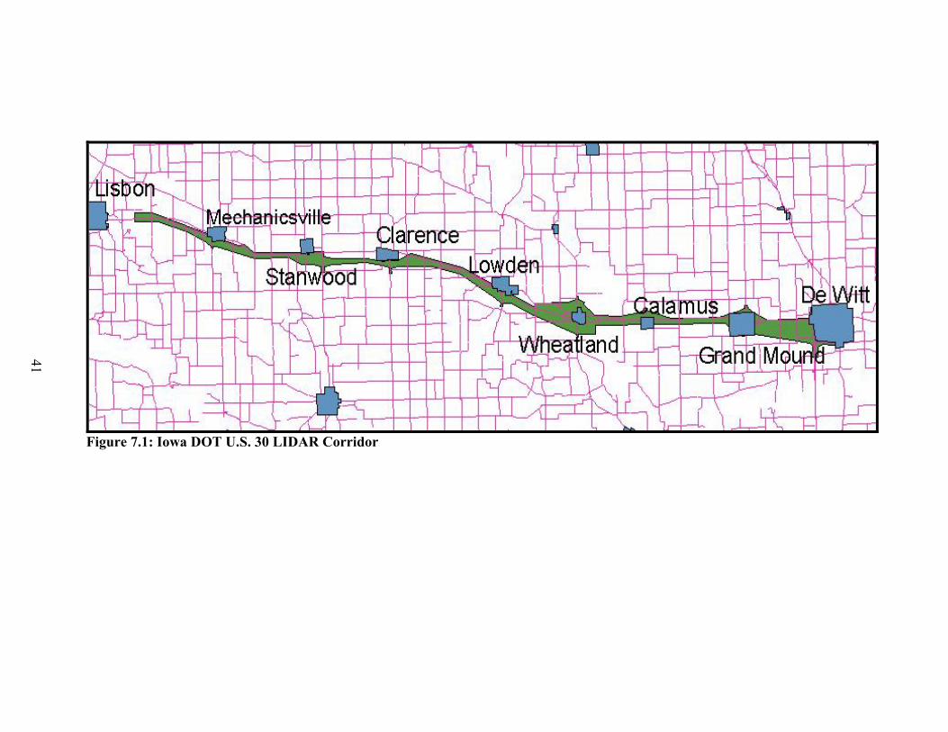
Figure 7.1: Iowa DOT U.S. 30 LIDAR Corridor

41

42

7.2 LIDAR Data Collection The Iowa DOT solicited proposals for LIDAR data collection and originally

intended to receive all proposals from perspective consultants by December 21, 2000. Final selection of the consultant was scheduled for January 2001. According to this timetable, completion of contracts would occur by March 2001, and the resulting flights would take place shortly thereafter, under leaf-off conditions. Delivery of the final product was expected by June 1, 2001, according to original timetable. For various reasons, many of these dates were not met. However, none of the missed deadlines were detrimental to the project. 7.2.1 Consultant Selection A preliminary search of consultants was made to identify those qualified to meet identified project requirements. The search yielded seven prospective consultants, who were contacted beginning on November 21, 2000. Due to the relative newness of LIDAR technology, as well as the Iowa DOT’s inexperience with the technology, selection criteria were established to evaluate prospective consultants. Consultants were required to have in-house LIDAR capabilities. Consultants who proposed leasing LIDAR equipment were not considered (IADOT, 2001c). Additional requirements included:

• Past experience with similar types of work • Staffing expertise consistent with the specialized needs of the project • Specific qualifications of key staff on the project team • Current workload and commitment of key staff

Only two consultants met the requirements, and a three-member selection team made

the final decision. The team examined the years of experience with LIDAR that project managers had with their respective company. The manager at one company reported over seven years of experience working with LIDAR, while the counterpart at the competing company reported only one year of experience. Based on this information, the first company was selected as the project consultant and notified through a base agreement on January 25, 2001.

7.2.2 Contract Development

Upon notification of selection, a cost estimate proposal was requested from the vendor. This estimate was received from the consultant on March 5, 2001, and was passed on to the Office of External Audits for an audit to be performed. Such an audit is performed to ensure that the financial figures in the agreement are correct. The overhead rates charged by the vendor are also examined to determine if they are appropriate. Finally, audits are made to determine if time estimates for the labor involved on a project are appropriate. After some modifications were made to the cost estimate (breakdown into hours per task, contingencies, etc.), the project received approval on March 28, 2001.

The next step in the process was for the consultant to complete an agreement for professional services. Essentially, this agreement lays out basic contract information, scope of the work, contact information, as well as additional technical information, such as final product specifications. This form was finalized and signed on April 26, 2001.

43

Due to delays, contracts were changed to specify that the consultant begin work on May 1, 2001, and conclude all work and provide all deliverables by October 1, 2001. 7.3 Data Collection The contracted scope of work included photo control selection, aerial photography, LIDAR data collection and post-processing, and digital orthophoto production. The Iowa DOT was responsible for the placement and collection of X, Y, and Z coordinates for the control points determined by the vendor in the field. Technicians for the vendor selected and mapped 120 photo control points, which were delivered to the Iowa DOT on April 26, 2001. Iowa DOT field crews immediately began the placement of these control points. Once the placement of ground control points was completed, flights were made to collect aerial photography on May 12, 13, and 14, 2001. Preliminary delivery of the film for the corridor to the Iowa DOT was made on June 5, 2001. Deliverables included 16 flight line strips amounting to a total of 222 prints. Digital orthophotos were delivered at a later date pending the completion of X, Y, Z coordinate collection and delivery of that information by the Iowa DOT to the consultant.

The original plan was for the collection of LIDAR data to occur immediately after aerial photographs were taken. However, LIDAR data collection was delayed by a number of factors including conflicting data collection projects being performed by the consultant, as well as damage to the plane that had to be repaired. In addition, weather conditions hampered data collection efforts. While it is possible for LIDAR data collection to be performed in less than ideal weather conditions (cloudy, mist, etc.), such conditions are known to degrade the accuracy of laser return data. As such, the consultant avoided performing data collection flights until suitable weather conditions occurred. This resulted in LIDAR data collection occurring on June 9, 2001. Data collection occurred in such a manner that the consultant gathered enough data to ensure a re-flight would not have to be made at a later date.

The photo control fieldwork performed by the Iowa DOT for this flight (GPS

information for control locations) was completed during the week of July 2, 2001. The file containing the coordinates for that photo control was delivered to the consultant on July 12, 2001. 7.3.1 Early Problems

Due to delays, the optimum conditions for aerial photography (leaf-off) were missed. Leaf-off is necessary for aerial imagery not LIDAR data, but imagery was also necessary for the project and it was originally intended that they be collected at the same time. The result was that the flights required to take the aerial images for the project were made in early May 2001. The photos from this flight were delivered to the Iowa DOT on June 5, 2001. A more important problem during the early stages of the project stemmed from the ground control process. In the project specifications, the vendor was to select photo control points appropriate to the flight altitude (3000 feet), while the DOT was charged with placing those control points in the field. The control point plan created by

44

the vendor was delivered to the Iowa DOT in late April and work placing those points in their respective field locations commenced shortly thereafter.

On May 2, 2001, the Iowa DOT received notice from the consultant to halt all work concerning the placement of control points. A miscommunication had caused the technicians producing the control layout at the vendor to configure the control points to support a flight at 3,960 feet, instead of the intended 3,000 feet. The result was a control layout with fewer points than were necessary for the lower altitude flight. The consultant planned to produce a new control layout in a short timeframe, but the Iowa DOT decided to simply finish the placement of the remaining control points. The decision was made to adapt the flight characteristics to agree with those erroneously planned for 3,960 feet. The impact of this error was that imagery of a lower resolution would now be collected than had been intended.

An additional problem stemmed from the intended work product delivery date of

June 1. Due to contract work taking longer to finalize than anticipated, data collection was delayed. The consultant became concerned that the original June 1 deadline could not be met due to conflicting projects, as well as inclement weather. Late penalties of $100 per day assessed to the consultant had been specified in the contract. As a result, the deadline for work product delivery was changed to October 1, 2001.

Finally, while awaiting LIDAR data delivery, the project manager for the U.S. 30

project left the company. While this was not detrimental to the Iowa DOT project, it was a source of concern, as the manager was most familiar with the project. This manager was the person with the most LIDAR experience with the company, and his presence was one of the reasons that the Iowa DOT chose this vendor. However, the LIDAR data collection had already occurred, and the data were being processed.

7.3.2 LIDAR Data Delivery

On October 2, 2001, the vendor delivered files derived from the collected LIDAR data to the Iowa DOT. This included MicroStation files for both a DTM and DEM, ASCII point files (XYZ), and an aerial triangulation report. The MicroStation files included a DTM with 50-foot postings and photogrammetrically derived breaklines, and a DEM with 10-foot postings created from breaklines and mass points. The corresponding digital orthophotos for the U.S. 30 project were not delivered at this time.

The original contract called for a gridded point spacing of three meters (9.84 feet). However, it was determined that since the project was being completed in English units (feet) a post spacing of 10 feet should be used (IADOT, 2001c). This spacing was only 1.6 percent greater than the spacing of three meters, and it could still provide the necessary accuracy to support the generation of two-foot contour intervals.

Upon inspection of the data, it was noted that the posted DEM did not overlay the posted DTM as it should. Instead, the posted DEM was shifted to the southeast by seven to eight feet. This problem was corrected by the consultant through reprocessing of the

45

data. The DTM with 50-foot postings being used for orthophoto generation was not in error; therefore, work to create the digital imagery was not delayed. 7.4 Current Status of U.S. 30 Project Due to budgetary constraints in the state of Iowa, the Iowa DOT has faced some funding cutbacks. The result of this has been that the U.S. 30 project was put on hold. No additional work with the LIDAR data has been performed since the Office of Photogrammetry examined it for errors, etc. The project will continue to be monitored if feasible and results reported. 7.5 Preliminary Anticipated Results The primary intention of this project was to determine if LIDAR data could be used to expedite the corridor planning process. While an initial increase in the amount of labor hours involved in a project may result (flight planning, data processing of LIDAR, supplemental photogrammetric mapping), the total time required to complete the project is expected to be dramatically reduced. For example, estimates for the amount of time required to map the entire U.S. 30 corridor using photogrammetry were nearly two years. Time for LIDAR data collection to produce data for the same area was four months. This provides designers with a window of 20 additional months to identify more specific areas where alignments will likely be located, allowing highly accurate photogrammetric mapping to be performed for these locations rather than for the entire corridor. Another anticipated result of LIDAR data was that more detailed information would be available during the beginning stages of a project. The intention would be to incorporate this detailed information in early plans and analysis so that future changes or revisions in the project could be avoided. Historical, archeological, soil, and wetland information would be utilized early on along with photogrammetric terrain information to create preliminary plans that are of final design quality. This will help to eliminate further delay to the project. In addition, public perception to the project might be improved by a lack of delays. 7.6 Anticipated Problems The LIDAR data collected was provided with three-foot contour intervals. The planning section of the Iowa DOT would like to receive DTMs with an accuracy to one-tenth of a foot. In addition, the planning section requires breaklines to be drawn in the models they receive. This information is required so that plans can be produced that are close to those that will be produced during final design (eliminating revisions and corrections). However, it is not currently possible to derive breakline information from LIDAR data. The compilation of accurate breaklines still requires photogrammetric mapping. As a result, breaklines will not be available to designers until photogrammetric mapping has occurred for narrow corridors. However, the ability to focus photogrammetry should lead to overall time savings. 7.7 Initial Conclusions Although actual use of the LIDAR data in a location study has not been performed so far, several preliminary conclusions can be drawn from the Iowa DOT’s

46

experience with LIDAR data collection. One conclusion is that LIDAR is still a developing technology, and vendors are adjusting to providing such a service. LIDAR data vendors still have not perfected their collection procedures to the same level of consistency present with photogrammetry, as evidenced by the many issues and delays that arose in the Iowa DOT’s project. It is expected that as use of the technology matures and vendors and transportation agencies gain experience with LIDAR projects, vendors will show more reliable collection procedures. A second preliminary conclusion that has been drawn from the U.S. 30 project is that LIDAR will not entirely replace photogrammetry. Highly accurate breaklines, an essential input in the design stages of a project, simply cannot be produced using LIDAR data alone. This is where the requirement for photogrammetric data collection arises. A final conclusion that can be drawn from the Iowa DOT’s project is that LIDAR may best serve as a supplemental form of data collection to photogrammetry. As previous sections have explained, LIDAR would be collected for large area corridors, providing designers with the terrain information necessary to identify favorable alignments. Once such alignments have been identified, detailed photogrammetric data could then be produced for a lesser area. The result could be a significant amount of time and money (through labor savings) saved using this modified data collection approach.

47

8. EVALUATION OF THE USE OF LIDAR IN HIGHWAY LOCATION STUDIES

To reduce the time required to plan and design highway projects, highway agencies have begun to streamline processes. In order to meet the extensive data requirements for environmental assessment and final design, some agencies choose to collect and process more terrain data and imagery products than they will ultimately need, in order to be able to rapidly respond to changing location decisions. While expediting the planning process, additional data collection and processing is expensive and time consuming. The ability to collect and deliver terrain products in a timely manner through the use of LIDAR presents an opportunity to minimize data collection costs, while meeting the current needs of DOTs.

The accuracy evaluation discussed in Section 6 indicates that LIDAR data cannot

replace photogrammetric data in the final design stages of the highway location and design process. Several other state DOTs also examined the use of LIDAR as a stand-alone data collection method to improve the corridor selection process, as well as to shorten construction timeframes. Projects in Texas, North Carolina, Minnesota, and Virginia examined ways LIDAR can be utilized to expedite location and design activities (Langston and Walker 2001; Johnston 2001; Minnesota DOT 2002; Virginia DOT 2001). While the projects did realize significant time and cost savings (9 months and $1.5 million in the case of Texas), the conclusion drawn from all of these projects was that LIDAR could not completely take the place of traditional methods (Langston and Walker 2001), as was concluded by the Iowa DOT as well in their preliminary investigation of LIDAR. Photogrammetric data are still required to produce highly accurate terrain models, as well as additional data, such as breaklines.

However, these limitations do not entirely prevent LIDAR data from being

utilized in the location and design process. The true potential of LIDAR in the process appears to be a supplemental form of data collection to photogrammetry. LIDAR could be collected for large area corridors, providing designers with the terrain information necessary to identify favorable alignments at earlier stages. Once such alignments have been identified, detailed photogrammetric data could then be produced for a lesser area. The result could be a significant amount of time and money (through labor savings) saved using this modified data collection approach. The following sections discuss the use of LIDAR in the highway location process. Areas where LIDAR may supplement the process are described.

8.1 Existing Photogrammetric Data Collection Process at the Iowa DOT Currently, the collection and production of photogrammetric data for the Iowa

DOT process occurs during the project/engineering information phase of the location process. This work occurs at about the midpoint of the entire location process. Once a corridor has been defined, photogrammetric data are ordered, and a series of steps spanning months, or even years, is initiated. A schematic of this process is shown in Figure 8.1.

48

The first task of photogrammetric mapping is the placement of photo control. In some cases, existing features may be used (manholes, etc.), while in other cases, actual targets (fabric Xs) are placed in the field. Photo control serves as a known location (XY) to georeference aerial photos. The next step is to fly the corridor and collect aerial photography at the required resolution. The collected imagery is subsequently developed and scanned (if hard copy photographs were taken as opposed to digital aerials) and converted to a digital format. This allows aerial triangulation work to be performed. Aerial triangulation is the process for the extension of horizontal and/or vertical control whereby the measurements of angles and/or distances on overlapping photographs are related into a spatial resolution using the perspective principles of the photographs (Slama 1980).

Once aerial triangulation is completed, the photogrammetric products used by

designers, breaklines, and masspoints are produced. When these two products are combined together, they produce a DTM. The DTM is used to produce additional products, including orthophotos, contours, and TINs.

Once all photogrammetric products have been produced, designers can identify a

final, preferred alignment. Once the development of an alignment is approved, additional field surveys and photogrammetric work are performed to densify the existing network. This densification allows for detailed design plans, as well as accurate estimates of cut and fill quantities, to be made for the alignment. 8.2 Proposed Integration Methodology of LIDAR with the Photogrammetric Process

In the Iowa DOT highway location process, the main benefit of LIDAR will be reduction in the amount of time to acquire initial data so that preliminary alignments can be developed and evaluate for feasibility. The current photogrammetry process limits the amount of data that can be collected, due the limited windows during which data collection flights can take place. Currently, flights can only occur under leaf-off conditions, and even then, elements such as sun angle further limit available collection times. Due to these constraints, requests for data collection on projects usually must be submitted during the fall to achieve a springtime data collection. If a project is not submitted on time, its data collection might not occur for many months, or even a year.

Waiting for optimal flying conditions may create a backlog of projects for which

tasks cannot proceed until the necessary mapping products are available. The end result is a lower number of projects for which aerial photography and DTM work is completed. While other data, such as environmental information may be available, the lack of terrain data prevents work from progressing. The result is an increase in the amount of time required to complete the project overall.

Elements that affect photogrammetry, such as sun angle, generally are not

problematic for LIDAR. As such, LIDAR data collection and processing can now occur during extended time frames not possible with photogrammetry. The ultimate result is that data to start initial alignment studies can be collected more rapidly allowing work to proceed in a more timely fashion. The Iowa DOT has proposed that advanced methods

49

of surface mapping, such as LIDAR, and digital photography may be used for preliminary planning and location issues, limiting expensive and time consuming photogrammetric work to the final alignment corridor. If LIDAR developed terrain products and digital imagery are deemed sufficient for planning stages, products could be delivered to planners and designers more rapidly and at lower costs. Once final alignment decisions are made, photogrammetric control and processing can be limited to the final alignment corridor. At this scale, photogrammetric work could be completed in a shorter timeframe at reduced cost. The existing photogrammetry process requires early collection and processing of data to support final design in order to avoid delays. However, only the final design stages of project development require the accuracies provided by conventional photogrammetric processing. This presents the opportunity for integrating less accurate LIDAR terrain data into the early phases of the location process, with more accurate photogrammetric data being produced only for final alignments during later phases. With the use of LIDAR for preliminary analysis terrain data are available earlier in the process, allowing alignments to be identified sooner and, subsequently, photogrammetric data produced for a limited area in a shorter timeframe than would be the case for a large-scale corridor. Figure 8.2 illustrates the proposed methodology for integrating LIDAR data with the photogrammetric mapping process.

LIDAR would be used for wide area corridor analysis. LIDAR data, as well as

supporting GPS control points would be collected and subsequently processed when possible, usually ahead of aerial photography. Aerial photography (either digital or hard copy) of sufficient resolution for producing high accuracy photogrammetry products would also be collected (either as part of the LIDAR flight or separately, if environmental conditions dictate). Since the aerial photography without orthorectification is usually not a major project expense, aerial photography can be collected for the entire area and then photogrammetry completed only for the focused final project area. For instance if a project is initiated in late November, LIDAR data could be collected at any time during the winter when the ground is bare. The initial stages of the location process could commence, and aerial imagery would be collected either in the early spring or if delayed in the late fall. In this manner, project work could begin several months to a year or more sooner than aerial imagery could be collected and then photogrammetry completed in the office. Collection of aerial imagery when feasible also allows for creation of photogrammetric data for other areas should final alignment plans change later in the process.

Once LIDAR data have been processed, they can be used as an input into the

aerial triangulation process for the previously collected imagery. Triangulated imagery can then be used to produce breaklines. At the same time, the LIDAR point data can be filtered and refined further to produce a bare earth DEM. When combined with the breaklines produced by aerial triangulation, these products would form a planning level DTM. This DTM can then be used to produce orthophotos, contours, and TINs as necessary. Although the DTM and its resulting products are not of the quality necessary

50

for final design work, they do meet the needs of designers in producing and evaluating alignment alternatives, as well as selecting a final alignment.

Figure 8.1: Schematic of Existing Photogrammetric Process

51

Figure 8.2: Photogrammetric Process Supplemented by LIDAR Data Collection

52

With the selection of a final alignment, work on final design plans can begin. Such plans require highly accurate terrain information, thus, photogrammetric mapping would be utilized. Photogrammetric data can then be produced only for the final alignment area only using the previously collected aerial imagery. This results in significant time savings, as only a small area of photogrammetric mapping would be required as opposed to the large area that would be required for production before final alignment selection. 8.3 Integration of LIDAR into the Highway Location Process in Other States

For the Virginia Department of Transportation, it is possible that LIDAR could expedite the process by allowing preliminary location studies to begin during the scoping and data collection phase (Step 4). During this phase, VDOT begins to identify major issues of focus in the study area, as well as potential problems that may need to be addressed during the project. In addition, necessary data (aerial photography, traffic, environmental, right-of-way, cost) are collected. LIDAR data collected during or prior to this phase would allow work to commence on creating alternative alignments based on terrain data as well as environmental and engineering factors, such as traffic.

At the New Mexico State Highway and Transportation Department, LIDAR data could be collected prior to or during Step 4, which establishes existing conditions. During this step, an inventory is made of features in the field that might limit the location of a facility. LIDAR collected and processed here would allow creation of potential alternatives in Step 5 to be based on terrain information as well. Currently, they do not use terrain information to develop alternatives until the final design stages, but during Step 5, they do try to avoid adverse terrain and other physical features that would require costly engineering solutions. 8.4 Estimated Time and Cost Savings An estimate of the time and cost savings that could be realized by using LIDAR data in conjunction with photogrammetry was evaluated for the Iowa DOT LIDAR study (U.S. 30) and the study area used by the research team for accuracy comparisons (Iowa-1). 8.4.1 U.S. 30

To compare the use of LIDAR in conjunction with photogrammetry versus using photogrammetry only, the Iowa DOT’s U.S. 30 was evaluated. The time required to produce high accuracy photogrammetric products for the entire corridor (46 miles) was estimated to be two years. However, with LIDAR, the time to collect, produce, and deliver terrain data for preliminary location was estimated to be five months with additional photogrammetric mapping for the final alignment requiring eight months. The LIDAR/photogrammetry method is estimated to take 13 months to produce the necessary terrain data compared to 24 months for a photogrammetry-only product resulting in a net savings of 11 months in the development of the project.

In terms of financial savings, it was estimated that photogrammetric mapping for

the U.S. 30 corridor would cost $500,000, while LIDAR data collection would cost an

53

estimated $150,000. Additional photogrammetric work for narrowly defined alignment corridors would cost an estimated $100,000. The result is an estimated total mapping cost of $250,000, a savings of 50 percent over the estimated cost of photogrammetric mapping.

It should be noted that the times and costs presented here were only estimates of

the potential savings that could result from the proposed integrated methodology. 8.4.2 Iowa-1

Data collection methods were compared to determine whether the use of LIDAR would result in more rapid data collection, production, and delivery than photogrammetry for the Iowa-1 corridor. Photogrammetry work had been completed for the Iowa-1 corridor and LIDAR work were completed as part of this research project so a direct comparison was possible for a final mapping product. However, it should be noted that some of the activities associated with each method differ.

The total time required to map the Iowa-1 corridor using photogrammetry was 2,670 hours including creation of breaklines. The time to map the same corridor using LIDAR was 598 hours. The result was a reduction of 2,072 total hours when using LIDAR, a savings of 446 percent. It should be noted that photogrammetry would be necessary to create some breaklines and for the final alignment, although this information was not available for this project. 8.5 Conclusions

While LIDAR data is not capable of replacing photogrammetric data in the final design of alignments, such data may prove useful in expediting the location process. With LIDAR terrain information would be available to designers much sooner so preliminary analysis can commence. Initial terrain data collection would not be as dependent on environmental conditions (sun angle, cloud cover) since LIDAR is not affected by such conditions in the same manner as photogrammetry. Aerial imagery for the study area can then be collected at the same time or later as feasible. This would allow data to be collected more days throughout the year. The increased availability of data would allow terrain to be analyzed earlier in the location process, allowing issues to be identified and addressed at an earlier time.

Preliminary research suggests that LIDAR data is best suited for providing

designers with general terrain information early in the location process to identify final corridors where more intensive photogrammetric work can be performed. In this manner, the utilization of LIDAR data collection could produce time and cost savings by allowing expedient data collection to occur on a large corridor scale, with only limited areas being mapped by more time consuming and costly means. 8.6 Disadvantages

The research presented in this work and others has clearly shown that the elevational accuracy of LIDAR data does not compare to the accuracy of photogrammetric data. LIDAR data for this research were colleted with full leaf-on and

54

presence of row crops in the final bare earth datasets demonstrates that LIDAR pulses are not capable of penetrating thick vegetative cover and hitting the earth’s surface. While the presence of vegetation may not pose a problem for some applications, it does pose a problem in location and design functions, as true bare earth representations are required for design plans. The presence of vegetation produces a false representation of the true elevation in the field, which could subsequently lead to overestimations of items like cut and fill quantities. Consequently for best results, collection of LIDAR data should be avoided under conditions when dense vegetation is present. This also limits the time that LIDAR can feasibly be collected but still offers a much wider window than aerial photographs.

A second drawback to LIDAR data collection is that the data are not capable of producing breaklines. Breaklines represent abrupt changes in elevations (areas such as the top and bottom of ditches), as well as edges of pertinent features (pavement, shoulder). The location and elevation of such features are required when producing design plans. Due to lack of such information, the usefulness of LIDAR as a stand-alone product for location and design functions is limited.

The primary concern for using LIDAR data by the corridor development section of the Iowa DOT is its horizontal accuracy. Horizontal accuracy is the maximum variation that any measured value can have from the actual value derived from a benchmark. The concern over horizontal accuracy stems from the time and effort required to correct even minor errors in horizontal alignment. The alignment that Corridor Development creates and passes off to the design section is anticipated to be as close as possible to what the final design alignment will be. This accuracy will prevent a later need for Design to perform time consuming revisions, with the result being faster project turnaround.

A second area of concern for the corridor development section is the final product

from LIDAR. Essentially, the section would like proof that the final LIDAR product will produce the same results, which they currently achieve with breaklines produced by photogrammetry. It is recognized that the only way to verify what the results will be is to utilize the LIDAR datasets, which have been collected by the Iowa DOT. 8.7 Future Research Breaklines are an essential input for highway design activities, however, it is not currently possible to extract such features from LIDAR data. Research has been performed in this area (Pereira and Janssen, 1999); however, the results have shown that using LIDAR data alone to produce breaklines required further manual editing to remove slivers. The combination of aerial imagery (for edge detection) and LIDAR data (for terrain information) should be investigated as a potential methodology to address the problems identified in previous research. A second area where additional research should be performed pertains to earthwork quantities derived from LIDAR terrain models. Presumably, the Iowa DOT will select and design a new bypass around the town of Solon in the future. The design of

55

such a bypass will produce detailed plans, including earthwork estimates derived from photogrammetric products. Using the same design plans developed for the corridor, earthwork calculations could be made using LIDAR terrain models. This would allow for a direct comparison of earthwork quantities derived from the different terrain products to be made. Such a comparison would further assist in determining how closely LIDAR data is representing terrain in specific locations. A third recommendation is that future accuracy evaluations of LIDAR be performed on datasets produced from collection activities that occurred at about the same time. This would eliminate the chance of significant terrain changes occurring between collection dates. A fourth area where additional work should be performed is in the documentation of the Iowa DOT’s experience with LIDAR. Since the data was delivered, no work has been done with it due to budget constraints. However, when work on the U.S. 30 project resumes, it would be advisable to document the impressions and experiences of the Office of Corridor Development pertaining to their work with LIDAR. A fifth recommendation is for research assessing the use of first and last return LIDAR points in transportation applications. Such applications might include identifying and inventorying features (signs, structures, etc.), or determining obstructive features along transportation routes.

A final recommendation for future research stems from the problems encountered with the presence of vegetation. While filters have been developed and are used to remove vegetation to create bare earth models, they do not appear to do a thorough removal when heavy vegetation, such as row crops, are present. It is recommended that additional procedures be developed that will remove such heavy vegetation. In creating such procedures, the usefulness of LIDAR data collected under leaf-on conditions could be greatly increased in the area of highway location and design.

56

9. REFERENCES Al-Turk, E. and W. Uddin. 1999. Infrastructure Inventory and Condition Assessment Using Airborne Laser Terrain Mapping and Digital Photography. Proceedings of the Transportation Research Board 78th Annual Meeting (CD-ROM). Washington, D.C. Audit and Review Committee. 1998. Review of the Highway Location Process in Virginia. Joint Legislative Audit and Review Commission of the Virginia General Assembly. House Document No. 60. Berg, R. and J. Ferguson. 2000. A Practical Evaluation of Airborne Laser Mapping for Highway Engineering Surveys. ION-GPS 2000. Salt Lake City. Berg, R. and J. Ferguson. 2001a. Airborne Corridor Surveys: Evaluating LIDAR on an Ontario Highway. Supplement to GPS World. Berg, R. and J. Ferguson. 2001b. Airborne Laser Mapping for Highway Engineering Applications. ASPRS 2001. Saint Louis. Carter, W.E., R.L. Shrestha, D. Bloomquist, and G. Tuell. 2001. Airborne Laser Swath Mapping: Shining New Light on the Study of Earth’s Topography. Submitted to EOS, Transactions, 20 June 2001. Cowen, D.J., et al. 2000. A GIS-Assisted Rail Construction Econometric Model that Incorporates Lidar Data. Photogrammetric Engineering and Remote Sensing 66, no.11:1323–1328. Cowen, D., J.R. Jensen, and C. Hendrix. 2001. Development of a Remote Sensing and GIS Assisted Rail Construction Cost Model. NASA Affiliate Research Center Technical Report. http://www.cla.sc.edu/GEOG/rslab/arc/norfolk/NS-PR.htm. Accessed: 11 June 2001. DeMers, M.N. 2000. Fundamentals of Geographic Information Systems. New York: John Wiley & Sons. Dias, W.C. 2001. GPS Position Enhancements, Kinematic GPS for Land Surveying. http://giswww.pok.ibm.com/gps/gpsweb.html#Header_44. Accessed: 13 August 2001. Federal Geographic Data Committee. 1998. Geospatial Positioning Accuracy Standards. Federal Geodetic Control Subcommittee. Report FGDC-STD-007.1-1998. Garber, N.J. and L.A. Hoel. 1997. Traffic and Highway Engineering, Second Ed. Boston: PWS. Haala, N. and C. Brenner. 1999. Extraction of Buildings and Trees in Urban Environments. ISPRS Journal of Photogrammetry & Remote Sensing 54, no. 2: 130–137.

57

Huising, E.J. and L.M. Pereira. 1998. Errors and Accuracy Assessment of Laser Data Acquired by Various Laser Scanning Systems for Topographic Applications. ISPRS Journal of Photogrammetry & Remote Sensing 53, no. 5: 245–261. Hurn, J. 1989. GPS: A Guide to the Next Utility. Sunnyvale, CA: Trimble Navigation. Iowa Department of Transportation. 2001a. Can-Do 101: Final. Iowa Department of Transportation, Ames, Iowa.

Iowa Department of Transportation. 2001b. Personal interview with Mr. Roger Larsen and Mr. Brad Hofer, Office of Design. Iowa Department of Transportation: 4 September 2001. Iowa Department of Transportation. 2001c. Office of Photogrammetry. Personal Interviews with Ms. Alice Welch. June and July 2001. Johnston, K. 2001. NCDOT Evaluation of Geospatial Products Generated for USDOT. Presentation to Transportation Research Board: 10 December 2001. Kavanagh, B.F. 2001. Surveying with Construction Applications. Upper Saddle River, New Jersey: Prentice Hall. Kavanagh, B.F. and S.J.G. Bird. 2000. Surveying, Principles and Applications. Upper Saddle River, New Jersey: Prentice Hall. Langston, J.W. and T.L. Walker. 2001. Highway Study Benefits From Helicopter Laser Survey. Public Works 131, no. 3. Meyer, C.F. and D.W. Gibson. 1980. Route Surveying and Design. New York: Harper & Row. Minnesota Department of Transportation. 2002. LIDAR. Presentation to Surveys Technical Conference. Minnesota Department of Transportation, Office of Land Management: 27 March 2002. Minnesota Planning Land Management Information Center. 1999. Positional Accuracy Handbook, Using the National Standards for Spatial Data Accuracy to Measure and Report Geographic Data Quality. Moffitt, F.H. and E.M. Mikhail. 1980. Photogrammetry. New York: Harper & Row. New Mexico State Highway and Transportation Department. 2000. Location Study Procedures: A guidebook for Alignment and Corridor Studies. Engineering Design Division, New Mexico State Highway and Transportation Division.

58

Pereira, L.M.G. and R.J. Wicherson. 1999. Suitability of Laser Data for Deriving Geographical Information. ISPRS Journal of Photogrammetry & Remote Sensing 54, no. 2: 105–114. Pereira, L.M.G. and L.L.F. Janssen. 1999. Suitability of Laser Data for DTM Generation, a Case Study in the Context of Road Planning and Design. ISPRS Journal of Photogrammetry & Remote Sensing 54, no. 4: 244–253. Petzold, B., P. Reiss, and W. Stossel. 1999. Laser Scanning —Surveying and Mapping Agencies Are Using a New Technique for the Derivation of Digital Terrain Models. ISPRS Journal of Photogrammetry & Remote Sensing 54, no. 2: 95–104. Pottle, D. 1998. Asset Maintenance Management. Earth Observation Magazine 7, no. 7: 12–15. Sapeta, K. 2001. Have You Seen the Light – LIDAR Technology is Creating Believers. http://www.geoplace.com/gw/2000/1000/1000lit.asp. Accessed: 7 November 2001. Shortridge, A.M. 2000. Uncertainty in Spatial Data Measures, Models, and Structures. Doctoral Dissertation, Santa Barbara, California: University of California Santa Barbara. Shrestha, R.L., et al. 1999. Airborne Laser Swath Mapping: Accuracy Assessment for Surveying and Mapping Applications. Journal of American Congress on Surveying and Mapping 59, no. 2: 83–94. http://www.alsm.ufl.edu/pubs/accuracy/accuracy.htm. Accessed: 5 August 2001. Shrestha, R.L., et al. 2001. Coastal and Highway Mapping by Airborne Laser Swath Mapping Technology. Proceedings of the Third International Airborne Remote Sensing Conference and Exhibition. Copenhagen, Denmark, Vol. I: 632-639. http://www.alsm.ufl.edu/pubs/coastal/coastal.htm. Accessed: 5 August 2001. Slama, C.L., ed. 1980. Manual of Photogrammetry, Fourth Ed. Falls Church, VA: American Society of Photogrammetry. Virginia Department of Transportation. 2001. Projects Utilizing LIDAR Technology. Virginia DOT. Unpublished Document. Wehr, A. and U. Lohr. 1999. Airborne laser scanning – an introduction and overview. ISPRS Journal of Photogrammetry & Remote Sensing 54, no. 2: 68–82. Wolf, D., R.C. Eadie, and J. Kyzer. 2000. Digital Photography/Lidar of Archeo/Paleo Sites on the Comanche National Grassland. USFS Remote Sensing Conference, Albuquerque, New Mexico.